

Submitted:
25 June 2026
Posted:
26 June 2026
You are already at the latest version
Abstract
Compound coastal hazards flooding, land subsidence, storm surge, and salinity intrusion, impose accelerating risks on deltaic communities. No published study has simultaneously mapped all four hazard types using a comparable algorithm diversity under spatially honest validation. This study presents a multi-hazard susceptibility mapping framework applied to Terrebonne Parish, coastal Louisiana. Eight algorithms were compared: XGBoost, Random Forest (RF), Gradient Boosting Machine (GBM), Support Vector Ma-chine (SVM), Multilayer Perceptron (MLP), 1-Dimensional Convolutional Neural Network (1D-CNN), Long Short-Term Memory (LSTM), and a hybrid deep learning architecture (CNN-LSTM); a Spatially Aware Ensemble Meta-Learner (SAEML) trained on spatially separated out-of-fold (OOF) predictions was additionally evaluated. Sixty-five condition-ing factors spanning ten thematic categories were compiled at 30-m resolution; features involved in hazard label generation were excluded to prevent circular reasoning. Model generalizability was assessed through conventional holdout testing and 5-fold spatial block cross-validation (5-km blocks). The 1D-CNN achieved the highest holdout F1-macro for flood susceptibility (0.923), XGBoost for land subsidence (0.919), and GBM for storm surge (0.865) and salinity intrusion (0.765). Spatial cross-validation revealed a 53- mean percentage-point performance degradation (F1-macro: 0.22–0.39 vs. holdout 0.72–0.92), demonstrating that conventional holdout metrics substantially overestimate geographic generalizability. The SAEML’s near-zero holdout-to-spatial-Cross-Validation gap (~0.005) arises by design from its OOF training procedure; under spatially honest comparison, SAEML spatial CV F1-macro (0.310–0.364) fell below the best base-model scores on all four hazards, establishing that ensemble stacking does not automatically improve upon CV-guided individual model selection. Five-class susceptibility maps show that over 81% of Terrebonne Parish is classified as High or Very High flood susceptibility. The composite Multi-Hazard Susceptibility Index (mean = 0.574; range = 0.125–0.938) identifies southern coastal areas as the highest-priority zone for integrated risk reduction, with implications for land-use planning, emergency management, and climate adaptation policy.
Keywords:
multi-hazard susceptibility mapping
; machine learning
; deep learning
; spatial cross-validation
; ensemble meta-learning
; coastal Louisiana
; flood
; land subsidence
; storm surge
; salinity intrusion
; remote sensing
; geospatial analysis
1. Introduction
Coastal zones are among the most environmentally volatile and socio-economically critical landscapes on Earth, where the convergence of sea-level rise, land subsidence, intensifying tropical cyclones, and saltwater encroachment generates compound hazard environments that challenge traditional single-hazard risk frameworks (Adewale, 2025; Salcedo-Sanz et al., 2020). The Mississippi River Delta in southern Louisiana exemplifies this convergence at exceptional intensity: flooding, land subsidence, storm surge inundation, and salinity intrusion co-occur across overlapping geographic domains, creating cascading hazard chains that amplify individual risk severities (Couvillion et al., 2017). Between 1932 and 2016, Louisiana lost over 4833 km2 of coastal land through the combined action of eustatic sea-level rise, tidal erosion, diminished fluvial sediment supply, and anthropogenic subsidence driven by hydrocarbon extraction and flood-control infrastructure (Couvillion et al., 2017; Turner and McClenachan, 2018). Hurricanes Katrina (2005) and Ida (2021) together caused over $200 billion in economic damage and displaced hundreds of thousands of residents, illustrating the catastrophic consequence of unmitigated compound coastal exposure (NOAA NCEI, 2023). Susceptibility mapping the geographic delineation of hazard-prone areas based on environmental conditioning factors has become a standard tool for disaster risk reduction, land-use planning, and emergency management (Karakas et al., 2023; Sreevalsan-Nair and Mundayatt, 2025; Ullah et al., 2022). Traditional approaches relying on expert-driven multi-criteria decision analysis (MCDA) or physically based numerical models, while mechanistically informative, face operational limitations from computational demands and the difficulty of parameter estimation across large, heterogeneous coastal regions (Karakas et al., 2023; Sreevalsan-Nair and Mundayatt, 2025). The past decade has consequently seen increasing adoption of data-driven Machine Learning and Deep Learning algorithms (Sreevalsan-Nair and Mundayatt, 2025; Achu et al., 2023). Ensemble tree-based methods such as RF and GBM have consistently demonstrated strong performance across flood, landslide, and groundwater susceptibility applications, while XGBoost has established itself as a strong competitor through advanced regularization and efficient computation (Park and Kim, 2021; Waleed and Sajjad, 2025; Tepetidis et al., 2025; Chen and Guestrin, 2016). DL architectures including MLP, CNN, LSTM, and hybrid CNN-LSTM have been increasingly explored for geospatial hazard assessment (Riche et al., 2024; Ullah et al., 2022; Chen et al., 2019), though systematic DL superiority over well-tuned ML on tabular geospatial data remains empirically unresolved.
Despite these methodological advances, many published studies examine individual hazards in isolation, while integrated multi-hazard frameworks remain comparatively rare, a critical deficiency for coastal deltaic regions where hazards co-occur and cascade (Sreevalsan-Nair and Mundayatt, 2025; Karakas et al., 2023). In Terrebonne Parish, for instance, storm surge simultaneously triggers surface flooding, accelerates organic-soil compaction and subsidence, and drives saltwater intrusion into freshwater aquifers, creating interdependencies that single-hazard models cannot capture (Adewale, 2025; Jankowski et al., 2017). A further critical methodological concern is the near-universal reliance on random holdout evaluation, because geospatial data are spatially autocorrelated, randomly split training and test sets share similar environmental conditions, producing optimistically biased performance estimates that overstate model transferability to new locations (Roberts et al., 2017; Wadoux et al., 2021). Spatial block cross-validation separating training and test data by a distance that exceeds the spatial autocorrelation range provides a substantially more realistic assessment of predictive generalizability (Roberts et al., 2017). This study addresses these interconnected gaps by presenting a systematic multi-hazard susceptibility mapping framework for Terrebonne Parish that benchmarks eight ML and DL algorithms under both conventional holdout and spatially honest block cross-validation and empirically evaluates whether ensemble meta-learning can improve upon CV-guided individual model selection in a spatially autocorrelated coastal setting.
1.1. Research Significance
Despite substantial advances in susceptibility mapping, the multi-hazard literature exhibits four interconnected deficiencies that limit both analytical scope and operational reliability. Multi-hazard integration remains rare, most published frameworks address a single hazard in isolation, and integrated pipelines covering four co-occurring coastal hazards within a unified design are particularly scarce for deltaic settings (Sreevalsan-Nair and Mundayatt, 2025; Karakas et al., 2023). Algorithm diversity is similarly limited, with comparative studies typically benchmarking two to four methods drawn from either the ML or DL literature; no prior study has simultaneously evaluated four ML algorithms against four DL architectures in a multi-hazard coastal context. Spatially honest validation is nearly universally absent whereas most studies rely on random holdout evaluation that violates the spatial independence assumption, producing optimistically biased performance estimates that overstate transferability to new locations (Roberts et al., 2017; Wadoux et al., 2021). Factor comprehensiveness is also constrained, with most compilations including 10–20 predictors rather than the broader thematic coverage required to characterize the full range of geomorphic, hydrologic, soil, climate, and anthropogenic drivers operating simultaneously in a coastal deltaic multi-hazard environment.
Two additional design considerations further differentiate this study from prior work. Feature circularity, the inclusion of variables used to construct hazard labels as predictors, is rarely addressed systematically yet inflates model performance by enabling label reconstruction rather than genuine prediction; this study applies systematic per-hazard feature exclusion to eliminate this confound. Furthermore, while individual algorithms are extensively benchmarked in the literature, the effectiveness of learned meta-aggregation under strict spatial validation has not been empirically evaluated for multi-hazard susceptibility mapping; this study develops and tests a Spatially Aware Ensemble Meta-Learner (SAEML) under the same spatial CV conditions as the base models, providing an empirical assessment of whether stacking improves upon CV-guided single-model selection in spatially autocorrelated coastal settings.
1.2. Research Objectives
The specific objectives of this study are:
- Compile and harmonize 65 environmental conditioning factors at 30-m resolution into ten thematic categories from multi-source remote sensing, in-situ, and modeled datasets.
- Compare eight ML and DL algorithms for susceptibility mapping of four co-occurring coastal hazards: flooding, land subsidence, storm surge, and salinity intrusion.
- Evaluate model generalizability through 5-fold spatial block cross-validation with 5-km blocks alongside conventional holdout testing and quantify performance degradation attributable to spatial autocorrelation.
- Identify the most influential conditioning factors for each hazard through permutation-based feature importance aggregated across tree-based models.
- Generate five-class susceptibility maps at 30-m resolution and derive a composite multi-hazard susceptibility index for integrated coastal risk management.
- Develop and systematically evaluate a Spatially Aware Ensemble Meta-Learner (SAEML) combining calibrated predictions from all eight base models through a three-stage hierarchical fusion framework, specifically assessing whether ensemble stacking improves upon the best individual base model under spatially honest cross-validation.
2. Literature Review
2.1. Machine Learning for Hazard Susceptibility Mapping
ML algorithms have substantially changed natural hazard susceptibility mapping over the past decade, with ensemble tree-based methods RF, XGBoost, and GBM consistently ranking among the best performers across landslide, flood, and groundwater susceptibility applications (Sreevalsan-Nair and Mundayatt, 2025; Tepetidis et al., 2025). RF’s bagging ensemble and random feature selection confer inherent resistance to overfitting by reducing variance through model averaging (Breiman, 2001). XGBoost achieves efficient optimization of complex nonlinear feature relationships through regularized gradient boosting with second-order gradient information (Chen and Guestrin, 2016), while GBM’s sequential gradient correction iteratively focuses on previously misclassified observations (Friedman, 2001). SVM leverages kernel functions to operate effectively in high-dimensional feature spaces, achieving strong generalization through structural risk minimization (Vapnik, 1995). Park and Kim (2021) demonstrated XGBoost superiority for groundwater potential mapping across complex geological terrain. Waleed and Sajjad (2025) and Tepetidis et al. (2025) confirmed ensemble tree methods as state-of-the-art for flood susceptibility mapping at regional scales. However, comparative benchmarks across four co-occurring coastal hazards using a common, controlled experimental design remain absent from the published literature.
2.2. Deep Learning for Hazard Susceptibility Assessment
DL architecture has been progressively adapted for geospatial hazard assessment, motivated by their capacity to learn hierarchical feature representations without manual feature engineering. Riche et al. (2024) demonstrated that a hybrid CNN-LSTM outperforms classical ML for binary flood susceptibility mapping by simultaneously capturing local inter-feature interactions via convolutional filters and sequential dependencies via gated memory cells. Ullah et al. (2022) applied 1D-CNN to multi-hazard susceptibility, showing that convolutional operations can extract meaningful interaction patterns even from unordered tabular geospatial inputs by treating feature vectors as pseudo-sequences. LSTMs were originally designed for temporal sequence modeling (Hochreiter and Schmidhuber, 1997) and their suitability for static tabular geospatial data where no natural ordering exists has been questioned in geospatial applications (Sreevalsan-Nair and Mundayatt, 2025). Hybrid CNN-LSTM architectures have shown promise for event-based forecasting such as typhoon formation (Chen et al., 2019) and have been proposed for multi-hazard assessment (Sreevalsan-Nair and Mundayatt, 2025). The present study provides a systematic empirical comparison of these four DL architectures against four ML algorithms under a controlled experimental protocol, an evaluation not previously conducted in a multi-hazard coastal setting.
2.3. Multi-Hazard Susceptibility Assessment Frameworks
Multi-hazard susceptibility mapping has grown rapidly as a research area within geospatial risk science. Ullah et al. (2022) conducted one of the first CNN-based multi-hazard evaluations, simultaneously mapping flood, fire, and landslide susceptibility in Pakistan using a unified DL architecture. Karakas et al. (2023) developed a hybrid multi-hazard susceptibility model for a Turkish river basin by integrating frequency-ratio statistical weighting with ensemble ML classifiers. Sreevalsan-Nair and Mundayatt (2025) provided a comprehensive review documenting the rapid transition from single- to multi-hazard frameworks, noting an accelerating trend toward DL methods. Despite these advances, critical limitations characterize the existing literature: most studies focus on terrestrial hazard combinations (flood, landslide, drought) rather than the co-occurring coastal hazards most relevant to deltaic systems; few benchmark more than three to four algorithms; spatial validation essential for assessing true transferability is nearly universally absent; and composite multi-hazard susceptibility indices integrating four simultaneous coastal hazards remain unreported. This study addresses these four gaps within a single, unified framework.
2.4. Spatial Cross-Validation in Geospatial Machine Learning
Roberts et al. (2017) established the foundational theoretical and practical framework for spatial cross-validation in ecological and geospatial modeling, demonstrating quantitatively that random cross-validation yields substantially biased performance estimates when training and test data are spatially autocorrelated, as is invariably the case for rasterized conditioning factor datasets. Their spatial block CV approach ensures training and test partitions are separated by a minimum distance exceeding the spatial autocorrelation range of the response variable, providing unbiased estimates of model transferability to new spatial locations. Wadoux et al. (2021) extended this debate by arguing that spatial CV may itself underestimate prediction accuracy in areas densely represented in training data because spatial blocking excludes nearby high-information samples from validation, and that design-based inference using probability sampling may be more appropriate for formal map accuracy assessment. Together, Roberts et al. (2017) and Wadoux et al. (2021) establish that no single validation scheme is universally optimal: random CV is optimistic (exploits autocorrelation), while spatial CV can be conservative (excludes informative neighbors). This study adopts spatial block CV as the more conservative and operationally honest choice for assessing transferability to unsurveyed locations. The consequential implication is that performance metrics from most published susceptibility mapping studies are inflated and non-transferable; yet, despite these well-established recommendations, most studies published through 2025 continue to rely exclusively on random holdout evaluation (Sreevalsan-Nair and Mundayatt, 2025). This study implements 5-fold spatial block CV as the primary validation framework, an approach not previously applied to simultaneous four-hazard coastal susceptibility assessment, providing performance estimates that reflect genuine predictive transferability rather than spatial autocorrelation exploitation.
2.5. Ensemble Meta-Learning in Geospatial Applications
Ensemble meta-learning, or stacking, combines the predictions of multiple base models through a learned aggregation function, the meta-learner, rather than simple averaging or voting, enabling the meta-model to exploit differential algorithm strengths across the feature space (Wolpert, 1992). While stacking is widely adopted in competitive ML benchmarks and has demonstrated consistent performance improvements over individual models, its application to geospatial susceptibility mapping remains rare. A key vulnerability of standard stacking in geospatial contexts is spatial data leakage during meta-learner training: if base model predictions on the training set are generated without spatial separation from the test set, the meta-learner implicitly learns from spatially autocorrelated predictions, inheriting the same overestimation bias as the base models. This study mitigates this risk by training the SAEML exclusively on out-of-fold predictions generated through 5-fold spatial block cross-validation, ensuring that every meta-training sample represents a spatially independent prediction. The resulting SAEML is, to our knowledge, the first ensemble meta-learner for multi-hazard susceptibility mapping designed to enforce spatial separation at both the base-model and meta-learner training stages.
3. Study Area
3.1. Geographic Setting
Terrebonne Parish is in the southeastern coastal zone of Louisiana, USA (Figure 1), covering approximately 5500 km2. The parish is bounded by the Gulf of Mexico to the south and contains some of the most biologically productive coastal wetlands in North America, supporting commercial fisheries, extensive oil and gas infrastructure, and a population of approximately 110,000 residents concentrated in and around Houma, the parish seat.
3.2. Topographic and Geomorphic Characteristics
Terrebonne Parish is characterized by extremely low relief typical of the Mississippi River deltaic plain. Elevations range from below sea level in coastal marsh areas to approximately 5–8 m in the northern upland fringe. The landscape is dominated by emergent freshwater, intermediate, brackish, and saline marshes, interspersed with bayous, canals, and shallow bays. The near-zero topographic gradients and extensive hydrological connectivity across the parish are the primary geomorphic controls on flood propagation, storm surge penetration, and salinity intrusion dynamics.
3.3. Climate and Hydrology
The parish experiences a humid subtropical climate (Köppen Cfa; Peel et al., 2007) with hot, humid summers and mild winters. Mean annual precipitation ranges from approximately 1276 to 1707 mm, with a summer maximum associated with convective thunderstorms and tropical cyclones. The hydrological regime is governed by tidal exchange, river discharge, and precipitation-driven sheet flow across low-gradient marsh surfaces.
3.4. Coastal Dynamics and Hazard Context
Tides are microtidal, with National Oceanic and Atmospheric Administration (NOAA) tide gauges recording some of the fastest rates of relative sea-level rise in the world due to combined eustatic rise and regional land subsidence (Jankowski et al., 2017). InSAR and geodetic data indicate spatially variable subsidence rates, highest in areas of hydrocarbon extraction, Holocene sediment compaction, and organic soil oxidation. Terrebonne is highly exposed to tropical cyclones: Hurricanes Gustav (2008) and Ida (2021) caused severe impacts, with Ida making landfall as a Category 4 storm over the parish. Federal Emergency Management Agency (FEMA) flood zone classifications range from Zone X, which denotes minimal flood hazard outside the 500-year floodplain, to Zone VE, which denotes minimal flood hazard outside the 500-year floodplain, to Zone VE, which designates high-risk coastal areas subject to wave action with base flood elevations assigned. The oil and gas sector exerts substantial landscape influence through canal dredging, fluid withdrawal, and associated infrastructure.
4. Methodology
This section presents the complete methodological framework encompassing five principal stages: (1) multi-source conditioning factor compilation and harmonization; (2) hazard label generation and predictor exclusion to prevent circular reasoning; (3) stratified sampling, data partitioning, and preprocessing; (4) training and systematic spatial evaluation of eight ML and DL algorithms alongside the novel SAEML; and (5) five-class susceptibility map generation and composite index derivation. The overall workflow is summarized in Figure 2.
4.1. Multi-Source Conditioning Factor Dataset
Sixty-five environmental conditioning factors were assembled from remote sensing platforms, in-situ networks, government databases, and derived geospatial products (Table 1). All factors were resampled to 30-m resolution and projected to NAD83 UTM Zone 15N (EPSG:26915), organized into ten thematic categories.
- Topographic Factors (13): Derived from a 30-m DEM: aspect, convergence index, elevation, hillshade, plan curvature, profile curvature, slope, Stream Power Index (SPI), total curvature, TPI-large (15-cell), TPI-small (3-cell), Terrain Ruggedness Index (TRI), and Topographic Wetness Index (TWI).
- Spectral Indices (10): Calculated from annual composites of Sentinel-2 and Landsat imagery via Google Earth Engine (Alshehri et al., 2025; Gorelick et al., 2017): Bare Soil Index (BSI), Enhanced Vegetation Index (EVI), Modified Normalized Difference Water Index (MNDWI), Normalized Difference Built-up Index (NDBI), Normalized Difference Salinity Index (NDSI), Normalized Difference Vegetation Index (NDVI), Normalized Difference Water Index (NDWI), Soil-Adjusted Vegetation Index (SAVI), Salinity Index-1 (SI-1), and Salinity Index-3 (SI-3).
- Hydrological Factors (4): Distance to coastline, rivers, waterbodies, and drainage density.
- Climate Factors (5): Aridity index, growing season length, maximum 24-h precipitation, mean annual precipitation, and precipitation seasonality from PRISM (PRISM Climate Group, 2023) and WorldClim v2 (Fick and Hijmans, 2017).
- Anthropogenic Factors (3): Distance to roadways, population density, and road density.
- Coastal Factors (3): Mean high water level, sea-level trend, and tidal range from NOAA CO-OPS tidal station records (NOAA, 2023).
- Land Use/Land Cover Factors (8): Distance to urban, distance to wetlands, evapotranspiration (ET), land surface temperature (LST), LULC classification from NLCD 2021 (Jin et al., 2019), Sentinel-1 SAR backscatter (VH, VV polarizations), and JRC Global Surface Water occurrence (Pekel et al., 2016).
- Hazard Infrastructure Factors (5): Base Flood Elevation (BFE), canal density, distance to levee, FEMA flood zone classification (FEMA, 2023), and oil/gas well density.
- Soil Factors (7): From USDA SSURGO (USDA-NRCS, 2023): drainage class, flood frequency rating, hydrologic soil group, saturated hydraulic conductivity (Ksat), organic matter content, ponding frequency, and depth to seasonal high-water table.
- Geophysical Factors (7): Bulk density, MODIS NDVI (Didan, 2015), NDVI seasonal variation, NDWI seasonal variation, relative elevation (height above nearest drainage), soil erodibility (K-factor), and subsidence rate from InSAR measurements
4.2. Hazard Label Generation and Feature Exclusion
Susceptibility labels for each hazard were generated through evidence-based multi-criteria analysis and classified into five ordinal classes: Very Low (0), Low (1), Moderate (2), High (3), and Very High (4). Flood labels were derived from FEMA National Flood Hazard Layer (NFHL) flood zone classifications, augmented with historical inundation records from USGS stream gauge networks. Land subsidence labels were derived from InSAR-derived vertical displacement rates calibrated against GPS/NOAA benchmark station measurements interpolated across the parish. Storm surge labels integrated FEMA VE coastal velocity zones with NOAA SLOSH model inundation envelopes, stratified by elevation and coastal proximity. Salinity intrusion labels were derived from USGS NWIS specific conductance monitoring station records (USGS, 2023), interpolated using ordinary kriging to produce a continuous susceptibility surface. To prevent circular reasoning a methodological pitfall whereby variables used to construct hazard labels are also used as predictors, artificially inflating model performance features directly involved in label generation were systematically identified and excluded from each hazard’s predictor set (Table 2). This exclusion is essential for generating genuine predictive relationships rather than tautological label reconstruction.
4.3. Sampling Strategy and Data Partitioning
To ensure class balance and maximize geographic coverage, 10,000 points were randomly sampled from each of the five susceptibility classes per hazard using stratified random sampling with a minimum inter-point distance of 90 m (three pixels), yielding balanced datasets of 50,000 labeled points per hazard (200,000 samples total). Without stratified balance, naturally imbalanced class distributions bias classifiers toward dominant classes (Breiman, 2001). Each dataset was partitioned into training (70%; 35,000 samples), validation (15%; 7500), and holdout test (15%; 7500) subsets using stratified random splitting that preserves class proportions across all partitions. The validation set was used exclusively for hyperparameter optimization and DL early stopping; the holdout test set was reserved entirely for final performance evaluation and was never exposed to model selection procedures.
4.4. Machine Learning Algorithms
Hyperparameters for all eight models were selected through systematic grid-search cross-validation on the held-out validation partition (15% of training data), with the search conducted independently for each algorithm–hazard combination prior to final evaluation on the holdout test set. Final configurations are reported below.
- XGBoost: Regularized gradient boosting ensemble with parameters: max_depth = 8, learning_rate = 0.1, n_estimators = 300, subsample = 0.8, colsample_bytree = 0.8 (Chen and Guestrin, 2016).
- Random Forest (RF): Bagging ensemble with bootstrap sampling and random feature subsets: n_estimators = 300, max_depth = 20, min_samples_split = 5, min_samples_leaf = 2,
- max_features = sqrt(n) (Breiman, 2001).
- SVM: RBF kernel with C = 10, gamma = ‘scale’; features standardized to zero mean and unit variance prior to training (Vapnik, 1995).
- GBM: Sequential gradient correction: n_estimators = 200, max_depth = 6, learning_rate = 0.1, subsample = 0.8, min_samples_split = 5 (Friedman, 2001).
4.5. Deep Learning Architectures
- MLP: Three hidden layers (256-128-64 neurons), ReLU activation, batch normalization, dropout (0.3). Implemented via scikit-learn MLPClassifier with Adam optimizer and early stopping (Hornik, 1991).
- 1D-CNN: Two convolutional layers (64/128 filters, kernel size 3), ReLU, batch norm, adaptive average pooling, fully connected layers (2048-128-n_classes), dropout (0.3). PyTorch implementation, 50 epochs with early stopping (Ullah et al., 2022).
- LSTM: Two-layer gated memory cell network (128 hidden units, dropout 0.3), two fully connected layers (64-n_classes). Adam optimizer with early stopping (Hochreiter and Schmidhuber, 1997).
- CNN-LSTM: Two convolutional layers (64 filters, kernel 3) with batch norm and ReLU, followed by LSTM layer (128 units), two fully connected layers (64-n_classes), dropout (0.3) (Chen et al., 2019).
4.6. Spatial Block Cross-Validation
Five-fold spatial block cross-validation was implemented following the framework of Roberts et al. (2017). Terrebonne Parish was tessellated into non-overlapping 5 km × 5 km spatial blocks. Blocks were assigned to five-folds through a geographically stratified procedure: blocks were ranked by their centroid coordinates along a space-filling diagonal transect and allocated sequentially across folds in a round-robin pattern, ensuring each fold contained blocks distributed across the full north–south and east–west extent of the parish rather than clustered in one geographic region. In each of the five iterations, four-folds served as the training partition and one-fold served as the exclusive test partition, guaranteeing a minimum 5-km spatial buffer between any training and test sample. The 5-km block size was determined through empirical variogram analysis of the conditioning factor stack, which indicated that spatial autocorrelation in the predictor data diminished to near-background levels beyond approximately 3–5 km. This configuration ensures that performance estimates reflect genuine predictive skill at unmapped locations rather than interpolation within spatially autocorrelated training neighborhoods, the fundamental requirement for transferable susceptibility maps.
4.7. Performance Metrics
Model performance was assessed using: Overall Accuracy (OA), F1-macro (unweighted mean of per-class F1 scores, selected as the primary metric for its equal treatment of all classes), F1-weighted (frequency-weighted F1), Cohen’s Kappa (k) (Cohen, 1960), Precision-macro, Recall-macro, and per-class F1 scores for all five susceptibility classes.
4.8. Feature Importance Analysis
Permutation-based feature importance was computed for XGBoost, RF, and GBM following the algorithm of Breiman (2001). For each predictor in turn, its values were randomly permuted on the holdout test set while all other predictors remained unchanged, and the resulting decrease in F1-macro relative to the unpermuted baseline was recorded as the feature’s importance score. This procedure was repeated five times per feature with different random seeds to reduce estimation variance, and mean scores were recorded. Importance scores were subsequently averaged across the three tree-based models to produce a model-averaged, algorithm-robust assessment that is less sensitive to the idiosyncratic feature preferences of any single algorithm. Permutation importance was not computed for SVM, MLP, 1D-CNN, LSTM, or CNN-LSTM given the substantially greater computational cost for these architectures and their lack of inherent feature attribution mechanisms.
4.9. Susceptibility Map Generation
Final susceptibility maps were generated by applying the best-performing model per hazard to the full Terrebonne Parish raster stack (9,266,642 pixels at 30-m resolution) using a memory-efficient chunk-based prediction pipeline. Both five-class classification maps and continuous probability maps were generated per hazard. The composite multi-hazard susceptibility index (MHSI) was computed as the arithmetic mean of normalized class values (class/4, where class ∈ {0,1,2,3,4}) across all four hazards, yielding a theoretical range of 0.0 to 1.0. The realized range in Terrebonne Parish (0.125–0.938) is narrower than the theoretical bounds because no pixel simultaneously achieves the extreme class combination (all Very Low or all Very High) across all four spatially heterogeneous hazards a consequence of the geographic differentiation between flood- and salinity-dominated coastal zones and the more moderate-susceptibility northern upland fringe.
4.10. Spatially Aware Ensemble Meta-Learner (SAEML)
The Spatially Aware Ensemble Meta-Learner (SAEML) combines calibrated predictions from all eight base models through a three-stage framework explicitly designed to eliminate spatial data leakage. Unlike conventional stacking which generates base-model predictions on the training set without spatial separation, every component of the SAEML pipeline is conditioned on spatially disjoint partitions, ensuring that the meta-learner never trains predictions from spatially proximal samples. This design eliminates autocorrelation exploitation in the meta-model, but it also constrains the SAEML to learn from a restricted pool of out-of-fold (OOF) predictions; whether this constraint allows the meta-model to exceed the performance of the strongest individual base model is an empirical question addressed in Section 5.7.
- Stage 1 Out-of-Fold Prediction Generation: All eight base models were retrained on each of the five spatial folds, generating OOF probability predictions for every training sample from a fold in which that sample was excluded from model training. This produces 40 spatially isolated base models per hazard (8 algorithms × 5 folds), and 160 models in total across all four hazards. Because each OOF prediction is generated by a model that has never seen the sample or its spatial neighbors during training, the complete OOF prediction set constitutes a spatially honest, cross-validated representation of each base model’s behavior at genuinely new locations.
- Stage 2 Isotonic Calibration and Meta-Feature Engineering: Raw OOF class probability estimates from each base model were calibrated using isotonic regression, which corrects systematic overconfidence or under confidence in predicted probabilities without introducing parametric assumptions. The calibrated predictions were then transformed into a 74-dimensional meta-feature matrix with the following explicit structure: 40 calibrated class probability scores (8 models × 5 classes); 8 model confidence scores (maximum predicted probability per model); 8 predicted class labels encoded as ordinal features; 5 per-class prediction variance scores across models; 1 inter-model agreement entropy score; 7 pairwise model disagreement metrics (derived from the four tree-model pairs most likely to disagree); and 5 softmax margin features capturing class separation confidence (40 + 8 + 8 + 5 + 1 + 7 + 5 = 74). This meta-feature representation provides the meta-learner access to both individual model confidence estimates and inter-model agreement signals.
- Stage 3 XGBoost Meta-Learner: An XGBoost classifier was trained on the 74-dimensional meta-feature matrix using the same five spatial folds to maintain consistent spatial separation throughout. Hyperparameters were optimized on the spatial validation folds (max_depth = 4, learning_rate = 0.05, n_estimators = 200, subsample = 0.8). The trained meta-learner was evaluated on the independent holdout test set and additionally through 5-fold spatial CV to quantify its holdout-to-CV performance gap, defined as the absolute difference in F1-macro between the holdout test set and spatial cross-validation performance, which serves as the primary metric for diagnosing spatial overfitting.
5. Results
5.1. Test Set Performance
Across the 32 model–hazard combinations evaluated on the independent holdout test set, overall accuracy ranged from 72.15% (LSTM, salinity) to 94.27% (1D-CNN, flood), and F1-macro from 0.722 (LSTM, salinity) to 0.923 (1D-CNN, flood; Table 3, Figure 3). No single algorithm consistently dominated across all four hazards: 1D-CNN achieved the highest F1-macro for flooding (0.923; Acc = 94.3%), XGBoost for land subsidence (0.919; Acc = 92.5%), and GBM for both storm surge (0.865; Acc = 87.5%) and salinity intrusion (0.765; Acc = 76.1%). This hazard-dependent ranking replicates the well-documented context-dependence of algorithm performance and extends it to a simultaneous multi-hazard coastal setting. The performance metric radar chart (Figure 4) confirms that top-performing models achieve near-balanced profiles across Accuracy, F1-macro, Precision, Recall, and Cohen’s Kappa, while LSTM displays a noticeably smaller polygon indicating uniformly lower performance across all metrics and hazards, attributable to the architectural mismatch between sequential modeling and unordered tabular inputs. Cohen’s Kappa exceeded 0.88 for all best models except salinity (0.737), confirming strong agreement beyond chance. Overall accuracy and F1-macro were highly concordant (Pearson r = 0.997), validating F1-macro as the primary ranking criterion for the class-balanced experimental design employed here.
5.2. Test Set Performance
Normalized confusion matrices for the best-performing model per hazard (Figure 5) and per-class F1 scores (Table 4) reveal systematic misclassification patterns that illuminate the geographic and physical complexity of each susceptibility continuum. For flood (1D-CNN), the Very Low class yields the lowest per-class F1 (0.823), with a substantial fraction of Very Low samples misclassified as High susceptibility (confusion matrix diagonal: 0.75 for Very Low vs. 0.94–0.99 for other classes; Figure 4). This reflects the geomorphic ambiguity of isolated upland remnants embedded within broadly flood-prone deltaic terrain. The Moderate class achieves near-perfect classification (F1 = 0.994), corresponding to spatially extensive intermediate marsh zones with consistent conditioning factor signatures. For land subsidence (XGBoost), High susceptibility shows the lowest per-class F1 (0.810), with misclassification primarily toward the Very High class, a pattern consistent with continuous subsidence rate gradients that create smooth transitions rather than discrete boundaries across classes 3 and 4. For storm surge (GBM), the Low class is most ambiguous (F1 = 0.752; Figure 4), reflecting the uncertain transition zone between elevated upland areas with minimal surge exposure and low-lying zones that experience partial inundation under moderate storm conditions. For salinity (GBM), both Very Low (F1 = 0.570) and High (F1 = 0.679) classes are most challenging, consistent with the diffuse and temporally variable nature of salinity gradients in Terrebonne’s interconnected bayou and canal network. Macro-average one-vs-rest ROC curves (Figure 6) confirm high discriminative capacity across all models and hazards. Area Under the Curve (AUC) ranged from 0.927 (LSTM, salinity) to 0.996 (XGBoost, flood). For all hazards, the best-performing model’s AUC exceeded 0.984, indicating excellent class separation despite the challenging multi-class ordinal structure. Among hazards, salinity consistently yields the lowest AUC values (0.927–0.942), reinforcing the interpretation that salinity susceptibility is more difficult to discriminate at the 30-m scale given sparse ground-truth monitoring and complex tidal exchange dynamics.
5.3. Training Efficiency
Training time varied substantially across algorithms. Random Forest was the fastest algorithm (1.0–2.0 s across all hazards), followed by XGBoost (2.4–5.2 s), which achieved best or near-best holdout performance while requiring only seconds of training. GBM was the slowest ML algorithm (172.6–256.8 s) owing to its non-parallelized sequential boosting procedure. Among DL models, MLP was fastest (7.5–11.1 s), while LSTM required the longest DL training time (471.4–566.5 s) due to sequential hidden-state propagation; 1D-CNN occupied an intermediate position (72.4–115.7 s). The pronounced training time investment of LSTM relative to its comparatively modest predictive performance further underscores its limited suitability for tabular geospatial susceptibility modeling.
5.4. Spatial Cross-Validation Results
The 5-fold spatial block cross-validation revealed a methodologically consequential divergence from holdout performance (Table 5). F1-macro degraded from 0.72–0.92 (holdout) to 0.22–0.39 (spatial CV), an average reduction of approximately 53 percentage points. This demonstrates that conventional holdout metrics substantially overestimate true geographic generalizability by capturing spatial autocorrelation rather than genuine predictive relationships. This magnitude of gap, while not routinely reported in published susceptibility studies, is consistent with the theoretical inflation predicted by Roberts et al. (2017) for datasets with strong spatial autocorrelation in predictor variables. The macro-average ROC curves (Figure 6), computed on the holdout set, should therefore be interpreted as upper bounds on discriminative capacity. However, expected AUC under spatial CV would be substantially lower. Algorithm re-ranking under spatial validation is equally informative. GBM and Random Forest showed the smallest holdout-to-spatial-CV gaps for most hazards (spatial CV F1: 0.30–0.40), whereas 1D-CNN and XGBoost the holdout top performers showed larger holdout-to-CV gaps (~0.55–0.60), suggesting that their superior holdout performance is partly attributable to exploitation of local spatial autocorrelation. Spatial CV standard deviations across folds (0.012–0.052; Table 5) reflect meaningful geographic variation in model skill, indicating that performance is not spatially uniform and that some regions of Terrebonne Parish are substantially more difficult to predict than others. These findings confirm the empirical predictions of Roberts et al. (2017), namely, spatial cross-validation is necessary for generating credible susceptibility model assessments. Wadoux et al. (2021) further caution that spatial CV may still underestimate prediction accuracy in areas that are densely represented in training data, underscoring that no single validation strategy is universally optimal, a limitation acknowledged in Section 6.5.
5.5. Feature Importance Analysis
Permutation-based feature importance identified hazard-specific factor rankings with partially shared predictors across hazards, each consistent with the geomorphic and anthropogenic context of coastal Louisiana (Table 6; Figure 7 and Figure 8). For flood susceptibility, Soil Erodibility (mean importance = 0.199) and Base Flood Elevation (0.109) were the dominant predictors. The primacy of Soil Erodibility reflects Terrebonne’s extensive organic Histosols and Entisols characterized by low structural stability, high water retention, and subsidence-induced micro-depressions that preferentially concentrate in inundation while BFE directly encodes FEMA’s engineering assessment of flood exposure. Relative Elevation (0.093) captures the subtle but decisive micro-topographic relief on an otherwise nearly flat deltaic surface. For land subsidence, Tidal Range (0.142) was the dominant predictor, capturing the natural tidal compaction loading cycle that drives cyclical consolidation of estuarine sediments, while Population Density (0.087) serves as a spatial proxy for anthropogenic structural loading and hydrocarbon infrastructure density. For storm surge, Oil Gas Well Density (0.133) consistently top predictor across all four hazards functions as a compound spatial indicator of exposed coastal zones characterized by extensive canal dredging, land loss, and reduced natural attenuation capacity. For salinity intrusion, Sea Level Trend (0.126) directly captures the primary physical mechanism as long-term sea-level acceleration drives saltwater encroachment along Terrebonne’s extensive bayou and canal network. The feature importance radar charts (Figure 8) further reveal that XGBoost concentrates weight on one or two dominant predictors per hazard, while GBM distributes importance more evenly, a pattern consistent with XGBoost’s aggressive regularization strategy and GBM’s sequential residual correction over a broader feature set. Oil Gas Well Density and Sea Level Trend appear in the top 10 predictors for all four hazards, establishing these as cross-cutting vulnerability indicators uniquely diagnostic of Terrebonne Parish’s compound coastal hazard environment.
5.6. Susceptibility Maps and Multi-Hazard Composite Index
Five-class susceptibility maps at 30-m resolution were generated for each hazard across all 9,266,642 pixels within the Terrebonne Parish administrative boundary (Figure 9). This pixel count corresponds to approximately 8340 km2, which exceeds the parish’s ~5500 km2 land-and-transitional-water extent because the administrative boundary polygon encompasses open-water tidal bodies and nearshore Gulf of Mexico areas south of the barrier islands. Pixels classified as open water by NLCD 2021 were retained in susceptibility map output but excluded from training sample selection. Flood susceptibility (Figure 9a) is strongly skewed toward elevated susceptibility: Very Low (12,728 pixels; 0.1%), Low (185,426; 2.0%), Moderate (1,554,686; 16.8%), High (5,005,678; 54.0%), and Very High (2,508,124; 27.1%), with over 81% of the parish classified as High or Very High. This pattern reflects the near-universal low relief and marginal elevation above sea level characteristic of the Mississippi deltaic plain. Land subsidence (Figure 9b) exhibits a more spatially differentiated, Moderate-dominated distribution: Very Low (17.2%), Low (6.4%), Moderate (48.3%), High (14.2%), and Very High (13.9%), with highest susceptibility concentrated in zones of active hydrocarbon extraction and unconsolidated Holocene sediments. Storm surge (Figure 9c) mirrors flood’s distribution toward high susceptibility (~80% High or Very High), reflecting the extensive low-lying coastal exposure of the southern parish. Salinity intrusion (Figure 9d) exhibits a pronounced north–south gradient, with Very Low susceptibility dominating the northern upland margins (48.0%) and high susceptibility concentrating in the southern estuarine and open-water coastal zones where tidal exchange and sea-level trends facilitate saltwater penetration into freshwater systems.
The composite MHSI (Figure 10) integrates all four normalized hazard susceptibility surfaces into a continuous compound risk index (mean = 0.574, std = 0.135, range = 0.125–0.938). Southern Terrebonne records the highest composite MHSI values (>0.75), where all four hazards simultaneously converge at elevated susceptibility identifying this zone as the highest-priority area for integrated coastal risk reduction and climate adaptation investment. The north–south MHSI gradient reflects the region’s geomorphic transition from relatively stable Pleistocene upland terraces in the north to actively subsiding, tidally influenced Holocene depositional plains and open water in the south. Communities situated within this high-MHSI southern zone face compounding hazard interactions: storm surge-induced flooding accelerates organic soil oxidation and subsidence while simultaneously driving saltwater intrusion that degrades freshwater resources and further compromises marsh structural integrity.
5.7. SAEML Ensemble Meta-Learner Results
Table 7 presents SAEML performance alongside the best base model per hazard. Under holdout evaluation, SAEML F1-macro scores (0.30–0.37) are markedly lower than best base-model holdout scores (0.77–0.92). This gap is expected by design because the SAEML is trained exclusively on spatially separated OOF predictions rather than the full training set, constraining its effective learning signal. The scientifically valid comparison is therefore between SAEML and base-model performance under the same spatial CV protocol. Under this comparison, SAEML spatial CV F1-macro was 0.340 for flood, 0.364 for land subsidence, 0.354 for storm surge, and 0.310 for salinity intrusion. The corresponding best base-model spatial CV scores were 0.352 (GBM flood), 0.392 (RF subsidence), 0.377 (GBM storm surge), and 0.319 (GBM salinity). The SAEML was thus outperformed by every hazard, with deficits of 0.009 to 0.028 F1 points. The SAEML’s holdout-to-spatial-CV gap is approximately 0.005 across all four hazards versus base-model gaps of 0.45–0.60 but this near-zero gap is an artifact of training exclusively on spatial CV OOF predictions, not evidence of superior generalization capacity. These results constitute a methodologically informative negative outcome. Ensemble stacking with a spatially honest meta-learner does not improve upon the best individual base model in this geospatial susceptibility mapping setting, and the significant additional training cost (5.15 h total vs. seconds to minutes for individual base models) is not justified by the observed performance.
6. Discussion
6.1. Algorithm Performance: ML Versus DL
Model superiority proved hazard-dependent rather than algorithmic. The 1D-CNN, XGBoost, and GBM each led different hazards, while LSTM was consistently the weakest performer regardless of hazard. The 1D-CNN’s advantage for flood susceptibility is consistent with findings by Ullah et al. (2022), who demonstrated that convolutional filters effectively capture local multi-factor interaction patterns. For instance, the co-occurrence of high soil erodibility, low base flood elevation, and proximity to drainage represents interaction structure that additive tree models encode less efficiently through axis-aligned splits. XGBoost’s superiority for land subsidence reflects the dominance of categorical and semi-ordinal predictors (soil drainage class, hydrologic soil group, subsidence rate) that gradient boosting partitions efficiently through asymmetric splits on ordered feature thresholds (Chen and Guestrin, 2016). GBM’s consistent advantage for storm surge and salinity, the two hazards most strongly governed by gradual coastal proximity and sea-level gradients, may reflect its sequential residual correction, which iteratively captures diffuse, nonlinear boundary behavior at the freshwater–saltwater interface more effectively than deep networks trained on relatively small samples (Friedman, 2001). LSTM’s consistent underperformance across all hazards provides an important architectural caution. Sequential memory networks designed for ordered time-series impose an artificial temporal ordering on static tabular inputs, introducing optimization artifacts without capturing genuine spatial structure, and contradicting the assumption underlying several recent DL applications in geospatial susceptibility mapping (Sreevalsan-Nair and Mundayatt, 2025). Salinity’s lower maximum F1 (0.765 vs. 0.865–0.923 for other hazards) reflects both the multi-driver complexity of salinity dynamics and the label uncertainty inherent in ordinary kriging from 15 sparse monitoring stations across 5500 km2, rather than any algorithmic deficiency.
6.2. The Spatial Cross-Validation Gap
The ~53 percentage-point mean gap between holdout and spatial CV F1-macro, documented in Section 5.4 has direct implications for how published susceptibility model benchmarks should be interpreted. Holdout F1-macro values of 0.72–0.92 were obtained when training and test sets were randomly split, enabling both partitions to share spatially proximate samples with similar conditioning factor values. The apparent discriminative capacity measured under these conditions substantially overestimates transferability to new geographic locations where spatial autocorrelation with the training sample does not apply. Roberts et al. (2017) established this theoretical concern formally, and the present results provide a direct quantitative demonstration of its magnitude in a coastal multi-hazard context. Importantly, Wadoux et al. (2021) caution from the other direction. Spatial CV may also be overly conservative when densely sampled areas are excluded from validation neighborhoods, suggesting the true performance lies between the holdout (0.72–0.92) and spatial CV (0.22–0.39) bounds reported here. The algorithm re-ranking under spatial CV GBM and RF, outperforming XGBoost and 1D-CNN carries a practical implication. Holdout-based rankings that favor deep learning or XGBoost may systematically misidentify the models best suited for deployment at unsampled locations. RF’s variance-reducing bagging and GBM’s sequential residual correction appear to produce more spatially transferable decision boundaries than XGBoost’s aggressive optimization and 1D-CNN’s deep feature abstraction, both of which may overfit fine-scale spatial autocorrelation patterns that vanish when evaluated against geographically separated test samples. The spatial CV standard deviations across folds (0.012–0.052; Table 5) further indicate that predictive skill is geographically non-uniform, a spatial heterogeneity in model performance that flat holdout metrics entirely conceal.
6.3. Hazard-Specific Factor Insights
The permutation importance rankings align with and extend prior geomorphic and risk literature on Louisiana coastal dynamics. Soil Erodibility’s primacy for flood susceptibility is consistent with SSURGO characterization of Terrebonne’s Histosols and Entisols soils exhibiting structural instability, high water retention, and progressive micro-depression formation as organic matter oxidizes and sediments compact, a process driving incremental inundation vulnerability documented by Couvillion et al. (2017). Tidal Range as the top subsidence predictor accords with Jankowski et al.’s (2017) finding that tidal forcing is a primary short-term control on vertical displacement in Louisiana’s coastal plain. The repetitive tidal loading cycle consolidates estuarine sediments and amplifies anthropogenic subsidence from hydrocarbon extraction, an interaction not previously quantified through permutation importance in a supervised learning context. Oil Gas Well Density’s dominance for storm surge corroborates Turner and McClenachan (2018), who attributed over 35,000 wetland cuts to oil and gas infrastructure, reducing natural surge attenuation capacity and creating direct inundation pathways into previously sheltered interior zones. Its appearance in the top 10 predictors for all four hazards establishes it as a master spatial vulnerability gradient in Terrebonne Parish rather than a hazard-specific driver. Sea Level Trend’s primacy for salinity aligns with accelerating relative sea-level rise documented at NOAA coastal stations, which governs saltwater encroachment along the parish’s bayou and canal network (Adewale, 2025; Jankowski et al., 2017). The contrasting feature-weighting strategies revealed by the radar charts XGBoost concentrating importance on one or two dominant predictors while GBM distributes weight more evenly across the top 10, likely underlies the spatial CV re-ranking. GBM’s distributed weighting is more robust to local overfitting of dominant spatial autocorrelation signals, whereas XGBoost’s concentrated weighting exploits spatial autocorrelation efficiently under holdout evaluation but generalizes less well to geographically separated locations. Taken together, the cross-hazard predictor overlap of Oil Gas Well Density and Sea Level Trend confirms that oil and gas infrastructure fragmentation and ongoing relative sea-level acceleration function as compound environmental gradients that amplify concurrent susceptibility across all four hazard types, a finding that argues directly for integrated multi-hazard governance frameworks rather than single-hazard management strategies.
6.4. SAEML: Ensemble Meta-Learning for Spatial Generalization
The consistent underperformance of SAEML relative to the best base model under spatial CV across all four hazards represents an important negative finding with both practical and methodological implications. Practically, spatially informed single-model selection choosing GBM for storm surge and salinity, RF for land subsidence, and 1D-CNN for flood based on spatial CV F1-macro consistently achieves higher spatial CV accuracy than SAEML while requiring a fraction of the computational resources. The 18–1, 600× reduction in training time relative to the best-performing single model per hazard, with no spatial CV performance penalty, strongly supports single-model deployment for operational coastal hazard mapping. Methodologically, the SAEML’s near-zero holdout-to-spatial-CV gap (~0.005) arises structurally from its OOF training procedure. Because the meta-learner is never trained on predictions from spatial proximate samples, it cannot exploit spatial autocorrelation, and its holdout performance is by construction close to its spatial CV performance. This near-zero gap is therefore a property of the training protocol, not evidence of superior generalization capacity. The core finding that SAEML spatial CV F1-macro falls 0.009–0.028 points below the best base model on every hazard indicates that stacking the eight base models does not extract additional signal beyond what the strongest individual model captures when data are spatially structured. This result corroborates theoretical arguments that ensemble stacking benefits diminish when base models share correlated errors arising from common spatial autocorrelation structures (Wolpert, 1992). Future ensemble meta-learning research in geospatial contexts should explore spatially adaptive weighting schemes or geographically weighted meta-learners that can accommodate non-stationary model performance across the prediction domain, potentially recovering the performance gains that simple ridge stacking fails to deliver in spatially autocorrelated settings.
6.5. Implications for Coastal Risk Management
The susceptibility maps and composite MHSI (Figure 10) provide spatially explicit, quantitatively grounded information with direct relevance to coastal risk management in Terrebonne Parish. The composite index consistently identifies southern Terrebonne, the zone of highest MHSI values (>0.75) as the highest-priority area for integrated risk reduction investment, where concurrent exposure to all four hazards creates compound vulnerability that no single-hazard management strategy can adequately address. The finding that over 81% of the parish falls in the High or Very High flood susceptibility class, and nearly 80% for storm surge, indicates the need to shift risk communication from event-driven response to systematic long-term resilience planning. Practical applications include prioritization of elevated building standards and managed retreat zones in the High and Very High susceptibility classes; routing of infrastructure investment (levees, floodgates, living shorelines) toward the high-MHSI southern zone; integration of salinity and subsidence susceptibility surfaces into freshwater supply planning and structural engineering design standards; and targeted land-use regulation restricting high-density development in areas where two or more hazards intersect at elevated susceptibility levels. One important caveat is that spatial CV results demonstrate substantial performance degradation at truly new locations (F1 = 0.22–0.39), implying that pixel-level predictions in poorly sampled subregions should be treated as indicative rather than authoritative and supplemented with targeted field validation campaigns before informing high-stakes regulatory decisions. The susceptibility maps are most reliable and defensible for regional-scale pattern identification, relative risk ranking among sub-units of the parish, and prioritization of field investigation resources.
7. Limitations
Several limitations constrain the interpretation and generalizability of the present findings. First, hazard labels were generated through multi-criteria analysis rather than direct field observations, inheriting uncertainties from the input datasets and classification schemes used to construct them. Second, the framework addresses static susceptibility and excludes temporal dynamics such as seasonal flooding variations or long-term subsidence trajectories, which may affect the stability of predictions over time. Regarding the spatial cross-validation design, the 5-km block size was selected based on empirical variogram analysis; however, sensitivity to alternative block sizes was not fully explored, and different block configurations may yield somewhat different CV estimates. Additionally, pixel-level classification does not incorporate spatial context from neighboring pixels, graph neural networks or patch-based CNN architectures may improve spatial generalization in future work.
The SAEML ensemble meta-learner consistently underperformed the best individual base model under spatially honest cross-validation across all four hazards, with deficits of 0.009–0.028 F1-macro points. This indicates that ensemble stacking does not guarantee performance improvements in spatially autocorrelated geospatial settings, and its substantial additional training cost is not justified by the results of this study; practitioners should therefore prefer CV-guided single-model selection. Finally, results are specific to Terrebonne Parish, and transferability to neighboring parishes requires additional validation.
8. Conclusions
This study compiled 65 environmental conditioning factors at 30-m resolution spanning ten thematic categories from multi-source remote sensing, in-situ, and modeled datasets. Systematic per-hazard feature exclusion removed predictors directly involved in hazard label generation, ensuring that model performance reflects genuine predictive relationships rather than tautological label reconstruction, a methodological safeguard rarely applied in published susceptibility studies. No single algorithm dominated all hazards. The 1D-CNN achieved the highest holdout F1-macro for flood (0.9232), XGBoost for subsidence (0.9186), and GBM for both storm surge (0.8650) and salinity intrusion (0.7654), while LSTM consistently underperformed (F1: 0.72–0.80). Salinity proved the most challenging hazard across all models. Spatial block cross-validation revealed that conventional holdout metrics substantially overestimate true generalizability, with F1-macro degrading from 0.72–0.92 to 0.22–0.39, a ~53 percentage-point gap attributable to spatial autocorrelation. GBM and Random Forest showed the smallest holdout-to-spatial-CV performance gaps, suggesting greater robustness to spatial dependence. Permutation importance identified hazard-specific factor hierarchies: Soil Erodibility and Base Flood Elevation dominated flood susceptibility; Tidal Range and Population Density drove subsidence; Oil and Gas Well Density and Base Flood Elevation were primary for storm surge; and Sea Level Trend and Oil and Gas Well Density governed salinity intrusion. Oil and Gas Well Density and Sea Level Trend emerged as cross-cutting vulnerability indicators across all four hazards. Five-class susceptibility maps at 30-m resolution and a composite Multi-Hazard Susceptibility Index (MHSI; range: 0.125–0.938, mean: 0.574) identify southern Terrebonne as the highest-priority zone for integrated risk reduction, with over 81% of the parish classified as High or Very High flood susceptibility. Finally, the SAEML demonstrated that spatially honest ensemble stacking does not automatically improve upon the best individual base model. SAEML spatial CV F1-macro (0.310–0.364) fell below the best base-model spatial CV scores (0.319–0.392) on all four hazards, with an 18-1, 600× greater training cost and no performance benefit, establishing single-model CV-guided selection as the preferred operational approach.
9. Future Work
This study opens multiple directions for subsequent research. A natural extension is a multi-parish comparison that applies the framework to Lafourche and Plaquemines Parishes to examine consistency of algorithm rankings, feature importance patterns, and spatial generalization gaps across the broader Mississippi River Delta system. Temporal dynamics represent another important gap. Incorporating time-series modeling would enable assessment of susceptibility changes under climate change, sea-level rise, and land-use change scenarios, moving beyond the static susceptibility framework presented here. Relatedly, spatial context integration through graph neural networks or U-Net-style patch-based architectures could improve spatial generalization by learning geographically invariant patterns that pixel-level classifiers currently cannot capture. On the interpretability front, applying SHAP-based methods would allow granular feature attribution, including interaction effects, local per-pixel explanations, and counterfactual analysis, providing richer mechanistic insight than the permutation importance approach used in this study. Uncertainty quantification is a further priority, with conformal prediction, Bayesian methods, or multi-model disagreement analysis offering pathways to robust uncertainty estimates for operational risk communication.
Finally, future work should move beyond independent single-hazard mapping to explicitly model hazard interactions and cascading effects, reflecting the compound nature of coastal risk in deltaic environments such as Terrebonne Parish.
Author Contributions
Conceptualization, T.H. and M.L.; methodology, T.H.; software, T.H.; validation, T.H.; formal analysis, T.H.; investigation, T.H.; data curation, T.H.; writing—original draft preparation, T.H.; writing—review & editing, M.L.; visualization, T.H.; supervision, M.L.; project administration, M.L. All authors have read and agreed to the published version of the manuscript.
Funding
This research received no external funding.
Data Availability Statement
The conditioning factor datasets used in this study are publicly available from the following sources: NOAA CO-OPS (tidal data), FEMA National Flood Hazard Layer, USDA SSURGO, NLCD 2021, and Google Earth Engine. Model outputs and susceptibility maps are available from the corresponding author upon reasonable request.
Acknowledgments
The authors acknowledge the High Performance Computing resources provided by Louisiana State University for supporting the computational aspects of this study.
Conflicts of Interest
The authors declare no conflicts of interest.
Abbreviations
The following abbreviations are used in this manuscript:
| ML | Machine Learning |
| DL | Deep Learning |
| RF | Random Forest |
| GBM | Gradient Boosting Machine |
| SVM | Support Vector Machine |
| MLP | Multilayer Perceptron |
| 1D-CNN | 1-Dimensional Convolutional Neural Network |
| LSTM | Long Short-Term Memory |
| CNN-LSTM | Hybrid Convolutional Neural Network-Long Short-Term Memory |
| SAEML | Spatially Aware Ensemble Meta-Learner |
| OOF | Out-of-Fold |
| CV | Cross-Validation |
| MHSI | Multi-Hazard Susceptibility Index |
| NOAA | National Oceanic and Atmospheric Administration |
| FEMA | Federal Emergency Management Agency |
| SSURGO | Soil Survey Geographic Database |
| NLCD | National Land Cover Database |
| GEE | Google Earth Engine |
| DEM | Digital Elevation Model |
| InSAR | Interferometric Synthetic Aperture Radar |
| AUC | Area Under the Curve |
| ROC | Receiver Operating Characteristics |
| BFE | Base Flood Elevation |
| TWI | Topographic Wetness Index |
| NDVI | Normalized Difference Vegetation Index |
| NDWI | Normalized Difference Water Index |
| MNDWI | Modified Normalized Difference Water Index |
References
- Achu, A.L.; Aju, C.D.; Di Napoli, M.; Prakash, P.; Gopinath, G.; Shaji, E.; Chandra, V. Machine-learning based landslide susceptibility modelling with emphasis on uncertainty analysis. Geosci. Front. 2023, 14, 101657. [Google Scholar] [CrossRef]
- Adewale, A.A. Assessing coastal resilience to sea-level rise, flooding and extreme weather events using spatial data and big data analysis on the United States Gulf Coasts. Int. J. Sci. Technol. 2025, 16, 1–26. [Google Scholar]
- Alshehri, B.; Zhang, Z.; Liu, X. A review of Google Earth Engine for land use and land cover change analysis. ISPRS Int. J. Geo-Inf. 2025, 14, 416. [Google Scholar] [CrossRef]
- Breiman, L. Random forests. Mach. Learn. 2001, 45, 5–32. [Google Scholar] [CrossRef]
- Chen, R.; Wang, X.; Zhang, W.; Zhu, X.; Li, A.; Yang, C. A hybrid CNN-LSTM model for typhoon formation forecasting. Geoinformatica 2019, 23, 375–396. [Google Scholar] [CrossRef]
- Chen, T.; Guestrin, C. XGBoost: A scalable tree boosting system. In Proceedings of the 22nd ACM SIGKDD International Conference on Knowledge Discovery and Data Mining, San Francisco, CA, USA, 13–17 August 2016; pp. 785–794. [Google Scholar]
- Cohen, J. A coefficient of agreement for nominal scales. Educ. Psychol. Meas. 1960, 20, 37–46. [Google Scholar] [CrossRef]
- Couvillion, B.R.; Beck, H.; Schoolmaster, D.; Fischer, M. Land Area Change in Coastal Louisiana (1932 to 2016); USGS Scientific Investigations Map 3381; U.S. Geological Survey: Reston, VA, USA, 2017. [Google Scholar]
- Didan, K. MOD13A3 MODIS/Terra Vegetation Indices Monthly L3 Global 1km SIN Grid V006; NASA EOSDIS Land Processes DAAC: Sioux Falls, SD, USA, 2015. [Google Scholar]
- FEMA. Flood Insurance Rate Map (FIRM) and Flood Insurance Study: Terrebonne Parish, Louisiana; Federal Emergency Management Agency: Washington, DC, USA, 2023. [Google Scholar]
- Fick, S.E.; Hijmans, R.J. WorldClim 2: New 1-km spatial resolution climate surfaces for global land areas. Int. J. Climatol. 2017, 37, 4302–4315. [Google Scholar] [CrossRef]
- Friedman, J.H. Greedy function approximation: A gradient boosting machine. Ann. Stat. 2001, 29, 1189–1232. [Google Scholar] [CrossRef]
- Gorelick, N.; Hancher, M.; Dixon, M.; Ilyushchenko, S.; Thau, D.; Moore, R. Google Earth Engine: Planetary-scale geospatial analysis for everyone. Remote Sens. Environ. 2017, 202, 18–27. [Google Scholar] [CrossRef]
- Hochreiter, S.; Schmidhuber, J. Long short-term memory. Neural Comput. 1997, 9, 1735–1780. [Google Scholar] [CrossRef] [PubMed]
- Hornik, K. Approximation capabilities of multilayer feedforward networks. Neural Netw. 1991, 4, 251–257. [Google Scholar] [CrossRef]
- Jankowski, K.L.; Tornqvist, T.E.; Fernandes, A.M. Vulnerability of Louisiana’s coastal wetlands to present-day rates of relative sea-level rise. Nat. Commun. 2017, 8, 14792. [Google Scholar] [PubMed]
- Jin, S.; Homer, C.; Yang, L.; Danielson, P.; Dewitz, J.; Li, C.; Zhu, Z.; Xian, G.; Howard, D. Overall methodology design for the United States national land cover database 2016 products. Remote Sens. 2019, 11, 2971. [Google Scholar] [CrossRef]
- Karakas, G.; Kocaman, S.; Gokceoglu, C. A hybrid multi-hazard susceptibility assessment model for a basin in Elazig Province, Turkiye. Int. J. Disaster Risk Sci. 2023, 14, 326–341. [Google Scholar] [CrossRef]
- Naeini, S.S.; Snaiki, R.; Wu, T. Advancing spatio-temporal storm surge prediction with hierarchical deep neural networks. Coast. Eng. 2025, 194, 104623. [Google Scholar]
- NOAA. Center for Operational Oceanographic Products and Services (CO-OPS): Tidal Station Data; National Oceanic and Atmospheric Administration: Washington, DC, USA, 2023. Available online: https://tidesandcurrents.noaa.gov.
- NOAA; NCEI. Billion-Dollar Weather and Climate Disasters; National Centers for Environmental Information: Asheville, NC, USA, 2023. Available online: https://www.ncei.noaa.gov/access/billions/.
- Park, S.; Kim, J. The predictive capability of a novel ensemble tree-based algorithm for assessing groundwater potential. Sustainability 2021, 13, 2459. [Google Scholar] [CrossRef]
- Peel, M.C.; Finlayson, B.L.; McMahon, T.A. Updated world map of the Köppen-Geiger climate classification. Hydrol. Earth Syst. Sci. 2007, 11, 1633–1644. [Google Scholar] [CrossRef]
- Pekel, J.-F.; Cottam, A.; Gorelick, N.; Belward, A.S. High-resolution mapping of global surface water and its long-term changes. Nature 2016, 540, 418–422. [Google Scholar] [CrossRef] [PubMed]
- PRISM Climate Group. PRISM Climate Data; Oregon State University: Corvallis, OR, USA, 2023; Available online: http://prism.oregonstate.edu.
- Riche, A.; Drias, A.; Guermoui, M.; Gherib, T.; Boulmaiz, T.; Souissi, B.; Melgani, F. A novel hybrid deep-learning approach for flood-susceptibility mapping. Remote Sens. 2024, 16, 3673. [Google Scholar]
- Roberts, D.R.; Bahn, V.; Ciuti, S.; et al. Cross-validation strategies for data with temporal, spatial, hierarchical, or phylogenetic structure. Ecography 2017, 40, 913–929. [Google Scholar] [CrossRef]
- Salcedo-Sanz, S.; Ghamisi, P.; Piles, M.; et al. Machine learning information fusion in Earth observation: A comprehensive review. Inf. Fusion 2020, 63, 256–272. [Google Scholar] [CrossRef]
- Sreevalsan-Nair, J.; Mundayatt, A. Evolution of data-driven single- and multi-hazard susceptibility mapping and emergence of deep learning methods. arXiv 2025, arXiv:2502.09045. [Google Scholar]
- Tepetidis, N.; Benekos, I.; Iliopoulou, T.; Dimitriadis, P.; Koutsoyiannis, D. Combining machine learning models and satellite data of an extreme flood event for flood susceptibility mapping. Preprints 2025, 2025051740. [Google Scholar]
- Turner, R.E.; McClenachan, G. Reversing wetland death from 35,000 cuts. PLoS ONE 2018, 13, e0207717. [Google Scholar] [CrossRef] [PubMed]
- Ullah, K.; Wang, Y.; Fang, Z.; Wang, L.; Rahman, M. Multi-hazard susceptibility mapping based on Convolutional Neural Networks. Geosci. Front. 2022, 13, 101425. [Google Scholar] [CrossRef]
- USDA-NRCS. Soil Survey Geographic (SSURGO) Database; United States Department of Agriculture, Natural Resources Conservation Service: Washington, DC, USA, 2023. [Google Scholar]
- USGS. National Water Information System (NWIS): Water Quality Data; United States Geological Survey: Reston, VA, USA, 2023. Available online: https://waterdata.usgs.gov.
- Vapnik, V.N. The Nature of Statistical Learning Theory; Springer: Berlin/Heidelberg, Germany, 1995. [Google Scholar]
- Wadoux, A.M.J.-C.; Heuvelink, G.B.M.; de Bruin, S.; Brus, D.J. Spatial cross-validation is not the right way to evaluate map accuracy. Ecol. Model. 2021, 457, 109692. [Google Scholar] [CrossRef]
- Waleed, M.; Sajjad, M. High-resolution flood susceptibility mapping and exposure assessment in Pakistan. J. Environ. Manag. 2025, 351, 119714. [Google Scholar]
- Wolpert, D.H. Stacked generalization. Neural Netw. 1992, 5, 241–259. [Google Scholar] [CrossRef]
Figure 1.
Geographic location and setting of Terrebonne Parish, coastal Louisiana. The main map shows the parish boundary, major waterways, coastal wetland zones, and infrastructure elements. The inset shows regional context within Louisiana and the Gulf of Mexico.
Figure 1.
Geographic location and setting of Terrebonne Parish, coastal Louisiana. The main map shows the parish boundary, major waterways, coastal wetland zones, and infrastructure elements. The inset shows regional context within Louisiana and the Gulf of Mexico.
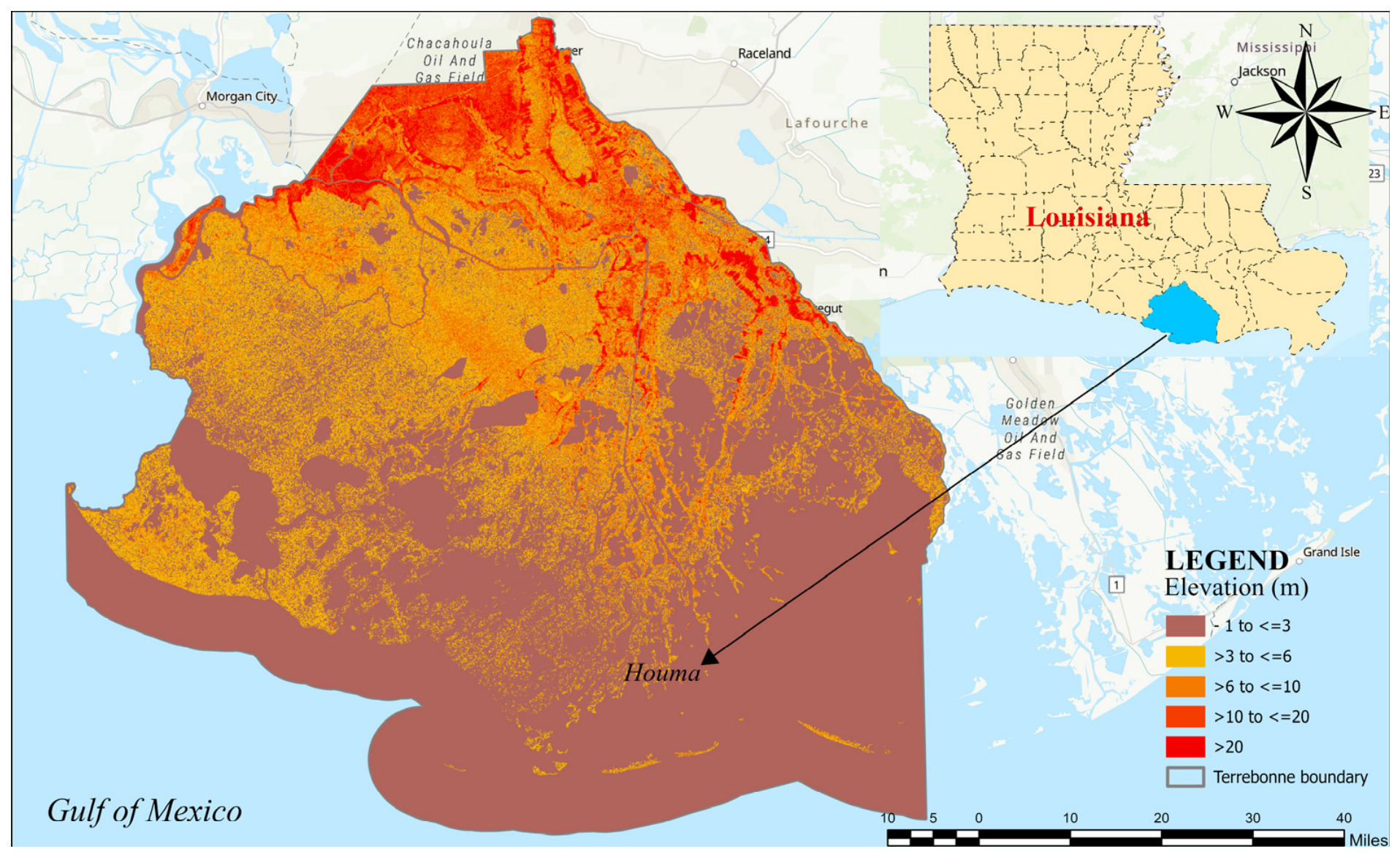
Figure 2.
Overview of the methodological workflow illustrating five principal stages: (1) multi-source conditioning factor compilation; (2) hazard label generation and feature exclusion; (3) training and testing of eight ML/DL algorithms; (4) spatial block cross-validation and SAEML development; and (5) susceptibility map generation and composite index derivation.
Figure 2.
Overview of the methodological workflow illustrating five principal stages: (1) multi-source conditioning factor compilation; (2) hazard label generation and feature exclusion; (3) training and testing of eight ML/DL algorithms; (4) spatial block cross-validation and SAEML development; and (5) susceptibility map generation and composite index derivation.
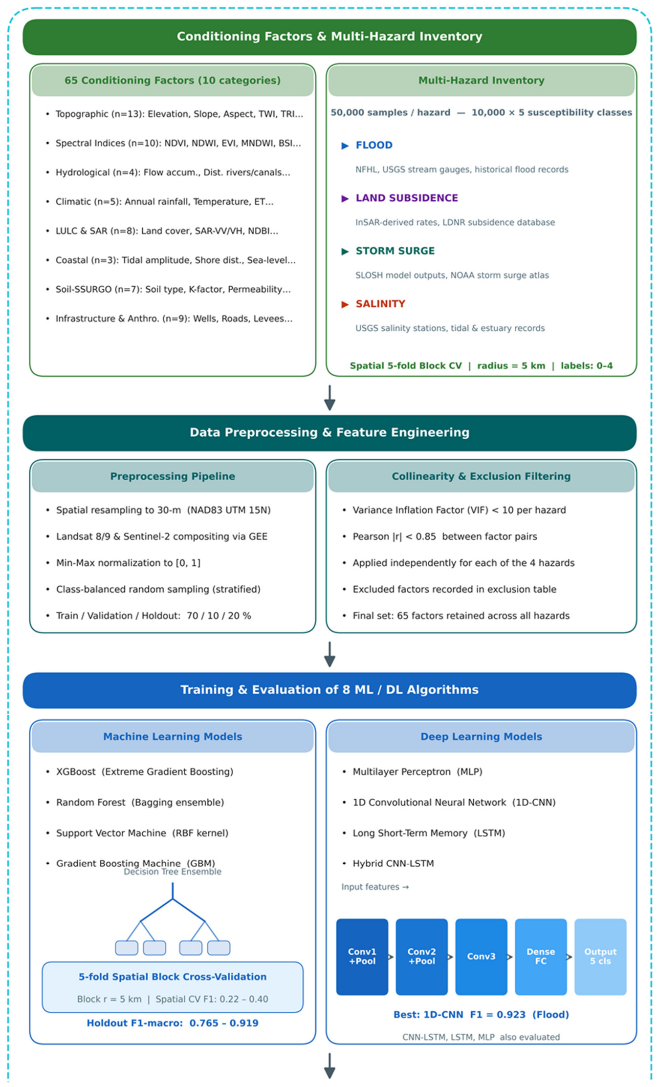
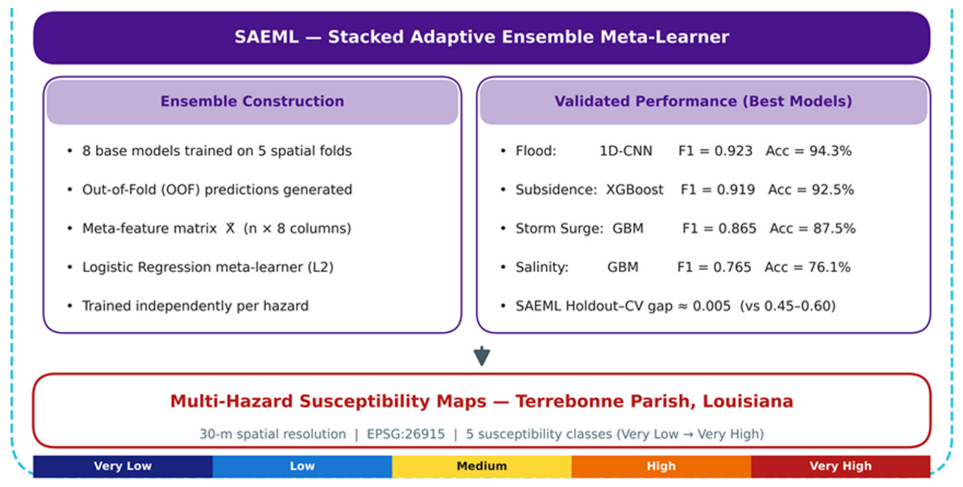
Figure 3.
Holdout F1-macro performance of eight ML and DL algorithms across four co-occurring coastal hazards (Terrebonne Parish). Colored bars represent per-model holdout F1-macro on the independent 15% test set; diamond markers show spatial 5-fold block CV mean ± one standard deviation. The star (★) denotes the best-performing model per hazard based on F1-macro. The large gap between holdout bars and CV diamonds (~53 percentage points on average) quantifies the spatial autocorrelation inflation in conventional holdout evaluation. XGBoost = eXtreme Gradient Boosting; RF = Random Forest; SVM = Support Vector Machine; GBM = Gradient Boosting Machine; MLP = Multilayer Perceptron; 1D-CNN = one-dimensional Convolutional Neural Network; LSTM = Long Short-Term Memory; CNN-LSTM = hybrid CNN-LSTM.
Figure 3.
Holdout F1-macro performance of eight ML and DL algorithms across four co-occurring coastal hazards (Terrebonne Parish). Colored bars represent per-model holdout F1-macro on the independent 15% test set; diamond markers show spatial 5-fold block CV mean ± one standard deviation. The star (★) denotes the best-performing model per hazard based on F1-macro. The large gap between holdout bars and CV diamonds (~53 percentage points on average) quantifies the spatial autocorrelation inflation in conventional holdout evaluation. XGBoost = eXtreme Gradient Boosting; RF = Random Forest; SVM = Support Vector Machine; GBM = Gradient Boosting Machine; MLP = Multilayer Perceptron; 1D-CNN = one-dimensional Convolutional Neural Network; LSTM = Long Short-Term Memory; CNN-LSTM = hybrid CNN-LSTM.
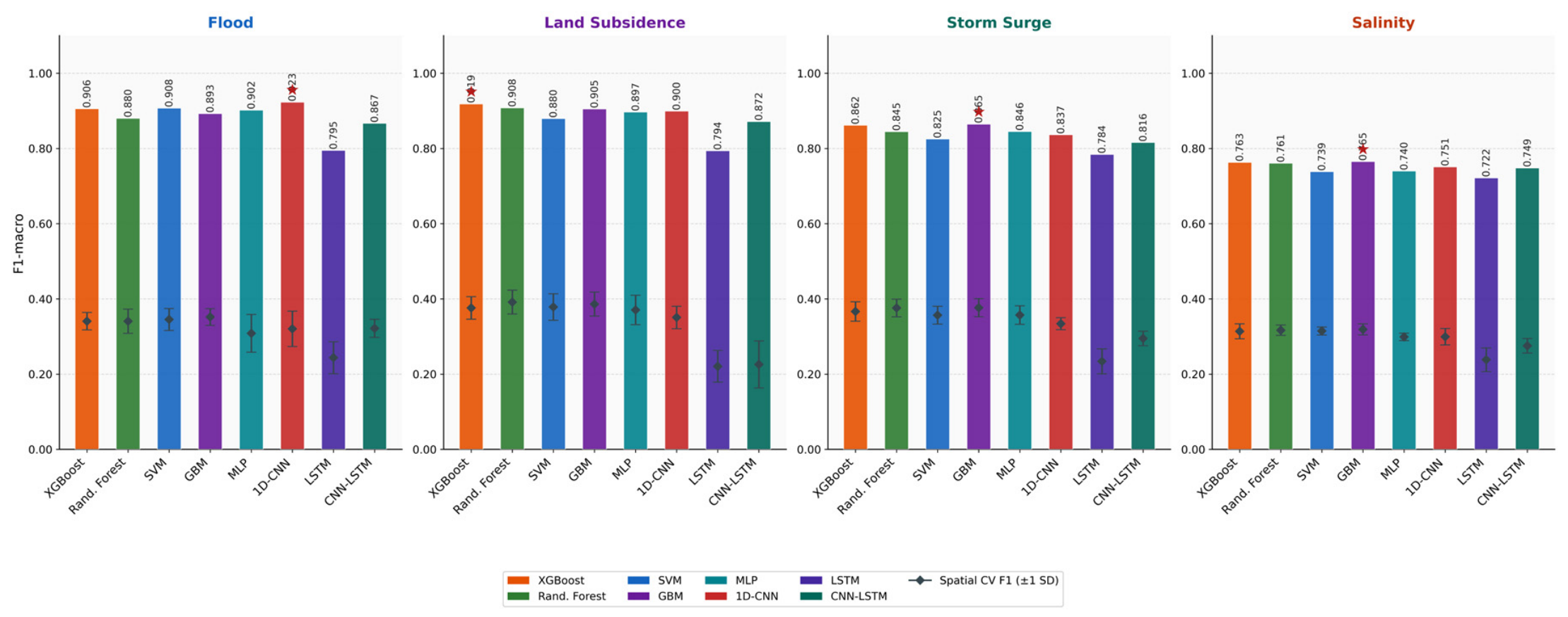
Figure 4.
Model performance radar charts comparing all eight ML and DL algorithms across five evaluation metrics Accuracy, F1-macro, Precision (macro), Recall (macro), and Cohen’s Kappa on the holdout test set for each of the four hazards. All metrics are plotted on their native [0, 1] scale with the y-axis constrained to [0.60, 1.00] to enhance visual differentiation among high-performing models. The 1D-CNN polygon (bold red line) is largest for Flood, confirming its superiority; LSTM consistently displays the smallest polygon, indicating uniformly lowest performance across all metrics and hazards.
Figure 4.
Model performance radar charts comparing all eight ML and DL algorithms across five evaluation metrics Accuracy, F1-macro, Precision (macro), Recall (macro), and Cohen’s Kappa on the holdout test set for each of the four hazards. All metrics are plotted on their native [0, 1] scale with the y-axis constrained to [0.60, 1.00] to enhance visual differentiation among high-performing models. The 1D-CNN polygon (bold red line) is largest for Flood, confirming its superiority; LSTM consistently displays the smallest polygon, indicating uniformly lowest performance across all metrics and hazards.
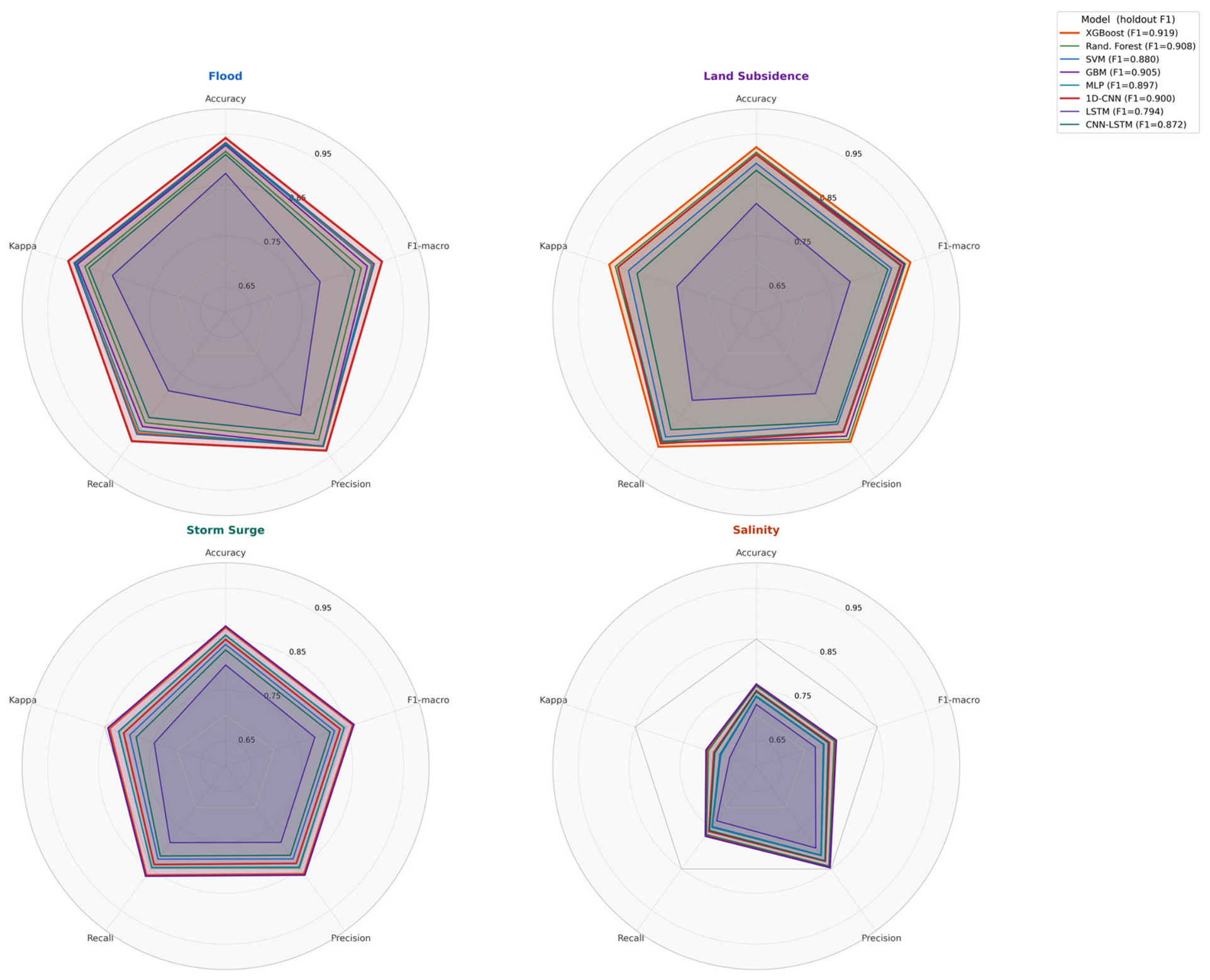
Figure 5.
Normalized confusion matrices for the best-performing model per hazard on the holdout test set. Each cell reports the row-normalized proportion (proportion of true-class samples predicted to each class) with the raw sample count in parentheses. Diagonal values represent correctly classified proportions; off-diagonal values indicate systematic misclassification patterns. Models: Flood = 1D-CNN; Land Subsidence = XGBoost; Storm Surge = GBM; Salinity = GBM. Five susceptibility classes: Very Low (0), Low (1), Moderate (2), High (3), Very High (4).
Figure 5.
Normalized confusion matrices for the best-performing model per hazard on the holdout test set. Each cell reports the row-normalized proportion (proportion of true-class samples predicted to each class) with the raw sample count in parentheses. Diagonal values represent correctly classified proportions; off-diagonal values indicate systematic misclassification patterns. Models: Flood = 1D-CNN; Land Subsidence = XGBoost; Storm Surge = GBM; Salinity = GBM. Five susceptibility classes: Very Low (0), Low (1), Moderate (2), High (3), Very High (4).
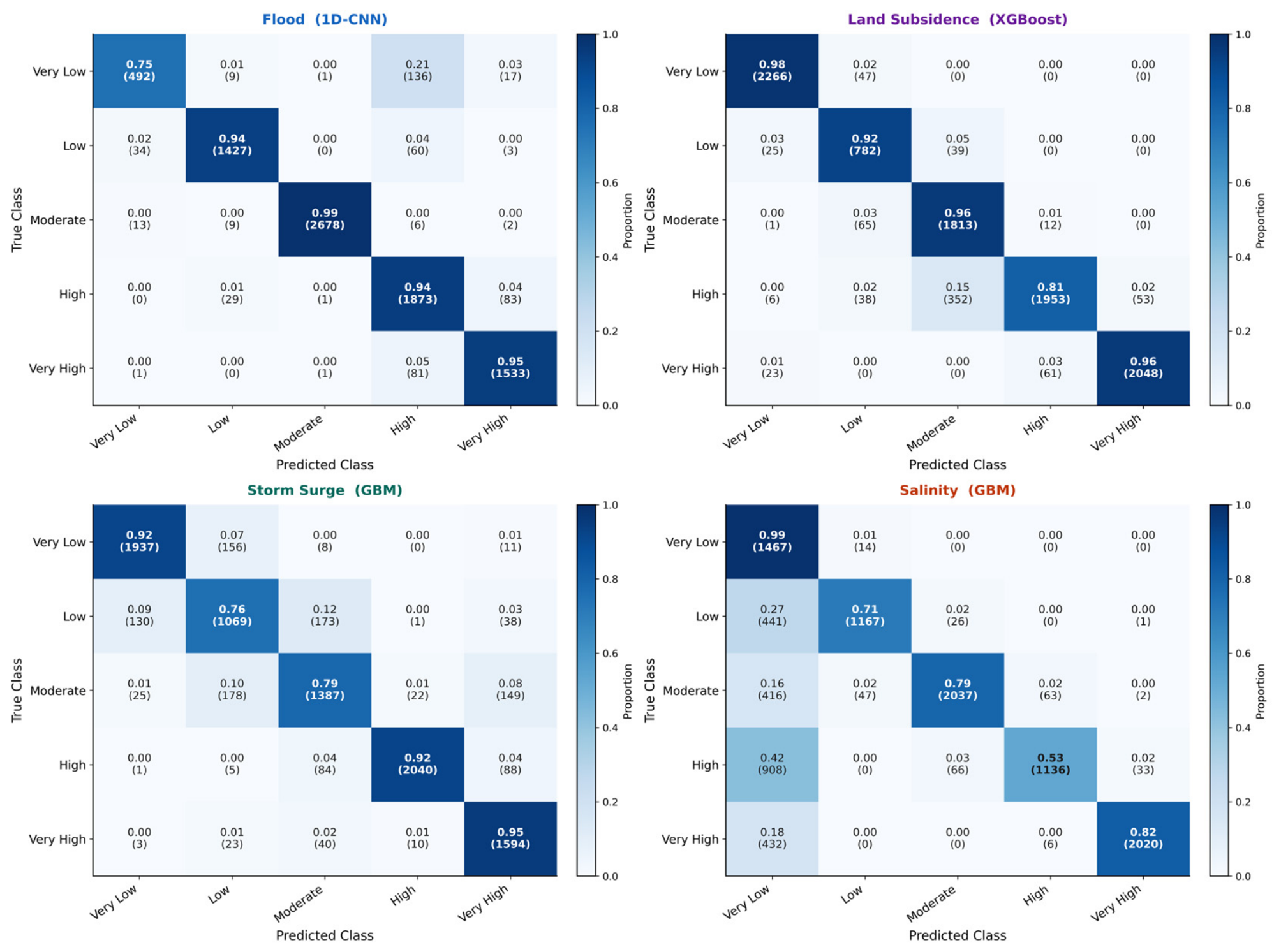
Figure 6.
Macro-average one-vs-rest (OvR) ROC curves for all eight ML and DL models evaluated on the holdout test set across four hazards. Each curve represents the mean ROC computed across five binary OvR classifiers (one per susceptibility class) with the corresponding macro-average AUC in the legend. The bold line highlights the best-performing model per hazard (1D-CNN for flood; XGBoost for subsidence; GBM for storm surge and salinity). AUC values represent upper bounds on discriminative capacity under holdout evaluation; expected AUC under spatial cross-validation would be substantially lower.
Figure 6.
Macro-average one-vs-rest (OvR) ROC curves for all eight ML and DL models evaluated on the holdout test set across four hazards. Each curve represents the mean ROC computed across five binary OvR classifiers (one per susceptibility class) with the corresponding macro-average AUC in the legend. The bold line highlights the best-performing model per hazard (1D-CNN for flood; XGBoost for subsidence; GBM for storm surge and salinity). AUC values represent upper bounds on discriminative capacity under holdout evaluation; expected AUC under spatial cross-validation would be substantially lower.
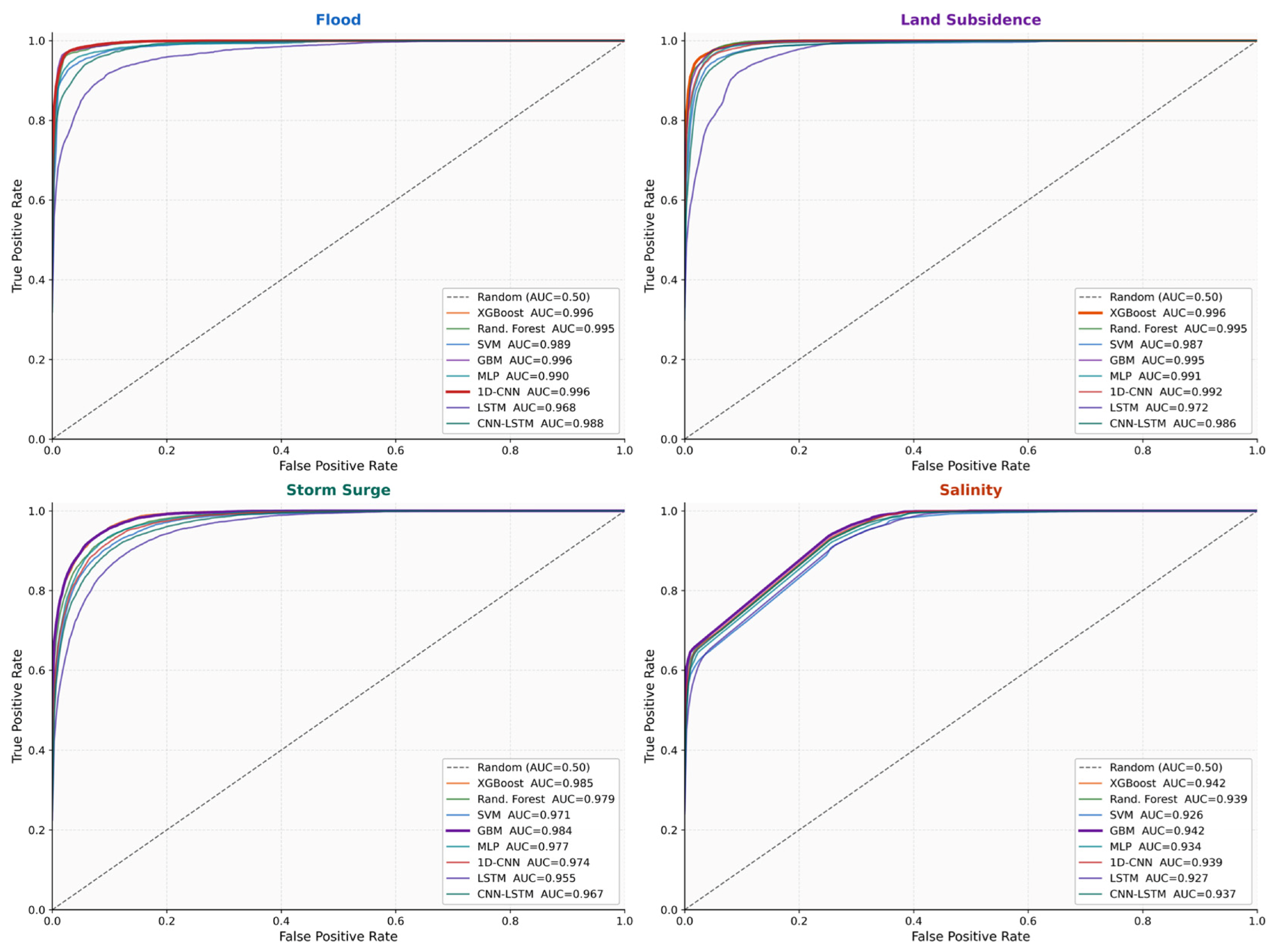
Figure 7.
Top 10 conditioning factors per hazard ranked by mean permutation importance aggregated across XGBoost, Random Forest, and GBM on the holdout test set. Importance scores represent the mean F1 macro decrease upon random permutation of each predictor, averaged over five permutation repetitions per factor. Longer bars indicate greater model reliance on that factor. The best-performing model per hazard is annotated in each panel. Factors are color-coded by hazard: blue = Flood; purple = Land Subsidence; teal = Storm Surge; red = Salinity.
Figure 7.
Top 10 conditioning factors per hazard ranked by mean permutation importance aggregated across XGBoost, Random Forest, and GBM on the holdout test set. Importance scores represent the mean F1 macro decrease upon random permutation of each predictor, averaged over five permutation repetitions per factor. Longer bars indicate greater model reliance on that factor. The best-performing model per hazard is annotated in each panel. Factors are color-coded by hazard: blue = Flood; purple = Land Subsidence; teal = Storm Surge; red = Salinity.
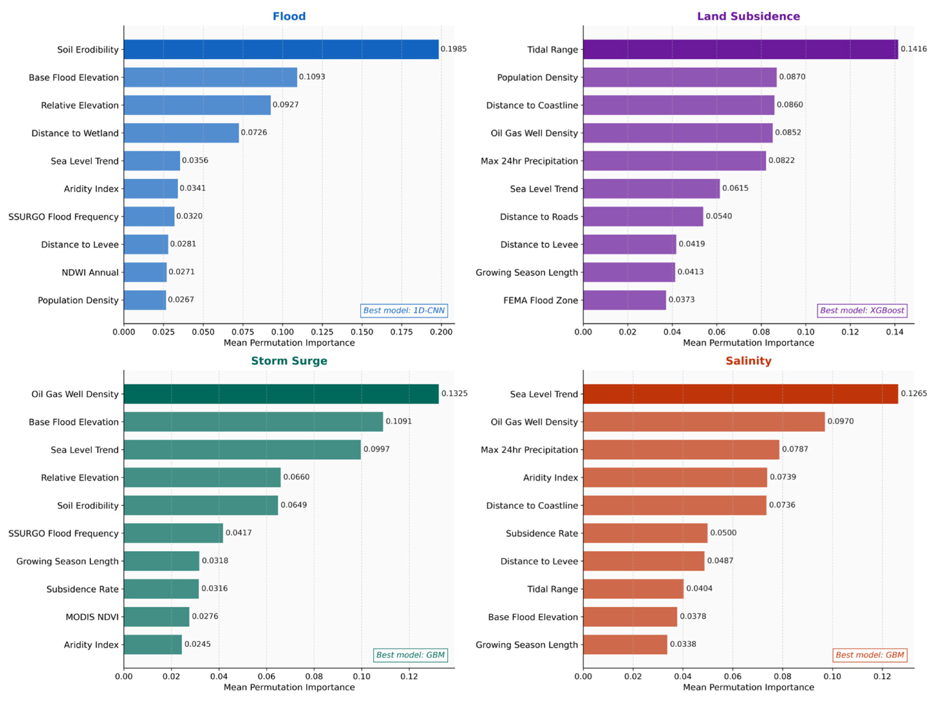
Figure 8.
Feature importance radar charts comparing three tree-based algorithms XGBoost (orange), Random Forest (green), and GBM (purple) across the top 10 conditioning factors per hazard. Importance scores are normalized to [0, 1] per model so that polygon shapes reflect the relative factor hierarchy rather than absolute magnitude. Larger polygons indicate more distributed factor reliance; concentrated polygons indicate dominance by one or two predictors. The contrasting polygon geometries between XGBoost (peaked) and GBM/RF (flatter) illustrate their differing feature weighting strategies, with GBM’s broader distribution consistent with its superior spatial cross-validation performance.
Figure 8.
Feature importance radar charts comparing three tree-based algorithms XGBoost (orange), Random Forest (green), and GBM (purple) across the top 10 conditioning factors per hazard. Importance scores are normalized to [0, 1] per model so that polygon shapes reflect the relative factor hierarchy rather than absolute magnitude. Larger polygons indicate more distributed factor reliance; concentrated polygons indicate dominance by one or two predictors. The contrasting polygon geometries between XGBoost (peaked) and GBM/RF (flatter) illustrate their differing feature weighting strategies, with GBM’s broader distribution consistent with its superior spatial cross-validation performance.
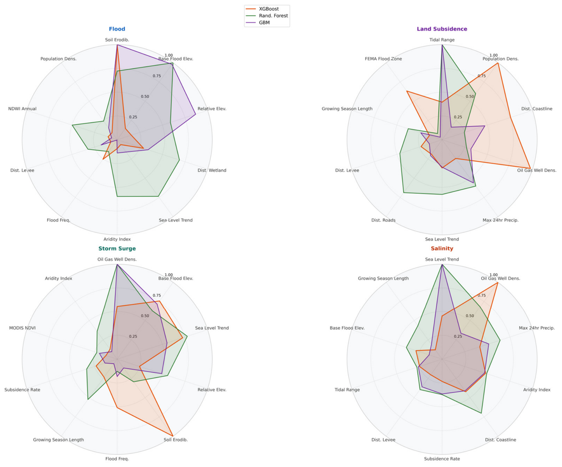
Figure 9.
Five-class susceptibility maps at 30-m resolution for Terrebonne Parish: (a) flood (1D-CNN); (b) land subsidence (XGBoost); (c) storm surge (GBM); (d) salinity intrusion (GBM). Classes: Very Low (0) to Very High (4).
Figure 9.
Five-class susceptibility maps at 30-m resolution for Terrebonne Parish: (a) flood (1D-CNN); (b) land subsidence (XGBoost); (c) storm surge (GBM); (d) salinity intrusion (GBM). Classes: Very Low (0) to Very High (4).
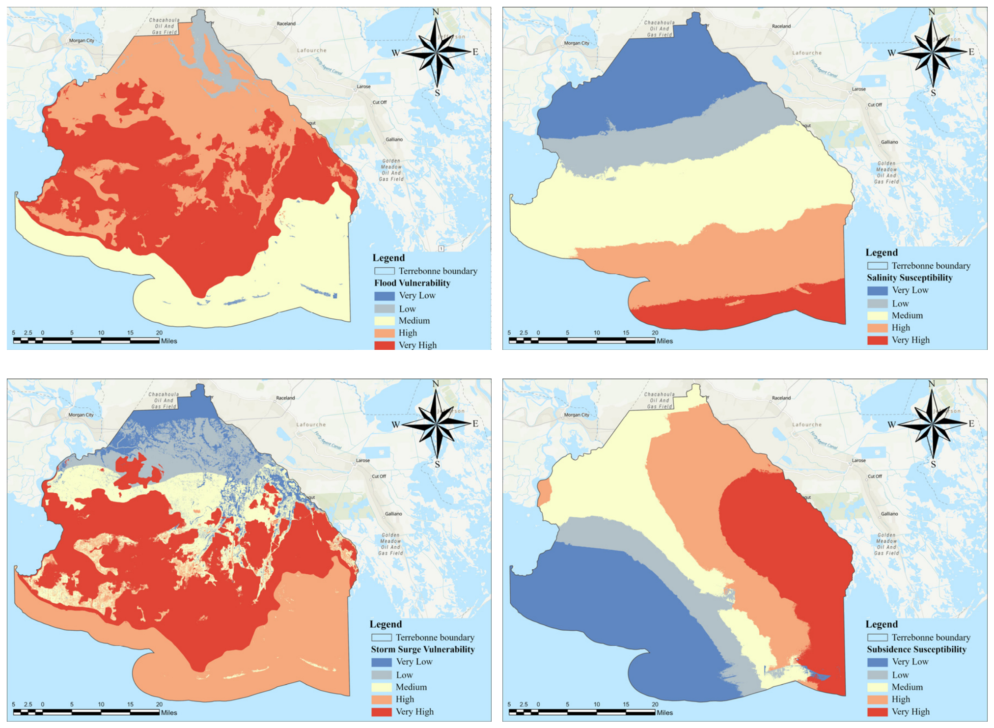
Figure 10.
Composite multi-hazard susceptibility index (MHSI) for Terrebonne Parish, computed as the arithmetic mean of normalized class values across the four hazard maps. Range: 0.125–0.938; Mean = 0.574; Std = 0.135.
Figure 10.
Composite multi-hazard susceptibility index (MHSI) for Terrebonne Parish, computed as the arithmetic mean of normalized class values across the four hazard maps. Range: 0.125–0.938; Mean = 0.574; Std = 0.135.
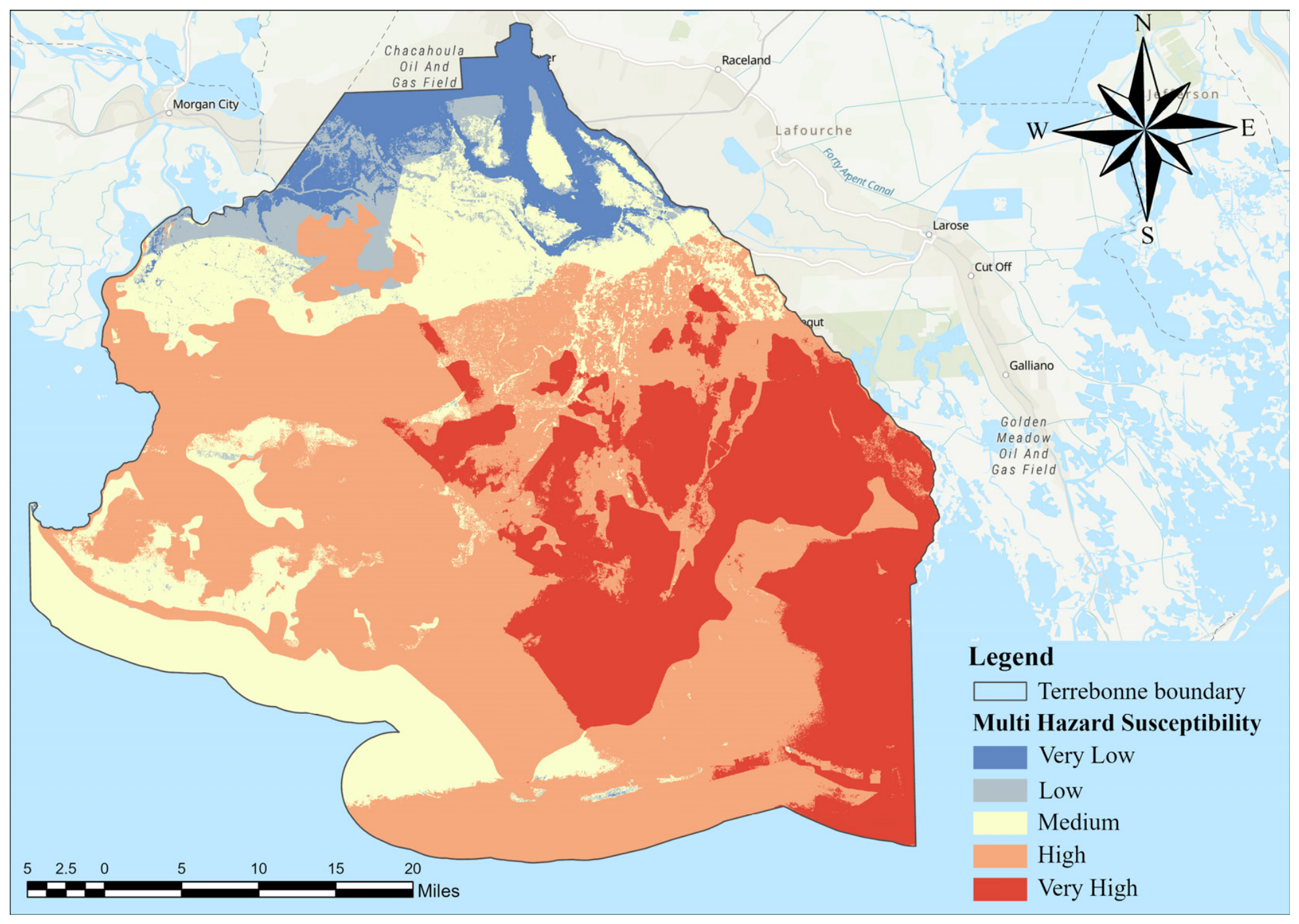

Table 1.
The 65 environmental conditioning factors compiled for multi-hazard susceptibility mapping in Terrebonne Parish, organized by thematic category. GEE = Google Earth Engine; NHD = National Hydrography Dataset; NLCD = National Land Cover Database; SSURGO = Soil Survey Geographic Database; LA = Louisiana; Res. = spatial resolution.
Table 1.
The 65 environmental conditioning factors compiled for multi-hazard susceptibility mapping in Terrebonne Parish, organized by thematic category. GEE = Google Earth Engine; NHD = National Hydrography Dataset; NLCD = National Land Cover Database; SSURGO = Soil Survey Geographic Database; LA = Louisiana; Res. = spatial resolution.
| No. | Factor | Category | Source | Res. |
|---|---|---|---|---|
| 1 | Aspect | Topographic | 30-m DEM derivative | 30 m |
| 2 | Convergence Index | Topographic | 30-m DEM derivative | 30 m |
| 3 | Elevation | Topographic | USGS 3DEP/SRTM | 30 m |
| 4 | Hill shade | Topographic | 30-m DEM derivative | 30 m |
| 5 | Plan Curvature | Topographic | 30-m DEM derivative | 30 m |
| 6 | Profile Curvature | Topographic | 30-m DEM derivative | 30 m |
| 7 | Slope | Topographic | 30-m DEM derivative | 30 m |
| 8 | SPI | Topographic | 30-m DEM derivative | 30 m |
| 9 | Total Curvature | Topographic | 30-m DEM derivative | 30 m |
| 10 | TPI-Large | Topographic | 30-m DEM derivative | 30 m |
| 11 | TPI-Small | Topographic | 30-m DEM derivative | 30 m |
| 12 | TRI | Topographic | 30-m DEM derivative | 30 m |
| 13 | TWI | Topographic | 30-m DEM derivative | 30 m |
| 14 | BSI | Spectral | Sentinel-2/Landsat (GEE) | 30 m |
| 15 | EVI | Spectral | Sentinel-2/Landsat (GEE) | 30 m |
| 16 | MNDWI | Spectral | Sentinel-2/Landsat (GEE) | 30 m |
| 17 | NDBI | Spectral | Sentinel-2/Landsat (GEE) | 30 m |
| 18 | NDSI | Spectral | Sentinel-2/Landsat (GEE) | 30 m |
| 19 | NDVI | Spectral | Sentinel-2/Landsat (GEE) | 30 m |
| 20 | NDWI | Spectral | Sentinel-2/Landsat (GEE) | 30 m |
| 21 | SAVI | Spectral | Sentinel-2/Landsat (GEE) | 30 m |
| 22 | SI-1 | Spectral | Sentinel-2/Landsat (GEE) | 30 m |
| 23 | SI-3 | Spectral | Sentinel-2/Landsat (GEE) | 30 m |
| 24 | Dist. to Coastline | Hydrological | NHD/coastline shapefile | 30 m |
| 25 | Dist. to Rivers | Hydrological | NHD flowlines | 30 m |
| 26 | Dist. to Waterbodies | Hydrological | NHD waterbodies | 30 m |
| 27 | Drainage Density | Hydrological | NHD flowlines (derived) | 30 m |
| 28 | Aridity Index | Climate | PRISM/WorldClim v2 | 30 m |
| 29 | Growing Season Length | Climate | PRISM/NOAA | 30 m |
| 30 | Max 24-h Precip. | Climate | PRISM | 30 m |
| 31 | Mean Annual Precip. | Climate | PRISM | 30 m |
| 32 | Precip. Seasonality | Climate | WorldClim v2 | 30 m |
| 33 | Dist. to Roads | Anthropogenic | TIGER/Line Roads | 30 m |
| 34 | Population Density | Anthropogenic | LandScan/Census 2020 | 30 m |
| 35 | Road Density | Anthropogenic | TIGER/Line Roads (derived) | 30 m |
| 36 | Mean High Water | Coastal | NOAA CO-OPS tidal gauges | 30 m |
| 37 | Sea Level Trend | Coastal | NOAA CO-OPS tidal gauges | 30 m |
| 38 | Tidal Range | Coastal | NOAA CO-OPS tidal gauges | 30 m |
| 39 | Dist. to Urban | LULC | NLCD 2021 | 30 m |
| 40 | Dist. to Wetland | LULC | NLCD 2021 | 30 m |
| 41 | Evapotranspiration | LULC | MODIS MOD16A2 | 500 m->30 m |
| 42 | Land Surface Temp. | LULC | MODIS MOD11A1 | 1 km->30 m |
| 43 | LULC Type | LULC | NLCD 2021 | 30 m |
| 44 | SAR VH | LULC | Sentinel-1 GRD (GEE) | 10 m->30 m |
| 45 | SAR VV | LULC | Sentinel-1 GRD (GEE) | 10 m->30 m |
| 46 | Water Occurrence | LULC | JRC Global Surface Water | 30 m |
| 47 | Base Flood Elevation | Hazard Infra. | FEMA FIRM/BFE grid | 30 m |
| 48 | Canal Density | Hazard Infra. | LA hydrography layer | 30 m |
| 49 | Dist. to Levee | Hazard Infra. | USACE/CPRA levee data | 30 m |
| 50 | FEMA Flood Zone | Hazard Infra. | FEMA FIRM (2023) | 30 m |
| 51 | Oil/Gas Well Density | Hazard Infra. | Louisiana DNR well registry | 30 m |
| 52 | Bulk Density | Geophysical | POLARIS soil dataset | 30 m |
| 53 | MODIS NDVI | Geophysical | MODIS MOD13A3 | 1 km->30 m |
| 54 | NDVI Seasonal Var. | Geophysical | MODIS MOD13A3 (derived) | 30 m |
| 55 | NDWI Seasonal Var. | Geophysical | Sentinel-2/Landsat (GEE) | 30 m |
| 56 | Relative Elevation | Geophysical | DEM/NHD (derived) | 30 m |
| 57 | Soil Erodibility (K) | Geophysical | USDA SSURGO | 30 m |
| 58 | Subsidence Rate | Geophysical | InSAR/GPS geodetic data | 30 m |
| 59 | SSURGO Drain. Class | Soil | USDA SSURGO (2023) | 30 m |
| 60 | SSURGO Flood Freq. | Soil | USDA SSURGO (2023) | 30 m |
| 61 | SSURGO Hydro. Group | Soil | USDA SSURGO (2023) | 30 m |
| 62 | SSURGO Ksat | Soil | USDA SSURGO (2023) | 30 m |
| 63 | SSURGO Organic Matter | Soil | USDA SSURGO (2023) | 30 m |
| 64 | SSURGO Pond Freq. | Soil | USDA SSURGO (2023) | 30 m |
| 65 | SSURGO Water Table | Soil | USDA SSURGO (2023) | 30 m |
Table 2.
Feature exclusion per hazard to prevent circular reasoning in susceptibility modeling.
| Hazard | Total | Included | Excluded (n) | Excluded Features |
|---|---|---|---|---|
| Flood | 65 | 60 | 5 | Elevation, TWI, Dist. to Rivers, Dist. to Waterbodies, FEMA Flood Zone |
| Subsidence | 65 | 64 | 1 | Subsidence Rate |
| Storm Surge | 65 | 62 | 3 | Elevation, Dist. to Coastline, FEMA Flood Zone |
| Salinity | 65 | 65 | 0 | None (labels from USGS water quality monitoring) |
Table 3.
Complete holdout test performance for all 32 base models (Terrebonne Parish). * = best model per hazard based on F1-macro. n = conditioning factors after exclusion; Acc. = Overall Accuracy; F1-wt = F1-weighted.
Table 3.
Complete holdout test performance for all 32 base models (Terrebonne Parish). * = best model per hazard based on F1-macro. n = conditioning factors after exclusion; Acc. = Overall Accuracy; F1-wt = F1-weighted.
| Hazard | Model | n | Acc. | F1-Macro | F1-wt | Kappa | Time (s) |
|---|---|---|---|---|---|---|---|
| Flood | XGBoost | 60 | 0.9337 | 0.9058 | 0.9323 | 0.9134 | 5.2 |
| Flood | Random Forest | 60 | 0.9164 | 0.8804 | 0.9159 | 0.8910 | 2.0 |
| Flood | SVM | 60 | 0.9330 | 0.9076 | 0.9320 | 0.9126 | 14.8 |
| Flood | GBM | 60 | 0.9283 | 0.8930 | 0.9259 | 0.9062 | 196.1 |
| Flood | MLP | 60 | 0.9309 | 0.9022 | 0.9293 | 0.9097 | 9.7 |
| Flood | 1D-CNN * | 60 | 0.9427 | 0.9232 | 0.9424 | 0.9254 | 72.4 |
| Flood | LSTM | 60 | 0.8730 | 0.7952 | 0.8646 | 0.8340 | 471.4 |
| Flood | CNN-LSTM | 60 | 0.9101 | 0.8671 | 0.9075 | 0.8827 | 156.5 |
| Subsidence | XGBoost * | 64 | 0.9247 | 0.9186 | 0.9247 | 0.9041 | 2.9 |
| Subsidence | Random Forest | 64 | 0.9145 | 0.9083 | 0.9146 | 0.8913 | 1.2 |
| Subsidence | SVM | 64 | 0.8928 | 0.8796 | 0.8936 | 0.8644 | 20.2 |
| Subsidence | GBM | 64 | 0.9107 | 0.9053 | 0.9102 | 0.8865 | 238.5 |
| Subsidence | MLP | 64 | 0.9100 | 0.8972 | 0.9105 | 0.8857 | 11.1 |
| Subsidence | 1D-CNN | 64 | 0.9100 | 0.8996 | 0.9099 | 0.8858 | 115.7 |
| Subsidence | LSTM | 64 | 0.8138 | 0.7942 | 0.8132 | 0.7642 | 555.2 |
| Subsidence | CNN-LSTM | 64 | 0.8791 | 0.8720 | 0.8774 | 0.8464 | 199.6 |
| Storm Surge | XGBoost | 62 | 0.8720 | 0.8620 | 0.8728 | 0.8392 | 4.1 |
| Storm Surge | Random Forest | 62 | 0.8572 | 0.8450 | 0.8574 | 0.8206 | 1.3 |
| Storm Surge | SVM | 62 | 0.8395 | 0.8254 | 0.8402 | 0.7983 | 48.4 |
| Storm Surge | GBM * | 62 | 0.8752 | 0.8650 | 0.8754 | 0.8432 | 256.8 |
| Storm Surge | MLP | 62 | 0.8582 | 0.8455 | 0.8583 | 0.8216 | 7.5 |
| Storm Surge | 1D-CNN | 62 | 0.8493 | 0.8368 | 0.8505 | 0.8108 | 108.3 |
| Storm Surge | LSTM | 62 | 0.7990 | 0.7845 | 0.8012 | 0.7476 | 566.5 |
| Storm Surge | CNN-LSTM | 62 | 0.8286 | 0.8162 | 0.8310 | 0.7850 | 215.1 |
| Salinity | XGBoost | 65 | 0.7592 | 0.7633 | 0.7818 | 0.7012 | 2.4 |
| Salinity | Random Forest | 65 | 0.7576 | 0.7610 | 0.7793 | 0.6991 | 1.0 |
| Salinity | SVM | 65 | 0.7364 | 0.7386 | 0.7568 | 0.6732 | 95.0 |
| Salinity | GBM * | 65 | 0.7612 | 0.7654 | 0.7837 | 0.7037 | 172.6 |
| Salinity | MLP | 65 | 0.7382 | 0.7402 | 0.7580 | 0.6754 | 9.6 |
| Salinity | 1D-CNN | 65 | 0.7482 | 0.7512 | 0.7691 | 0.6877 | 89.8 |
| Salinity | LSTM | 65 | 0.7215 | 0.7221 | 0.7404 | 0.6549 | 516.1 |
| Salinity | CNN-LSTM | 65 | 0.7465 | 0.7485 | 0.7662 | 0.6854 | 197.8 |
Table 4.
Per-class F1 scores for the best-performing model per hazard (Terrebonne Parish).
| Hazard | Best Model | F1 (V. Low) | F1 (Low) | F1 (Mod.) | F1 (High) | F1 (V. High) |
|---|---|---|---|---|---|---|
| Flood | 1D-CNN | 0.8234 | 0.9520 | 0.9939 | 0.9044 | 0.9422 |
| Subsidence | XGBoost | 0.9780 | 0.8796 | 0.8855 | 0.8821 | 0.9676 |
| Storm Surge | GBM | 0.9206 | 0.7523 | 0.8034 | 0.9508 | 0.8980 |
| Salinity | GBM | 0.5703 | 0.8152 | 0.8679 | 0.6786 | 0.8950 |
Table 5.
Spatial cross-validation results (mean +/− std across 5 folds) for all 32 base models (Terrebonne Parish). F1 = F1-macro; Acc. = Overall Accuracy.
Table 5.
Spatial cross-validation results (mean +/− std across 5 folds) for all 32 base models (Terrebonne Parish). F1 = F1-macro; Acc. = Overall Accuracy.
| Hazard | Model | CV F1 Mean | CV F1 Std | CV Acc. Mean | CV Kappa Mean |
|---|---|---|---|---|---|
| Flood | XGBoost | 0.3407 | 0.0232 | 0.3665 | 0.1947 |
| Flood | Random Forest | 0.3407 | 0.0322 | 0.3845 | 0.2127 |
| Flood | SVM | 0.3453 | 0.0291 | 0.3770 | 0.2061 |
| Flood | GBM | 0.3519 | 0.0224 | 0.3706 | 0.2020 |
| Flood | MLP | 0.3086 | 0.0502 | 0.3916 | 0.2155 |
| Flood | 1D-CNN | 0.3204 | 0.0470 | 0.3960 | 0.2198 |
| Flood | LSTM | 0.2437 | 0.0424 | 0.3397 | 0.1459 |
| Flood | CNN-LSTM | 0.3219 | 0.0240 | 0.3886 | 0.2182 |
| Subsidence | XGBoost | 0.3760 | 0.0300 | 0.4019 | 0.2465 |
| Subsidence | Random Forest | 0.3916 | 0.0318 | 0.4151 | 0.2615 |
| Subsidence | SVM | 0.3785 | 0.0352 | 0.4043 | 0.2490 |
| Subsidence | GBM | 0.3862 | 0.0317 | 0.4025 | 0.2463 |
| Subsidence | MLP | 0.3707 | 0.0391 | 0.4133 | 0.2605 |
| Subsidence | 1D-CNN | 0.3507 | 0.0299 | 0.3859 | 0.2247 |
| Subsidence | LSTM | 0.2208 | 0.0421 | 0.2935 | 0.1138 |
| Subsidence | CNN-LSTM | 0.2258 | 0.0624 | 0.2829 | 0.1075 |
| Storm Surge | XGBoost | 0.3665 | 0.0258 | 0.3886 | 0.2278 |
| Storm Surge | Random Forest | 0.3759 | 0.0235 | 0.3965 | 0.2379 |
| Storm Surge | SVM | 0.3568 | 0.0236 | 0.3675 | 0.2042 |
| Storm Surge | GBM | 0.3767 | 0.0239 | 0.3893 | 0.2295 |
| Storm Surge | MLP | 0.3571 | 0.0245 | 0.3835 | 0.2238 |
| Storm Surge | 1D-CNN | 0.3342 | 0.0159 | 0.3652 | 0.1995 |
| Storm Surge | LSTM | 0.2340 | 0.0332 | 0.3053 | 0.1333 |
| Storm Surge | CNN-LSTM | 0.2950 | 0.0193 | 0.3385 | 0.1686 |
| Salinity | XGBoost | 0.3139 | 0.0198 | 0.3416 | 0.1754 |
| Salinity | Random Forest | 0.3168 | 0.0137 | 0.3640 | 0.2026 |
| Salinity | SVM | 0.3147 | 0.0106 | 0.3500 | 0.1857 |
| Salinity | GBM | 0.3190 | 0.0146 | 0.3519 | 0.1873 |
| Salinity | MLP | 0.2991 | 0.0098 | 0.3653 | 0.2044 |
| Salinity | 1D-CNN | 0.2994 | 0.0219 | 0.3420 | 0.1755 |
| Salinity | LSTM | 0.2383 | 0.0313 | 0.2941 | 0.1167 |
| Salinity | CNN-LSTM | 0.2753 | 0.0193 | 0.3282 | 0.1570 |
Table 6.
Top 10 conditioning factors per hazard ranked by aggregate permutation importance (mean across XGBoost, RF, GBM) for Terrebonne Parish.
Table 6.
Top 10 conditioning factors per hazard ranked by aggregate permutation importance (mean across XGBoost, RF, GBM) for Terrebonne Parish.
| Rank | Flood | Imp. | Subsidence | Imp. | Storm Surge | Imp. | Salinity | Imp. |
|---|---|---|---|---|---|---|---|---|
| 1 | Soil Erodibility | 0.199 | Tidal Range | 0.142 | Oil Gas Well Dens. | 0.133 | Sea Level Trend | 0.126 |
| 2 | Base Flood Elev. | 0.109 | Population Density | 0.087 | Base Flood Elev. | 0.109 | Oil Gas Well Dens. | 0.097 |
| 3 | Relative Elev. | 0.093 | Dist. to Coastline | 0.086 | Sea Level Trend | 0.100 | Max 24hr Precip. | 0.079 |
| 4 | Dist. to Wetland | 0.073 | Oil Gas Well Dens. | 0.085 | Relative Elevation | 0.066 | Aridity Index | 0.074 |
| 5 | Sea Level Trend | 0.036 | Max 24hr Precip. | 0.082 | Soil Erodibility | 0.065 | Dist. to Coastline | 0.074 |
| 6 | Aridity Index | 0.034 | Sea Level Trend | 0.061 | SSURGO Flood Freq. | 0.042 | Subsidence Rate | 0.050 |
| 7 | SSURGO Flood Freq. | 0.032 | Dist. to Roads | 0.054 | Growing Season | 0.032 | Dist. to Levee | 0.049 |
| 8 | Dist. to Levee | 0.028 | Dist. to Levee | 0.042 | Subsidence Rate | 0.032 | Tidal Range | 0.040 |
| 9 | NDWI Annual | 0.027 | Growing Season | 0.041 | MODIS NDVI | 0.028 | Base Flood Elev. | 0.038 |
| 10 | Population Density | 0.027 | FEMA Flood Zone | 0.037 | Aridity Index | 0.024 | Growing Season | 0.034 |
Table 7.
SAEML performance versus best base model per hazard (Terrebonne Parish). Gap = Holdout F1—Spatial CV F1 (near-zero gap indicates spatial honesty). CV F1 = mean F1-macro across 5 spatial CV folds.
Table 7.
SAEML performance versus best base model per hazard (Terrebonne Parish). Gap = Holdout F1—Spatial CV F1 (near-zero gap indicates spatial honesty). CV F1 = mean F1-macro across 5 spatial CV folds.
| Hazard | Best Base Model | Base Holdout F1 | Base CV F1 | SAEML Holdout F1 | SAEML CV F1 | SAEML Gap | Base Gap |
|---|---|---|---|---|---|---|---|
| Flood | 1D-CNN | 0.9232 | 0.3204 | 0.3355 | 0.3404 | ~0.005 | ~0.603 |
| Subsidence | XGBoost | 0.9186 | 0.3760 | 0.3685 | 0.3641 | ~0.004 | ~0.543 |
| Storm Surge | GBM | 0.8650 | 0.3767 | 0.3563 | 0.3536 | ~0.003 | ~0.488 |
| Salinity | GBM | 0.7654 | 0.3190 | 0.3037 | 0.3096 | ~-0.006 | ~0.446 |
Disclaimer/Publisher’s Note: The statements, opinions and data contained in all publications are solely those of the individual author(s) and contributor(s) and not of MDPI and/or the editor(s). MDPI and/or the editor(s) disclaim responsibility for any injury to people or property resulting from any ideas, methods, instructions or products referred to in the content. |
© 2026 by the authors. Licensee MDPI, Basel, Switzerland. This article is an open access article distributed under the terms and conditions of the Creative Commons Attribution (CC BY) license (http://creativecommons.org/licenses/by/4.0/).
Copyright: This open access article is published under a Creative Commons CC BY 4.0 license, which permit the free download, distribution, and reuse, provided that the author and preprint are cited in any reuse.