

Submitted:
24 June 2026
Posted:
25 June 2026
You are already at the latest version
Abstract
Traditional attribute control charts for defect counts are commonly developed under the assumption that count data follow a homogeneous Poisson distribution. However, this assumption is often violated in practical applications. To overcome this limitation, a two-parameter Poisson distribution, the Conway-Maxwell-Poisson (CMP or COM-Poisson) distribution, has been widely used to construct control charts capable of effectively monitoring count data exhibiting over- or under-dispersion. Furthermore, the multiple dependent state (MDS) sampling scheme evaluates the current process status not only based on the present sample but also by incorporating information from previous samples, thereby achieving higher detection efficiency than single sampling schemes. This study integrates the COM-Poisson distribution with the MDS sampling strategy to develop an attribute control chart based on the extended exponentially weighted moving average statistic. The average run length is obtained under various shift magnitudes using probability-based computations. The simulation results demonstrate that the proposed chart substantially outperforms existing approaches in the prompt detection of out-of-control conditions. A real-world air quality index (AQI) monitoring study showed that the proposed chart effectively detected increases in weekly AQI counts and provided earlier warnings of potential air quality deterioration.
Keywords:
average run length
; count data
; COM-Poisson distribution
; extended EWMA control chart
; multiple dependent state sampling
1. Introduction
Control charts are the core tools of statistical process control. They are designed to monitor process conditions in real time through statistical methods, reduce variability in quality characteristics, and thus improve process stability. According to the quality characteristic type, Shewhart classified control charts into two major categories: variable and attribute charts. Variable charts deal with continuous data, such as length, weight, and time, with typical examples including and charts. Attribute charts handle categorical or count data, such as the number of conforming and nonconforming items. Common charts of this type include the p, np, c, and u charts, which are based on binomial or Poisson distributions. However, conventional Shewhart charts rely primarily on a single sample at each sampling epoch, which limits their sensitivity to small and moderate process shifts and does not fully exploit historical information. Roberts [1] proposed the exponentially weighted moving average (EWMA) chart, which combines current and past observations through a recursive weighting scheme to enhance the detection of small shifts. Its extension, the extended EWMA (EEWMA) chart, can further reduce the average run length (ARL) under out-of-control conditions by appropriately selecting smoothing parameters, thereby improving process monitoring responsiveness and efficiency. Subsequently, Naveed et al. [2] proposed an EEWMA control chart that when appropriate smoothing parameters are chosen, can reduce the out-of-control ARL, thereby enhancing process monitoring responsiveness and efficiency.
Traditional attribute control charts for count data are constructed under the Poisson assumption that the mean is equal to the variance, which is often violated in practice because of over- or under-dispersion. Conway and Maxwell [3] addressed this issue by proposing the two-parameter Conway-Maxwell-Poisson (COM-Poisson) distribution, which can accommodate both over- and under-dispersed data and includes Geometric, Poisson, and Bernoulli distributions as special cases. Building on this framework, Saghir and Lin [4] developed the Generalized EWMA (GEWMA) control chart for monitoring COM-Poisson count data and empirically demonstrated that it yields superior ARL performance compared to the Sellers [5] control chart. Aslam et al. [6] applied a repetitive sampling scheme to the GEWMA control chart for the COM-Poisson distribution and found that the proposed chart can outperform the conventional GEWMA chart by yielding smaller ARL values. Aslam et al. [7] proposed a modified EWMA control chart for processes that follow a COM-Poisson distribution and demonstrated that the proposed chart detects out-of-control conditions more rapidly than existing control charts, as evidenced by improved ARL performance. Alevizakos and Koukouvinos [8] introduced a double EWMA control chart for monitoring COM-Poisson attribute data, referred to as the CMP-DEWMA chart and showed that this chart outperforms the standard EWMA chart in detecting downward shifts in the process mean. Adeoti et al. [9] proposed a homogeneously weighted moving average (HWMA) control chart for COM-Poisson-distributed count data, called the CMP-HWMA chart. Their findings indicated that the proposed chart performs competitively with existing control charts in detecting shifts in both location and dispersion parameters. Alevizakos and Koukouvinos [10] employed the progressive mean (PM) statistic to develop a CMP-PM chart for COM-Poisson count data. Simulation results indicated that the CMP-PM chart outperforms the Sellers, GEWMA, and -CUSUM charts across nearly all shift magnitudes for over- and under-dispersed data.
Furthermore, the classical single sampling scheme constructs the control chart statistic using only the current sample and determines whether a process is out of control without utilizing information from previous samples. Achieving earlier detection through the adoption of alternative sampling schemes, including repetitive, ranked set, sequential, and multiple dependent state (MDS) sampling, can also improve the effectiveness of control charts. Wortham and Baker [11] proposed the MDS sampling plan that incorporates information from previous samples into the decision rule, making it more efficient than the single sampling plan. Several subsequent studies have integrated the MDS sampling scheme into various distributions and control chart designs. Balamurali and Jun [12] and Aslam et al. [13,14,15] have provided additional studies demonstrating the application of MDS. Aslam et al. [13] introduced the application of the MDS sampling concept to control chart development, proposing a new chart with double control limits based on the MDS sampling procedure. The proposed chart demonstrated superior performance to the traditional chart in terms of ARLs. Aslam et al. [16] proposed a control chart for exponentially distributed quality characteristics using the MDS sampling scheme, which features double control limits with two control limit constants and is derived from a normal approximation achieved via transformation. Aslam et al. [17] proposed an MDS-based control chart for gamma distribution. Aldosari et al. [18] used successive sampling along with MDS repetitive sampling to develop a control chart for monitoring the process mean. Arshad et al. [19] designed an MDS-based control chart to track the changes in process variance. Naveed et al. [20] presented an EEWMA control chart based on MDS sampling to pinpoint slight variation in the process mean, which demonstrated substantially superior performance in rapidly detecting small shifts in the process mean.
Regarding the design of control charts for count data combined with the MDS sampling plan, Aslam et al. [21] proposed an attribute control chart based on the MDS technique, in which current and previous sample information are utilized to enhance performance. Aldosari et al. [22] combined repetitive sampling and then MDS sampling plan to develop a control chart for count data. Zhou et al. [23] employed the MDS sampling plan to construct a joint-adaptive np control chart. Aslam et al. [14] developed an attribute EWMA control chart to monitor nonconformities following the COM-Poisson distribution using the MDS scheme. Their ARL performance analysis demonstrated that the proposed chart can detect out-of-control conditions more quickly than the GEWMA chart proposed by Saghir and Lin [4].
Considering the above, this study first employs the EEWMA statistic to develop a CMP-EEWMA control chart for count data following the COM-Poisson distribution and then incorporates the MDS sampling scheme to propose the MDS-CMP-EEWMA chart. Simulation studies are conducted in the R program to compare ARL performance and small-shift detection capability under different choices for the additional smoothing parameter and various settings of the location parameter.
The remainder of this paper is organized as follows. Section 2 presents the design of the proposed MDS-CMP-EEWMA chart. Section 3 describes the computation of the ARL. Section 4 describes the performance of the proposed chart and compares it with existing control charts. Section 5 presents a comparative study. Section 6 proposes a case study regarding air quality index monitoring. Finally, Section 7 provides concluding remarks.
2. Designing the Proposed Control Charts
2.1. The COM-Poisson Distribution
Conway and Maxwell [3] introduced the COM-Poisson distribution as a flexible discrete probability distribution that generalizes the Poisson distribution by incorporating an additional dispersion parameter. This formulation effectively addresses the issues of over- and under-dispersion, which are commonly observed in count data. Let be a random variable following the COM-Poisson distribution; its probability mass function is defined as:
where and denote the location and dispersion parameters, respectively. Figure 1 illustrates the data patterns for three different values of the dispersion parameter. When , the distribution exhibits over-dispersion; when , it reduces to the equi-dispersed Poisson distribution; and when , it represents under-dispersion. The normalizing constant ensures that the probability mass function sums to one. Table 1 lists several well-known probability distributions that appear as special cases of the COM-Poisson distribution.
According to Conway and Maxwell [3], if is a random variable following the COM-Poisson distribution, its mean and variance can be expressed as:
When or , Eqs. (2) and (3) provide good approximations of the mean and standard deviation (Shmueli et al., [24]). For the given values of and , the mean and variance of the COM-Poisson distribution can be computed using the compoisson package in R. However, when the parameters and are unknown, maximum likelihood estimation can be used for the mean and variance (Sellers, [5]).
2.2. The CMP-EEWMA Chart
Naveed et al. [2] first proposed the EEWMA control chart to monitor shifts in the process mean. Motivated by their work, this study extends the EEWMA framework to the COM-Poisson distribution and develops the CMP-EEWMA control chart. At time , the corresponding statistic is defined as:
the general expression of is given by:
where , , and denotes the observation from COM-Poisson distribution at time . The derivation of Eq. (5) is presented in Appendix A. and are smoothing parameters that satisfy and . The location parameter of the COM-Poisson distribution is assumed to be when the process is in control. The initial and values are set to . When , the CMP-EEWMA chart reduces to the classical GEWMA chart proposed by Saghir and Lin [4]. For consistency, we subsequently refer to the GEWMA chart as the CMP-EWMA chart. The expected value and variance of Eq. (5) can be expressed as:
and
The derivation of Eqs. (6) and (7) are presented in Appendix B. The upper and lower control limits as well as the center line of the CMP-EEWMA chart, are given by:
As time , the control limits converge to steady-state values, which are given by:
where indicates a control limit constant of the CMP-EEWMA chart. The CMP-EEWMA statistic exceeding or falling below the indicates that an out-of-control process, and appropriate corrective actions must be taken to return the process to a stable state.
2.3. The MDS-CMP-EEWMA Chart
Aslam et al. [14] proposed an attribute EWMA control chart based on the MDS scheme for monitoring nonconformities modeled by the COM-Poisson distribution (hereafter referred to as the MDS-CMP-EWMA chart). This study employs the EEWMA statistic to develop the MDS-CMP-EEWMA chart to enhance the small shift detection ability of the existing MDS-CMP-EWMA chart.
To incorporate the sampling concept of the MDS scheme, the upper and lower control limits of the CMP-EEWMA chart (Eq. 9) are taken as the outer control limits of the MDS-CMP-EEWMA chart. An additional set of inner control limits is defined as:
where is another control limit constant for the MDS-CMP-EEWMA chart related to the MDS scheme. If the CMP-EEWMA statistic exceeds the outer control limits , an out-of-control signal is generated. Otherwise, the process is deemed to be in control only when the preceding samples lie within the inner control limits ; if this condition is not satisfied, the process is considered out-of-control. The proposed MDS-CMP-EEWMA chart reduces to Aslam et al.’s [14] MDS-CMP-EWMA chart when . Furthermore, it simplifies the CMP-EWMA chart proposed by Saghir and Lin [4] when and .
3. Average Run Length Computation
Saleh et al. [25] recently noted out that formula (3) adopted by Aslam et al. [26] for evaluating the ARL of the generalized MDS sampling (GMDSS)- control chart may be deficient in its derivation or state-space modeling, which can lead to biased ARL estimation. To clarify this issue, Saleh et al. [25] developed a Markov-chain framework to recompute the ARL under different initial states and conducted cross-validation via Monte Carlo simulations. Their results showed that the Markov-chain-based ARLs were highly consistent with the simulation outcomes, whereas the ARLs obtained from the formula of Aslam et al. [26] differed substantially from both, supporting the view that the existing formula may result in misleading conclusions regarding detection performance.
Motivated by the above methodological concerns, this study further examines the validity of ARL evaluation for the MDS-CMP-EEWMA chart. The comparative results are summarized in Table 2, using the Monte Carlo simulation results as the benchmark.
As shown in Table 2, the ARLs computed from Aslam et al.’s [14] formula exhibit considerable discrepancies from those obtained in our simulations across most parameter combinations and shift scenarios, indicating that the existing computational formula may lead to erroneous ARL assessments. Accordingly, in terms of methodology, this study adopts Monte Carlo simulation as the primary basis for ARL evaluation to ensure the reliability and accuracy of the results. Subsequently, parameter adjustment and performance comparisons are conducted on this basis.
The ARL, defined as the expected number of samples taken before an out-of-control signal is triggered, is one of the most important and widely used performance measures for evaluating control charts. When a process is in control, the should be sufficiently large to avoid frequent false alarms. Conversely, when the process is out of control, a smaller is desirable to enable quicker detection of process changes.
Therefore, this study employs a Monte Carlo simulation in R to evaluate the monitoring performance of the proposed MDS-CMP-EEWMA chart. During the simulation, the run length (RL) is recorded for each replication, and the ARL is estimated by adjusting the control limit constants and . For the shift design, a multiplicative shift is adopted to describe changes in the process mean such that the location parameter under the shifted state is , where corresponds to the in-control state, indicates an upward process mean shift, and indicates a downward process mean shift. The simulation procedure is summarized below.
Step 1: Set the target in-control , which serves as the design criterion for selecting chart parameters and adjusting the control limits.
Step 2: Specify the Monte Carlo replications. For each replication, generate a random sample from the COM-Poisson distribution with the in-control location parameter and dispersion parameter , indicating the number of nonconformities at time . Then, compute the CMP-EEWMA statistic (Eq. 4) using the predefined smoothing parameters and .
Step 3: The process is considered in-control if lies within the inner control limits. If falls outside the outer control limits, the process is considered out-of-control. Otherwise, the process is considered in-control only if the previous samples fall within the inner control limits; otherwise, it is considered out-of-control. Record the RL for each replication and adjust control limit constants and to satisfy the desired in-control .
Step 4: When a process shift occurs such that , compute the corresponding out-of-control for each shift magnitude.
4. Performance of the Proposed Control Chart
Based on the above procedure, numerical tables of the ARL values for the proposed MDS-CMP-EEWMA control chart are constructed under various parameter combinations, following Aslam et al.’s [14] proposed MDS-CMP-EWMA control chart framework.
Table 3, Table 4 and Table 5 present out-of-control values for different shift magnitudes of 0.875, 0.9625, 0.9750, 0.9875, 1.000, 1.0125, 1.0250, 1.0375, and 1.125. Note that when the shift magnitude is , the corresponding value represents the in-control . These tables report the ARL values of the MDS-CMP-EEWMA charts with under various smoothing parameter combinations: with 0.01, 0.02, 0.03, and 0.04, and with 0.04, 0.08, 0.12, and 0.16. Additionally, the results are evaluated under different MDS sampling strategies and dispersion parameters 0.5, 1.0, 5.0 for Table 3, Table 4 and Table 5, respectively. Specifically, the MDS-CMP-EEWMA control chart reduces to the CMP-EEWMA control chart when .
Table 3, Table 4 and Table 5 present a consistent pattern in which values decrease as the shift magnitude increases, indicating improved detection ability for larger process mean shifts. The numerical results show that the proposed MDS-CMP-EEWMA chart provides more efficient and robust detection, particularly for small shifts and under various dispersion conditions. The important findings are summarized below.
(i) For a downward shift , the MDS-CMP-EEWMA chart generally produces lower values than the CMP-EEWMA chart, demonstrating enhanced sensitivity in early detection capability for processing small downward shifts. The effect of the MDS scheme is evident because increasing (i.e., incorporating more previous samples) improves detection performance, particularly for small and moderate shifts.
(ii) As the dispersion parameter increases from to , the values increase overall, indicating that higher variability makes shift detection more challenging. However, the relative advantage of the MDS-CMP-EEWMA chart remains consistent. Moreover, for downward shifts among the smoothing parameter combinations considered, setting and yields relatively small values, indicating superior sensitivity in detecting process shifts. For shifts near the in-control state , all charts maintain ARL values close to the nominal level of 200, confirming proper in-control performance.
(iii) For an upward shift , the results show that the conventional CMP-EEWMA chart without the MDS strategy attains smaller values in most scenarios. This finding implies that, in the upward shift setting, the traditional single sample decision mechanism is more sensitive to increases in the monitoring statistic induced by the shift.
5. Comparative Study
Saghir and Lin [4] proposed the GEWMA control chart, herein referred to as the CMP-EWMA chart, which can efficiently monitor both under- and over-dispersed count data. Following Saghir and Lin [4], the CMP-EWMA statistic is defined as:
where is the weight assigned to the most recent observation. Based on the mean and variance of the COM-Poisson distribution given in Eqs. (2) and (3), as time , the control limits of the CMP-EWMA control chart are given by:
where the control limit constant is used to determine the in-control ARL of the CMP-EWMA control chart. Interested readers may refer to Saghir and Lin [4] for further details.
To incorporate the sampling concept of the MDS scheme, Aslam et al. [14] developed the MDS-CMP-EWMA control chart for monitoring nonconformities. The upper and lower control limits of the CMP-EWMA chart (Eq. 12) are adopted as the outer control limits of the MDS-CMP-EWMA chart. An additional set of inner control limits is defined as:
where is another control limit constant and satisfies . The MDS-CMP-EWMA chart reduces Saghir and Lin’s [4] CMP-EWMA chart when previous samples and . For further details, readers may refer to Aslam et al. [14].
A comprehensive comparison is conducted between the proposed MDS-CMP-EEWMA and CMP-EEWMA charts and existing MDS-CMP-EWMA and CMP-EWMA charts for detecting small shifts in the process mean. Saghir and Lin [4] have recommended a weight within the range to monitor small process shifts effectively. Table 6 presents the values of the these four control charts with and , considering , and an MDS scheme with , at in-control ARL of approximately 200. Specifically, the MDS-CMP-EEWMA and MDS-CMP-EWMA charts reduce to the CMP-EEWMA and CMP-EWMA charts, respectively, when . Moreover, the MDS-CMP-EEWMA and CMP-EEWMA charts reduce to the MDS-CMP-EWMA and CMP-EWMA charts, respectively, when .
Table 6 shows that EEWMA-based charts consistently outperform the EWMA-based charts by yielding lower values, indicating faster detection of small process mean shifts. The MDS-CMP-EEWMA chart demonstrates the best overall performance across most scenarios. Including the second smoothing parameter further enhances sensitivity, particularly for small-to-moderate shifts. Incorporating the MDS scheme improves detection efficiency because the MDS-CMP-EEWMA chart generally performs better than the CMP-EEWMA chart. As the dispersion parameter increases, all charts show higher values, reflecting increased detection difficulty; however, the relative superiority of the MDS-CMP-EEWMA chart remains. The performance differences across charts are most noticeable for small downward shifts and become less significant as the shift magnitude increases. Overall, the findings suggest that the proposed MDS-CMP-EEWMA chart provides the most efficient and reliable performance for monitoring small process mean shifts.
6. Case Study: Air Quality Index Monitoring
To demonstrate the applicability and monitoring performance of the proposed control chart, air quality data are considered as a case study, given the growing importance of air quality monitoring in sustainability issues. An Air Quality Index (AQI) value ranging from 0 to 50 is classified as good, indicating that air quality is satisfactory and poses minimal health concerns. AQI values above 50 may adversely affect sensitive populations, with the severity of health impacts increasing as the AQI rises.
This study collected hourly AQI data from Zhongli air quality monitoring station in Taoyuan City in 2025. The original hourly AQI data were transformed into count data by assigning a value of 1 when the hourly AQI exceeded 50 and 0 otherwise. The data were then aggregated on a weekly basis, resulting in 52 weekly observations in Table 8.
Before implementing the MDS-CMP-EEWMA control chart, the COM-Poisson distribution was fitted to the weekly count data using the maximum likelihood estimation method. The estimated parameter values were and . Since , the data exhibit an over-dispersed pattern, indicating that the COM-Poisson distribution is more suitable than the ordinary Poisson distribution for modeling this dataset.
To examine the goodness-of-fit of the COM-Poisson distribution, a chi-square goodness-of-fit test was conducted. The test statistic was 2.1507 with 2 degrees of freedom, yielding a p-value of 0.3412. Since the p-value exceeds 0.05, the null hypothesis that the weekly AQI count data follow a COM-Poisson distribution cannot rejected at the 5% significance level. Therefore, the weekly AQI count data for Zhongli in 2025 can be reasonably modeled using the COM-Poisson distribution. Accordingly, the dataset is used to assess the monitoring performance of the proposed CMP-EEWMA and MDS-CMP-EEWMA charts. For the MDS sampling framework, the previous three samples are incorporated into the monitoring procedure. The performance of the proposed MDS-CMP-EEWMA chart is then compared with that of the conventional CMP-EEWMA chart without the MDS scheme, as illustrated in Figure 2.
Both the CMP-EEWMA and MDS-CMP-EEWMA charts are constructed using the smoothing parameters and . Since both charts employ the same monitoring statistic, denoted by , the corresponding values are reported in Table 8. For the CMP-EEWMA chart, the control limit constants is , which yields an upper control limit of and a lower control limit of . For the MDS-CMP-EEWMA chart, the previous three samples are incorporated into the sampling procedure. The resulting control limit constants are and , corresponding to outer control limits of and , respectively. In addition, the inner control limits are and . These limits define the decision regions used by the MDS-CMP-EEWMA chart to enhance monitoring sensitivity while maintaining the desired in-control performance.
For monitoring weekly AQI count data, an earlier signal corresponds to a shorter detection time and greater sensitivity to shifts in weekly AQI counts. As shown in Table 8 and Figure 2, all monitoring statistics remain within the control limits of the CMP-EEWMA chart, indicating that no out-of-control condition is detected. In contrast, the proposed MDS-CMP-EEWMA chart generates its first out-of-control signal at week 16. This result demonstrates that incorporating information from previous samples through the MDS sampling scheme enhances the chart’s ability to detect process shifts that remain undetected by the conventional CMP-EEWMA chart. Consequently, the MDS-CMP-EEWMA chart is more sensitive to increases in weekly AQI counts data, thereby providing earlier warnings of potential air quality deterioration.
7. Conclusion
This study examines COM-Poisson count data. First, a CMP-EEWMA control chart is proposed. Subsequently, an MDS sampling scheme is incorporated to develop the MDS-CMP-EEWMA chart, thereby enhancing shift detection performance. Methodologically, a Monte Carlo-based design procedure is adopted to determine control limit constants and to construct the corresponding outer and inner control limits under a pre-specified in-control requirement. The numerical results indicate that for downward process shifts, parameter settings and yield smaller values across most shift magnitudes, implying faster signaling, particularly for small shifts. Moreover, the proposed MDS-CMP-EEWMA chart produces substantially smaller values than the CMP-EEWMA chart without the MDS sampling strategy, demonstrating that incorporating dependent-state decision rules can effectively reduce detection delay. In addition, comparative studies show earlier signals using the MDS-CMP-EEWMA chart than using the CMP-EEWMA, existing MDS-CMP-EWMA, and CMP-EWMA charts, highlighting its improved responsiveness and sensitivity after a process shift occurs. Application to weekly AQI count data revealed that the proposed MDS-CMP-EEWMA chart provided earlier detection of shifts in air quality conditions, enabling timely identification of potential environmental deterioration.
Author Contributions
Conceptualization, Lu, S.L. and Chen, J.H.; methodology, Lu, S.L. and Yang, S.F.; validation, Yang, S.F.; formal analysis, Lu, S.L. and Wu, S.J.; investigation, Chen, J.H.; writing—original draft preparation, Lu, S.L. and Wu, S.J.; writing—review and editing, Yang, S.F. and Chen, J.H. All authors have read and agreed to the published version of the manuscript.
Conflicts of Interest
The authors declare no conflicts of interest.
Appendix A
The statistic of the CMP-EEWMA chart in Eq. (4) as follows:
To derive the general form of the statistic at time point , we first let , which yields:
When , it follows that
When , it follows that
From (A2) – (A4), the general expression of is given by:
where and . The general expression is complete derived.
Appendix B
Assume that is an independent random sample following a COM-Poisson distribution with mean and variance at time . The expected value of the CMP-EEWMA statistic in Eq. (A5) is :
Substitute then,
Substitute then,
The variance of the CMP-EEWMA statistic in Eq. (A5) is:
Since , we get,
Substitute , we get,
When , the CMP-EEWMA chart is approximated as:
The Eqs. (6) and (7) are complete derivation in context.
References
- Roberts, S. W. Control chart tests based on geometric moving averages. Technometrics 1959, 1, 239–250. [Google Scholar] [CrossRef]
- Naveed, M.; Azam, M.; Khan, N.; Aslam, M. Design of a control chart using extended EWMA statistic. Technologies 2018, 6, 108. [Google Scholar] [CrossRef]
- Conway, R.W.; Maxwell, W.L. A queuing model with state dependent service rates. J. Ind. Eng. 1962, 12, 132–136. [Google Scholar]
- Saghir, A.; Lin, Z. A flexible and generalized exponentially weighted moving average control chart for count data. Qual. Reliab. Eng. Int. 2014, 30, 1427–1443. [Google Scholar]
- Sellers, K.F. A generalized statistical control chart for over- or under-dispersed data. Qual. Reliab. Eng. Int. 2012, 28, 59–65. [Google Scholar]
- Aslam, M.; Azam, M.; Jun, C.H. A control chart for COM-Poisson distribution using resampling and exponentially weighted moving average. Qual. Reliab. Eng. Int. 2016, 32, 727–735. [Google Scholar] [CrossRef]
- Aslam, M.; Saghir, A.; Ahmad, L.; Jun, C.H.; Hussain, J. A control chart for COM-Poisson distribution using a modified EWMA statistic. J. Stat. Comput. Simul. 2017, 87, 3491–3502. [Google Scholar] [CrossRef]
- Alevizakos, V.; Koukouvinos, C. A double exponentially weighted moving average control chart for monitoring COM-Poisson attributes. Qual. Reliab. Eng. Int. 2019, 35, 2130–2151. [Google Scholar] [CrossRef]
- Adeoti, O.A.; Malela-Majika, J.C.; Shongwe, C.S.; Aslam, M. A homogeneously weighted moving average control chart for Conway-Maxwell Poisson distribution. J. Appl. Stat. 2022, 49, 3090–3119. [Google Scholar] [PubMed]
- Alevizakos, V.; Koukouvinos, C. A progressive mean control chart for COM-Poisson distribution. Commun. Stat.-Simul. Comput. 2022, 51, 849–867. [Google Scholar]
- Wortham, A.W.; Baker, R.C. Multiple deferred state sampling inspection. Int. J. Prod. Res. 1976, 14, 719–731. [Google Scholar] [CrossRef]
- Balamurali, S.; Jun, C.H. Multiple dependent state sampling plans for lot acceptance based on measurement data. Eur. J. Oper. Res. 2007, 180, 1221–1230. [Google Scholar] [CrossRef]
- Aslam, M.; Khan, N.; Jun, C.H. A multiple dependent state control chart based on double control limits. Res. J. Appl. Sci. Eng. Technol. 2014, 7, 4490–4493. [Google Scholar] [CrossRef]
- Aslam, M.; Ahmad, L.; Jun, C.H.; Arif, O.H. A control chart for COM-Poisson distribution using multiple dependent state sampling. Qual. Reliab. Eng. Int. 2016, 32, 2803–2812. [Google Scholar] [CrossRef]
- Aslam, M.; Raza, M.A.; Ahmad, L.; Jun, C.H. Design of a t-chart using generalized multiple dependent state sampling. Qual. Reliab. Eng. Int. 2019, 35, 1789–1802. [Google Scholar] [CrossRef]
- Aslam, M.; Azam, M.; Khan, N.; Jun, C.H. A control chart for an exponential distribution using multiple dependent state sampling. Qual. Quant. 2015, 49, 455–462. [Google Scholar]
- Aslam, M.; Arif, O.H.; Jun, C.H. A control chart for Gamma distribution using multiple dependent state sampling. Ind. Eng. Manag. Syst. 2017, 16, 109–117. [Google Scholar] [CrossRef]
- Aldosari, M.S.; Aslam, M.; Jun, C.H.; Khan, K. A new control chart for monitoring the process mean using successive sampling and multiple dependent state repetitive sampling. Technologies 2018, 6, 70. [Google Scholar] [CrossRef]
- Arshad, A.; Azam, M.; Aslam, M.; Jun, C.H. A control chart for monitoring process variation using multiple dependent state sampling. Commun. Stat.-Simul. Comput. 2018, 47, 2216–2233. [Google Scholar]
- Naveed, M.; Azam, M.; Khan, N.; Aslam, M. Designing a control chart of extended EWMA statistic based on multiple dependent state sampling. J. Appl. Stat. 2020, 47, 1482–1492. [Google Scholar] [PubMed]
- Aslam, M.; Nazir, A.; Jun, C.H. A new attribute control chart using multiple dependent state sampling. Trans. Inst. Meas. Control. 2015, 37, 569–576. [Google Scholar]
- Aldosari, M.S.; Aslam, M.; Jun, C.H. A new attribute control chart using multiple dependent state repetitive sampling. IEEE Access 2017, 5, 6192–6197. [Google Scholar] [CrossRef]
- Zhou, W.; Wan, Q.; Zheng, Y.; Zhou, Y.W. A joint-adaptive np control chart with multiple dependent state sampling scheme. Commun. Stat.-Theory Methods 2017, 46, 6967–6979. [Google Scholar] [CrossRef]
- Shmueli, G.; Minka, T.P.; Kadane, J.B.; Borle, S.; Boatwright, P. A useful distribution for fitting discrete data: revival of the Conway-Maxwell-Poisson distribution. J. R. Stat. Soc. C-Appl. 2005, 54, 127–142. [Google Scholar]
- Saleh, N.A.; Mahmoud, M.A.; Woodall, W.H. On control charts based on generalized multiple dependent state sampling. Qual. Technol. Quant. M. 2025, 22, 851–858. [Google Scholar]
- Aslam, M.; Raza, M. A.; Jun, C. H. A new variable control chart under generalized multiple dependent state sampling. Commun. Stat.-Simul. Comput. 2020, 49, 2321–2332. [Google Scholar]
Figure 1.
Three probability distributions associated with the COM-Poisson distribution when same and different .
Figure 1.
Three probability distributions associated with the COM-Poisson distribution when same and different .
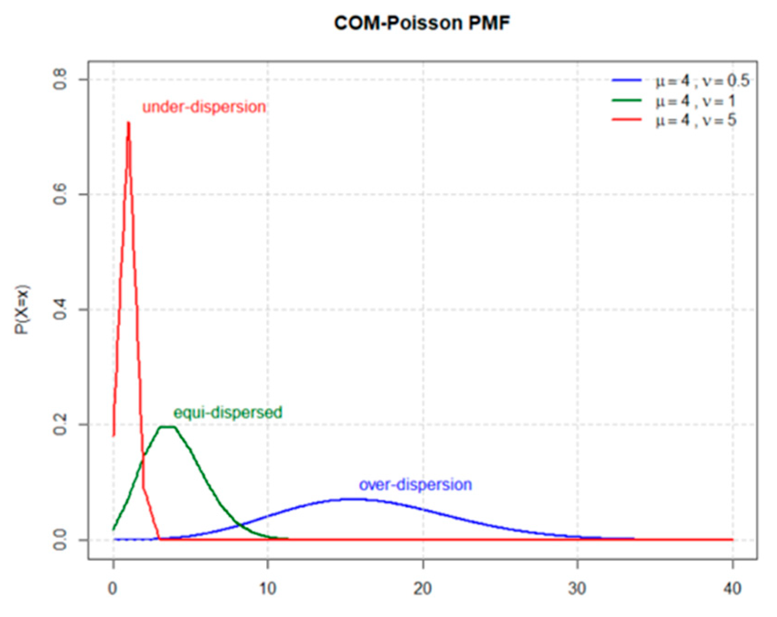
Figure 2.
AQI results of the CMP-EEWMA and MDS-CMP-EEWMA charts.
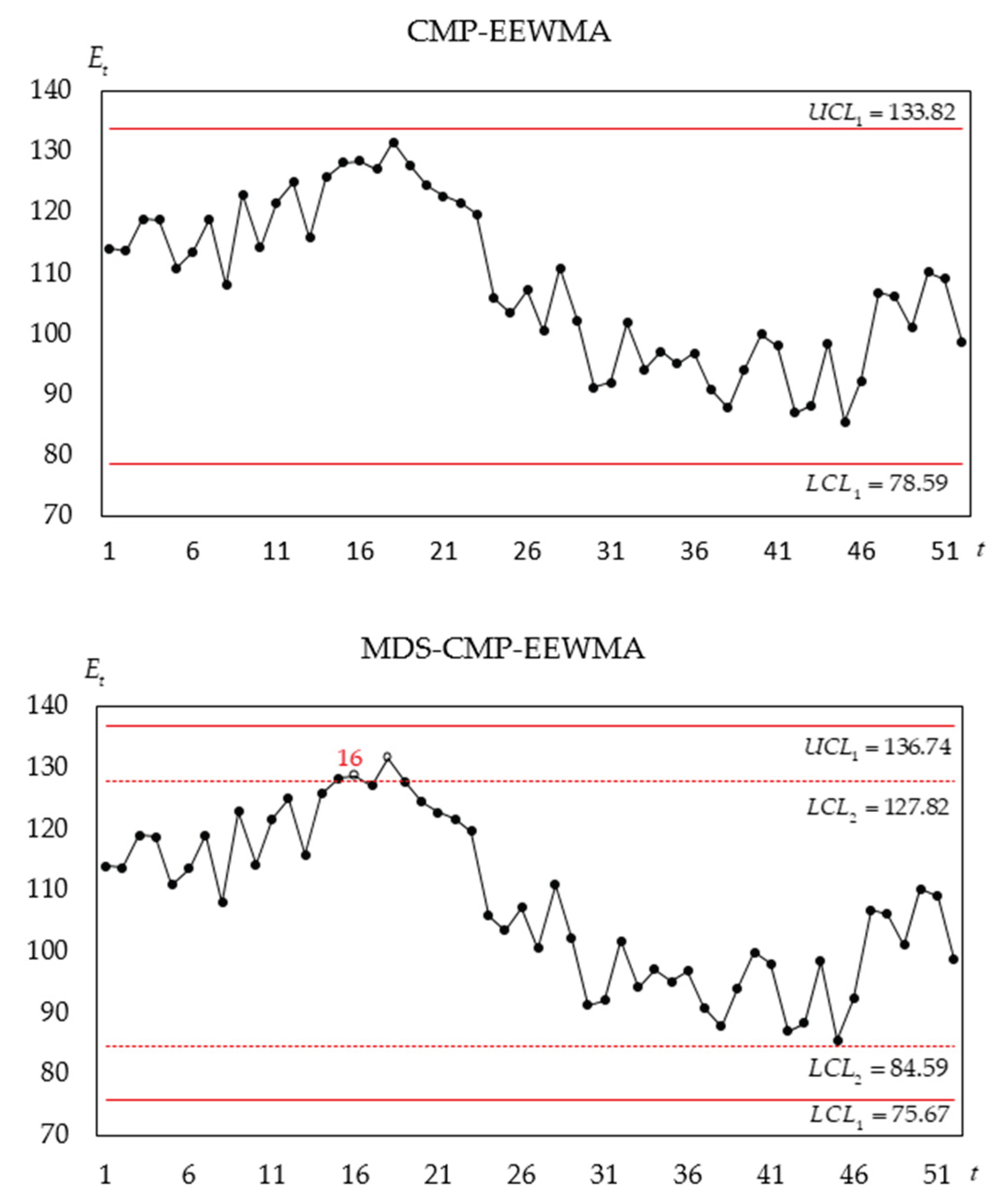

Table 1.
Three probability distributions associated with the COM-Poisson distribution.
| Conditions | Distribution | ||
| , | Geometric | ||
| Poisson | |||
| Bernoulli |
Table 2.
ARL values of the MDS-CMP-EWMA charts using simulation and Aslam et al.’s [14] formula when , and .
Table 2.
ARL values of the MDS-CMP-EWMA charts using simulation and Aslam et al.’s [14] formula when , and .
| ; and | ; and | ||||||||||
| Aslam et.al.’s [14] Formula | Monte Carlo simulation | Aslam et.al.’s [14] Formula | Monte Carlo simulation | ||||||||
| 0.8750 | 1.01 | 3.15 | 16.97 | 15.71 | 1.01 | 2.48 | 15.73 | 13.72 | |||
| 0.9250 | 1.63 | 15.22 | 32.72 | 37.21 | 1.46 | 11.38 | 29.52 | 30.16 | |||
| 0.9375 | 2.47 | 25.16 | 42.11 | 49.70 | 2.06 | 19.49 | 37.45 | 39.35 | |||
| 0.9500 | 4.68 | 42.82 | 57.80 | 68.53 | 3.63 | 35.17 | 50.65 | 52.57 | |||
| 0.9625 | 11.18 | 73.79 | 86.00 | 95.97 | 8.54 | 65.33 | 73.01 | 71.39 | |||
| 0.9750 | 32.92 | 123.82 | 140.01 | 130.29 | 27.03 | 117.89 | 113.60 | 94.37 | |||
| 0.9875 | 106.31 | 183.39 | 226.06 | 157.31 | 100.46 | 182.20 | 173.19 | 113.48 | |||
| 1.0000 | 200.01 | 200.01 | 270.05 | 153.07 | 200.00 | 200.00 | 202.29 | 111.65 | |||
| 1.0125 | 87.22 | 146.03 | 192.72 | 121.85 | 82.07 | 143.72 | 153.18 | 93.23 | |||
| 1.0250 | 24.72 | 82.94 | 116.08 | 88.45 | 20.61 | 78.21 | 97.60 | 70.64 | |||
| 1.0375 | 8.34 | 43.92 | 73.44 | 62.54 | 6.62 | 39.09 | 63.44 | 51.99 | |||
| 1.0500 | 3.67 | 23.70 | 50.13 | 45.37 | 3.00 | 20.03 | 44.71 | 38.45 | |||
| 1.0625 | 2.10 | 13.47 | 37.07 | 33.74 | 1.83 | 11.02 | 33.53 | 29.12 | |||
| 1.0750 | 1.48 | 8.17 | 28.88 | 25.87 | 1.37 | 6.60 | 26.29 | 22.85 | |||
| 1.1250 | 1.01 | 2.14 | 14.72 | 11.79 | 1.01 | 1.87 | 13.78 | 11.02 | |||
Table 3.
The values of the MDS-CMP-EEWMA charts when , , and .
| Scheme | Shift | ||||||||||||
| 0.875 | 0.9625 | 0.9750 | 0.9875 | 1.000 | 1.0125 | 1.0250 | 1.0375 | 1.125 | |||||
| 0 | 2.1852 | - | 15.80 | 70.91 | 109.88 | 171.22 | 200.05 | 148.60 | 93.17 | 60.95 | 13.45 | ||
| 2 | 2.6222 | 1.9929 | 15.94 | 69.87 | 108.26 | 168.10 | 200.00 | 150.53 | 95.43 | 62.07 | 13.93 | ||
| 3 | 3.0592 | 2.0037 | 15.96 | 69.90 | 108.18 | 168.52 | 200.01 | 150.77 | 95.49 | 62.06 | 14.02 | ||
| 4 | 3.4963 | 2.0102 | 15.98 | 69.85 | 108.44 | 169.13 | 200.00 | 150.62 | 95.11 | 61.98 | 14.04 | ||
| 0 | 2.1584 | - | 16.54 | 70.01 | 108.01 | 169.21 | 200.06 | 145.38 | 90.57 | 59.71 | 13.86 | ||
| 2 | 2.5900 | 1.9197 | 16.40 | 67.71 | 104.00 | 164.80 | 200.00 | 148.85 | 93.33 | 61.12 | 14.31 | ||
| 3 | 3.0217 | 1.9352 | 16.42 | 67.64 | 104.09 | 164.46 | 200.05 | 149.03 | 93.34 | 61.10 | 14.42 | ||
| 4 | 3.4534 | 1.9453 | 16.46 | 67.72 | 104.22 | 164.60 | 200.01 | 148.74 | 93.10 | 60.97 | 14.44 | ||
| 0 | 2.1416 | - | 17.92 | 70.65 | 107.55 | 169.25 | 200.01 | 141.37 | 87.42 | 58.34 | 14.40 | ||
| 2 | 2.5699 | 1.8263 | 17.28 | 66.78 | 101.66 | 162.04 | 200.01 | 147.02 | 91.39 | 60.35 | 14.85 | ||
| 3 | 2.9982 | 1.8502 | 17.33 | 66.66 | 101.26 | 161.65 | 200.02 | 147.43 | 91.58 | 60.43 | 15.01 | ||
| 4 | 3.4265 | 1.8680 | 17.40 | 66.93 | 101.83 | 162.38 | 200.03 | 147.02 | 91.23 | 60.39 | 15.04 | ||
| 0 | 2.1871 | - | 21.61 | 77.53 | 114.42 | 175.47 | 200.00 | 136.61 | 84.02 | 57.33 | 15.15 | ||
| 2 | 2.6245 | 1.7175 | 19.38 | 69.72 | 103.61 | 162.38 | 200.02 | 144.65 | 89.34 | 60.20 | 15.47 | ||
| 3 | 3.0619 | 1.7458 | 19.30 | 69.06 | 102.56 | 161.32 | 200.02 | 144.86 | 89.91 | 60.58 | 15.73 | ||
| 4 | 3.4993 | 1.7725 | 19.40 | 69.25 | 102.81 | 161.77 | 200.04 | 143.93 | 89.41 | 60.23 | 15.80 | ||
| 0 | 2.6438 | - | 18.14 | 132.44 | 182.92 | 217.99 | 200.01 | 147.63 | 100.27 | 68.90 | 12.34 | ||
| 2 | 3.1726 | 2.2467 | 16.67 | 111.26 | 160.75 | 204.12 | 200.02 | 153.82 | 105.84 | 72.68 | 12.66 | ||
| 3 | 3.7013 | 2.2562 | 16.51 | 109.96 | 158.36 | 201.75 | 200.02 | 153.96 | 105.81 | 72.54 | 12.82 | ||
| 4 | 4.2301 | 2.2671 | 16.52 | 110.16 | 159.10 | 202.37 | 200.03 | 153.54 | 105.48 | 72.33 | 12.96 | ||
| 0 | 2.6631 | - | 18.03 | 127.39 | 183.70 | 222.05 | 200.00 | 144.14 | 95.75 | 65.20 | 12.28 | ||
| 2 | 3.1957 | 2.1990 | 16.22 | 102.98 | 152.46 | 200.81 | 200.00 | 151.49 | 102.46 | 69.01 | 12.57 | ||
| 3 | 3.7283 | 2.2169 | 16.06 | 101.07 | 150.26 | 199.26 | 200.00 | 152.42 | 103.30 | 69.43 | 12.75 | ||
| 4 | 4.2610 | 2.2338 | 16.10 | 101.24 | 150.40 | 199.97 | 200.04 | 151.55 | 102.36 | 69.03 | 12.88 | ||
| 0 | 2.6899 | - | 18.99 | 124.77 | 184.88 | 227.00 | 200.02 | 137.56 | 90.02 | 61.58 | 12.50 | ||
| 2 | 3.2279 | 2.1268 | 16.41 | 94.54 | 143.62 | 195.10 | 200.01 | 147.56 | 96.79 | 64.95 | 12.68 | ||
| 3 | 3.7659 | 2.1523 | 16.21 | 92.18 | 140.03 | 192.47 | 200.01 | 148.30 | 97.48 | 65.31 | 12.95 | ||
| 4 | 4.3038 | 2.1797 | 16.30 | 92.81 | 140.80 | 195.06 | 200.00 | 147.84 | 96.66 | 64.68 | 13.09 | ||
| 0 | 2.7305 | - | 23.18 | 130.22 | 194.86 | 240.31 | 200.01 | 130.29 | 84.02 | 57.90 | 13.51 | ||
| 2 | 3.2766 | 2.0175 | 18.41 | 90.00 | 136.86 | 193.72 | 200.03 | 141.87 | 90.63 | 61.30 | 13.43 | ||
| 3 | 3.8227 | 2.0523 | 18.11 | 86.98 | 132.88 | 189.82 | 200.03 | 143.96 | 92.61 | 52.16 | 13.80 | ||
| 4 | 4.3688 | 2.2898 | 18.22 | 87.43 | 133.33 | 191.44 | 200.01 | 142.96 | 91.61 | 61.49 | 14.01 | ||
Note: indicating the CMP-EEWMA chart; indicating the MDS-CMP-EEWMA charts.
Table 4.
The values of the MDS-CMP-EEWMA charts when , , and .
| Scheme | Shift | ||||||||||||
| 0.875 | 0.9625 | 0.9750 | 0.9875 | 1.000 | 1.0125 | 1.0250 | 1.0375 | 1.125 | |||||
|
|
|||||||||||||
| 0 | 2.1820 | - | 56.64 | 168.79 | 187.85 | 200.04 | 200.04 | 186.30 | 165.04 | 142.74 | 51.00 | ||
| 2 | 2.6184 | 1.9910 | 55.30 | 163.83 | 184.64 | 198.53 | 200.00 | 187.94 | 168.64 | 146.25 | 52.39 | ||
| 3 | 3.0548 | 2.0003 | 55.29 | 163.60 | 184.52 | 197.96 | 200.01 | 187.12 | 168.23 | 145.97 | 52.29 | ||
| 4 | 3.4912 | 2.0068 | 55.36 | 164.02 | 184.97 | 198.56 | 200.04 | 186.84 | 167.95 | 145.71 | 52.26 | ||
| 0 | 2.1587 | - | 56.55 | 167.48 | 188.56 | 201.19 | 200.00 | 185.45 | 163.20 | 140.54 | 50.13 | ||
| 2 | 2.5904 | 1.9178 | 54.06 | 159.71 | 182.21 | 196.92 | 200.03 | 188.52 | 167.70 | 144.79 | 51.90 | ||
| 3 | 3.0221 | 1.9342 | 54.09 | 159.99 | 182.91 | 197.33 | 200.00 | 188.78 | 167.84 | 145.10 | 51.93 | ||
| 4 | 3.4539 | 1.9440 | 54.19 | 160.18 | 183.11 | 196.73 | 200.02 | 188.13 | 167.49 | 144.56 | 51.75 | ||
| 0 | 2.1434 | - | 58.10 | 168.40 | 190.16 | 203.38 | 200.01 | 182.50 | 159.27 | 135.19 | 48.81 | ||
| 2 | 2.5904 | 1.8282 | 53.96 | 157.16 | 180.09 | 196.71 | 200.00 | 188.11 | 166.69 | 143.37 | 51.40 | ||
| 3 | 3.0221 | 1.8502 | 53.96 | 156.91 | 180.17 | 196.31 | 200.01 | 188.24 | 166.67 | 143.48 | 51.66 | ||
| 4 | 3.4539 | 1.8666 | 54.06 | 157.23 | 180.91 | 196.16 | 200.01 | 187.97 | 165.31 | 142.71 | 51.46 | ||
| 0 | 2.1885 | - | 66.49 | 178.17 | 198.98 | 208.69 | 200.04 | 178.77 | 152.10 | 127.24 | 47.60 | ||
| 2 | 2.6262 | 1.7217 | 57.81 | 158.52 | 182.04 | 197.74 | 200.01 | 186.19 | 162.30 | 138.31 | 50.97 | ||
| 3 | 3.0639 | 1.7438 | 57.11 | 156.63 | 181.01 | 197.15 | 200.02 | 187.26 | 163.20 | 139.42 | 51.37 | ||
| 4 | 3.5016 | 1.7711 | 57.32 | 157.50 | 180.89 | 197.76 | 200.00 | 186.51 | 162.25 | 138.65 | 51.33 | ||
| 0 | 2.6514 | - | 128.13 | 240.94 | 234.34 | 219.02 | 200.04 | 178.84 | 157.09 | 137.71 | 55.23 | ||
| 2 | 3.1817 | 2.2510 | 98.14 | 216.64 | 218.11 | 213.09 | 200.03 | 183.73 | 165.01 | 146.13 | 58.91 | ||
| 3 | 3.7120 | 2.2581 | 95.78 | 214.66 | 216.82 | 211.77 | 200.02 | 183.91 | 165.28 | 146.37 | 58.79 | ||
| 4 | 4.2422 | 2.2692 | 96.03 | 216.42 | 217.81 | 212.30 | 200.01 | 184.44 | 165.33 | 146.08 | 58.54 | ||
| 0 | 2.6713 | - | 122.22 | 246.64 | 237.45 | 221.07 | 200.05 | 176.79 | 152.94 | 132.64 | 52.36 | ||
| 2 | 3.2056 | 2.2052 | 87.88 | 209.72 | 214.94 | 211.29 | 200.01 | 183.93 | 164.20 | 144.12 | 56.27 | ||
| 3 | 3.7398 | 2.1835 | 83.99 | 204.59 | 211.74 | 209.75 | 200.03 | 185.32 | 166.78 | 146.38 | 57.39 | ||
| 4 | 4.2741 | 2.2336 | 85.66 | 208.75 | 214.22 | 210.94 | 200.01 | 183.42 | 164.01 | 144.03 | 55.92 | ||
| 0 | 2.7024 | - | 121.64 | 258.98 | 247.05 | 225.85 | 200.01 | 172.78 | 147.59 | 125.84 | 49.14 | ||
| 2 | 3.2429 | 2.1352 | 79.52 | 204.40 | 212.43 | 210.62 | 200.03 | 182.98 | 161.51 | 139.81 | 52.99 | ||
| 3 | 3.7834 | 2.1533 | 76.48 | 200.42 | 209.54 | 210.16 | 200.01 | 182.19 | 161.66 | 140.94 | 53.50 | ||
| 4 | 4.3238 | 2.1783 | 77.30 | 202.06 | 210.85 | 210.15 | 200.01 | 181.70 | 160.30 | 139.62 | 53.06 | ||
| 0 | 2.7553 | - | 136.25 | 293.93 | 268.67 | 235.34 | 200.04 | 167.59 | 140.75 | 119.00 | 46.88 | ||
| 2 | 3.3064 | 2.0247 | 75.81 | 203.94 | 213.68 | 213.17 | 200.04 | 179.96 | 155.51 | 133.17 | 50.09 | ||
| 3 | 3.8574 | 2.0501 | 72.93 | 197.84 | 210.21 | 211.00 | 200.03 | 180.04 | 157.08 | 134.62 | 50.75 | ||
| 4 | 4.4085 | 2.0867 | 73.58 | 200.01 | 212.39 | 212.09 | 200.01 | 179.30 | 156.89 | 133.22 | 50.54 | ||
Note: indicating the CMP-EEWMA chart; indicating the MDS-CMP-EEWMA charts.
Table 5.
The values of the MDS-CMP-EEWMA charts when , , and .
| Scheme | Shift | |||||||||||||
| 0.875 | 0.9625 | 0.9750 | 0.9875 | 1.000 | 1.0125 | 1.0250 | 1.0375 | 1.125 | ||||||
|
|
||||||||||||||
| 0 | 2.2600 | - | 148.10 | 189.42 | 193.95 | 197.60 | 200.04 | 201.12 | 201.39 | 202.40 | 182.05 | |||
| 2 | 2.7120 | 1.9944 | 150.32 | 190.57 | 194.66 | 198.01 | 200.04 | 200.63 | 200.77 | 200.74 | 178.78 | |||
| 3 | 3.1640 | 2.0081 | 149.87 | 190.53 | 194.55 | 198.09 | 200.01 | 200.47 | 201.02 | 201.25 | 179.86 | |||
| 4 | 3.6160 | 2.0235 | 148.73 | 190.04 | 194.14 | 198.01 | 200.02 | 200.82 | 201.29 | 201.88 | 181.18 | |||
| 0 | 2.2475 | - | 146.72 | 189.72 | 193.56 | 197.30 | 200.00 | 201.24 | 201.39 | 201.94 | 178.10 | |||
| 2 | 2.6970 | 1.8870 | 145.23 | 189.48 | 193.40 | 196.90 | 200.01 | 201.52 | 202.27 | 202.93 | 180.59 | |||
| 3 | 3.1465 | 1.9219 | 144.16 | 188.22 | 192.66 | 197.00 | 200.01 | 202.12 | 203.16 | 203.60 | 183.06 | |||
| 4 | 3.5960 | 1.9469 | 142.57 | 187.91 | 192.78 | 196.81 | 200.01 | 202.31 | 203.64 | 204.27 | 183.50 | |||
| 0 | 2.2475 | - | 146.10 | 190.64 | 194.29 | 197.93 | 200.02 | 201.54 | 201.01 | 200.77 | 173.23 | |||
| 2 | 2.6970 | 1.8870 | 138.77 | 186.54 | 191.84 | 196.02 | 200.02 | 202.88 | 204.28 | 205.35 | 186.05 | |||
| 3 | 3.1465 | 1.9219 | 137.45 | 185.86 | 191.03 | 196.29 | 200.03 | 202.42 | 203.76 | 205.40 | 186.55 | |||
| 4 | 3.5960 | 1.9469 | 137.58 | 186.24 | 191.09 | 196.48 | 200.00 | 202.54 | 203.58 | 205.16 | 185.37 | |||
| 0 | 2.2098 | - | 151.00 | 191.66 | 195.03 | 198.01 | 200.02 | 200.69 | 199.23 | 197.34 | 165.74 | |||
| 2 | 2.6518 | 1.8737 | 140.03 | 187.13 | 192.58 | 197.12 | 200.03 | 202.44 | 202.91 | 203.44 | 181.94 | |||
| 3 | 3.0937 | 1.9072 | 139.16 | 186.76 | 192.02 | 196.08 | 200.00 | 202.31 | 203.31 | 203.95 | 181.00 | |||
| 4 | 3.5357 | 1.9377 | 140.58 | 187.75 | 192.44 | 196.77 | 200.02 | 202.99 | 203.87 | 204.19 | 179.48 | |||
| 0 | 2.7786 | - - | 173.20 | 196.84 | 198.77 | 199.23 | 200.00 | 200.33 | 200.26 | 199.58 | 182.33 | |||
| 2 | 3.3343 | 2.2554 | 158.19 | 190.71 | 194.72 | 197.14 | 200.05 | 202.62 | 204.70 | 205.99 | 201.22 | |||
| 3 | 3.8900 | 2.3090 | 158.52 | 191.06 | 194.78 | 197.27 | 200.00 | 202.28 | 203.76 | 205.00 | 200.09 | |||
| 4 | 4.4458 | 2.3282 | 161.60 | 192.23 | 195.61 | 197.74 | 200.02 | 201.70 | 202.66 | 203.39 | 195.38 | |||
| 0 | 2.7625 | - | 174.37 | 197.82 | 199.00 | 199.15 | 200.06 | 199.58 | 198.58 | 197.51 | 176.54 | |||
| 2 | 3.3150 | 2.2652 | 154.64 | 189.99 | 193.92 | 196.58 | 200.04 | 202.31 | 204.18 | 205.30 | 200.47 | |||
| 3 | 3.8675 | 2.3241 | 153.50 | 190.19 | 194.30 | 196.80 | 200.01 | 202.17 | 204.29 | 205.07 | 199.64 | |||
| 4 | 4.4200 | 2.3481 | 155.94 | 191.10 | 195.17 | 197.17 | 200.03 | 201.71 | 203.32 | 204.29 | 195.67 | |||
| 0 | 2.7204 | - | 178.98 | 201.27 | 200.84 | 200.54 | 200.00 | 199.12 | 196.74 | 194.65 | 167.24 | |||
| 2 | 3.2645 | 2.2908 | 154.94 | 191.67 | 195.32 | 197.60 | 200.04 | 201.68 | 201.63 | 201.69 | 189.31 | |||
| 3 | 3.8086 | 2.3333 | 153.99 | 191.21 | 194.86 | 197.39 | 200.02 | 200.89 | 201.40 | 202.05 | 188.66 | |||
| 4 | 4.3526 | 2.3611 | 154.55 | 190.97 | 194.80 | 197.42 | 200.00 | 200.94 | 201.65 | 202.30 | 187.27 | |||
| 0 | 2.5910 | - | 183.72 | 204.92 | 204.98 | 203.63 | 200.02 | 197.68 | 193.44 | 190.06 | 154.37 | |||
| 2 | 3.1092 | 2.2955 | 160.77 | 194.19 | 197.04 | 198.34 | 200.01 | 200.02 | 199.07 | 198.22 | 174.18 | |||
| 3 | 3.6274 | 2.3058 | 159.86 | 193.96 | 197.05 | 198.70 | 200.05 | 199.14 | 198.15 | 197.02 | 170.46 | |||
| 4 | 4.1456 | 2.3167 | 157.68 | 193.77 | 196.83 | 198.53 | 200.02 | 199.25 | 198.33 | 196.78 | 169.79 | |||
Note: indicating the CMP-EEWMA chart; indicating the MDS-CMP-EEWMA charts.
Table 6.
Comparisons among the MDS-CMP-EEWMA, MDS-CMP-EWMA, CMP-EEWMA, and CMP-EWMA charts when at and .
Table 6.
Comparisons among the MDS-CMP-EEWMA, MDS-CMP-EWMA, CMP-EEWMA, and CMP-EWMA charts when at and .
| Scheme | Shift | ||||||||||||
| 0.875 | 0.9625 | 0.9750 | 0.9875 | 1.000 | 1.0125 | 1.0250 | 1.0375 | 1.125 | |||||
| , | |||||||||||||
| 0(CMP-EWMA) | 2.2177 | - | 15.41 | 73.24 | 113.75 | 172.78 | 200.03 | 151.02 | 95.59 | 62.55 | 13.22 | ||
| 2(MDS-CMP-EWMA) | 2.6612 | 2.0517 | 15.67 | 72.60 | 112.72 | 170.85 | 200.01 | 151.90 | 96.83 | 63.09 | 13.66 | ||
| 3(MDS-CMP-EWMA) | 3.1048 | 2.0593 | 15.68 | 72.60 | 112.70 | 171.33 | 200.00 | 151.78 | 96.88 | 63.12 | 13.75 | ||
| 4(MDS-CMP-EWMA) | 3.5483 | 2.0632 | 15.68 | 72.57 | 112.66 | 171.51 | 200.01 | 151.68 | 96.78 | 63.04 | 13.76 | ||
| , | |||||||||||||
| 0(CMP-EEWMA) | 2.1416 | - | 17.92 | 70.65 | 107.55 | 169.25 | 200.01 | 141.37 | 87.42 | 58.34 | 14.40 | ||
| 2(MDS-CMP-EEWMA) | 2.5699 | 1.8263 | 17.28 | 66.78 | 101.66 | 162.04 | 200.01 | 147.02 | 91.39 | 60.35 | 14.85 | ||
| 3(MDS-CMP-EEWMA) | 2.9982 | 1.8502 | 17.33 | 66.66 | 101.26 | 161.65 | 200.02 | 147.43 | 91.58 | 60.43 | 15.01 | ||
| 4(MDS-CMP-EEWMA) | 3.4265 | 1.8680 | 17.40 | 66.93 | 101.83 | 162.38 | 200.03 | 147.02 | 91.23 | 60.39 | 15.04 | ||
| , | |||||||||||||
| 0(CMP-EWMA) | 2.2135 | - | 58.17 | 170.99 | 189.94 | 201.50 | 200.02 | 186.14 | 167.01 | 144.95 | 52.00 | ||
| 2(MDS-CMP-EWMA) | 2.6562 | 2.0506 | 57.43 | 169.52 | 189.13 | 200.55 | 200.03 | 188.21 | 169.05 | 147.56 | 52.98 | ||
| 3(MDS-CMP-EWMA) | 3.0989 | 2.0573 | 57.33 | 168.89 | 188.94 | 200.19 | 200.00 | 187.55 | 168.76 | 147.21 | 52.91 | ||
| 4(MDS-CMP-EWMA) | 3.5416 | 2.0606 | 57.25 | 168.70 | 188.78 | 200.04 | 200.00 | 187.31 | 168.71 | 146.96 | 52.83 | ||
| , | |||||||||||||
| 0(CMP-EEWMA) | 2.1434 | - | 58.10 | 168.40 | 190.16 | 203.38 | 200.01 | 182.50 | 159.27 | 135.19 | 48.81 | ||
| 2(MDS-CMP-EEWMA) | 2.5904 | 1.8282 | 53.96 | 157.16 | 180.09 | 196.71 | 200.00 | 188.11 | 166.69 | 143.37 | 51.40 | ||
| 3(MDS-CMP-EEWMA) | 3.0221 | 1.8502 | 53.96 | 156.91 | 180.17 | 196.31 | 200.01 | 188.24 | 166.67 | 143.48 | 51.66 | ||
| 4(MDS-CMP-EEWMA) | 3.4539 | 1.8666 | 54.06 | 157.23 | 180.91 | 196.16 | 200.01 | 187.97 | 165.31 | 142.71 | 51.46 | ||
| , | |||||||||||||
| 0(CMP-EWMA) | 2.2637 | - | 148.47 | 189.45 | 193.56 | 196.86 | 200.01 | 201.07 | 201.47 | 202.79 | 185.55 | ||
| 2(MDS-CMP-EWMA) | 2.7164 | 2.1004 | 152.85 | 191.46 | 194.84 | 197.88 | 200.00 | 200.89 | 201.57 | 201.73 | 180.75 | ||
| 3(MDS-CMP-EWMA) | 3.1692 | 2.1034 | 152.73 | 191.53 | 194.78 | 197.63 | 200.01 | 200.74 | 201.46 | 201.90 | 180.87 | ||
| 4(MDS-CMP-EWMA) | 3.6219 | 2.1116 | 151.42 | 191.00 | 194.25 | 197.26 | 200.01 | 200.84 | 201.35 | 201.81 | 181.65 | ||
| , | |||||||||||||
| 0(CMP-EEWMA) | 2.2282 | - | 146.10 | 190.64 | 194.29 | 197.93 | 200.02 | 201.54 | 201.01 | 200.77 | 173.23 | ||
| 2(MDS-CMP-EEWMA) | 2.6738 | 1.8432 | 138.77 | 186.54 | 191.84 | 196.02 | 200.02 | 202.88 | 204.28 | 205.35 | 186.05 | ||
| 3(MDS-CMP-EEWMA) | 3.1195 | 1.8921 | 137.45 | 185.86 | 191.03 | 196.29 | 200.03 | 202.42 | 203.76 | 205.40 | 186.55 | ||
| 4(MDS-CMP-EEWMA) | 3.5651 | 1.9262 | 137.58 | 186.24 | 191.09 | 196.48 | 200.00 | 202.54 | 203.58 | 205.16 | 185.37 | ||
Table 8.
The CMP-EEWMA and MDS-CMP-EEWMA Charts for monitoring weekly AQI count data for Zhongli in 2025.
Table 8.
The CMP-EEWMA and MDS-CMP-EEWMA Charts for monitoring weekly AQI count data for Zhongli in 2025.
| Week | Week | Week | Week | ||||||||
| 1 | 145 | 113.9665 | 14 | 159 | 125.6912 | 27 | 44 | 100.4842 | 40 | 119 | 99.8442 |
| 2 | 137 | 113.6078 | 15 | 165 | 128.2236 | 28 | 107 | 110.8248 | 41 | 106 | 98.0105 |
| 3 | 159 | 118.9435 | 16 | 159 | 128.4946 | 29 | 64 | 102.0718 | 42 | 49 | 86.9300 |
| 4 | 150 | 118.7458 | 17 | 146 | 127.1148 | 30 | 17 | 91.1489 | 43 | 63 | 88.2128 |
| 5 | 104 | 110.7959 | 18 | 164 | 131.4703 | 31 | 36 | 91.9830 | 44 | 119 | 98.4043 |
| 6 | 119 | 113.5241 | 19 | 138 | 127.5714 | 32 | 96 | 101.7437 | 45 | 50 | 85.4281 |
| 7 | 145 | 118.9431 | 20 | 120 | 124.3886 | 33 | 59 | 94.1139 | 46 | 91 | 92.2110 |
| 8 | 85 | 107.9854 | 21 | 112 | 122.6130 | 34 | 81 | 97.1094 | 47 | 164 | 106.7626 |
| 9 | 164 | 122.8660 | 22 | 109 | 121.5885 | 35 | 74 | 95.0650 | 48 | 149 | 106.0521 |
| 10 | 112 | 114.1114 | 23 | 102 | 119.6850 | 36 | 87 | 96.8224 | 49 | 115 | 100.9700 |
| 11 | 150 | 121.6269 | 24 | 36 | 105.7776 | 37 | 59 | 90.8295 | 50 | 158 | 110.1312 |
| 12 | 161 | 124.9618 | 25 | 38 | 103.3865 | 38 | 50 | 87.7563 | 51 | 143 | 109.0459 |
| 13 | 108 | 115.8034 | 26 | 70 | 107.1710 | 39 | 89 | 94.0461 | 52 | 84 | 98.6041 |
Disclaimer/Publisher’s Note: The statements, opinions and data contained in all publications are solely those of the individual author(s) and contributor(s) and not of MDPI and/or the editor(s). MDPI and/or the editor(s) disclaim responsibility for any injury to people or property resulting from any ideas, methods, instructions or products referred to in the content. |
© 2026 by the authors. Licensee MDPI, Basel, Switzerland. This article is an open access article distributed under the terms and conditions of the Creative Commons Attribution (CC BY) license (http://creativecommons.org/licenses/by/4.0/).
Copyright: This open access article is published under a Creative Commons CC BY 4.0 license, which permit the free download, distribution, and reuse, provided that the author and preprint are cited in any reuse.


