

Submitted:
25 June 2026
Posted:
25 June 2026
You are already at the latest version
Abstract
After analyzing the behavior of the control object based on linear theory, and calculating the necessary control laws, when implementing systems based on the calculations performed, you may encounter some discrepancies between the reactions received from the real object and the expected ones. The properties of the assembled system, built on real elements, can differ significantly from the calculated ones.So in a stable, according to a linear model, system, undamped oscillations can be observed. A small error in the processing of input actions in the linear model turns out to be much larger or even increases indefinitely. The transient process in a real system can be much longer than in a linear case. An astatic system in a linear approximation can in reality work out actions with a constant steady-state error. The reason for all these phenomena is the discrepancy between the properties of real elements and their linear model adopted in the calculation.
Keywords:
acceleration of the mechanism
; Heaviside function
; non-linear system
; Matlab
1. Introduction
The purpose of this work is to observe the dependence of the response of a system previously calculated using a linear model to typical actions if they are applied not to a model linear system, but to a real object containing nonlinear elements.
The object of research is a mobile radar antenna. The purpose of object control is to maintain a constant angular velocity of the antenna. Typical impacts on the system are selected based on the characteristics of the object and its scope. Among the operating modes of the object are long-term observation of the entire surrounding space (continuous rotation of the antenna) and observation of a certain sector (periodic rotational movements of an oscillatory nature). Short-term impacts of large amplitude and high-frequency impacts of small amplitude can be applied to the input of the object due to the features of the line that supplies the input signal to the system. Periodic oscillatory effects can be applied to the antenna from the outside, this is due to the specifics of the location of the control object on the ground.
2. Method Research
2.1. Setting Tasks
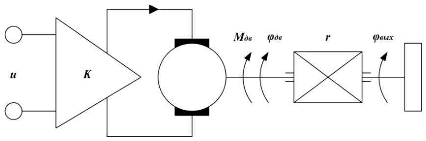
It was necessary to synthesize the control law for the acceleration system of the inertial rotor. It was required to ensure the process of acceleration to a given constant speed, providing a given quality of transient processes in terms of speed, oscillation and overshoot.
Figure 1.
Functional diagram of the installation.
2.2. Design Scheme
First, it was necessary to build an adequate model of a real system and introduce its parameters:
Figure 2.
Control object scheme.
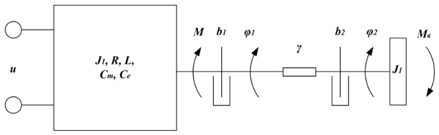
It was believed that only the first natural frequency is important in the operating frequency range. For the study, the values of the system parameters were set. The control object is a radar antenna mounted on a movable base. The accepted values are given in the table:

Table 1.
Please add caption.
| Value name | Designation | Meaning | Unit dimensions |
|---|---|---|---|
| The upper limit of the frequency range of processed actions | 20 | 1/s | |
| Natural frequency of the system | 8 | 1/s | |
| Reduced moment of inertia of the motor | 2,25 | Kg.m2 | |
| Reduced load moment of inertia | 2 | Kg.m2 | |
| Reduced coefficient of viscous friction of the input shaft | 1,7 | N∙m∙s | |
| Output shaft viscous friction coefficient | 3,4 | N∙m∙s | |
| Electrical analogue of viscosity | 3,4 | N∙m∙s | |
| Rigidity of the kinematic transmission | 67,76471 | N∙m | |
| Reduced electromechanical gain | 45 | N∙m/V | |
| Characteristic time of electrical processes | 0,01 | s |
2.3. Mathematical Models of the Control Object
In this problem, the input is the control voltage and the external disturbing moment , the output is the angular velocity of the output shaft. Let’s write down the system of differential equations describing the behavior of the object:
In this system: , , .
Because , that is, electrical processes in the system proceed much faster than mechanical ones , in the third equation the first term was taken out of consideration. The system has been rewritten as:
Having additionally adopted the notation , we write the system of equations as follows:
2.4. Regulator Synthesis
For the system described above, using the compensation method, a controller was synthesized, the transfer function of which is given below:
It was assumed that the block diagram of a closed system has the form:
Figure 3.
Closed system diagram.
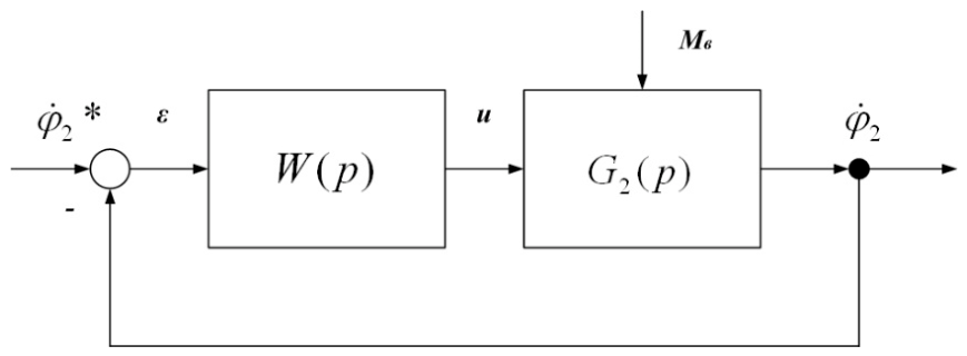
In the diagram- the transfer function from the inputs (control voltage and external torque ) to the angular velocity of the output shaft (antenna) .
It makes sense to apply the following typical actions to the system input:
- Heaviside function (observation mode for the entire surrounding space);
- sinusoidal action of low frequency and high amplitude (sector monitoring mode);
A signal is selected as a sinusoidal input signal of low frequency and high amplitude . High frequency signal-.
As mentioned earlier, in the case of assembling a system designed according to a linear model from real elements, its properties may differ from those expected- the response to input actions may be different. Moreover, the differences can be of a qualitative nature.
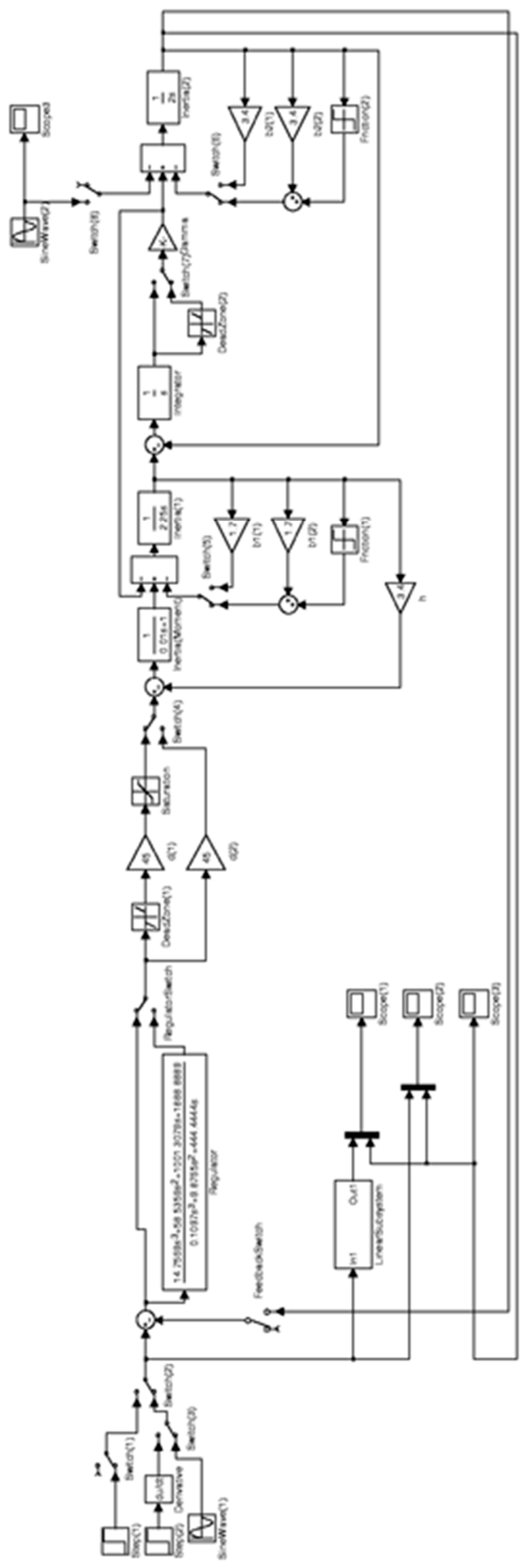
In this section, we will check the response of the object to the inclusion of non-linearities in it. The verification will be carried out at different levels of nonlinearities according to the reaction of the resulting system to the input of the Heaviside function to the input of the system.
2.5. Description of the Types of Nonlinearities
First of all, it makes sense to consider in more detail the types of nonlinearities that take place in a given system.
2.5.1. Dead Zone
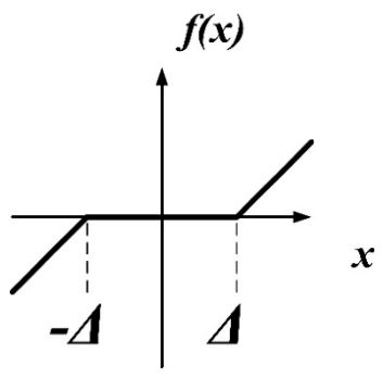
This nonlinear dependence will be used in the description of the amplifier and kinematic gears. In the case of an amplifier, this dependence means that there is a minimum threshold voltage, only when it is exceeded, a non-zero signal appears at the output. When describing kinematic gears, this dependence makes it possible to take into account gaps. An example of this relationship is shown in the graph below.
Figure 4.
Approximate view of the dependence of the “dead zone” type.
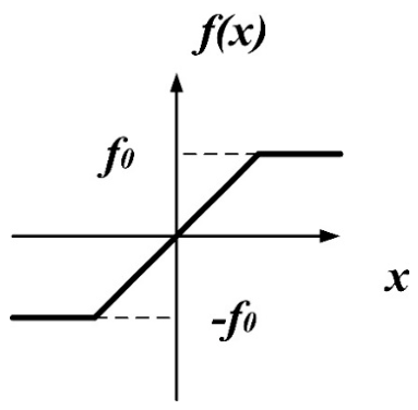
2.5.2. Saturation (Limitation)
This nonlinear dependence will be used in the description of the amplifier. With its help, you can take into account the limitations of the output signal. An example of this dependence is shown in the graph below.
Figure 5.
Approximate type of dependence of the “saturation” type.
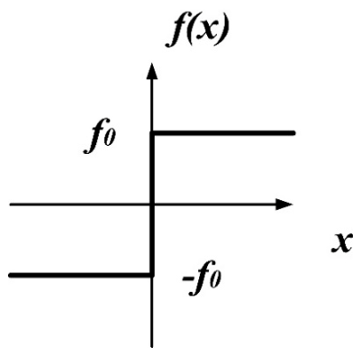
2.5.3. Coulomb Friction (Relay)
This type of non-linear dependence makes it possible to describe the effect of Coulomb friction. An example of this relationship is shown in the graph below.
Figure 6.
Approximate type of “relay” dependency.
2.5.4. Friction with Stribeck Effect (Friction Model)
This type of nonlinear dependence corresponds to the Stribeck friction model. The peculiarity of this model is that at the beginning of the movement, the friction moment first decreases, starting from the static friction moment, and then begins to increase nonlinearly with an increase in the speed of movement. An approximate view of this non-linear dependence is shown in the graph below.
3. Results and Discussions
3.1. Heaviside Function
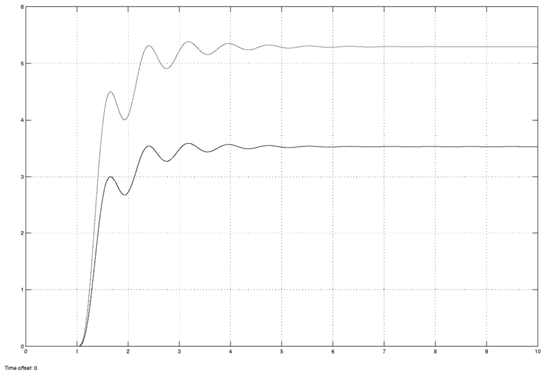
It can be seen from the graphs that the linear model describes the processes occurring in the system quite well in terms of the oscillation and time of the transient process. The output signal of a linear model is larger in magnitude (uniformly in time) compared to the signal of a non-linear system, which leads to an increase in overshoot in it.
Thus, there are no qualitative differences between the response of a nonlinear system and a linear system to given actions in this case.
3.1.1. Amplifier. Saturation
To test the influence of this type of nonlinearity in a given system, we also simulated the system’s response to the input of the Heaviside function to its input. The simulation was carried out with the values .
In the graphs below: the light curve is a linear system, the dark curve is a non-linear system.
Figure 7.
Response of systems to the Heaviside function ().
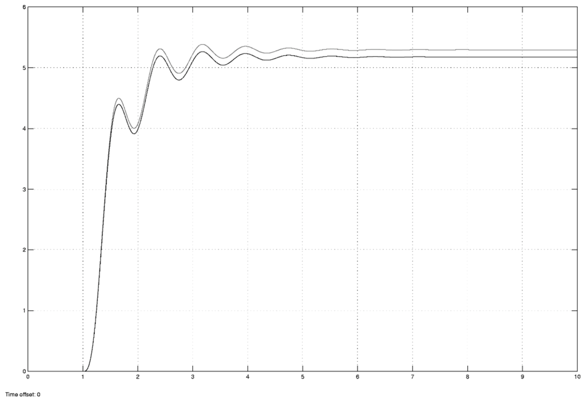
Figure 8.
Response of systems to the Heaviside function ().
3.2. Heaviside Function
From the graphs, it is obvious that in this case, as in the previous one, the linear model describes the processes occurring in the system quite well in terms of oscillation and transient time. The amount of overshoot in the linear case is greater than in the non-linear one. This is due to the fact that the signal of the linear model is larger in magnitude compared to the non-linear system (similar to the previous case).
The use of a linear model does not introduce qualitative changes in the system’s response to typical impacts.
3.2.1. Coulomb Friction
First bearing. Now let’s consider how the Coulomb friction in the first bearing will affect the output signal of the system. For modeling, the following final values of the Coulomb friction coefficient were chosen- (this set is the same when both considered functions are fed to the input).
In the graphs below: the light curve is a linear curve, the dark curve is a non-linear system.
Figure 9.
The response of systems to the Heaviside function (friction coefficient- ).
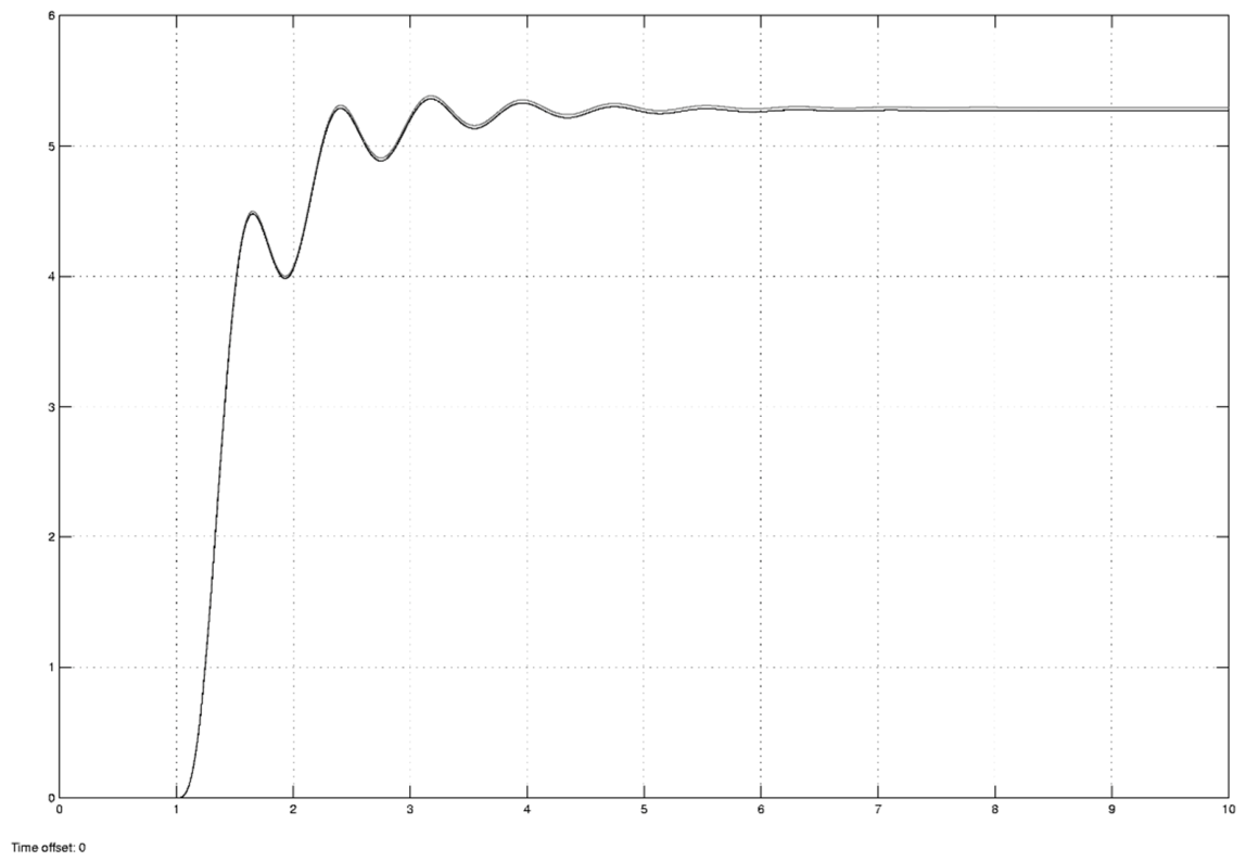
Figure 10.
The response of systems to the Heaviside function (friction coefficient- ).
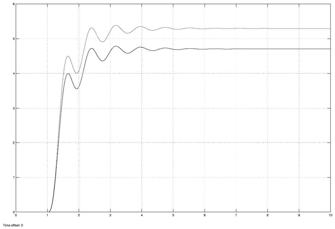
3.2.2. Coulomb Friction
Second bearing. Let us introduce into consideration the Coulomb friction in the second bearing with its final value equal to. We will proceed similarly to the previous case.
In the graphs below, the light curve is a linear system, the dark curve is a non-linear system).
Figure 11.
The response of systems to the Heaviside function (friction coefficient- )
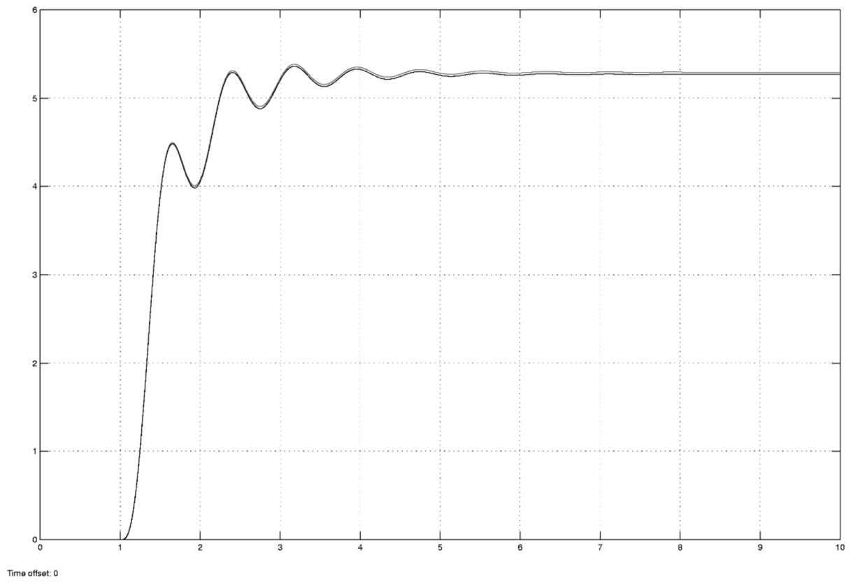
Figure 12.
The response of systems to the Heaviside function (friction coefficient- )
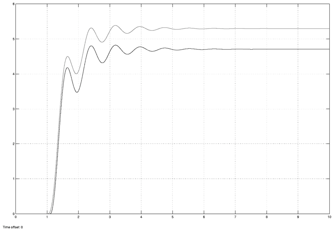
It can be seen from the graphs that the changes are noticeable only in the amount of overshoot. This is due to the time-uniform difference in the magnitudes of the output signals of the linear and nonlinear systems.
Thus, in this case, there are no qualitative differences between the reactions of the nonlinear and linear systems.
4. Conclusion
In this work, we compared the performance of two models of a real system, linear and non-linear. To simulate the processes occurring in both systems, the Simulink software package was used. Based on the results of the research, it can be concluded that a linear system is only an approximation to a real object and in fact allows you to reproduce only a small part of the effects that take place in a real nonlinear system.
A study was also made of the phenomenon of capture by a nonlinear system of forced oscillations. It was possible to observe the occurrence of forced oscillations in the system under the action of a harmonic driving force of a certain amplitude in a certain frequency range.
References
- Pervozvanski, A. A. Course in Automatic Control Theory; Nauka, 2006. [Google Scholar]
- Dorf, R. C.; Bishop, R. H. Modern Control Systems; Laboratory of Basic Knowledge, 2004. [Google Scholar]
- Preumont, A. Vibration Control of Active Structures: An Introduction, 3rd ed.; Springer, 2011. [Google Scholar]
- Gawronski, W. K. Advanced Structural Dynamics and Active Control of Structures; Springer, 2004. [Google Scholar]
- Bolton, W. Mechatronics: Electronic Control Systems in Mechanical and Electrical Engineering, 6th ed.; Pearson, 2015. [Google Scholar]
- Alciatore, D. G.; Histand, M. B. Introduction to Mechatronics and Measurement Systems, 4th ed.; McGraw-Hill, 2012. [Google Scholar]
- de Silva, C. W. Mechatronics: An Integrated Approach; CRC Press, 2009. [Google Scholar]
- Fuller, C. R.; Elliott, S. J.; Nelson, P. A. Active Control of Vibration; Academic Press, 1996. [Google Scholar]
- Inman, D. J. Vibration with Control; John Wiley & Sons, 2006. [Google Scholar]
- Jouaneh, M. Fundamentals of Mechatronics; Cengage Learning, 2012. [Google Scholar]
- Kuo, B. C.; Golnaraghi, F. Automatic Control Systems, 9th ed.; John Wiley & Sons, 2010. [Google Scholar]
- Nise, N. S. Control Systems Engineering, 7th ed.; John Wiley & Sons, 2015. [Google Scholar]
- Cetinkunt, S. Mechatronics; John Wiley & Sons, 2007. [Google Scholar]
- Lyshevski, S. E. Electromechanical Systems and Devices; CRC Press, 2008. [Google Scholar]
- Preumont, A. Vibration Control of Active Structures: An Introduction, 4th ed.; Springer, 2018. [Google Scholar]
- Bishop, R. H. (Ed.) The Mechatronics Handbook, 2nd ed.; CRC Press, 2007. [Google Scholar]
- Onwubolu, G. C. Mechatronics: Principles and Applications; Elsevier Butterworth-Heinemann, 2005. [Google Scholar]
- Huu-Dien, Nguyen; Shyh-Chour, Huang. Using the Extended Finite Element Method to Integrate the Level-Set Method to Simulate the Stress Concentration Factor at the Circular Holes Near the Material Boundary of a Functionally-Graded Material Plate. JMR&T 2022, 21C 4658–4673. [Google Scholar]
- Nguyen, H.-D.; Huang, S.-C. Use of XTFEM based on the consecutive interpolation procedure of quadrilateral element to calculate J-integral and SIFs of an FGM plate. Theor. Appl. Fract. Mech. 2023, 127, 103985. [Google Scholar] [CrossRef]
Disclaimer/Publisher’s Note: The statements, opinions and data contained in all publications are solely those of the individual author(s) and contributor(s) and not of MDPI and/or the editor(s). MDPI and/or the editor(s) disclaim responsibility for any injury to people or property resulting from any ideas, methods, instructions or products referred to in the content. |
© 2026 by the authors. Licensee MDPI, Basel, Switzerland. This article is an open access article distributed under the terms and conditions of the Creative Commons Attribution (CC BY) license (http://creativecommons.org/licenses/by/4.0/).
Copyright: This open access article is published under a Creative Commons CC BY 4.0 license, which permit the free download, distribution, and reuse, provided that the author and preprint are cited in any reuse.