

Submitted:
25 June 2026
Posted:
25 June 2026
You are already at the latest version
Abstract
This study analyzes long memory, multifractality and forecasting performance in coffee, Brent oil and gold futures, three international commodity markets of strategic relevance for Colombia. Daily futures prices from 2016 to 2025 were examined using logarithmic returns, descriptive statistics, rolling volatility, Hurst R/S, detrended fluctuation analysis (DFA), multifractal detrended fluctuation analysis (MF-DFA), out-of-sample forecasting models, conditional volatility models and Monte Carlo simulation. The results show heterogeneous long-memory evidence across commodities and market regimes. R/S estimates suggested persistence in the three markets, while DFA moderated this conclusion. MF-DFA confirmed multifractal behavior in all series, with gold and Brent showing wider heterogeneity than coffee. Forecasting results showed that simple models, particularly random walk and drift specifications, were difficult to outperform in one-step-ahead predictions. Monte Carlo simulations generated probabilistic price scenarios for 30-, 60- and 90-trading-day horizons, and an ex-post validation with 2026 observed prices showed that six of nine realized prices fell within the simulated P5-P95 intervals. Overall, the findings suggest that commodity futures relevant to Colombia exhibit differentiated forms of temporal complexity, risk and scenario uncertainty that cannot be fully captured by linear models or average volatility measures.
Keywords:
commodity futures
; coffee
; oil
; gold
; Hurst exponent
; long memory
; multifractality
; MF-DFA
; fractional modeling
; Monte Carlo simulation
1. Introduction
Commodity futures markets play a central role in expectation formation, price discovery, risk management and hedging strategies within international agricultural, energy and financial systems. These markets concentrate information on supply, demand, inventories, macroeconomic conditions, geopolitical tensions, climate shocks, financial expectations and the global perception of risk. Recent literature has shown that commodity markets may exhibit time-varying efficiency, temporal memory, persistent volatility and multifractal structures that change according to the asset, the time scale and crisis episodes [1,2,3,4]. Within this context, coffee, Brent oil and gold futures constitute three markets of particular interest, not only because of their international relevance, but also because they incorporate information and uncertainty in differentiated ways.
Although the three assets are classified as commodities, their economic fundamentals differ. Coffee represents an agricultural commodity exposed to weather conditions, crop cycles, inventories, supply-related constraints, logistical pressures and changes in international demand. Brent oil is positioned as a global energy benchmark sensitive to production decisions, geopolitical tensions, abrupt supply variations, demand expectations and macroeconomic conditions. Gold has a particular financial nature, since it frequently operates as a safe-haven asset during periods of uncertainty, inflation, risk aversion or market instability. This diversity makes it possible to analyze whether commodity futures display similar patterns of memory, persistence and temporal complexity, or whether each market exhibits different statistical structures.
For Colombia, the study of these commodities is highly relevant because they are strategic assets linked to different economic channels. Coffee is a historical export agricultural product with territorial relevance; oil is associated with external revenues, fiscal accounts, royalties, extractive investment, the trade balance and macroeconomic sensitivity; and gold is important for the mining sector, foreign-exchange generation and the interpretation of financial risk. This study does not analyze Colombian domestic prices or directly estimate the impact of these commodities on national macroeconomic variables. The empirical analysis focuses on international futures prices because these markets serve as global benchmarks for expectation formation, hedging, risk valuation and price-scenario anticipation.
From this perspective, studying long memory, multifractality and forecasting performance in coffee, Brent and gold futures provides contextual evidence on the external uncertainty faced by commodities that are strategic for Colombia. The central question is not whether international prices by themselves explain national economic dynamics, but whether these markets contain complex temporal structures that may affect the interpretation of risk, the construction of scenarios and decision-making in economies exposed to these commodities.
Traditionally, the modeling of financial and commodity prices has often relied on assumptions of weak-form efficiency, temporal independence, approximate normality and short-term dependence. However, in speculative prices, the literature has shown that financial series tend to display heavy tails, discontinuities, abrupt jumps and behavior that departs from normality [5]. Under weak-form efficiency, prices should reflect the available historical information; therefore, past movements should not allow future movements to be systematically anticipated [6]. Nevertheless, the presence of long memory, temporal persistence or multifractal structures may suggest deviations from this assumption, especially in markets exposed to recurrent shocks, agent heterogeneity, regime changes and periods of high volatility.
The Hurst coefficient is a classic tool for identifying long-term memory. Its origin lies in the analysis of long-term storage capacity in reservoirs [7], but it was later incorporated into economics and finance to evaluate persistence, antipersistence and behavior close to a random walk. However, in financial markets this interpretation must be approached with caution, because short-term effects, heteroscedasticity, local trends or structural changes can distort the measurement of persistence [8]. Therefore, the Hurst coefficient should be understood as a diagnostic measure that needs to be complemented with additional fractal and econometric methods.
Detrended fluctuation analysis, known as DFA, allows long-range correlations to be estimated in potentially nonstationary series, reducing the effect of local trends that could distort the measurement of persistence [9]. When a series cannot be described by a single scaling exponent, the analysis must be extended toward a multifractal perspective. MF-DFA makes it possible to assess whether small and large fluctuations follow a similar dynamic or display differentiated behavior according to the time scale and magnitude of movements [10]. In financial markets, multifractality may be related to heavy tails, volatility clustering, agent heterogeneity and differentiated responses to shocks [10,11].
Fractional models are based on fractional differencing, long memory and fractionally integrated volatility [12,13,14]. However, in this study the fractional component is not assumed to imply automatic methodological superiority. ARFIMA and FIGARCH-type specifications are incorporated as empirical contrast hypotheses aimed at verifying whether the memory identified in the mean or in volatility translates into improvements over simpler models and traditional benchmarks.
The general objective of this research is to analyze long-term memory, multifractality and forecasting performance in international futures markets for coffee, Brent oil and gold through Hurst R/S, DFA, MF-DFA, forecasting models, conditional volatility models and Monte Carlo simulation. The purpose is to characterize external signals of temporal complexity, persistence, risk and probabilistic scenarios in commodities that are strategic for an economy exposed to international agricultural, energy and mining markets. The contribution of this article lies in comparing memory and multifractality, integrating fractal diagnostics with forecasting and volatility models, and translating the statistical dynamics of returns into probabilistic risk scenarios.
2. Materials and Methods
2.1. Methodological Design
The study was based on a quantitative, empirical, longitudinal and comparative design, aligned with the analysis of financial time series corresponding to international commodity futures markets. The methodological purpose of the study is to evaluate whether coffee, Brent and gold futures exhibit long-term memory, persistence or antipersistence, multifractality and conditional volatility, and whether these properties contribute to forecasting-related modeling and to the construction of probabilistic scenarios.
The research was grounded in a fractal, multifractal and econometric approach. The methodological core focused on the implementation of the Hurst coefficient, DFA and MF-DFA, through the examination of temporal dependence, scaling and the heterogeneity of fluctuations across different horizons [7,9,10]. In a complementary manner, ARIMA/ARFIMA, ARCH/GARCH/FIGARCH-type models and Monte Carlo simulation were incorporated to test whether the fractal properties had diagnostic, predictive and probabilistic usefulness.
The procedure was developed around seven aspects described as seven phases: data cleaning; transformation into logarithmic returns; descriptive characterization; estimation of long-term memory; multifractal evaluation; mean and volatility modeling; and Monte Carlo simulation with ex-post validation. These sequentially defined aspects avoided imposing a single specification on all markets and allowed each commodity to be interpreted according to its own statistical properties. Table 1 summarizes the methodological phases applied and the analytical function of each one.
2.2. Data and Sample Period
The study was developed from a historical daily database of international futures prices for coffee, Brent oil and gold. The series were downloaded from Investing.com, using the historical records available for each futures contract during the period of analysis [15]. The choice of this source responded to the availability of daily prices, the ease of access to comparable series and the possibility of working with assets traded in international markets under the same logic of price formation.
The series correspond to daily closing prices observed on effective trading days. Futures markets do not necessarily follow the full civil calendar and may present differences due to holidays, trading suspensions, contract maturities or data availability. Instead of forcing equality of records, the study preserved the valid information available for each commodity.
To ensure reproducibility, all series were organized chronologically, duplicate observations were removed, non-trading days were excluded, and logarithmic returns were computed only from consecutive valid trading prices within each commodity. The analysis was conducted independently for each futures series in order to preserve its own trading calendar and avoid artificial interpolation. The scripts used for cleaning, transformation, estimation and visualization can be made available by the corresponding author upon reasonable request.
Table 2 presents the general structure of the historical series used in the study, including identification, economic nature, quotation unit, effective observed period and number of valid records.
As shown in Table 2, the three series cover practically the entire 2016-2025 horizon, although with differences in the number of observations. These differences do not represent an inconsistency in the database, but rather a characteristic of working with international futures markets with differentiated calendars and historical availability.
Once the structure of the series had been defined, the statistical, fractal, multifractal, predictive and volatility analysis was developed mainly on daily logarithmic returns. This structure reduces problems associated with scale, trend and nonstationarity in levels, and also facilitates comparison among assets expressed in different quotation units.
where represents the logarithmic return of the commodity in period , represents the closing price of the commodity in that period, indicates the closing price in the immediately preceding period, and is the natural logarithm.
Equation (1) transforms daily prices into continuous relative variations suitable for analyzing memory, multifractality, forecasting, conditional volatility and probabilistic scenarios.
2.3. Preliminary Analysis, Hurst Exponent and DFA
The preliminary analysis included the mean, median, standard deviation, extreme values, skewness, kurtosis, empirical distribution, Q-Q plots and rolling volatility. These measures made it possible to characterize the initial distribution of returns and identify evidence of heavy tails, asymmetries, extreme episodes and potential regime shifts. To complement this preliminary assessment, rolling return volatility was estimated using Equation (2), in order to examine how the intensity of risk changed over the period analyzed.
annualized rolling volatility was calculated for a window of size n, since its analysis makes it possible to observe the temporal evolution of risk. In Equation (2) , represents the rolling volatility estimated in period , corresponds to the number of observations included in the rolling window, indicates the logarithmic return observed within that window, and represents the average return calculated for the same time window.
This measure made it possible to identify episodes of risk concentration without reducing volatility to a single historical average.
Long-term memory was estimated using Hurst R/S and DFA. R/S analysis relates the cumulative range of deviations from the mean to the standard deviation within windows of size n. The scaling relationship is presented in Equation (3):
where represents the cumulative range of deviations from the mean in a window of size , corresponds to the standard deviation of the series in that same window, c is a proportionality constant, and denotes the Hurst coefficient.
The empirical estimation of was obtained through the logarithmic transformation of the previous relationship, expressed in Equation (4):
where represents the natural logarithm of the rescaled range relationship for a window of size , a corresponds to the intercept of the log-log regression, is the estimated slope and is interpreted as the Hurst coefficient, denotes the size of the analysis window, and represents the error term.
To strengthen the diagnosis, DFA was applied. First, the cumulative profile of the return series was constructed, as indicated in Equation (5):
where represents the cumulative profile of the series up to point , corresponds to the logarithmic return observed in period , denotes the average return of the series, and indicates the cumulative temporal position within the series.
The fluctuation function for each temporal scale s was then estimated using Equation (6):
where represents the fluctuation function for a temporal scale , corresponds to the total number of observations in the series, denotes the cumulative profile of the series, indicates the local trend fitted within each segment of length , and represents the window size or temporal scale analyzed.
Finally, the DFA exponent was obtained from the scaling relationship in Equation (7):
where represents the fluctuation function estimated for the temporal scale , corresponds to the size of the temporal scale analyzed, and denotes the scaling exponent estimated through the DFA procedure.
Values close to 0.5 indicate behavior near randomness; higher values suggest persistence; and lower values are associated with antipersistence. Table 3 summarizes these interpretation criteria.
2.4. Multifractal Detrended Fluctuation Analysis
After estimating long-term memory through Hurst and DFA, the study moved toward a deeper evaluation of temporal complexity. MF-DFA makes it possible to establish whether the scaling of fluctuations is homogeneous or whether it changes according to the magnitude of the observed movements. This distinction is important in commodities, where small fluctuations and extreme events may respond to different structures. For each segment of length s, local variance was calculated after removing the trend. The generalized fluctuation function was obtained using Equation (8):
where represents the generalized fluctuation function for order and temporal scale , corresponds to the number of segments of length , indicates the total number of segments considered when applying the procedure both from the beginning and from the end of the series, denotes the local variance of the segment at scale , and represents the fluctuation order used to weight small or large variations.
Once the fluctuation function had been calculated for different values, the scaling relationship indicated in Equation (9) was estimated:
where represents the generalized fluctuation function for order , corresponds to the temporal scale analyzed, and denotes the generalized Hurst exponent associated with order .
From , the mass exponent and subsequently the multifractal spectrum were calculated using Equations (10)-(12):
where represents the mass exponent associated with order corresponds to the generalized Hurst exponent, denotes the singularity strength obtained from the derivative of with respect to , and represents the multifractal spectrum that describes the distribution of singularities present in the series.
The width of the multifractal spectrum made it possible to compare the intensity of temporal heterogeneity among commodities. It was calculated using Equation (13):
where represents the width of the multifractal spectrum, corresponds to the maximum value of the singularity strength, and denotes the minimum value of the singularity strength.
Table 4 summarizes the empirical configuration applied in the MF-DFA analysis.
2.5. Forecasting, Conditional Volatility and Monte Carlo Simulation
In the forecasting phase, the study evaluated whether the previous evidence of long-term memory and multifractality translated into an effective improvement in out-of-sample forecasting performance. The evaluation of long-term memory was carried out by comparing specifications of different complexity, including Random Walk, a drift model, ARIMA models selected by information criteria and ARFIMA as a fractional alternative. The Random Walk was used as the main benchmark, in line with the weak-form efficiency hypothesis and the idea that past prices should not provide sufficient information to systematically anticipate future movements. ARFIMA(0,d,0) was incorporated as a parsimonious fractional contrast to examine whether the fractional memory component, analyzed in isolation, generated predictive value relative to simpler models. This made it possible to evaluate the empirical usefulness of long-term memory without introducing excessively parameterized autoregressive or moving-average structures.
The evaluation was developed through a homogeneous training-test partition applied to the coffee, Brent and gold series. The training sample was used to estimate the forecasting models, while the test sample was kept only to evaluate their predictive capacity. A one-step-ahead scheme was adopted, in which each forecast corresponds to the period immediately following the available information set. Estimation was performed under a fixed observation window in order to keep the training sample size constant and ensure comparability among the evaluated models. The evaluation horizon was one period ahead, aligned with the purpose of analyzing the ability of the models to anticipate immediate price movements. Finally, the MAE, RMSE, MAPE and Theil U metrics were reported relative to the Random Walk, so that values below one indicated a predictive improvement over the benchmark, whereas values above one reflected less favorable performance.
Within this comparison framework, the Random Walk model was used as the basic forecasting reference, under the assumption that the best predictor of the current price is the price observed in the immediately preceding period plus a random component. Its specification is presented in Equation (14):
where represents the price of the commodity in period , corresponds to the price of the commodity in the immediately preceding period, and denotes the random error term associated with the unexplained behavior of the price.
ARFIMA(0,d,0), for its part, was incorporated as a parsimonious fractional benchmark rather than as an exhaustive search across all possible ARFIMA(p,d,q) specifications. Its inclusion aimed to evaluate whether the fractional memory component, considered in isolation, added predictive value over simpler models. This allowed the empirical usefulness of long-term memory to be contrasted without autoregressive or moving-average structures that would unnecessarily increase parameterization.
The ARIMA specifications in Equation (15) were taken as the linear reference standard, since they constitute a consolidated starting point for time-series analysis [16]. In the financial context, this makes it possible to evaluate whether short-term dynamics are explained by autoregressive, differencing and moving-average components before implementing more complex structures [17].
where represents the autoregressive polynomial associated with the lag operator, corresponds to the moving-average polynomial, indicates the order of differencing applied to the series, denotes the lag operator, represents the value of the series in period , and corresponds to the error term or random innovation of the model.
Because squared returns showed a more pronounced dependence than the mean, volatility modeling was necessary. This decision is closely related to the ARCH/GARCH literature, which recognizes conditional heteroscedasticity and volatility clustering as central features of financial series [18,19]. FIGARCH-type specifications were retained as a complementary diagnostic contrast aimed at reviewing possible fractional persistence in variance. However, the final interpretation of volatility focused on the GARCH models because they exhibited better empirical fit and more consistent residual diagnostics. The basic GARCH specification is presented in Equation (16):
where represents the conditional variance in period , corresponds to the constant of the variance equation, measures the effect of past shocks on current volatility, describes the lagged squared error, represents the persistence of lagged volatility, and denotes the conditional variance of the previous period.
Finally, Monte Carlo simulation generated probabilistic price trajectories with the objective of adapting the estimation of returns and volatility to risk scenarios, in line with approaches to financial analysis and probabilistic exposure measurement [20,21]. For each commodity, 10,000 trajectories were simulated over 30-, 60- and 90-day horizons using Equation (17):
where represents the simulated price at the horizon for trajectory , corresponds to the initial price of the commodity, is the average daily return, is the daily volatility, indicates the simulation time horizon, and corresponds to the standard normal random shock associated with trajectory.
The simulation was interpreted as the generation of probabilistic ranges. Percentiles P5, P50 and P95 were used to build pessimistic, baseline and optimistic scenarios. The ex-post validation with 2026 prices evaluated the plausibility of these intervals, not their definitive statistical precision.
3. Results
3.1. Descriptive Dynamics of Commodity Futures
The results reveal relevant differences in the way coffee, Brent and gold futures incorporated memory, volatility and temporal complexity during the 2016-2025 period. Although the three assets belong to the commodity universe, no homogeneous behavior was observed. Coffee showed a dynamic related to episodes of stress because it is an agricultural-market commodity; Brent concentrated the most abrupt movements during periods of energy and macroeconomic impact; and gold displayed a structure more aligned with its role as a safe-haven asset.
The starting point for the analysis was the evolution of prices in levels. Since coffee, Brent and gold are quoted in different units, prices were indexed using a base of 100 to allow a homogeneous visual comparison of their cumulative trajectories. This transformation does not alter or modify the relative dynamics of each series, since it makes it possible to observe regime changes, periods of acceleration, abrupt declines and the speed of recovery of each commodity. This initial comparison is presented in Figure 1.
Figure 1 highlights gold as the asset with the most sustained upward momentum toward the final observations of the sample. Brent concentrates the sharpest regime change around the pandemic, while coffee alternates periods of relative calm with pronounced increases. Based on this first evidence, the three markets should not be modeled as if they shared a single statistical dynamic.
After identifying differences in the cumulative price trajectory, the analysis moved to daily logarithmic returns. This transformation makes it possible to evaluate the relative dynamics of the markets rather than only price levels. It also facilitates the recognition of the central concentration of observations, the presence of tails, the dispersion of daily movements and the possible existence of extreme events. Figure 2 presents the empirical distribution of returns for coffee, Brent and gold over the 2016-2025 period.
Figure 2 shows that the daily logarithmic returns of the three commodities are concentrated around zero, as is common in high-frequency financial series. However, normality is not directly implied by this central concentration. Daily movements cannot be interpreted only from the mean or standard deviation because the distribution displays visible tails and extreme observations. Figure 1 and Figure 2 show that the markets analyzed combine periods of relative stability with episodes of abrupt variation, a feature that is especially relevant for the subsequent analysis of memory, multifractality and conditional volatility.
The comparison among the three commodities reveals important differences. Brent presents a more extended distribution with a greater presence of extreme events, which is consistent with exposure to energy, geopolitical and macroeconomic shocks. Coffee exhibits relevant dispersion, consistent with an agricultural market sensitive to weather conditions, inventories and supply restrictions. Finally, gold, although showing greater concentration around the center, retains tails that reveal the presence of nontrivial movements. To provide more detail, Table 5 presents the descriptive statistics of the daily logarithmic returns for these commodities.
The descriptive reading above shows that average daily returns are small, but dispersion, extreme values and kurtosis play an important role in risk characterization. However, these aggregate measures do not identify when instability was concentrated or how the intensity of volatility changed over the period analyzed. For this reason, annualized rolling volatility with a 30-day window was estimated to observe the temporal evolution of risk in each commodity. The results are presented in Figure 3.
Figure 3 shows that volatility was not constant in any of the three markets. Brent concentrated the highest peaks, especially during the 2020 shock and the new episode of stress observed in 2022, confirming its greater sensitivity to energy crises, demand adjustments, supply restrictions and global macroeconomic conditions. Coffee exhibited a less extreme dynamic than Brent, but with frequent rebounds since 2021 and greater instability toward the final segment of the sample, a behavior consistent with an agricultural market exposed to climate impacts, logistical restrictions and supply variations. Gold maintained a relatively lower and more stable volatility margin, although it also recorded visible increases during moments of financial stress and international uncertainty.
Building on Table 5, it can be argued that risk not only differs among these three commodities, but also changes noticeably over time. The presence of episodes of volatility clustering justifies continuing with the analysis of temporal dependence, long-term memory and conditional volatility modeling, since an average measure of dispersion does not fully describe persistence or the temporal concentration of shocks.
3.2. Long-Memory Evidence
The long-term memory analysis followed the characterization of prices, returns and volatility. At this stage, it was possible to evaluate whether coffee, Brent and gold futures retained statistical traces of temporal dependence or whether their returns approached essentially random behavior. To avoid relying on a single indicator, memory was estimated through two complementary approaches: the Hurst coefficient using R/S analysis and the scaling exponent obtained through DFA. The results are presented in Table 6.
The results in Table 6 show an important difference between the two approaches. The Hurst R/S coefficient is slightly above 0.5 for the three commodities, but DFA remains below 0.5. This divergence requires a more cautious interpretation: memory evidence appears as a partial signal that is sensitive to the method used.
To complement the previous evidence, the log-log scaling plots associated with the R/S and DFA analyses were reviewed. These graphs show whether the relationship between time scale and estimated fluctuation follows an approximately linear trajectory, allowing the exponents to be interpreted as scaling measures. Figure 4 presents the verification for each commodity and its corresponding method.
The graphical consistency of the estimates reported in Table 6 is observed in Figure 4, since the three commodities display visually ordered scaling relationships. At this point, the evidence of long-term memory in the mean of returns is not homogeneous or conclusive under the joint R/S and DFA analysis. For coffee, panel (a), the R/S value suggests weak persistence, while DFA reduces that signal and brings the series closer to random behavior. For Brent, panel (b), the R/S slope is the highest among the three markets and DFA is closer to the 0.5 threshold, indicating that the persistence signal is more visible within the sample, although still moderate. For gold, panel (c), the R/S value also points to persistence, but DFA again softens that view, suggesting that temporal dependence does not retain the same strength when local trends are controlled for.
After reviewing long-term memory in the full sample, the analysis was extended by subperiods to evaluate whether persistence was stable or depended on the market regime. This review is necessary because the 2016-2025 period includes moments of very different nature: a stage prior to the pandemic impact, the crisis period associated with COVID-19 and a period of post-pandemic adjustments, inflation, geopolitical tensions and changes in international market expectations. Table 7 presents the Hurst R/S and DFA estimates for each commodity and its corresponding subperiod.
Table 7 confirms that long-term memory was not stable across subperiods or homogeneous across commodities. In coffee, persistence strengthens toward the recent period, although it is only partially supported by DFA. In Brent, the most consistent signal appears during the COVID period, implying greater temporal dependence in moments of energy and macroeconomic stress. In gold, persistence is more evident in the pre-COVID period, but weakens in subsequent subperiods when compared with DFA.
Taken together, the results indicate that long-term memory should be interpreted as a market-dependent property. This makes it necessary to move toward multifractal analysis, since temporal dependence may vary according to the observation scale and the magnitude of fluctuations.
After reviewing the subperiods, the analysis was complemented with a rolling estimation of the Hurst coefficient using a 250-day window. This approach made it possible to observe long-term memory from a dynamic perspective rather than summarizing the entire period in a single average value. The temporal evolution of rolling Hurst for coffee, Brent and gold, together with the 0.5 threshold associated with behavior close to randomness, is presented in Figure 5.
Figure 5 shows that the estimated memory was not constant during the period analyzed. Persistence should therefore be interpreted as a feature that is sensitive to the market regime, as the rolling coefficients moved around the 0.5 threshold. This evidence supports the decision to complement full-sample estimates with subperiod analysis and multifractal tools.
3.3. Multifractal Behavior
MF-DFA was used to verify whether the scaling of returns was homogeneous or changed according to the magnitude of fluctuations. This stage expanded what was observed through Hurst and DFA, because it examined whether small, medium and extreme fluctuations responded to the same temporal structure. The main multifractal parameters estimated for each commodity are summarized in Table 8.
Table 8 reports evidence of multifractal behavior in the three markets, although with differentiated intensities. Coffee presents the lowest multifractal width, which implies a relatively less heterogeneous scaling structure. Brent and gold record higher widths, both in and in , indicating that their returns respond in an even more differentiated way between small and large fluctuations. This evidence confirms that the three commodities cannot be adequately described by a single scaling exponent.
Figure 6 presents the generalized Hurst exponents for different orders , in order to observe this heterogeneity more clearly. This representation makes it possible to identify whether scaling remains stable or changes as greater weight is given to small or extreme fluctuations.
Figure 6 shows that does not remain constant across the orders . A downward slope is observed in the three commodities, confirming the presence of a multifractal structure. The decline is more moderate for coffee, which is consistent with the smaller width reported in Table 8. In Brent and gold, the decrease in is more pronounced for positive values of , indicating that larger fluctuations have a different scaling behavior from smaller fluctuations. This difference is relevant because extreme events do not follow the same dynamic as ordinary market movements.
The previous evidence is complemented by the estimation of the mass exponent and the multifractal spectrum . The curvature of makes it possible to verify whether the scaling departs from a linear relationship, while the width of the spectrum makes it possible to compare the degree of singularity diversity across the three commodities. Figure 7 and Figure 8 present these two complementary analyses.
Figure 7 and Figure 8 consolidate the multifractal evidence. The curvature of confirms that the scaling of returns does not correspond to a strictly linear relationship, while the spectrum shows differences in the width and shape of the multifractal structure across markets. Brent and gold present wider spectra, which shows greater temporal heterogeneity and greater sensitivity to extreme fluctuations. Coffee, although also multifractal, exhibits a more moderate width.
3.4. Forecasting and Conditional Volatility
Once heterogeneous evidence of memory and multifractality had been identified, the analysis continued with predictive evaluation and conditional volatility modeling. At this stage, the study tested whether the fractal and fractional signals observed in the series translated into an effective improvement in one-step-ahead forecasting. To do so, it was necessary to compare simple models, selected ARIMA models and an ARFIMA(0,d,0) specification, using the Random Walk as the benchmark. The results of the out-of-sample evaluation are presented in Table 9.
The comparison with the Random Walk requires a cautious interpretation. Although some models show improvements, these are small and concentrated in the drift specifications for coffee and gold. In Brent, no relevant improvement over the benchmark is observed, and ARFIMA remains above the Random Walk in all three markets. In this study, its role is more diagnostic than predictive: it allows fractional memory to be contrasted, but it does not improve the one-step-ahead point forecast.
This evidence is consistent with the low linear dependence observed in the mean of returns. To provide more detail, the ACF and PACF functions of each of the three commodities were reviewed. Figure 9 presents this diagnosis by market: coffee in panel (a), Brent in panel (b) and gold in panel (c).
Figure 9 confirms that autocorrelation in the mean of returns was limited. For coffee, panel (a), a persistent structure is not evident because most lags remain near the reference bands, with isolated signals. For Brent, panel (b), some specific lags appear with greater intensity; however, the dependence is not sufficiently stable to support a systematic predictive advantage. For gold, panel (c), specific episodes of autocorrelation are observed, but without a robust linear pattern across the full sequence of lags.
The analysis changes when the focus shifts from the mean to the variance. Although logarithmic returns do not exhibit strong linear autocorrelation, squared returns make it possible to evaluate whether episodes of high volatility tend to cluster over time. Reviewing these data is fundamental because, in financial and commodity markets, the absence of predictability in the mean may coexist with strong persistence in volatility. Figure 10 presents the ACF and PACF functions of squared returns for coffee, Brent and gold.
Figure 10 shows evidence of dependence that is more concentrated in squared returns than in simple returns. In coffee, the squared correlations reflect moderate persistence in volatility, consistent with the recurrent risk observed in the rolling volatility. In Brent, the pattern is more pronounced, indicating that shocks to volatility tend to cluster over time. In gold, persistence in variance also appears, although less intensely than in Brent. This diagnosis justifies the subsequent use of GARCH models.
Based on the evidence of volatility clustering, GARCH models were estimated for each of the three commodities and a subsequent diagnostic was applied using the ARCH LM test on standardized residuals. This was done to verify whether the selected specification adequately captured conditional heteroscedasticity or whether residual signals of unmodeled volatility persisted. These results are presented in Table 10.
At this point, Table 10 shows that the three markets exhibit high persistence in conditional volatility. Brent, consistent with the intensity of the clustering observed, is represented by a GARCH(2,2) model; gold is fitted with GARCH(2,1), reflecting relevant although less extreme persistence; and coffee is modeled with GARCH(1,1), retaining a partial residual signal according to the ARCH LM diagnosis. This result suggests that coffee volatility should be analyzed carefully, since it may contain additional components associated with supply shocks, weather or specific conditions of the agricultural market. Overall, the selected models reasonably capture the volatility dynamics of Brent and gold, while for coffee their fit is useful but not fully exhaustive. This difference supports the central idea that the three commodities share features of temporal complexity, but do not respond to the same statistical structure. Therefore, volatility modeling must be understood in a market-specific way.
With the selection of the GARCH models and the subsequent diagnostic review, the estimation of conditional volatility was directly related to time. This representation makes it possible to observe whether estimated volatility increases at the same moments when absolute returns become more intense. Therefore, Figure 11 complements Table 10 and visually verifies whether the selected models incorporate the main episodes of instability in each commodity.
Figure 11 shows that conditional volatility responds to the episodes of greater intensity in absolute returns. For coffee, a dynamic of recurrent risk is confirmed because the GARCH(1,1) model captures persistent rebounds at different moments of the sample, especially since 2020 and in the final part of the period. For Brent, the GARCH(2,2) model captures the most extreme impact during 2020, as well as additional increases in 2022, consistent with a market highly sensitive to energy, geopolitical and macroeconomic tensions. For gold, its safe-haven role does not eliminate relevant volatility, since the GARCH(2,1) model shows increases that are less abrupt than in Brent, but still visible during periods of uncertainty.
3.5. Monte Carlo Price Scenarios and Ex-Post Validation
After evaluating the dynamics of the mean and volatility, the analysis continued with the construction of probabilistic scenarios through Monte Carlo simulation. The purpose was to generate plausible ranges of future behavior for each of the three commodities. A point forecast alone does not express the full extent of risk or the dispersion of possible trajectories, since it focuses on a single market reference. Thus, the simulation transformed historical return and volatility parameters into price scenarios for 30-, 60- and 90-day horizons.
The simulation was calibrated with information available up to the end of 2025. For each commodity, the initial price, average daily return, daily volatility, number of simulated trajectories and projection horizons were used. The parameters employed are presented in Table 11.
Table 11 shows that the three commodities were simulated under the same methodological structure, with differentiated return and volatility parameters. Coffee and Brent present higher levels of daily volatility than gold, anticipating wider simulated scenarios. Gold, by contrast, starts from lower volatility but from a higher initial price, so the interpretation of risk must be made both in relative terms and in monetary amplitude.
With these parameters, simulated trajectories were generated for each asset in order to facilitate comparison among commodities with different price levels. Figure 12 summarizes the main simulation percentiles for the horizons analyzed.
Figure 12 shows that simulated uncertainty increases as the projection horizon widens. This progressive opening is directly related to the cumulative nature of risk: the longer the horizon, the greater the possible dispersion of future prices. Coffee and Brent, consistent with their higher levels of historical volatility, exhibit a wider separation between low and high scenarios. Gold, by contrast, presents a more stable central trajectory, although its uncertainty range also widens as the horizon extends.
The simulation should be interpreted as a range of possible outcomes under the historical parameters used. For this reason, the analysis was complemented with future-price percentiles, which make it possible to organize pessimistic, baseline and optimistic scenarios for each commodity and horizon. The results are presented in Table 12.
The accumulation of uncertainty over longer horizons can be observed in Table 12, which confirms that the P5-P95 interval widens when moving from 30 to 90 days. Coffee and Brent present wider ranges, consistent with their higher historical volatility and with the sensitivity of both markets to supply, demand and macroeconomic shocks. Gold maintains a more favorable central trajectory and a lower probability of loss than coffee and Brent, although its price range also expands as the simulation horizon increases.
Finally, the terminal distribution of simulated prices at 90 days was analyzed. This representation makes it possible to observe the central scenario and the dispersion of the tails, which is key when the objective is to evaluate risk rather than only estimate an expected value. Figure 13 presents this terminal distribution.
Figure 13 confirms that scenario analysis provides more information than a point forecast. The tails are relevant for decision-making, even though the distributions are concentrated around the central zone, especially in markets with heavy tails and volatility clustering. In this context, low and high percentiles allow ranges of potential losses and gains to be identified, which may affect hedging, investment or risk-management decisions.
An ex-post validation was then performed using observed 2026 prices. This validation sought to assess whether the intervals simulated with information available up to 2025 were able to contain a reasonable portion of subsequent market behavior. The results are presented in Table 13.
Table 13 shows that the simulation partially captured the behavior observed in 2026. Coffee remained within the P5-P95 interval at all three horizons, indicating that its prices stayed within the projected uncertainty ranges. For Brent, the observed price fell within the interval at 30 days, but exceeded P95 at the 60- and 90-day horizons, reflecting upward momentum above that estimated by the historical parameters. For gold, the 60- and 90-day prices remained within the simulated range, whereas the 30-day horizon exceeded P95, evidencing an initial movement more intense than that described by the simulation.
As a complement, the ex-post validation is also presented graphically in Figure 14. This representation makes it possible to observe, for each horizon, whether the realized 2026 price remained within the simulated P5-P95 zone or moved above the optimistic scenario. In this way, the results of Table 13 can be translated into a visual reading of coverage, overflow and scenario plausibility.
Figure 14 confirms that Monte Carlo simulation worked reasonably well as a probabilistic delimitation tool. Coffee remained within the simulated zone at all three horizons, while Brent exceeded the optimistic scenario at the longer horizons and gold showed an initial overflow. This evidence reinforces that the simulated intervals provide a useful reference for risk management, but should not be interpreted as definitive limits when markets face shocks stronger than those observed historically.
The global performance of the intervals was calculated through the total coverage of the ex-post validation. This indicator identifies how many observed prices remained within the P5-P95 range and how many exceeded it. The results are presented in Table 14.
Coverage was six out of nine observations, equivalent to 66.7%. This should be interpreted as a plausibility measure: Monte Carlo captured several subsequent results, although not all extreme movements. In particular, the overflows observed in Brent and gold show that scenarios built with historical parameters may be too narrow when market impulses emerge that were not contained in the calibration window.
Before moving to the discussion, three diagnostics were retained to strengthen the empirical traceability of the article. These results do not constitute an additional methodological stage, but they do help connect the initial descriptive evidence with the subsequent decisions on modeling, forecasting and volatility. Figure 15 first presents the Q-Q plots of daily logarithmic returns.
Figure 15 shows that normality is not a reasonable assumption for the daily logarithmic returns of the three commodities. In panel (a), corresponding to coffee, deviations from the diagonal appear mainly in the tails, indicating the presence of extreme observations at both ends of the distribution. In panel (b), Brent shows the most pronounced deviations, especially in the left tail, which is consistent with episodes of abrupt declines and the high volatility observed during the period analyzed. In panel (c), gold also departs from the reference line, although less extremely than Brent, confirming that even the safe-haven asset retains relevant tails.
This first diagnostic supports the need to use approaches capable of capturing heavy tails, extreme events, volatility clustering and nonlinear dependence structures, rather than limiting the analysis to models based on normality and average measures.
The comparison of candidate ARIMA models according to the AIC criterion for each commodity is summarized in Figure 16. This review was included as a necessary intermediate stage before contrasting fractional models, since it was important to verify whether more parsimonious linear specifications could absorb part of the dependence observed in the returns.
Figure 16 shows that mean-model selection responded to an information criterion applied comparably across commodities. In panel (a), corresponding to coffee, the specifications show differences in fit that make it possible to identify parsimonious models for out-of-sample comparison. In panel (b), Brent maintains a similar selection structure, although with variations specific to a market more exposed to energy and macroeconomic shocks. In panel (c), gold includes drift specifications among the best candidates, which is consistent with a more sustained price trajectory during the period analyzed.
However, as observed in the out-of-sample evaluation, a better relative position by AIC does not guarantee predictive superiority over the Random Walk. Therefore, the results in Figure 16 should be understood as a prior methodological filter for organizing mean specifications.
Finally, Figure 17 presents the ACF of residuals from the selected mean models for each commodity. This third diagnostic verifies whether the ARIMA specifications reduced remaining linear autocorrelation before moving on to the predictive comparison and volatility modeling. The residual review is important because it avoids introducing fractional or volatility models without first contrasting simpler linear alternatives. The following figure presents the residual diagnosis for coffee in panel (a), Brent in panel (b) and gold in panel (c).
Figure 17 supports a cautious interpretation of the capacity of mean models. In panel (a), corresponding to coffee, the conditional mean does not completely absorb the dynamics of the series, since most residual lags remain near the reference limits, although specific signals persist. In panel (b), Brent presents more visible residual lags, consistent with a market more exposed to abrupt shocks and regime changes. In panel (c), gold shows moderate and localized residual autocorrelation, without forming a persistently strong linear structure.
To conclude the ex-post validation, one final diagnostic was incorporated: the normalized location of observed 2026 prices within the simulated P5-P95 intervals. This indicator shows whether the real price fell inside or outside the interval and, additionally, how close it was to the center, the lower bound, the upper bound or an overflow beyond the optimistic scenario. The results are presented in Figure 18.
Figure 18 complements the ex-post validation by showing the relative position of each observed price within the simulated probabilistic range. Coffee remains inside the interval at all three horizons, with locations near the lower zone of the range, indicating that the simulation captured subsequent behavior although realized prices were closer to the pessimistic scenario than to the central scenario. Brent shows the largest overflow, especially at the 60- and 90-day horizons, where observed prices exceeded P95 and displayed upward momentum not contained by the historical calibration. In gold, the overflow is concentrated in the 30-day interval, while the subsequent intervals remain within the simulated range.
Overall, Figure 18 reinforces what is described in Table 14: Monte Carlo simulation should be interpreted as a plausibility tool for evaluating risk ranges. Its usefulness lies in showing when the market remains within an expected zone and when it exceeds the estimated historical limits, information that is especially relevant for hedging, investment and exposure-management decisions in strategic commodities.
4. Discussion
The results of this study show that coffee, Brent and gold futures, despite belonging to the same universe of strategic commodities, cannot be interpreted as homogeneous markets. The descriptive evidence revealed differentiated price trajectories, heavy tails, episodes of volatility clustering and deviations from normality, confirming that models based only on averages, constant variances or Gaussian assumptions are insufficient to characterize the dynamics of these assets [22].
These findings are consistent with previous evidence showing that commodity markets may exhibit multifractal behavior and time-varying efficiency, especially during periods of crisis and financial stress. However, the present results also qualify that evidence by showing that multifractality does not necessarily translate into superior one-step-ahead forecasting performance. This distinction is important because fractal complexity may improve market diagnosis and risk interpretation without automatically producing systematic predictive gains.
The evidence of long-term memory was moderate and method-dependent. R/S analysis revealed persistence in the three markets; however, DFA reduced this conclusion, especially for coffee and gold. This divergence indicates that memory in the mean of returns should be treated as a partial signal that is sensitive to the market regime, volatility episodes and possible temporal breaks. The subperiod review and rolling Hurst estimates are aligned with this interpretation: temporal dependence changes over time and does not remain stable throughout the full sample.
Multifractal analysis provides a stronger observation regarding the complexity of the series and is aligned with the tradition of fractal analysis applied to financial markets [23]. The generalized exponents, the mass exponent and the multifractal spectrum show that small and large fluctuations do not respond to the same scaling structure. Brent and gold present greater multifractal heterogeneity, whereas coffee shows a more moderate width. This difference is important for risk management because extreme events cannot be treated as simple extensions of ordinary movements.
The results also show, from an econometric perspective, that the selection of mean, volatility and scenario models should not rely solely on in-sample fit criteria. In financial series exposed to breaks, heteroscedasticity, regime changes and extreme events, the interpretation must integrate residual diagnostics, parsimony, out-of-sample performance and the economic coherence of the model [24,25].
Regarding prediction, the results call for caution. Fractional memory was contrasted through ARFIMA; however, it did not outperform the Random Walk in one-step-ahead forecasting. Dependence appeared more clearly in variance, justifying the use of GARCH models and Monte Carlo simulation. The ex-post validation showed reasonable coverage, although with overflows in Brent and gold. Overall, the contribution of this study is not to promise exact prediction, but to offer an integrated reading of long-term memory, multifractality, volatility and probabilistic scenarios for the three commodities relevant to Colombia.
5. Conclusions
This study analyzed long-term memory, multifractality, forecasting performance and probabilistic scenarios in coffee, Brent and gold futures, considered strategic commodities because of their relevance for economies exposed to international markets such as Colombia. The results confirm that these assets do not share a uniform statistical dynamic. Coffee showed a more irregular evolution and greater sensitivity to supply shocks; Brent concentrated the most extreme volatility episodes; and gold presented a more stable trajectory, although it was also exposed to relevant movements during periods of uncertainty.
The evidence of long memory in the mean of returns was weak and method-dependent. Although R/S analysis suggested persistence, DFA moderated that reading, preventing the assertion of a robust and stable temporal dependence. By contrast, multifractal analysis provided more consistent evidence of scaling heterogeneity, especially in Brent and gold, showing that extreme fluctuations do not follow the same dynamics as ordinary movements.
In the predictive evaluation, ARFIMA did not outperform the Random Walk in one-step-ahead forecasts; therefore, its contribution should be understood as diagnostic rather than as predictive superiority. The clearest dependence appeared in variance, where GARCH models captured volatility clustering. Finally, Monte Carlo simulation made it possible to build plausible price ranges and the ex-post validation showed reasonable coverage, although with overflows in Brent and gold. Overall, the study provides a cautious and integrated interpretation of risk: these markets should not be analyzed through single models, but through tools capable of capturing partial memory, multifractality, changing volatility and probabilistic uncertainty.
Author Contributions
Conceptualization, A.A.A. and D.A.P.M.; methodology, A.A.A. and J.F.M.L.; software, A.A.A.; validation, A.A.A., J.F.M.L. and C.L.V.A.; formal analysis, A.A.A.; investigation, A.A.A., D.A.P.M., J.F.M.L., C.L.V.A., N.J.G.V. and S.L.C.R.; resources, A.A.A.; data curation, A.A.A.; writing—original draft preparation, A.A.A.; writing—review and editing, A.A.A., D.A.P.M., J.F.M.L., C.L.V.A., N.J.G.V. and S.L.C.R.; visualization, A.A.A.; supervision, A.A.A.; project administration, A.A.A. All authors have read and agreed to the published version of the manuscript.
Funding
This research received no external funding.
Data Availability Statement
The data used in this study were obtained from publicly available historical futures price records from Investing.com. The processed database and analytical code can be made available by the corresponding author upon reasonable request.
Acknowledgments
The authors acknowledge the use of generative artificial intelligence tools solely for language assistance in the translation of selected highly technical passages from Spanish into English. These tools were not used for data collection, statistical analysis, interpretation of results, figure generation, or the formulation of the study’s scientific conclusions. The authors reviewed, edited, and approved all translated text and take full responsibility for the content of the manuscript.
Conflicts of Interest
The authors declare no conflicts of interest. The authors also declare that the funders had no role in the design of the study; in the collection, analyses or interpretation of data; in the writing of the manuscript; or in the decision to publish the results.
References
- Mensi, W.; Sensoy, A.; Vo, X. V.; Kang, S. H. Impact of COVID-19 outbreak on asymmetric multifractality of gold and oil prices. Resour. Policy 2020, 69, 101829. [Google Scholar] [CrossRef] [PubMed]
- Wang, F.; Ye, X.; Wu, C. Multifractal characteristics analysis of crude oil futures prices fluctuation in China. Phys. A Stat. Mech. Its Appl. 2019, 533, 122021. [Google Scholar] [CrossRef]
- Mensi, W.; Vo, X. V.; Kang, S. H. Upward/downward multifractality and efficiency in metals futures markets: The impacts of financial and oil crises. Resour. Policy 2022, 76, 102645. [Google Scholar] [CrossRef]
- Wang, L.; Gao, X.-L.; Zhou, W.-X. Testing for intrinsic multifractality in the global grain spot market indices: A multifractal detrended fluctuation analysis. Fractals 2023, 31(07), 2350090. [Google Scholar] [CrossRef]
- Mandelbrot, B. B. The variation of certain speculative prices. J. Bus. 1963, 36(4), 394–419. [Google Scholar] [CrossRef]
- Fama, E. F. Efficient capital markets: A review of theory and empirical work. J. Financ. 1970, 25(2), 383–417. [Google Scholar] [CrossRef]
- Hurst, H. E. Long-term storage capacity of reservoirs. Trans. Am. Soc. Civ. Eng. 1951, 116, 770–799. [Google Scholar] [CrossRef]
- Lo, A. W. Long-term memory in stock market prices. Econometrica 1991, 59(5), 1279–1313. [Google Scholar] [CrossRef]
- Peng, C.-K.; Buldyrev, S. V.; Havlin, S.; Simons, M.; Stanley, H. E.; Goldberger, A. L. Mosaic organization of DNA nucleotides. Phys. Rev. E 1994, 49(2), 1685–1689. [Google Scholar] [CrossRef] [PubMed]
- Kantelhardt, J. W.; Zschiegner, S. A.; Koscielny-Bunde, E.; Havlin, S.; Bunde, A.; Stanley, H. E. Multifractal detrended fluctuation analysis of nonstationary time series. Phys. A Stat. Mech. Its Appl. 2002, 316(1–4), 87–114. [Google Scholar] [CrossRef]
- Jiang, Z.-Q.; Xie, W.-J.; Zhou, W.-X.; Sornette, D. Multifractal analysis of financial markets: A review. Rep. Prog. Phys. 2019, 82(12), 125901. [Google Scholar] [CrossRef] [PubMed]
- Granger, C. W. J.; Joyeux, R. An introduction to long-memory time series models and fractional differencing. J. Time Ser. Anal. 1980, 1(1), 15–29. [Google Scholar] [CrossRef]
- Hosking, J. R. M. Fractional differencing. Biometrika 1981, 68(1), 165–176. [Google Scholar] [CrossRef]
- Baillie, R. T.; Bollerslev, T.; Mikkelsen, H. O. Fractionally integrated generalized autoregressive conditional heteroskedasticity. J. Econom. 1996, 74(1), 3–30. [Google Scholar] [CrossRef]
- Investing.com. Historical data: Coffee futures, Brent oil futures and gold futures. 2025. Available online: https://www.investing.com/https://www.investing.com/.
- Box, G. E. P.; Jenkins, G. M.; Reinsel, G. C.; Ljung, G. M. Time series analysis: Forecasting and control, 5th ed.; Wiley, 2015. [Google Scholar]
- Tsay, R. S. Analysis of financial time series, 3rd ed.; Wiley, 2010. [Google Scholar]
- Engle, R. F. Autoregressive conditional heteroscedasticity with estimates of the variance of United Kingdom inflation. Econometrica 1982, 50(4), 987–1007. [Google Scholar] [CrossRef]
- Bollerslev, T. Generalized autoregressive conditional heteroskedasticity. J. Econom. 1986, 31(3), 307–327. [Google Scholar] [CrossRef]
- Alexander, C. Market risk analysis: Practical financial econometrics; Wiley, 2008. [Google Scholar]
- Jorion, P. Value at risk: The new benchmark for managing financial risk, 3rd ed.; McGraw-Hill, 2007. [Google Scholar]
- Cont, R. Empirical properties of asset returns: Stylized facts and statistical issues. Quant. Financ. 2001, 1(2), 223–236. [Google Scholar] [CrossRef]
- Peters, E. E. Fractal market analysis: Applying chaos theory to investment and economics; Wiley, 1994. [Google Scholar]
- Hamilton, J. D. Time series analysis; Princeton University Press, 1994. [Google Scholar]
- Brooks, C. Introductory econometrics for finance, 4th ed.; Cambridge University Press, 2019. [Google Scholar]
Figure 1.
Indexed evolution of coffee, Brent and gold futures prices.
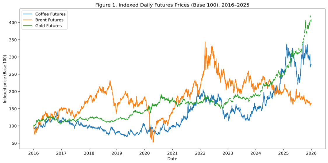
Figure 2.
Empirical distribution of daily logarithmic returns.
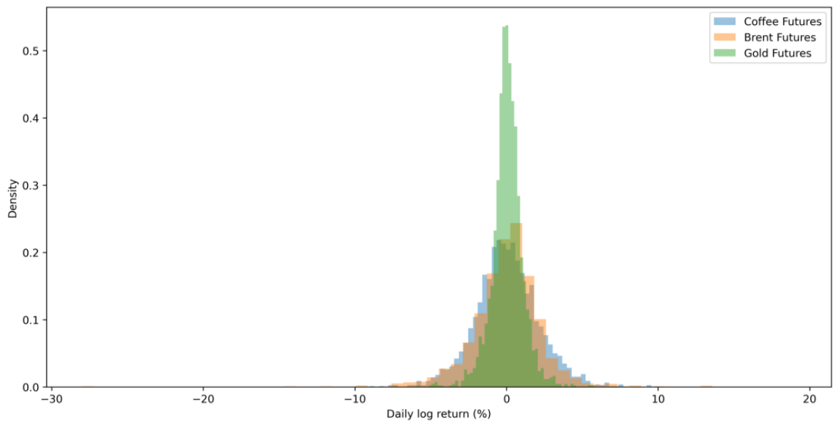
Figure 3.
Annualized rolling volatility of logarithmic returns.
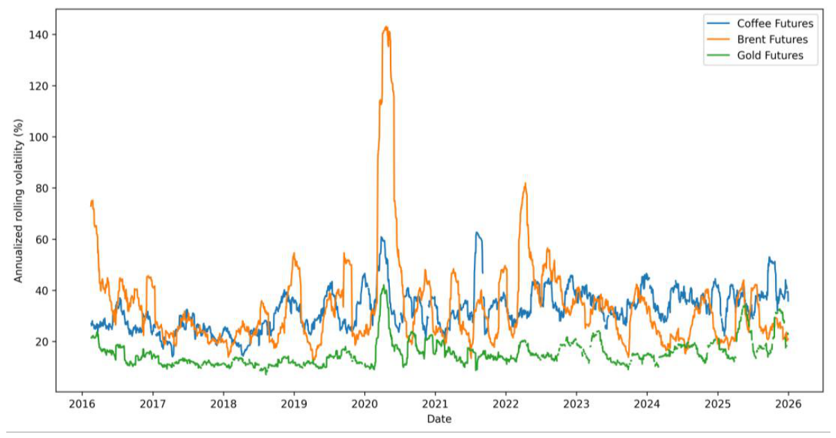
Figure 4.
Log-log scaling plots for long-memory estimation in commodity futures. (a) Coffee; (b) Brent; (c) Gold.
Figure 4.
Log-log scaling plots for long-memory estimation in commodity futures. (a) Coffee; (b) Brent; (c) Gold.
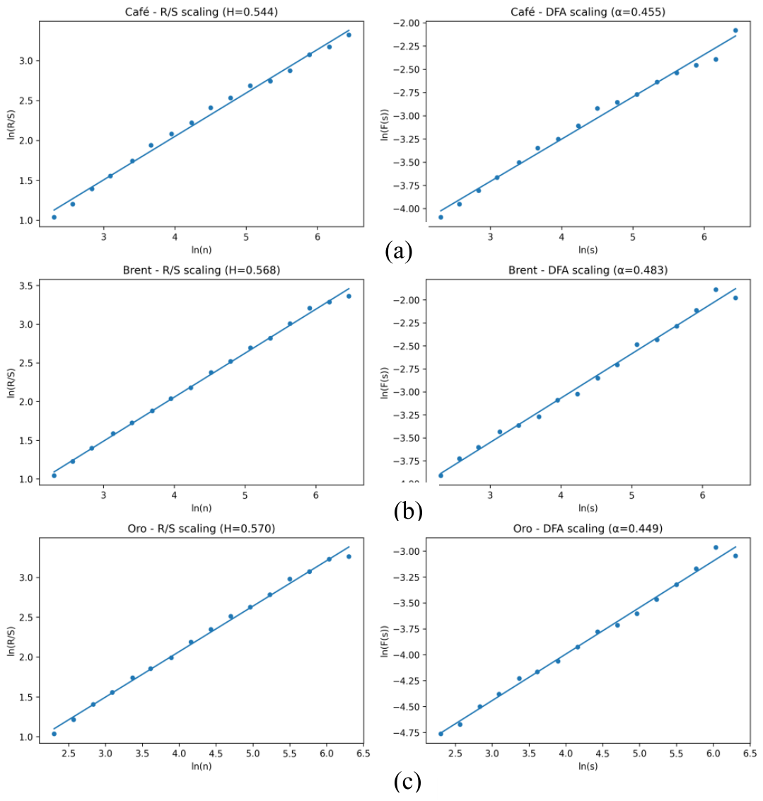
Figure 5.
Rolling Hurst coefficient.
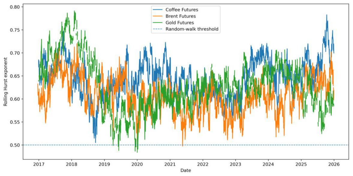
Figure 6.
Generalized Hurst exponents.
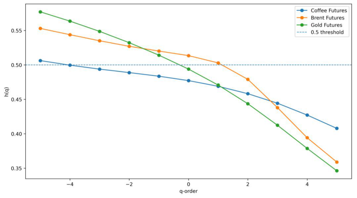
Figure 7.
Multifractal mass exponent
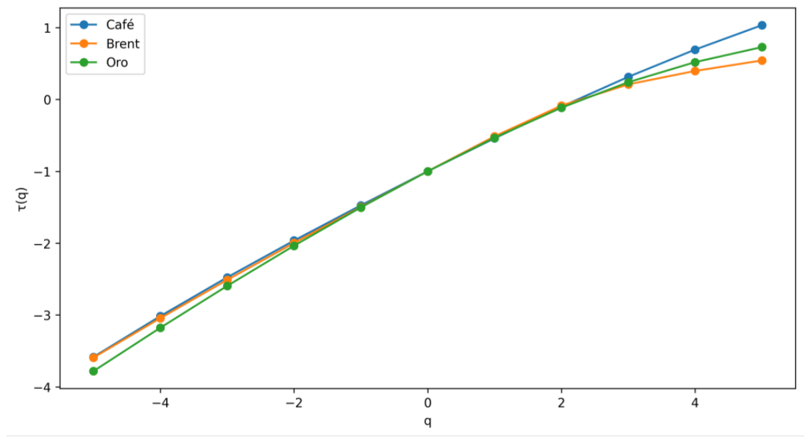
Figure 8.
Multifractal spectrum
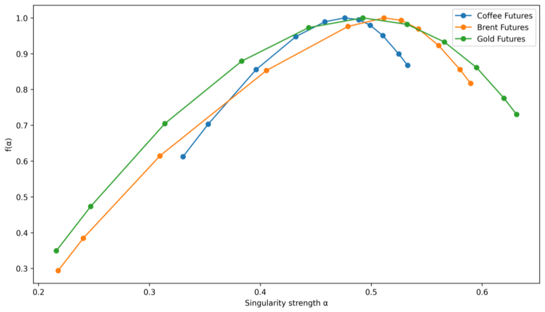
Figure 9.
ACF and PACF of logarithmic returns. (a) Coffee; (b) Brent; (c) Gold.
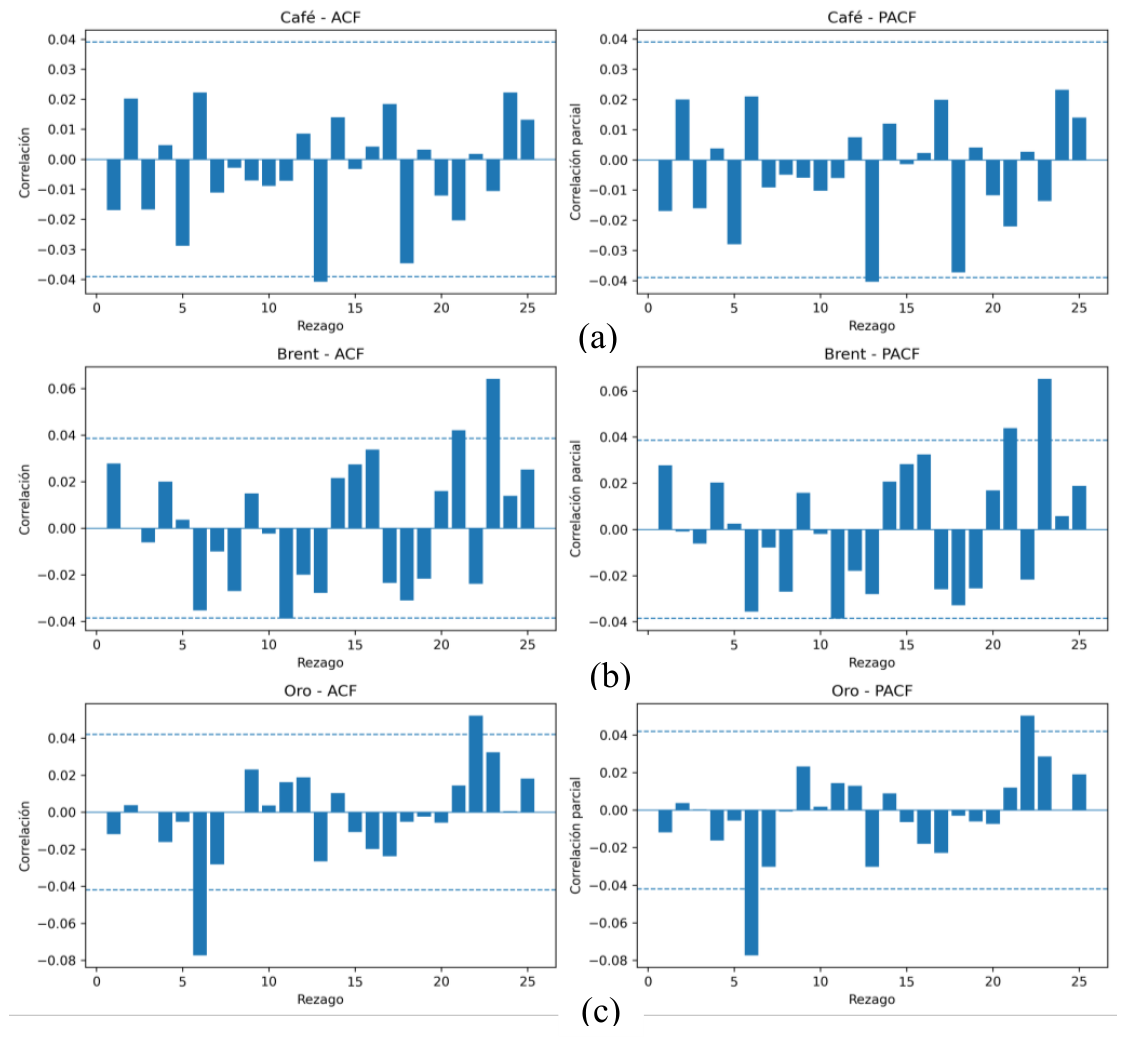
Figure 10.
ACF and PACF of squared returns. (a) Coffee; (b) Brent; (c) Gold.
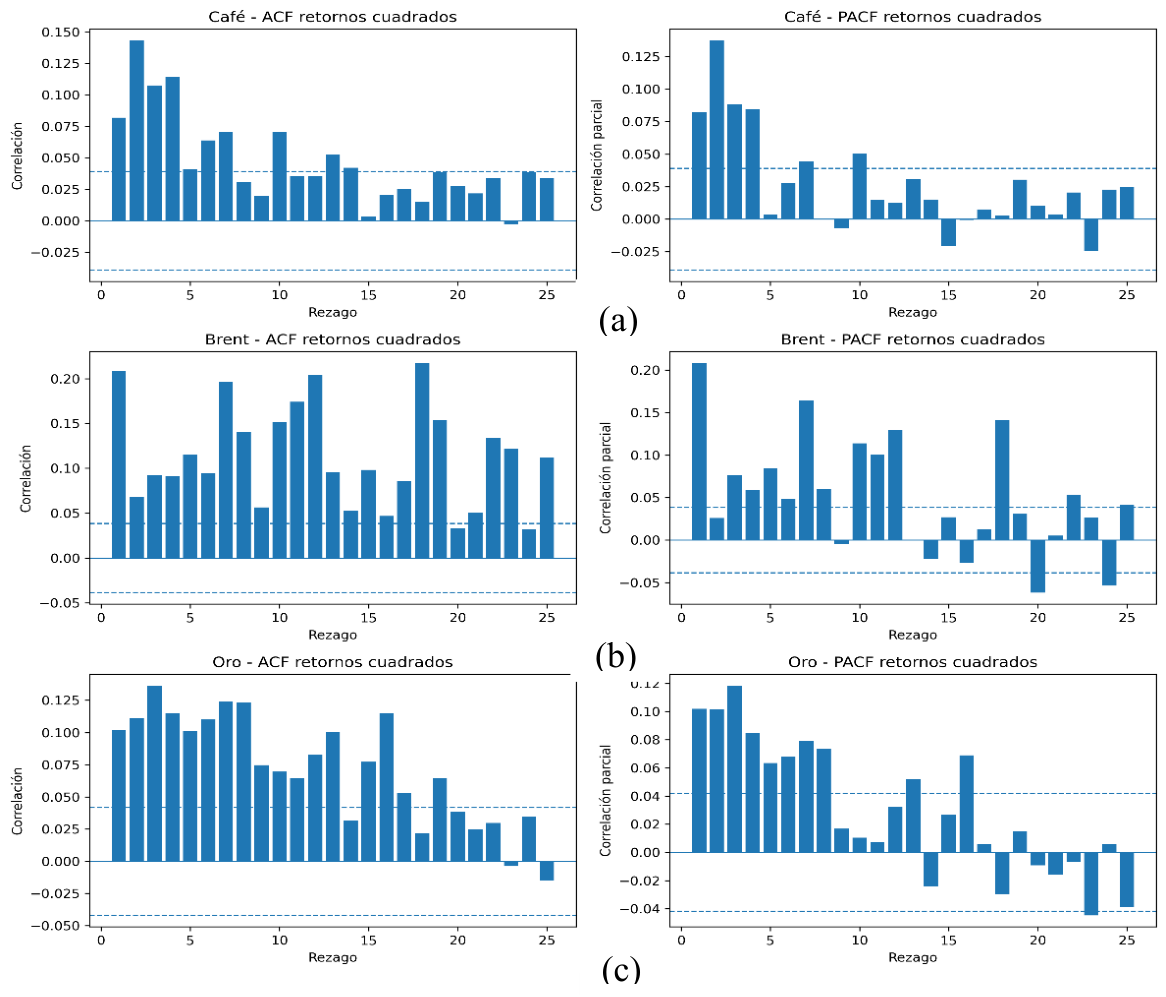
Figure 11.
Conditional volatility estimated with selected GARCH models.
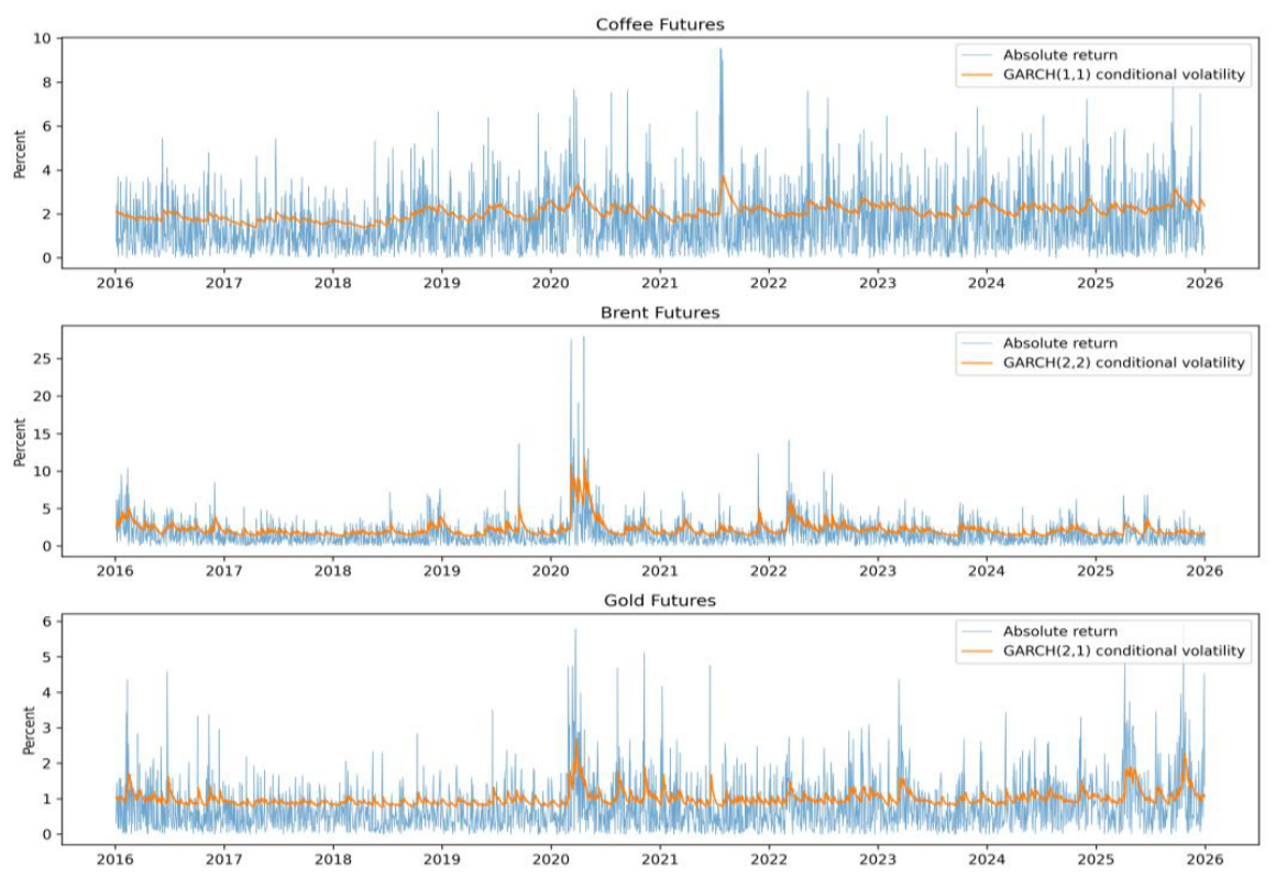
Figure 12.
Monte Carlo simulated trajectories for coffee, Brent and gold.
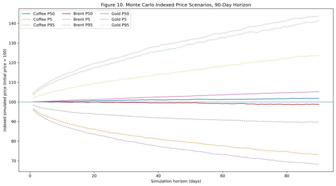
Figure 13.
Simulated terminal distribution at 90 days.
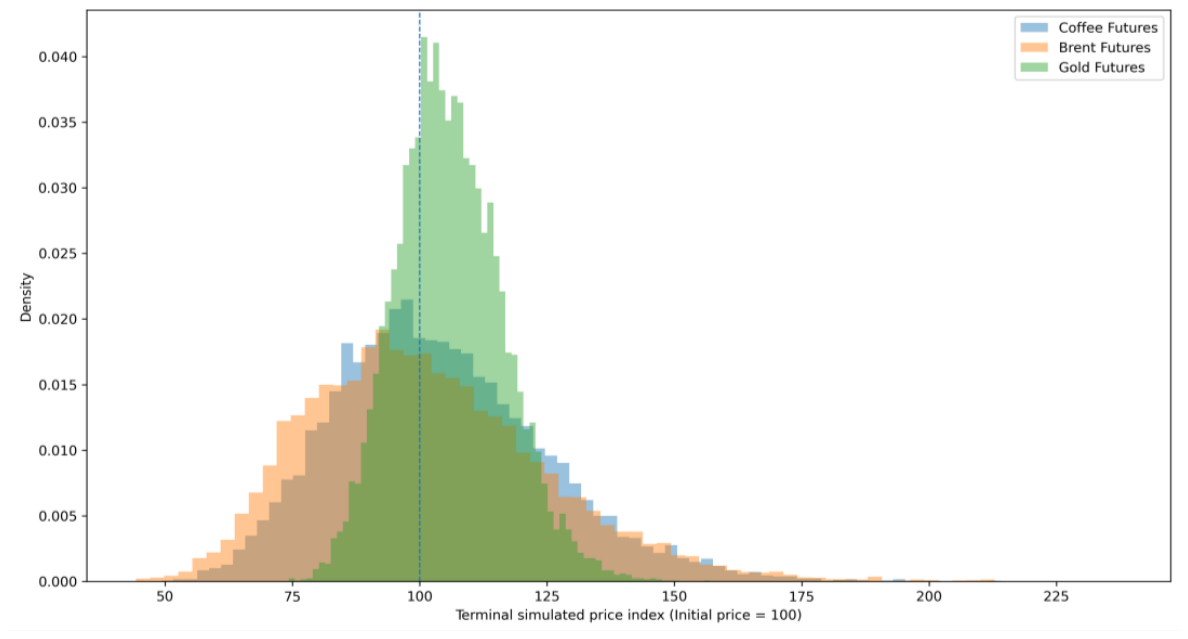
Figure 14.
Ex-post validation of Monte Carlo P5-P95 intervals.
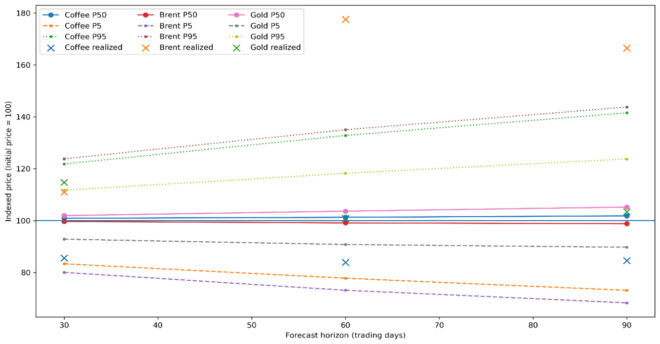
Figure 15.
Normal Q-Q plots of daily log returns.
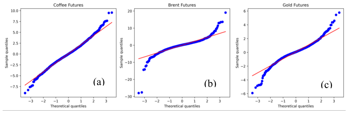
Figure 16.
Candidate ARIMA models according to the AIC criterion. (a) Coffee; (b) Brent; (c) Gold.
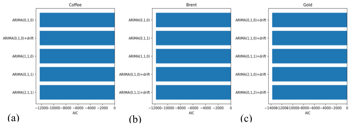
Figure 17.
Autocorrelation of residuals from the selected mean models.
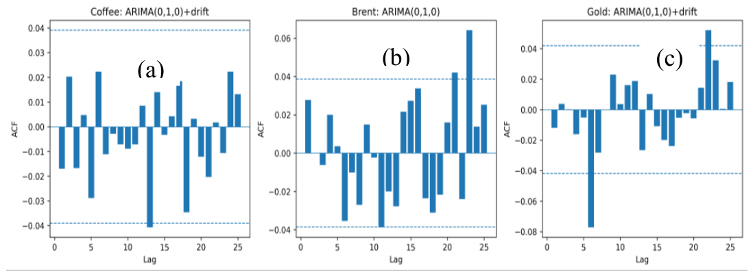
Figure 18.
Normalized location of observed 2026 prices within the simulated P5-P95 intervals.
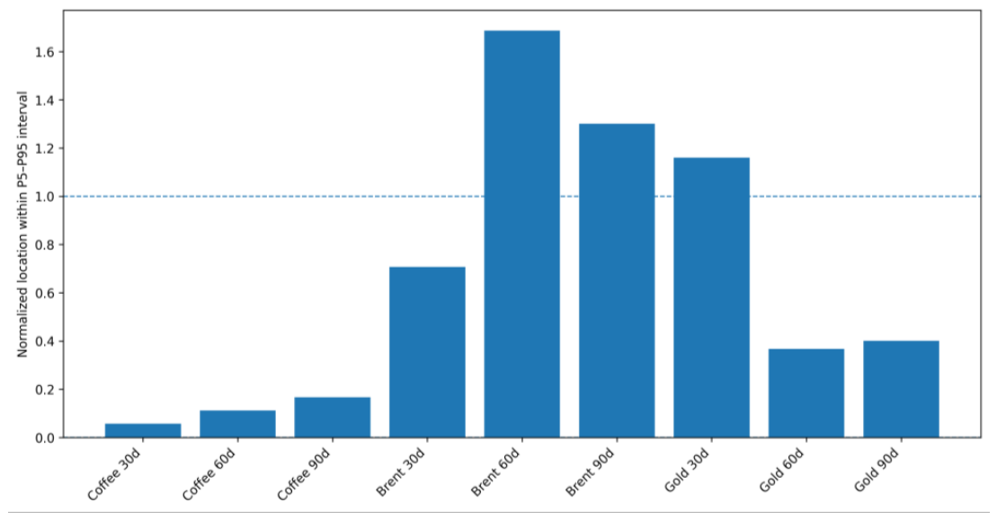

Table 1.
Phases of the methodological design applied in the study.
| Phase | Methodological component | Main techniques | Analytical purpose |
|---|---|---|---|
| 1 | Cleaning and organization | Ordering, validation and removal of inconsistent records | Ensure temporal consistency |
| 2 | Transformation and characterization | Logarithmic returns, descriptive statistics and rolling volatility | Identify distribution, dispersion and risk episodes |
| 3 | Memory diagnosis | Hurst R/S, DFA and rolling windows | Evaluate persistence, antipersistence or randomness |
| 4 | Multifractal analysis | MF-DFA, , τ(q) and | Determine heterogeneous scaling |
| 5 | Mean modeling | Random Walk, Drift, ARIMA and ARFIMA | Evaluate forecasting performance |
| 6 | Conditional volatility | ARCH LM, GARCH and FIGARCH-type | Compare variance persistence |
| 7 | Probabilistic scenarios | Monte Carlo and ex-post validation | Evaluate plausibility of P5-P95 intervals |
Table 2.
Description of the historical futures series used in the study.
| Commodity | Identification | Asset nature | Quotation unit | Observed period | Valid prices | Valid returns |
|---|---|---|---|---|---|---|
| Coffee Futures | Coffee | Agricultural commodity | U.S. cents per pound | 04/01/2016-31/12/2025 | 2515 | 2514 |
| Brent Futures | Brent | Energy commodity | U.S. dollars per barrel | 04/01/2016-31/12/2025 | 2581 | 2580 |
| Gold Futures (GC) | Gold | Precious metal / safe-haven asset | U.S. dollars per troy ounce | 04/01/2016-30/12/2025 | 2187 | 2186 |
Table 3.
Interpretation criteria for long-term memory.
| Exponent range | Statistical interpretation | Interpretation in futures markets | Methodological implication |
|---|---|---|---|
| H o < 0.5 | Antipersistence | Movements tend to revert | Models with reversal or low persistence |
| H o ≈ 0.5 | Random behavior | Series close to a random walk | Benchmark Random Walk |
| H o > 0.5 | Persistence | Movements tend to maintain direction | Contrast with ARFIMA/FIGARCH |
| H o >> 0.5 | High persistence | Potentially strong temporal dependence | Verify robustness and structural changes |
Table 4.
Empirical configuration of the MF-DFA analysis.
| Parameter | Applied value | Function |
|---|---|---|
| Series analyzed | Daily logarithmic returns | Avoid inference on nonstationary prices |
| q range | -5 to 5 | Capture small and large fluctuations |
| Scales s | Logarithmic windows between 16 and N/4 | Evaluate scaling across time windows |
| Polynomial order | 1 | Remove local linear trends |
| Multifractal criterion | Variation of , and | Determine scaling heterogeneity |
Table 5.
Descriptive statistics of daily logarithmic returns.
| Commodity | Observations | Daily mean | Median | Std. deviation | Minimum | Maximum | Skewness | Kurtosis |
| Coffee | 2514 | 0.046% | 0.000% | 2.102% | -9.021% | 9.557% | 0.0987 | 0.9801 |
| Brent | 2580 | 0.019% | 0.156% | 2.437% | -27.976% | 19.077% | -1.0929 | 17.7953 |
| Gold | 2186 | 0.064% | 0.058% | 1.034% | -5.913% | 5.775% | -0.1966 | 3.6620 |
Table 6.
Long-term memory estimates for the full sample.
| Commodity | Observations | Hurst R/S | DFA alpha | Joint interpretation |
|---|---|---|---|---|
| Coffee | 2514 | 0.537 | 0.460 | Weak R/S persistence, not confirmed by DFA |
| Brent | 2580 | 0.564 | 0.471 | Moderate R/S persistence, attenuated by DFA |
| Gold | 2186 | 0.560 | 0.448 | R/S persistence, DFA signal below 0.5 |
Table 7.
Long-term memory estimates by subperiod.
| Commodity | Subperiod | Hurst R/S | DFA alpha | Subperiod interpretation |
|---|---|---|---|---|
| Coffee | Pre-COVID | 0.586 | 0.464 | R/S persistence without DFA confirmation |
| Coffee | COVID | 0.621 | 0.476 | Stronger R/S signal, DFA close to randomness |
| Coffee | Recent regime | 0.642 | 0.547 | Partially confirmed persistence |
| Brent | Pre-COVID | 0.588 | 0.490 | Persistent R/S, nearly random DFA |
| Brent | COVID | 0.589 | 0.560 | Persistence confirmed during crisis |
| Brent | Recent regime | 0.580 | 0.403 | R/S persistence, DFA reversal |
| Gold | Pre-COVID | 0.633 | 0.532 | Moderate persistence |
| Gold | COVID | 0.597 | 0.415 | R/S persistence, DFA reversal |
| Gold | Recent regime | 0.607 | 0.416 | R/S persistence, DFA reversal |
Table 8.
Summary of multifractal parameters by commodity.
| Commodity | h(-5) | h(0) | h(5) | ||||
|---|---|---|---|---|---|---|---|
| Coffee | 0.517 | 0.466 | 0.407 | 0.110 | 0.340 | 0.568 | 0.228 |
| Brent | 0.519 | 0.494 | 0.308 | 0.210 | 0.146 | 0.550 | 0.404 |
| Gold | 0.556 | 0.486 | 0.346 | 0.211 | 0.209 | 0.604 | 0.394 |
Table 9.
Out-of-sample evaluation of one-step-ahead forecasting models.
| Commodity | Model | MAE | RMSE | MAPE | Theil U | Interpretation |
|---|---|---|---|---|---|---|
| Coffee | Random Walk | 1.000 | 1.000 | 1.000 | 1.000 | Benchmark |
| Coffee | Drift | 0.991 | 0.994 | 0.988 | 0.994 | Marginal improvement |
| Coffee | ARFIMA | 1.018 | 1.021 | 1.015 | 1.021 | No predictive gain |
| Brent | Random Walk | 1.000 | 1.000 | 1.000 | 1.000 | Benchmark |
| Brent | Drift | 1.004 | 1.006 | 1.003 | 1.006 | No improvement |
| Brent | ARFIMA | 1.026 | 1.030 | 1.022 | 1.030 | Below the benchmark |
| Gold | Random Walk | 1.000 | 1.000 | 1.000 | 1.000 | Benchmark |
| Gold | Drift | 0.993 | 0.995 | 0.991 | 0.995 | Marginal improvement |
| Gold | ARFIMA | 1.011 | 1.016 | 1.009 | 1.016 | No predictive gain |
Table 10.
Selected GARCH models and subsequent diagnostics.
| Commodity | Selected model | Persistence | AIC | BIC | ARCH LM post-GARCH p-value | Decision |
|---|---|---|---|---|---|---|
| Coffee | GARCH(1,1) | 0.9882 | 10764.63 | 10782.12 | 0.0164 | Partial residual persistence |
| Brent | GARCH(2,2) | 0.9413 | 11087.02 | 11116.30 | 0.8720 | Adequate |
| Gold | GARCH(2,1) | 0.9070 | 6146.56 | 6187.32 | 0.8686 | Adequate |
Table 11.
Calibration parameters of the Monte Carlo simulation.
| Commodity | Initial price | Average daily return | Daily volatility | Simulations | Horizons |
|---|---|---|---|---|---|
| Coffee | 348.75 | 0.0405% | 2.10% | 10,000 | 30, 60 and 90 days |
| Brent | 60.85 | 0.0190% | 2.44% | 10,000 | 30, 60 and 90 days |
| Gold | 4386.30 | 0.0643% | 1.03% | 10,000 | 30, 60 and 90 days |
Table 12.
Simulated percentiles of future prices by commodity and horizon.
| Commodity | Horizon | P5 pessimistic | P50 baseline | Mean | P95 optimistic | P5-P95 range | Loss probability |
|---|---|---|---|---|---|---|---|
| Coffee | 30 days | 290.654 | 351.901 | 353.768 | 424.866 | 134.212 | 46.92% |
| Coffee | 60 days | 271.155 | 353.108 | 357.980 | 463.164 | 192.008 | 46.99% |
| Coffee | 90 days | 254.955 | 355.013 | 362.416 | 493.597 | 238.642 | 46.70% |
| Brent | 30 days | 48.677 | 60.649 | 61.177 | 75.324 | 26.647 | 50.98% |
| Brent | 60 days | 44.499 | 60.308 | 61.444 | 82.149 | 37.650 | 51.74% |
| Brent | 90 days | 41.541 | 60.113 | 61.698 | 87.465 | 45.924 | 51.92% |
| Gold | 30 days | 4071.657 | 4469.182 | 4474.258 | 4898.625 | 826.968 | 36.62% |
| Gold | 60 days | 3981.999 | 4543.944 | 4560.609 | 5185.028 | 1203.028 | 32.17% |
| Gold | 90 days | 3935.318 | 4613.926 | 4644.341 | 5427.711 | 1492.394 | 29.68% |
Table 13.
Ex-post validation of Monte Carlo scenarios with observed 2026 prices.
| Commodity | Horizon | Actual 2026 price | P5 | P50 | P95 | Validation | Normalized location |
|---|---|---|---|---|---|---|---|
| Coffee | 30 days | 298.30 | 290.65 | 351.90 | 424.87 | Within P5-P95 | 0.057 |
| Coffee | 60 days | 292.55 | 271.16 | 353.11 | 463.16 | Within P5-P95 | 0.111 |
| Coffee | 90 days | 294.80 | 254.95 | 355.01 | 493.60 | Within P5-P95 | 0.167 |
| Brent | 30 days | 67.52 | 48.68 | 60.65 | 75.32 | Within P5-P95 | 0.707 |
| Brent | 60 days | 108.01 | 44.50 | 60.31 | 82.15 | Outside P5-P95 | 1.687 |
| Brent | 90 days | 101.29 | 41.54 | 60.11 | 87.46 | Outside P5-P95 | 1.301 |
| Gold | 30 days | 5031.00 | 4071.66 | 4469.18 | 4898.62 | Outside P5-P95 | 1.160 |
| Gold | 60 days | 4423.60 | 3982.00 | 4543.94 | 5185.03 | Within P5-P95 | 0.367 |
| Gold | 90 days | 4533.30 | 3935.32 | 4613.93 | 5427.71 | Within P5-P95 | 0.401 |
Table 14.
Coverage of Monte Carlo intervals in the ex-post validation.
| Commodity | Evaluated horizons | Within P5-P95 | Outside P5-P95 | Coverage |
|---|---|---|---|---|
| Coffee | 3 | 3 | 0 | 100.0% |
| Brent | 3 | 1 | 2 | 33.3% |
| Gold | 3 | 2 | 1 | 66.7% |
| Total | 9 | 6 | 3 | 66.7% |
Disclaimer/Publisher’s Note: The statements, opinions and data contained in all publications are solely those of the individual author(s) and contributor(s) and not of MDPI and/or the editor(s). MDPI and/or the editor(s) disclaim responsibility for any injury to people or property resulting from any ideas, methods, instructions or products referred to in the content. |
© 2026 by the authors. Licensee MDPI, Basel, Switzerland. This article is an open access article distributed under the terms and conditions of the Creative Commons Attribution (CC BY) license (http://creativecommons.org/licenses/by/4.0/).
Copyright: This open access article is published under a Creative Commons CC BY 4.0 license, which permit the free download, distribution, and reuse, provided that the author and preprint are cited in any reuse.


