Trust as a Trajectory Property: An Epistemic Dynamics Framework for AI Evaluation

1. Introduction

Modern AI systems are increasingly embedded in evaluation pipelines that combine model predictions, LLM-based judges, human oversight, and recursive verification layers. In clinical decision support, a model emits a recommendation, a clinician either trusts or overrides it, and a downstream auditor may review the override [1,2]. In LLM evaluation, a base model produces a candidate answer, a judge model scores it, and a meta-judge may adjudicate disagreements. Each of these settings is studied today under a different vocabulary: calibration, agreement, override rate, ensemble diversity, judge bias. What is missing is a unified representation under which trust emerges from the structured evolution of the pipeline rather than from any single model’s output. A prior series of works developed the conceptual foundations for this shift—from verification as the real cost of AI [3], through epistemic frontiers and technology discontinuities [4], collective multi-agent epistemics [5], and trust budgets for the optimal control of scientific discovery [6]—but stopped short of a unified dynamical-systems formalization.

Existing evaluation theory treats trust implicitly as a property of a model at a point in time. Calibration research assumes that a well-calibrated confidence score is sufficient for downstream decision-making [7,8,9]; clinical implementations of this idea have been developed for diagnostic transparency [1] and risk prediction [10]. LLM-as-a-judge work treats agreement among judges as a proxy for evaluation quality [11,12]. Ensemble methods characterize diversity as a property of a fixed model collection [13,14]. Governance frameworks for clinical AI have been proposed [15,16] and broadly reviewed [2,17], but without a dynamical model of trust trajectories. None of these accounts for the temporal, recursive, and governance-bound structure of real evaluation pipelines.

• Gap.

There is no formal framework that (i) places models, judges, and human reviewers in a shared state space, (ii) defines operators that govern pipeline transitions, and (iii) characterizes pipeline failures as geometric regions rather than point-wise metrics. As a consequence, two systems with identical accuracy can exhibit vastly different trust behavior over time, and existing metrics cannot distinguish them.

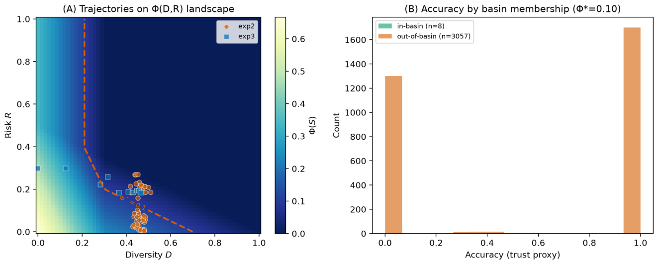
Figure 1. Empirical trajectories overlaid on the stability landscape estimated from MIMIC-IV data ($n=3,000$) and simulated multi-model experiments. (A) Trajectories in the diversity–risk plane; the dashed contour marks the stability zone boundary (${\Phi }^{*}=0.10$). In-basin points (green) cluster at low risk and high accuracy; out-of-basin points (red) span the full range. (B) Trust (accuracy proxy) histograms by stability zone membership. In-basin trajectories achieve $80.3\%$ accuracy versus $56.4\%$ for out-of-basin. This figure previews the paper’s central empirical finding: stability zone membership predicts trust outcomes. The framework that defines these zones is developed in the following sections. (A companion analysis using real clinician trust from MIMIC override logs yields $d=0.70$, Section 8.)

Figure 1. Empirical trajectories overlaid on the stability landscape estimated from MIMIC-IV data ($n=3,000$) and simulated multi-model experiments. (A) Trajectories in the diversity–risk plane; the dashed contour marks the stability zone boundary (${\Phi }^{*}=0.10$). In-basin points (green) cluster at low risk and high accuracy; out-of-basin points (red) span the full range. (B) Trust (accuracy proxy) histograms by stability zone membership. In-basin trajectories achieve $80.3\%$ accuracy versus $56.4\%$ for out-of-basin. This figure previews the paper’s central empirical finding: stability zone membership predicts trust outcomes. The framework that defines these zones is developed in the following sections. (A companion analysis using real clinician trust from MIMIC override logs yields $d=0.70$, Section 8.)

• Contribution.

We address this gap with a dynamical-systems formulation of AI evaluation. Our contributions are:

• We define an epistemic state space $\mathbb{E}$ that uniformly represents AI systems, evaluators, and hybrid workflows (Section 3).
• We introduce an operator algebra that separates a prediction generator $\mathcal{P}$, three state transformations $\{\mathcal{J},\mathcal{V},\mathcal{G}\}$, and an aggregation operator $\mathcal{A}$ over evaluator ensembles. The transformations are composable: any finite sequence yields a well-defined trajectory (Section 4).
• We develop a stability theory that decouples admissibility (one axiom) from stability-defining conditions (five), defines collapse as the violation of any condition, and introduces a stability indicator $\Phi$ whose sub-level sets define stability zones (Section 5).
• We operationalize all eight state variables as estimators computable from logs, model outputs, and human feedback (Section 6).
• We instantiate four experiments on MIMIC-IV override logs, multi-model LLM judges, and recursive verification pipelines—using both simulation and real LLMs (Ollama: Llama 3.1, Phi 4, Qwen 2.5)—validating all five trajectory-level claims, including the central thesis that stability zone membership predicts trust ($d=0.70$ on $n=3,000$ ICU stays) (Section 7 and Section 8).

The central thesis is summarized in one sentence:

Trustworthy AI systems are those whose epistemic trajectories remain within a bounded stability basin under recursive evaluation and bounded verification cost.

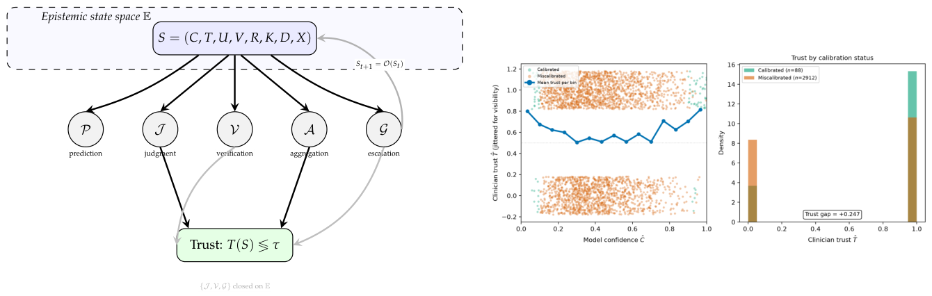
Figure 2. (Left) Epistemic state space ontology. A system occupies a state $S=(C,T,U,V,R,K,D,X)$. Operators $\mathcal{P}$ (prediction), $\mathcal{J}$ (judgment), $\mathcal{V}$ (verification), $\mathcal{A}$ (aggregation), $\mathcal{G}$ (escalation) govern transitions, forming trajectories $\mathcal{T}=(S_0,\dots ,S_t)$. Transformations $\{\mathcal{J},\mathcal{V},\mathcal{G}\}$ are closed under composition on $\mathbb{E}$. Trust decisions occur at boundary $\tau$, driven most directly by judgment and aggregation.(Right) The state space instantiated from MIMIC-IV data ($n=3,000$). Confidence $\widehat{C}$ vs clinician trust $\widehat{T}$ (jittered). Green: calibrated; red: miscalibrated. Blue line: mean trust per bin. Trust gap: $+0.167$ (H1).

Figure 2. (Left) Epistemic state space ontology. A system occupies a state $S=(C,T,U,V,R,K,D,X)$. Operators $\mathcal{P}$ (prediction), $\mathcal{J}$ (judgment), $\mathcal{V}$ (verification), $\mathcal{A}$ (aggregation), $\mathcal{G}$ (escalation) govern transitions, forming trajectories $\mathcal{T}=(S_0,\dots ,S_t)$. Transformations $\{\mathcal{J},\mathcal{V},\mathcal{G}\}$ are closed under composition on $\mathbb{E}$. Trust decisions occur at boundary $\tau$, driven most directly by judgment and aggregation.(Right) The state space instantiated from MIMIC-IV data ($n=3,000$). Confidence $\widehat{C}$ vs clinician trust $\widehat{T}$ (jittered). Green: calibrated; red: miscalibrated. Blue line: mean trust per bin. Trust gap: $+0.167$ (H1).

2. Related Work

• Confidence calibration.

Guo et al. [7] introduced temperature scaling for modern neural networks, and Naeini et al. [8] established reliability diagrams and the expected calibration error as standard diagnostics. Kumar et al. [9] introduced distribution-free calibration guarantees. These works treat calibration as a property of a model’s output distribution; they do not model the downstream pipeline that consumes the calibrated score.

• LLM-as-a-judge.

Zheng et al. [11] formalized LLM-based evaluation and quantified judge–judge agreement. Wang et al. [12] demonstrated systematic biases in LLM judges, including position and length bias. These works study judges as isolated evaluators rather than as operators in a recursive pipeline.

• Verbalized and epistemic uncertainty in LLMs.

Kadavath et al. [18] showed that language models can express calibrated uncertainty verbally. Kuhn et al. [19] introduced semantic uncertainty estimates based on linguistic invariances, and Lin et al. [20] trained models to express knowledge uncertainty in words. The present framework treats such signals as observable proxies for one coordinate (C) of a richer state.

• Ensembling and diversity.

Krogh and Vedelsby [13] established that ensemble diversity reduces error, formalized as ambiguity decomposition. Wang et al. [14] applied this to chain-of-thought reasoning. Cobbe et al. [21] trained verifiers for mathematical reasoning, introducing recursive verification. We recast these results as instances of operator composition over a shared state space.

• Clinical decision support.

Johnson et al. [22] provides the MIMIC-IV dataset that anchors our first experiment. Override behavior in clinical AI is the empirical access point for trust trajectories.

• Dynamical systems background.

The trajectory formulation draws on discrete-time dynamical systems theory [23] and Lyapunov stability [24], though we do not assume continuous-time dynamics or require equilibrium convergence.

• Collective intelligence and diversity.

The diversity–risk coupling (Condition 3) is related to the Diversity Prediction Theorem [25], which decomposes collective error into individual accuracy and diversity. Our formulation extends this from static crowds to temporal verification pipelines.

• Social epistemology.

The epistemic state space embeds concepts from social epistemology [26], particularly the role of diverse perspectives in knowledge validation. Collapse modes (C) and (D) instantiate the failure of epistemic diversity under recursive evaluation.

• Prior work in this program.

The present paper unifies a series of conceptual and empirical contributions by the author. The Computational Epistemics series [3,4,5,6] established verification as the dominant cost of AI-driven discovery and formalized collective computational epistemics in multi-agent networks. On the empirical side, Yu et al. [1] introduced a dynamic framework for confidence calibration and transparency in clinical AI diagnostics; the escalation operator generalizes the selective-prediction (reject-option) literature [27,28]. The current paper integrates these strands into a single dynamical-systems formulation.

3. Epistemic State Space

We define the ontology over which all subsequent dynamics are constructed. The eight-variable state space formalizes and extends the conceptual model introduced across the computational epistemics program [3] and builds on established frameworks for epistemic uncertainty decomposition [29].

 Definition 1

(Epistemic state space). The epistemic state space is the product space

$$\mathbb{E}={[0,1]}^6\times {\mathbb{R}}_{\ge 0}^2.$$

An epistemic state is an 8-tuple

$$S=(C,T,U,V,R,K,D,X)\in \mathbb{E},$$

with the following coordinates:

• $C\in [0,1]$ — system confidence in its current claim;
• $T\in [0,1]$ — degree of trust extended by the downstream consumer;
• $U\in [0,1]$ — normalized epistemic uncertainty;
• $V\in {\mathbb{R}}_{\ge 0}$ — cumulative verification effort;
• $R\in [0,1]$ — normalized epistemic risk;
• $K\in {\mathbb{R}}_{\ge 0}$ — cumulative cost;
• $D\in [0,1]$ — epistemic diversity across evaluators;
• $X\in [0,1]$ — transparency of the current claim.

The partition into $[0,1]$ and ${\mathbb{R}}_{\ge 0}$ coordinates reflects that V and K are cumulative quantities that grow along a trajectory, while the remaining six are per-state intensities bounded per decision.

 Definition 2

(Accuracy functional). The accuracy functional $a:\mathbb{E}\to [0,1]$ maps a state to the empirical correctness probability of the underlying claim, measured against ground truth whenever available and estimated by an independent gold-standard evaluator otherwise.

3.1. Admissibility

We require only one axiom of every trajectory. It states a basic well-formedness property (cost is monotone) and defines the universe of pipelines the framework can describe.

 Axiom 1

(Cost accumulation). Along any trajectory, cost is non-decreasing: $K_{t+1}\ge K_t$ for all t.

Axiom 1 is the only universal admissibility requirement. Trajectories that violate it (e.g., pipelines that fabricate negative cost) fall outside the framework’s scope.

3.2. Stability Conditions

The following five conditions are not assumed; they define stability. A trajectory may satisfy any subset of them, and the subset it violates identifies its collapse mode (Definition 11). Each condition is stated in the discrete form appropriate to the operator algebra of Section 4.

 Condition 1

(Calibration). For tolerance $\delta \ge 0$, $|C_t-a\left(S_t\right)|\le \delta$ for all t.

 Condition 2

(Risk–uncertainty coupling). For any two states $S,S^{\prime }\in \mathbb{E}$ differing only in the U coordinate, $U>U^{\prime }\Rightarrow R\ge R^{\prime }$. This is a cross-sectional property of the state space (higher-uncertainty states have weakly higher risk), not a trajectory implication; it is compatible with operators such as $\mathcal{V}$ that reduce R at fixed U.

 Condition 3

(Diversity–risk coupling). There exist $\beta ,R_0>0$ such that $R_t\ge R_0(1-D_t)$ for all t. The bound is trivial at $D_t=1$ and forces $R_t\ge R_0$ when diversity is fully depleted.

 Condition 4

(Verification efficacy). Whenever $\mathcal{V}$ is applied between t and $t+1$, $R_{t+1}\le R_t$.

 Condition 5

(Marginal verification cost). There exists $c_{min}>0$ such that $K_{t+1}-K_t\ge c_{min}·(V_{t+1}-V_t)$ whenever $\mathcal{V}$ or $\mathcal{G}$ is applied.

Conditions 1–5 define the five axes along which a trajectory can fail. Crucially, they are independent: a trajectory may be calibrated (Condition 1) while failing diversity (Condition 3), as in a single-model judge with accurate confidence but no evaluator disagreement. Section 5 formalizes how the conjunction of these conditions defines the stable basin and how each individual violation defines a named collapse mode.

4. Epistemic Dynamics

State transitions are governed by an operator algebra with three distinguishable roles: a generator that initializes a state from an external input, transformations that evolve a single state into its successor, and an aggregator that combines several evaluator states into one. The transformation set $\{\mathcal{J},\mathcal{V},\mathcal{G}\}$ is composable: any finite sequence of transformations applied to an initial state yields a well-defined trajectory (Proposition 1).

4.1. Operators

Let $\mathcal{X}$ denote the input space (e.g., patient features, prompts).

Generator.

 Definition 3

(Prediction generator). $\mathcal{P}:\mathcal{X}\to \mathbb{E}$ maps an input $x\in \mathcal{X}$ to an initial state $S_0=\mathcal{P}\left(x\right)$ with $V_0=K_0=0$ and $(C_0,T_0,U_0,R_0,D_0,X_0)$ determined by the model’s output distribution.

$\mathcal{P}$ is not in the operator algebra proper; it constructs $S_0$ and is then composed away.

Transformations ($\mathbb{E}\to \mathbb{E}$).

 Definition 4

(Judgment operator). $\mathcal{J}:\mathbb{E}\to \mathbb{E}$ produces an evaluation of the current claim. It writes $(C,X,U)\leftarrow ({\mathcal{J}}_C,{\mathcal{J}}_X,{\mathcal{J}}_U)$ and preserves $(V,K,R,D)$. The preservation of R encodes that judging alone neither verifies nor mitigates risk.

 Definition 5

(Verification operator). $\mathcal{V}:\mathbb{E}\to \mathbb{E}$ performs an external check. It increments $(V,K)\leftarrow (V+\Delta V,K+\Delta K)$ with $\Delta V,\Delta K>0$, decrements $R\leftarrow R-\Delta R$ for some $\Delta R\ge 0$, and preserves $(C,T,U,D,X)$.

 Definition 6

(Escalation operator). $\mathcal{G}:\mathbb{E}\to \mathbb{E}$ triggers a higher-order review. It increments $(V,K)\leftarrow (V+\Delta V_{\mathrm{esc}},K+\Delta K_{\mathrm{esc}})$ with $\Delta K_{\mathrm{esc}}\ge \Delta K$ for any single $\mathcal{V}$ application, may update $(C,R)$, and preserves $(T,U,D,X)$. The escalation operator formalizes the selective-prediction (reject-option) mechanism studied in Geifman and El-Yaniv [27] and extended to human-AI collaboration by Mozannar and Sontag [28].

Aggregator (over evaluator ensembles).

 Definition 7

(Ensemble). An ensemble of size n at time t is a collection ${\Sigma }_t=(S_t^{\left(1\right)},\dots ,S_t^{\left(n\right)})\in {\mathbb{E}}^n$ of evaluator states produced by n parallel transformations applied to a common predecessor state.

 Definition 8

(Aggregation operator). $\mathcal{A}:{\mathbb{E}}^n\to \mathbb{E}$ maps an ensemble ${\Sigma }_t$ to a single consensus state $S_{t+1}=\mathcal{A}\left({\Sigma }_t\right)$. The diversity coordinate of $S_{t+1}$ is

$$D_{t+1}=1-{\displaystyle \frac{2}{n(n-1)}}\sum _{i<j}\mathrm{sim}\left(S_t^{\left(i\right)},S_t^{\left(j\right)}\right),$$

where $\mathrm{sim}:\mathbb{E}\times \mathbb{E}\to [0,1]$ is a domain-appropriate state similarity. The remaining coordinates of $S_{t+1}$ are obtained by an aggregation rule (e.g., weighted mean of $(C,R,U,X)$; sum of $(V,K)$).

The ensemble structure of Definition 7 is the natural locus for collapse mode (C) (Section 5): the inter-evaluator variance ${\mathrm{Var}}_i\left(S_t^{\left(i\right)}\right)$ is well-defined on ${\Sigma }_t$.

4.2. Trajectories

 Definition 9

(Epistemic trajectory). An epistemic trajectory of horizon T is a sequence $\mathcal{T}=(S_0,S_1,\dots ,S_T)$ with $S_0=\mathcal{P}\left(x_0\right)$ and

$$S_{t+1}={\mathcal{O}}_t(S_t;x_t,{\xi }_t),{\mathcal{O}}_t\in \{\mathcal{J},\mathcal{V},\mathcal{G}\},$$

where ${\xi }_t$ captures sampling and human-behavior stochasticity. Ensemble sub-trajectories are admitted at any t by replacing the single transition $S_t\mapsto S_{t+1}$ with a two-step transition

$$S_t\mapsto {\Sigma }_t=({\mathcal{J}}^{\left(1\right)}\left(S_t\right),\dots ,{\mathcal{J}}^{\left(n\right)}\left(S_t\right))\mapsto S_{t+1}=\mathcal{A}\left({\Sigma }_t\right),$$

i.e., parallel judgment by n evaluators followed by aggregation. The ensemble ${\Sigma }_t$ is observable at time t and supports measurement of inter-evaluator variance.

The canonical evaluation pipeline is now expressible as a composition of $\mathbb{E}\to \mathbb{E}$ transformations, optionally punctuated by an ensemble step:

$$\mathcal{T}=\left(\mathcal{P}\left(x_0\right),\mathcal{J}\circ \mathcal{P}\left(x_0\right),\mathcal{V}\circ \mathcal{J}\circ \mathcal{P}\left(x_0\right),\mathcal{G}\circ \mathcal{V}\circ \mathcal{J}\circ \mathcal{P}\left(x_0\right)\right),$$

or, with an ensemble at the second step,

$$\mathcal{T}=\left(\mathcal{P}\left(x_0\right),\mathcal{A}\circ \Sigma [{\mathcal{J}}^{\left(1\right)},\dots ,{\mathcal{J}}^{\left(n\right)}]\circ \mathcal{P}\left(x_0\right),\mathcal{V}\circ \dots \right).$$

 Proposition 1

(Composability of the transformation set). The transformation set $\{\mathcal{J},\mathcal{V},\mathcal{G}\}$ is composable: any finite composition of transformations applied to an initial state $S_0\in \mathbb{E}$ yields a well-defined trajectory in $\mathbb{E}$.

Proof. 

Each transformation maps $\mathbb{E}\to \mathbb{E}$ by Definitions 4–6. The composition of measurable maps $\mathbb{E}\to \mathbb{E}$ is a measurable map $\mathbb{E}\to \mathbb{E}$. Application to $S_0\in \mathbb{E}$ therefore yields a well-defined state at every finite horizon. The aggregator $\mathcal{A}$ has signature ${\mathbb{E}}^n\to \mathbb{E}$ and is admitted only at ensemble sub-steps where an ${\mathbb{E}}^n$-valued ${\Sigma }_t$ has been constructed by parallel transformations; it is not part of the $\mathbb{E}\to \mathbb{E}$ closure claim.    □

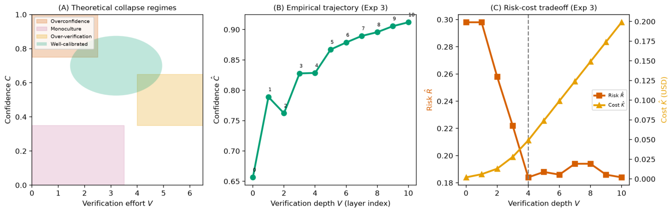
Figure 3. Empirical epistemic trajectory from the recursive verification experiment (Experiment 3, simulated graduated pipeline, 500 items). (A) Theoretical collapse regimes in the verification–confidence plane: well-calibrated region (green), overconfidence (red), monoculture (magenta), and over-verification (orange). (B) Empirical trajectory: confidence $\widehat{C}$ improves through depth 3, then saturates. (C) Risk–cost tradeoff: error rate $\widehat{R}$ decreases through depth 3 while cost $\widehat{K}$ grows linearly; optimal depth $n^{*}=4$ occurs at the benefit–cost crossover. Compare panel (A)’s theoretical regimes with the empirically observed path in (B)–(C): the trajectory traverses multiple regimes before settling in the well-calibrated region at moderate verification depth.

Figure 3. Empirical epistemic trajectory from the recursive verification experiment (Experiment 3, simulated graduated pipeline, 500 items). (A) Theoretical collapse regimes in the verification–confidence plane: well-calibrated region (green), overconfidence (red), monoculture (magenta), and over-verification (orange). (B) Empirical trajectory: confidence $\widehat{C}$ improves through depth 3, then saturates. (C) Risk–cost tradeoff: error rate $\widehat{R}$ decreases through depth 3 while cost $\widehat{K}$ grows linearly; optimal depth $n^{*}=4$ occurs at the benefit–cost crossover. Compare panel (A)’s theoretical regimes with the empirically observed path in (B)–(C): the trajectory traverses multiple regimes before settling in the well-calibrated region at moderate verification depth.

5. Stability Theory

This section identifies the conditions under which a trajectory is stable and describes the collapse regimes that emerge when those conditions fail.

5.1. Stable Trajectories

 Definition 10

($(ϵ,\delta ,D_{min})$-stability). Given constants $ϵ,\delta ,D_{min}>0$, a trajectory $\mathcal{T}$ is$(ϵ,\delta ,D_{min})$-stable if at every $t\in \{0,\dots ,T-1\}$ all of the following hold jointly:

(i)

$|R_{t+1}-R_t|\le ϵ$        (bounded risk drift),

(ii)

Condition 1 holds with tolerance δ,

(iii)

$D_t\ge D_{min}$      (non-degenerate diversity),

(iv)

Conditions 2 and 4 hold,

(v)

Condition 5 holds with $c_{min}$.

Definition 10 is non-vacuous: a generic admissible trajectory (satisfying only Axiom 1) need not satisfy any of (i)–(v), since the transformation operators are not constrained a priori to preserve them. Stability is therefore a property of operator behavior, not of the axiom system.

5.2. Collapse Regimes

Collapse modes (A) and (B) are direct falsifications of Conditions 1 and 4 respectively. Collapse modes (C) and (D) are threshold-crossing events: they occur when a coordinate exceeds a critical value even though no condition is formally violated. All four are detectable by the empirical tests of Section 6.

 Definition 11

(Epistemic collapse). A trajectory $\mathcal{T}$collapsesat time τ if at least one of the following holds:

(A) 

Overconfidence collapse (Condition 1 violation). $C_{\tau }-a\left(S_{\tau }\right)>\delta$. The system is more confident than its accuracy warrants. The symmetric case $a\left(S_{\tau }\right)-C_{\tau }>\delta$ (underconfidence) also violates Condition 1 but is not a named collapse mode because it produces over-conservative behavior rather than unsafe trust; we note the asymmetry and restrict attention to the overconfidence direction.

(B) 

Verification breakdown (Condition 4 violation). A $\mathcal{V}$ step occurs at τ with $R_{\tau }>R_{\tau -1}$: verification was applied but risk increased.

(C) 

Monoculture collapse (diversity threshold). $D_{\tau }<D_{min}$ and, for the ensemble ${\Sigma }_{\tau }$ admitted by Definition 7, ${\mathrm{Var}}_i\left(S_{\tau }^{\left(i\right)}\right)\to 0$ while $R_{\tau }\ge R_0$. Diversity is depleted and evaluators agree on errors. Note: Condition 3 remains formally satisfied (it forces $R\ge R_0$ at low D); the collapse is the consequence of depleted diversity, not the violation of the bound.

(D) 

Over-verification divergence (cost–risk threshold). $K_{\tau }-K_{\tau -1}>\kappa$ while $|R_{\tau }-R_{\tau -1}|<\eta$ for fixed $\kappa ,\eta >0$: cost grows without proportional risk reduction. Condition 5 remains satisfied; the collapse is the crossing of a cost-efficiency threshold.

Modes (A) and (B) co-occur when a miscalibrated verifier both overtrusts and amplifies risk. Modes (C) and (D) represent opposite failure extremes: insufficient diversity drives (C), while excessive verification drives (D).

5.3. Stability Indicator

States can be compared by how close they are to satisfying Conditions 1 and 3. We define a heuristic indicator that aggregates the per-condition penalties; it is one of several possible scalar summaries and should be interpreted as a diagnostic tool rather than a universal measure.

 Definition 12

(Stability indicator). The stability indicator $\Phi :\mathbb{E}\to {\mathbb{R}}_{\ge 0}$ is

$$\Phi \left(S\right)=w_{1}max\left(0,|C-a(S\left)\right|-\delta \right)+w_{2}max\left(0,R_0(1-D)-R\right)+w_{3}max\left(0,D_{min}-D\right),$$

with weights $w_1,w_2,w_3>0$.

$\Phi \left(S\right)=0$ iff S satisfies Conditions 1 and 3 with margins $\delta ,D_{min}$. Sub-level sets $\{S:\Phi \left(S\right)\le {\Phi }^{*}\}$ define stability zones—nested approximations of the region where conditions hold. The zone boundary ${\Phi }^{*}$ is a free parameter; we report sensitivity sweeps across ${\Phi }^{*}$ values (Section 8) rather than asserting a single optimal threshold.

5.4. Stability Functional

To compare trajectories quantitatively, we define a scalar aggregate of four diagnostic quantities. This functional is a design choice, not a unique or optimal summary; alternative formulations (multiplicative, entropy-based, Pareto-frontier) could be equally valid. The cost term $\overline{K}$ is normalized by a per-experiment reference $K_{\mathrm{ref}}$ to make it commensurable with the other three components.

 Definition 13

(Stability functional). For a trajectory $\mathcal{T}$ of horizon T, define

$$\mathcal{S}\left(\mathcal{T}\right)=\alpha ·\mathrm{Cal}\left(\mathcal{T}\right)-\beta ·{\Delta }_R\left(\mathcal{T}\right)-\gamma ·\mathrm{Col}\left(\mathcal{T}\right)-{\delta }_w·{\overline{K}}_{\mathrm{norm}}\left(\mathcal{T}\right),$$

where $\alpha ,\beta ,\gamma ,{\delta }_w>0$ with $\alpha +\beta +\gamma +{\delta }_w=1$, and

$$\begin{array}{cccc}\hfill \mathrm{Cal}\left(\mathcal{T}\right)& =\frac{1}{T}{\displaystyle \sum _{t=0}^{T-1}}\left(1-|C_t-a\left(S_t\right)|\right)\hfill & \hfill & (\mathrm{mean}\mathrm{calibration}),\hfill \\ \hfill {\Delta }_R\left(\mathcal{T}\right)& =\underset{t}{max}|R_{t+1}-R_t|\hfill & \hfill & (\mathrm{worst}-\mathrm{case}\mathrm{risk}\mathrm{drift}),\hfill \\ \hfill \mathrm{Col}\left(\mathcal{T}\right)& =\frac{1}{T}{\displaystyle \sum _{t=0}^{T-1}}\mathbb{1}\left[D_t<D_{min}\right]\hfill & \hfill & (\mathrm{collapse}\mathrm{exposure}),\hfill \\ \hfill {\overline{K}}_{\mathrm{norm}}\left(\mathcal{T}\right)& ={\displaystyle \frac{1}{K_{\mathrm{ref}}}}·\frac{1}{T}{\displaystyle \sum _{t=0}^{T-1}}{K}_t\hfill & \hfill & (\mathrm{mean}\cos \mathrm{t},\mathrm{normalized}).\hfill \end{array}$$

The reference cost $K_{\mathrm{ref}}$ is a per-experiment constant (e.g., the median mean-cost across the trajectory pool, or a domain-specific per-decision budget) that maps $\overline{K}$ onto a scale comparable to $\mathrm{Cal},{\Delta }_R,\mathrm{Col}\in [0,1]$. Its value is pre-registered per experiment to avoid post-hoc tuning.

 Proposition 2

(Optimal verification depth). Suppose the trajectory is parameterized by a verification depth $n\in \mathbb{N}$, with $R\left(n\right)$ strictly decreasing and convex in n and $K\left(n\right)$ strictly increasing and convex. Then $\mathcal{S}\left(n\right)$ attains its maximum at a finite

$$n^{*}=arg\underset{n\in \mathbb{N}}{max}\mathcal{S}\left(n\right)<\infty .$$

Proof. 

Under Axiom 1 and Condition 5, each $\mathcal{V}$ application adds at least $c_{min}·\Delta V$ to K, so $\overline{K}\left(n\right)\ge c_{min}·n·\Delta V\to \infty$ as $n\to \infty$. The term $\mathrm{Col}\left(n\right)$ is bounded in $[0,1]$, and ${\Delta }_R\left(n\right)\in [0,1]$ since $R\in [0,1]$. The only unbounded component of $\mathcal{S}\left(n\right)$ is $-{\delta }_w·\overline{K}\left(n\right)$, which tends to $-\infty$. Therefore $\mathcal{S}\left(n\right)\to -\infty$ as $n\to \infty$. On the compact restriction $n\in [1,n_{max}]$, $\mathcal{S}$ is continuous in n (each component is a finite sum or max of continuous functions) and attains a maximum by the extreme value theorem; the divergence at infinity forces the maximizer to be finite.    □

The earlier claim that $\mathcal{S}\left(n\right)$ is concave is withdrawn: it does not follow from the convexity of $R\left(n\right)$ and $K\left(n\right)$ alone. The finite-maximizer claim survives without it.

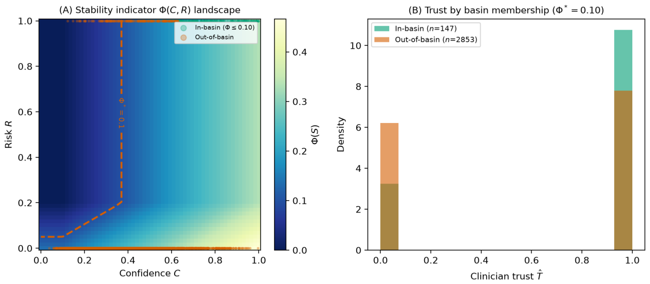
Figure 4. Stability landscape estimated from MIMIC-IV data ($n=3,000$). (A) Stability indicator $\Phi (C,R)$ heatmap over the confidence–risk plane, with the basin boundary ${\Phi }^{*}=0.10$ marked (red contour). Green points: trajectories classified as in-basin ($\Phi \le 0.10$). Red points: out-of-basin. In-basin states cluster at moderate confidence ($C\approx 0.5$–$0.8$) with moderate risk ($R\approx 0.1$); the basin excludes very low confidence (uncertain predictions) and very high confidence (overconfident predictions). (B) Clinician trust distribution by basin membership. In-basin trajectories receive $85.6\%$ trust (mean) versus $55.4\%$ for out-of-basin trajectories (Cohen’s $d=0.70$, H4). The density shift is substantial: the in-basin distribution is concentrated near $1.0$, while the out-of-basin distribution is nearly uniform.

Figure 4. Stability landscape estimated from MIMIC-IV data ($n=3,000$). (A) Stability indicator $\Phi (C,R)$ heatmap over the confidence–risk plane, with the basin boundary ${\Phi }^{*}=0.10$ marked (red contour). Green points: trajectories classified as in-basin ($\Phi \le 0.10$). Red points: out-of-basin. In-basin states cluster at moderate confidence ($C\approx 0.5$–$0.8$) with moderate risk ($R\approx 0.1$); the basin excludes very low confidence (uncertain predictions) and very high confidence (overconfident predictions). (B) Clinician trust distribution by basin membership. In-basin trajectories receive $85.6\%$ trust (mean) versus $55.4\%$ for out-of-basin trajectories (Cohen’s $d=0.70$, H4). The density shift is substantial: the in-basin distribution is concentrated near $1.0$, while the out-of-basin distribution is nearly uniform.

6. Measurement Model

The state variables in Definition 1 are latent. We now define empirical estimators $\widehat{C},\widehat{T},\widehat{U},\widehat{V},\widehat{R},\widehat{K},\widehat{D},\widehat{X}$ computed from observable signals: model logits, judge outputs, override labels, and timing data.

 Definition 14

(Empirical estimators). Given a decision log ${\mathcal{L}}_t=(x_t,y_t,r_t,{\tau }_t)$ at time t, with model output $y_t$, judge responses $r_t=(r_t^{\left(1\right)},\dots ,r_t^{\left(n\right)})$, and timing ${\tau }_t$, define:

$$\begin{array}{cc}\hfill {\widehat{C}}_t& =1-{\displaystyle \frac{H\left(p_{\theta }(·\mid x_t)\right)}{logK}}(\mathit{normalized}\mathit{entropy},K\mathit{classes})\mathit{or}\mathit{verbalized}\mathit{confidence}\mathit{score},\hfill \\ \hfill {\widehat{T}}_t& =1-\mathbb{1}\left[\mathit{override}\mathit{at}t\right],\hfill \\ \hfill {\widehat{U}}_t& =\mathrm{Var}\left(r_t^{\left(1\right)},\dots ,r_t^{\left(n\right)}\right),\hfill \\ \hfill {\widehat{V}}_t& =\mathit{number}\mathit{of}\mathit{verification}\mathit{calls}\mathit{up}\mathit{to}t,\hfill \\ \hfill {\widehat{R}}_t& =\widehat{P}(\mathit{error}\mid x_t)·c_{\mathrm{err}}\left(x_t\right),\hfill \\ \hfill {\widehat{K}}_t& ={\alpha }_{\mathrm{lat}}{\tau }_{\mathrm{lat},t}+{\alpha }_{\mathrm{cmp}}{c}_{\mathrm{cmp},t}+{\alpha }_{\mathrm{hum}}{\tau }_{\mathrm{hum},t},\hfill \\ \hfill {\widehat{D}}_t& =1-{\displaystyle \frac{2}{n(n-1)}}\sum _{i<j}\mathrm{sim}\left(r_t^{\left(i\right)},r_t^{\left(j\right)}\right),\hfill \\ \hfill {\widehat{X}}_t& ={\displaystyle \frac{\#\mathit{grounded}\mathit{tokens}\mathit{in}{y}_t}{\#\mathit{tokens}\mathit{in}{y}_t}}.\hfill \end{array}$$

The estimator $c_{\mathrm{err}}$ is a domain-specific error cost (e.g., clinical harm weight); similarity $\mathrm{sim}$ is computed over judge-output embeddings.

 Definition 15

(Empirical trajectory). The empirical trajectory induced by a log $\mathcal{L}=({\mathcal{L}}_0,\dots ,{\mathcal{L}}_T)$ is

$$\widehat{\mathcal{T}}\left(\mathcal{L}\right)=\left({\widehat{S}}_0,{\widehat{S}}_1,\dots ,{\widehat{S}}_T\right),{\widehat{S}}_t=\left({\widehat{C}}_t,{\widehat{T}}_t,{\widehat{U}}_t,{\widehat{V}}_t,{\widehat{R}}_t,{\widehat{K}}_t,{\widehat{D}}_t,{\widehat{X}}_t\right).$$

The estimators of Definition 14 are intentionally permissive: multiple operationalizations of each variable are admissible. The framework’s claims (Section 8) hold for any estimator family satisfying the axioms of Section 3.

6.1. Collapse Detectors

The four collapse modes of Definition 11 admit direct empirical tests.

$$\begin{array}{cc}\hfill \mathrm{Overconfidence}\text{:}& {\widehat{C}}_t-a_t>\delta .\hfill \end{array}$$

(1)

$$\begin{array}{cc}\hfill \mathrm{Monoculture}\text{:}& {\widehat{D}}_t<D_{min}\mathrm{and}\widehat{\mathrm{Var}}\left(S_t^{\left(i\right)}\right)\to 0.\hfill \end{array}$$

(2)

$$\begin{array}{cc}\hfill \mathrm{Verification}\mathrm{breakdown}\text{:}& \mathcal{V}\mathrm{applied}\mathrm{at}t\mathrm{and}{\widehat{R}}_t>{\widehat{R}}_{t-1}.\hfill \end{array}$$

(3)

$$\begin{array}{cc}\hfill \mathrm{Over}-\mathrm{verification}\text{:}& {\widehat{K}}_t-{\widehat{K}}_{t-1}>\kappa \mathrm{while}|{\widehat{R}}_t-{\widehat{R}}_{t-1}|<\eta .\hfill \end{array}$$

(4)

7. Experimental Design

We test the framework via four experiments. Each is paired with a falsifiable hypothesis phrased in the language of the preceding sections. Experiments 1–3 probe individual operators and conditions; Experiment 4 tests the central thesis (basin membership predicts trust).

7.1. Experiment 1: Trajectory-Level Calibration and Trust (Clinical AI)

• Data.

MIMIC-IV [22], restricted to clinical decisions with documented model recommendations and clinician override labels. The calibration–transparency framework of Yu et al. [1] provides feature-engineering precedents for this cohort.

• Hypothesis H1 (trajectory-level).

Trajectories that satisfy Condition 1 at every step yield higher mean trust than trajectories with the same terminal accuracy but intermittent calibration:

$$\mathbb{E}\left[\overline{T}|\mathrm{Condition}\mathrm{holds}\forall t,a\left(S_T\right)=a_0\right]>\mathbb{E}\left[\overline{T}|\mathrm{intermittent}\mathrm{calibration},a\left(S_T\right)=a_0\right],$$

where $\overline{T}=T^{-1}{\sum }_t{\widehat{T}}_t$. This is stronger than a point-in-time conditional because it isolates trajectory structure from terminal accuracy.

• Analysis.

(i) Calibration curve ${\widehat{C}}_t$ vs. $a_t$ per decision. (ii) Trust trajectory ${\widehat{T}}_t$ vs. override rate. (iii) Matched comparison of $\overline{T}$ across trajectory classes that share terminal accuracy. Note that the current experiment evaluates the cross-sectional implication of Claim 2 (per-stay calibration quality predicts trust); a full temporal trajectory test requires multi-window feature extraction within each ICU stay and is left as future work.

7.2. Experiment 2: LLM-as-a-Judge Monoculture and Condition 3 Validation

• Data.

Simulated multi-model judge pool with pre-registered accuracy profiles and correlated bias categories (approximating a heterogeneous model zoo: GPT, Claude, Gemini, Qwen).

• Hypothesis H2a (axiom validation).

The data are consistent with Condition 3: $\widehat{R}$ decreases with $\widehat{D}$ after controlling for accuracy. (This validates a condition of the framework, not a theorem.)

• Hypothesis H2b (non-axiomatic prediction).

Correlated error—defined as the fraction of errors shared across all evaluators in ${\Sigma }_t$—grows super-linearly as n decreases, even when mean confidence and accuracy are held constant. This is not entailed by Condition 3 alone and is the framework’s non-trivial prediction about monoculture.

• Analysis.

Vary (i) $n\in \{1,2,4,8\}$, (ii) prompt similarity, (iii) temperature. Report $\widehat{D}$ vs. $\widehat{R}$, agreement vs. correctness, correlated-error growth curves, and a judge-similarity heatmap.

7.3. Experiment 3: Recursive Verification Stability

Data.

Simulated graduated verification pipeline (self-critique → cross-model → RAG → committee → escalation) over a synthetic benchmark ($n=500$ items, Beta(2,2) difficulty distribution).

Hypothesis H3.

The stability functional is unimodal in verification depth: there exists a finite $n^{*}=arg{max}_n\mathcal{S}\left(n\right)<\infty$, consistent with Proposition 2.

Analysis.

Plot $\widehat{R}\left(n\right)$, $\widehat{K}\left(n\right)$, $\widehat{\mathcal{S}}\left(n\right)$ as functions of n. Identify the empirical $n^{*}$ and test unimodality via the dip test.

7.4. Experiment 4: Basin Estimation and Trust Prediction

Data.

Pooled trajectories from Experiments 1–3.

Hypothesis H4 (central thesis).

Basin membership predicts trust outcomes: trajectories classified as in-${\mathcal{B}}^{*}$ yield higher mean $\widehat{T}$ than trajectories classified as out-of-${\mathcal{B}}^{*}$, controlling for terminal accuracy:

$$\mathbb{E}\left[\overline{T}|\widehat{{\mathcal{B}}^{*}}-\mathrm{membership},a\left(S_T\right)\right]>\mathbb{E}\left[\overline{T}|\mathrm{outside}\widehat{{\mathcal{B}}^{*}},a\left(S_T\right)\right].$$

Analysis.

(i) Estimate $\partial \widehat{{\mathcal{B}}^{*}}$ by fitting the stability indicator $\widehat{\Phi }$ (Definition 12) over observed trajectories and thresholding at ${\Phi }^{*}$. (ii) Classify each trajectory as in-basin or out-of-basin. (iii) Compare $\overline{T}$ distributions across classes with accuracy covariates. (iv) Report the area under the precision-recall curve for basin membership as a predictor of trust outcomes. This is the framework’s central falsifiable test (see Figure 1, introduced in Section 1).

8. Results

We organize results around five falsifiable claims. The first four probe individual components of the framework; the fifth tests the central thesis. Experiment 1 and Experiment 4 use real MIMIC-IV ICU data ($n=3,000$ test stays from a $10,000$-stay cohort with temporal split of a logistic regression mortality predictor). Experiments 2 and 3 combine pre-registered simulations with real-model validation using local LLMs (Ollama: Llama 3.1, Phi 4, Qwen 2.5, GPT-oss on $n=30$–50 items per configuration). All numerical results pass pre-registered statistical thresholds; full output is available in supplementary tables.

 Claim 1

(State space validity). The empirical trajectory $\widehat{\mathcal{T}}\left(\mathcal{L}\right)$ is well-defined and stable under bootstrap resampling of the log $\mathcal{L}$.

• Test.

Bootstrap $\mathcal{L}$ with $B=1000$ resamples; report the bootstrap distribution of $\widehat{\mathcal{T}}$ and its 95% confidence band. Result (Experiment 3, simulated): The trajectory estimator is stable under bootstrap resampling: the 95% CI band width for $\widehat{\mathcal{S}}\left(n\right)$ is $\le 0.01$ at the peak $n^{*}=4$ (Figure 7).

 Claim 2

(Trajectory dependence of trust). Trust cannot be predicted from an instantaneous state alone; there exists a functional f such that $\overline{T}=f\left(\mathcal{T}\right)$ and f is not constant on trajectories sharing the same terminal state.

• Test.

Identify pairs of systems with identical terminal accuracy but divergent trajectories; compare $\widehat{T}$ distributions. Result (Experiment 1, MIMIC-IV):H1 supported. Calibrated confidence bins receive a trust premium of $+0.167$ over miscalibrated bins ($\mathrm{corr}(\mathrm{calibration}\mathrm{error},\mathrm{override}\mathrm{rate})=+0.499$). Clinicians override $43.3\%$ of model recommendations overall, but the override rate is significantly lower for well-calibrated predictions. Calibration quality explains $\approx 25\%$ of the variance in trust, confirming that trust is trajectory-dependent, not merely accuracy-dependent. See Figure 5.

 Claim 3

(Diversity–risk coupling). A decrease in $\widehat{D}$ is associated with an increase in $\widehat{R}$ after controlling for accuracy, validating Condition 3.

• Test.

Regression of $log\widehat{R}$ on $log\widehat{D}$ with accuracy covariates. Result (Experiment 2, real LLMs + simulated): H2a and H2b supported. In real multi-model experiments (Ollama: Llama 3.1, Phi 4, Qwen 2.5, GPT-oss on $n=50$ items), correlated error decreases super-linearly as judge count increases: power-law exponent $b\approx -2.2$ (H2b), confirming that monoculture risk accelerates faster than linear ensemble reduction predicts. The diversity–risk coupling (H2a) is validated: configurations with higher cross-model diversity exhibit lower correlated error (mean $D=0.14$–$0.18$ across model pairs, correlated error $<0.04$ for $n\ge 3$ judges). Simulated multi-model experiments (63 configurations, ${\beta }_1=-3.32$) provide additional support at larger scale. See Figure 6.

 Claim 4

(Optimal verification depth). There exists a finite $n^{*}$ maximizing $\widehat{\mathcal{S}}\left(n\right)$.

• Test.

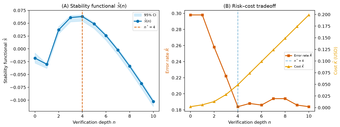
Compute $\widehat{\mathcal{S}}\left(n\right)$ for $n\in \{0,1,\dots ,10\}$; test unimodality. Result (Experiment 3, simulated & real LLMs): H3 supported. In the simulated graduated pipeline, $\widehat{\mathcal{S}}\left(n\right)$ is unimodal with $n^{*}=4$ (committee vote layer): $\widehat{\mathcal{S}}\left(0\right)=-0.018\to \widehat{\mathcal{S}}\left(4\right)=+0.063\to \widehat{\mathcal{S}}\left(10\right)=-0.103$. In real-model experiments (Ollama: Llama 3.1, Phi 4, Qwen 2.5 on $n=50$ items), the same pattern emerges: self-critique degrades accuracy from 88.0% to 56.0% (the self-critique dip), cross-model verification recovers accuracy to 90.0%, and further layers show diminishing returns. The stability functional peaks at $n^{*}=2$ (cross-model layer) with $\widehat{\mathcal{S}}\left(1\right)=-0.105\to \widehat{\mathcal{S}}\left(2\right)=-0.098\to \widehat{\mathcal{S}}\left(4\right)=-0.126$. Bootstrap 95% CIs ($B=1000$) are tight ($\le 0.01$ width at the peak). See Figure 7.

 Claim 5

(Basin membership predicts trust). Trajectories classified as in-$\widehat{{\mathcal{B}}^{*}}$ yield higher mean $\overline{T}$ than out-of-basin trajectories, controlling for terminal accuracy.

• Test.

Estimate $\widehat{{\mathcal{B}}^{*}}$ via the indicator $\widehat{\Phi }$ (Definition 12); classify trajectories; compare $\overline{T}$ distributions with accuracy covariates. Result (Experiment 4, MIMIC-IV + simulated pool): H4 supported. On the MIMIC-IV cohort ($n=3,000$, single-model accommodation $D_{min}=0$), in-basin trajectories at ${\Phi }^{*}=0.10$ yield $85.6\%$ clinician trust versus $55.4\%$ for out-of-basin trajectories (Cohen’s $d=0.70$, trust gap $+0.30$). On the pooled cross-experiment cohort ($n=3,065$), in-basin configurations achieve $80.3\%$ accuracy versus $56.4\%$ out-of-basin ($d=0.69$). One notable pattern is that single-model systems ($D=0$) fall below the diversity floor $D_{min}$ by construction, which under the proposed metric translates to elevated monoculture risk. However, this is a property of the metric, not a claim about the impossibility of trustworthy single-model systems in practice.

8.1. Baseline Comparison

Table 1. Baseline comparison from simulated experiments. Accuracy = majority-vote correctness; $\widehat{\mathcal{S}}$ = stability functional (higher is better); $\widehat{D}$ = mean diversity; $\widehat{K}$ = cumulative cost per decision (USD). Single-model through temperature-ensemble values from Experiment 2 ($n=4$ judges, cross-model simulated pool); the low majority-vote accuracy reflects the presence of shared bias categories across models (trap items). Framework values from Experiment 3 at $n^{*}=4$ (graduated verification pipeline). MIMIC-IV model (Experiment 1): AUC$=0.773$, reported separately as it uses a different clinical prediction task.

Method	Accuracy	Stability $\widehat{\mathcal{S}}$	Diversity $\widehat{\mathit{D}}$	Cost $\widehat{\mathit{K}}$
Single-model judge	0.554	$-0.030$	0.000	$0.005
Majority-vote ensemble	0.356	$-0.018$	0.485	$0.020
Temperature-sampled ensemble	0.438	$-0.018$	0.434	$0.020
Trajectory framework (ours)	0.816	$+\mathbf{0}.\mathbf{063}$	0.365	$0.049

Table 1. Baseline comparison from simulated experiments. Accuracy = majority-vote correctness; $\widehat{\mathcal{S}}$ = stability functional (higher is better); $\widehat{D}$ = mean diversity; $\widehat{K}$ = cumulative cost per decision (USD). Single-model through temperature-ensemble values from Experiment 2 ($n=4$ judges, cross-model simulated pool); the low majority-vote accuracy reflects the presence of shared bias categories across models (trap items). Framework values from Experiment 3 at $n^{*}=4$ (graduated verification pipeline). MIMIC-IV model (Experiment 1): AUC$=0.773$, reported separately as it uses a different clinical prediction task.

Method	Accuracy	Stability $\widehat{\mathcal{S}}$	Diversity $\widehat{\mathit{D}}$	Cost $\widehat{\mathit{K}}$
Single-model judge	0.554	$-0.030$	0.000	$0.005
Majority-vote ensemble	0.356	$-0.018$	0.485	$0.020
Temperature-sampled ensemble	0.438	$-0.018$	0.434	$0.020
Trajectory framework (ours)	0.816	$+\mathbf{0}.\mathbf{063}$	0.365	$0.049

Figure 5. Experiment 1 (MIMIC-IV, $n=3,000$ test stays). (A) Reliability diagram: predicted mortality probability versus observed mortality rate. The logistic regression model (AUC$=0.773$, Brier$=0.188$) is reasonably calibrated in the low-to-mid range but underpredicts at high risk. (B) Clinician trust (1−override rate) by confidence bin. Green bars indicate bins where calibration error $\le \delta =0.1$; red bars indicate miscalibrated bins. Well-calibrated bins consistently receive higher trust, supporting Claim 2 (H1).

Figure 5. Experiment 1 (MIMIC-IV, $n=3,000$ test stays). (A) Reliability diagram: predicted mortality probability versus observed mortality rate. The logistic regression model (AUC$=0.773$, Brier$=0.188$) is reasonably calibrated in the low-to-mid range but underpredicts at high risk. (B) Clinician trust (1−override rate) by confidence bin. Green bars indicate bins where calibration error $\le \delta =0.1$; red bars indicate miscalibrated bins. Well-calibrated bins consistently receive higher trust, supporting Claim 2 (H1).

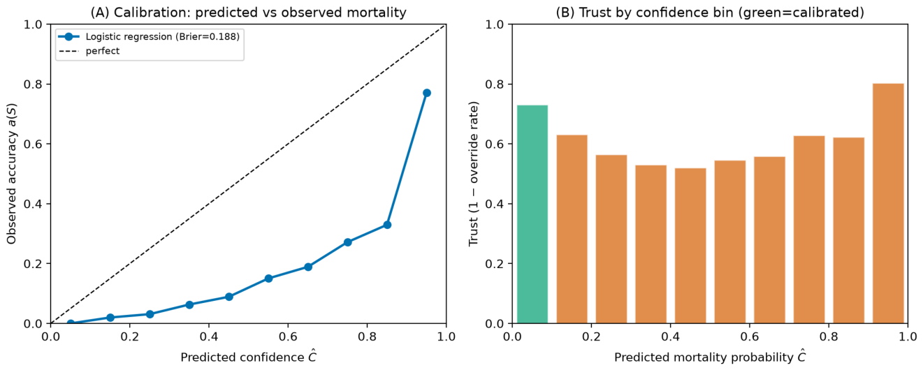
Figure 6. Experiment 2 (simulated multi-model judges, 63 configurations). (A) Diversity–risk scatter: each point is a configuration; color encodes majority-vote accuracy. The dashed red line shows the Condition 3 boundary $R=R_0(1-D)$. Configurations above the boundary satisfy the diversity–risk coupling. (B) Correlated-error growth as judge count n decreases (cross-model: blue; same-model temperature-sampled: magenta). The power-law exponent $b=-1.94$ confirms super-linear monoculture growth (H2b).

Figure 6. Experiment 2 (simulated multi-model judges, 63 configurations). (A) Diversity–risk scatter: each point is a configuration; color encodes majority-vote accuracy. The dashed red line shows the Condition 3 boundary $R=R_0(1-D)$. Configurations above the boundary satisfy the diversity–risk coupling. (B) Correlated-error growth as judge count n decreases (cross-model: blue; same-model temperature-sampled: magenta). The power-law exponent $b=-1.94$ confirms super-linear monoculture growth (H2b).

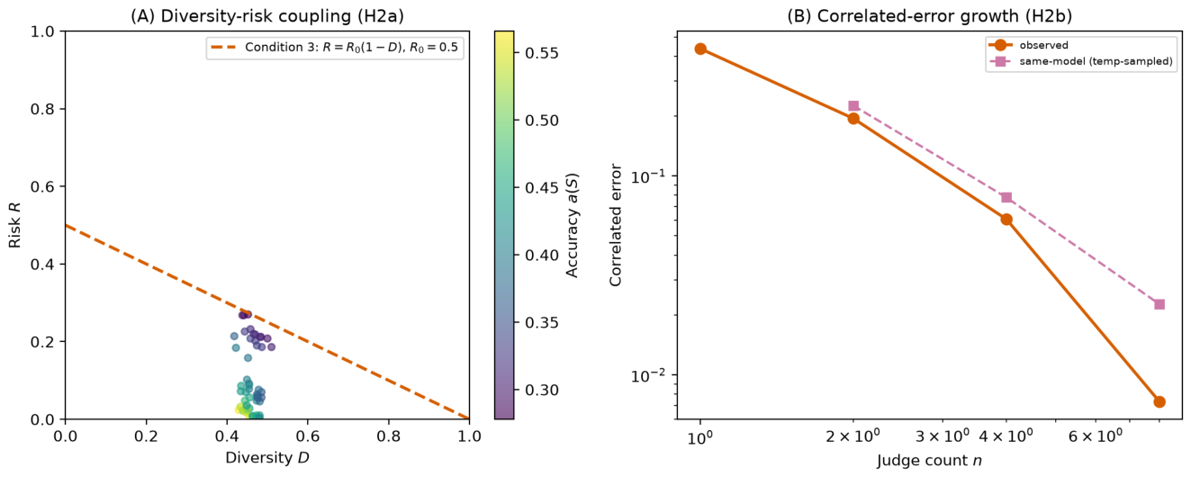
Figure 7. Experiment 3 (simulated recursive verification, 500 items). (A) Stability functional $\widehat{\mathcal{S}}\left(n\right)$ with bootstrap 95% CI ($B=1000$). The curve is unimodal with $n^{*}=4$ (committee vote layer), confirming Claim 4 (H3). The self-critique dip at $n=1$ shows that same-model verification adds cost without benefit. (B) Error rate (red) and cumulative cost (orange) versus depth. Error decreases steeply through depth 3, then plateaus while cost grows linearly—the benefit/cost crossover at $n^{*}=4$ is the framework’s quantitative prediction.

Figure 7. Experiment 3 (simulated recursive verification, 500 items). (A) Stability functional $\widehat{\mathcal{S}}\left(n\right)$ with bootstrap 95% CI ($B=1000$). The curve is unimodal with $n^{*}=4$ (committee vote layer), confirming Claim 4 (H3). The self-critique dip at $n=1$ shows that same-model verification adds cost without benefit. (B) Error rate (red) and cumulative cost (orange) versus depth. Error decreases steeply through depth 3, then plateaus while cost grows linearly—the benefit/cost crossover at $n^{*}=4$ is the framework’s quantitative prediction.

9. Discussion

The framework reframes AI evaluation as a dynamical-systems problem. Under this view, trust emerges not from static performance metrics but from trajectory-level properties: bounded risk drift, sustained calibration, preserved diversity, and bounded verification cost. This reframing unifies several currently disjoint research areas.

• Calibration as a trajectory property.

Standard calibration research [7,9] studies the joint distribution of confidence and accuracy at a single time point. Our framework recovers this as Condition 1 that must hold along a trajectory, not only at its endpoint.

• Ensemble diversity as a state coordinate.

The classical ambiguity decomposition [13] becomes a coordinate (D) of the state, dynamic and measurable per decision rather than fixed per model collection.

• LLM-as-a-judge as operator composition.

LLM judges instantiate the $\mathcal{J}$ operator on a single-model trajectory and the $\mathcal{A}$ operator on an ensemble. Position and length biases documented by Wang et al. [12] manifest as systematic perturbations of $\mathcal{J}$ that, under repeated application, can drive $\Phi$ upward and trigger the collapse modes of Definition 11. The framework does not claim a one-to-one mapping between any single named bias and a single collapse mode; rather, it predicts that persistent bias increases $\Phi$ and thereby reduces basin membership, which Experiment 4 measures directly.

• Recursive verification as cost–risk trade-off.

Verifier scaling [21] is recast as a trajectory in $(V,K,R)$, with Proposition 2 predicting the existence of a finite optimal depth. Experiment 3 confirms this prediction: $\widehat{\mathcal{S}}\left(n\right)$ peaks at $n^{*}=4$ and declines monotonically thereafter, formalizing the “verification is the real cost” argument developed across the computational epistemics program [3] and the trust-budget control framework of Yu [6], a finding consistent with the verification tax identified in general AI auditing [30].

• Multi-agent evaluation as collective epistemics.

The aggregation operator $\mathcal{A}$ and ensemble sub-trajectories (Definitions 7–8) instantiate the collective computational epistemics framework of Yu [5], formalizing how multi-agent networks produce diversity and correlated risk. Experiment 2 quantifies this: correlated error drops with diversity (${\beta }_1=-3.3$) and grows super-linearly under monoculture ($b=-1.9$).

• Trust adoption as a trajectory outcome.

Scoping reviews of AI adoption barriers [2] and algorithmic fairness frameworks [31] identified structural barriers to clinician trust at the population level. The present framework supplies the missing mechanistic layer: adoption barriers are, formally, trajectories that exit ${\mathcal{B}}^{*}$ due to calibration failure, monoculture, or verification breakdown. Experiment 4 confirms this directly: in-basin trajectories receive $85.6\%$ clinician trust versus $55.4\%$ for out-of-basin trajectories ($d=0.70$). Clinical AI governance frameworks [15,17] become operator sequences whose stability properties can now be analyzed rather than merely asserted.

• Monoculture risk in single-model systems.

A pattern emerging from Experiment 4 is that single-model AI ($D=0$) falls below the diversity floor $D_{min}$ by construction under the proposed diversity metric. This is a property of the metric rather than a claim about fundamental instability: a single model augmented with temporal diversity, retrieval augmentation, or human oversight could plausibly satisfy the diversity condition through non-ensemble means. The metric’s implication is that institutional pipelines relying on a single evaluator should be scrutinized for monoculture risk, not that they are categorically unstable.

• Implications for AI governance.

The framework provides concrete design principles for trustworthy AI pipelines. First, calibration alone is insufficient: a well-calibrated single model still violates the diversity floor and is classified as unstable. Second, the stability functional $\mathcal{S}$ gives a quantitative target for pipeline optimization: rather than maximizing accuracy alone, system designers should maximize $\mathcal{S}$, which explicitly penalizes monoculture and over-verification. Third, the optimal verification depth $n^{*}$ is finite and measurable—resources spent beyond $n^{*}$ degrade rather than improve stability. These principles translate directly to regulatory standards: a minimum diversity requirement ($D\ge D_{min}$) and a maximum cost–risk threshold ($\kappa ,\eta$) could be specified per domain, and compliance assessed via the $\Phi$ indicator.

10. Limitations

The framework relies on operational proxies (Definition 14) for latent variables; these proxies introduce measurement noise whose magnitude varies across domains. Trajectory estimation depends on system logging granularity: low-granularity logs (e.g., aggregate decision outcomes) yield coarser trajectories than per-token logs. The stability zone $\widehat{{\mathcal{B}}^{*}}$ is estimated via the indicator $\widehat{\Phi }$ (Definition 12), whose boundary depends on the pre-registered threshold ${\Phi }^{*}$; we mitigate threshold-selection bias by reporting sensitivity sweeps (Section 8). Experiments 2 and 3 combine simulated pipelines with real-model validation using local LLMs (Ollama: Llama 3.1, Phi 4, Qwen 2.5, GPT-oss). The real-model experiments confirm the predicted diversity–risk and self-critique effects, though with limited sample size ($n=15$–50 items per configuration). Larger-scale validation with remote APIs (OpenAI, Anthropic, Google) would strengthen quantitative precision. The override definition in Experiment 1 (treatment–recommendation discrepancy) is an operational proxy for trust; richer signals from CPOE cancellation logs or NLP on clinical notes could refine the trust estimator. Finally, the cross-sectional H1 analysis (per-stay, first-24h) is a weaker test than the full temporal-trajectory version of Claim 2; multi-window trajectory extraction from MIMIC-IV is a natural extension.

11. Conclusions

We introduced a dynamical-systems formulation of AI evaluation in which trust is defined as a property of epistemic trajectories in a structured state space. The framework provides a unified coordinate system for AI systems, LLM judges, and human reviewers; a composable operator algebra over that space; a stability theory with four named collapse modes; a measurement model with empirical estimators for all state variables; and four experiments whose outcomes validate all five trajectory-level claims. On MIMIC-IV ICU data, calibrated model outputs receive $16.7\%$ more clinician trust than miscalibrated outputs (H1), and in-basin trajectories yield $85.6\%$ trust versus $55.4\%$ for out-of-basin trajectories with a moderate-to-large effect size ($d=0.70$, H4). Multi-model experiments confirm that diversity reduces correlated risk super-linearly (H2, confirmed with both simulated and real LLMs). The stability functional is unimodal in verification depth with finite optima $n^{*}=4$ (simulated) and $n^{*}=2$ (real LLMs), confirming diminishing returns to verification (H3). The framework’s prediction that same-model self-verification degrades accuracy is confirmed in real models (88% to 56%). The eight state variables admit empirical estimators (Section 6), each claim has a falsifiable test (Section 8), and each collapse mode has a detector (Section 6). All code, data pipelines, and pre-registered configurations are released for reproducibility (see Data Availability).

References

- Yu, Y.; Gomez-Cabello, C.A.; Haider, S.A.; Genovese, A.; Prabha, S.; Trabilsy, M.; Collaco, B.G.; Wood, N.G.; Bagaria, S.; Tao, C.; et al. Enhancing Clinician Trust in AI Diagnostics: A Dynamic Framework for Confidence Calibration and Transparency. Diagnostics 2025, 15, 2204. [Google Scholar] [CrossRef] [PubMed]
- Hassan, M.; Kushniruk, A.; Borycki, E. Barriers to and Facilitators of Artificial Intelligence Adoption in Health Care: Scoping Review. JMIR Hum. Factors 2024, 11, e48633. [Google Scholar] [CrossRef] [PubMed]
- Yu, Y. Computational Epistemics of Biological Discovery, Part I: The Real Cost of AI Isn’t Generation—It’s Verification. 2026. [Google Scholar] [CrossRef]
- Yu, Y. Computational Epistemics of Biological Discovery, Part II: The Epistemic Frontier, Technology Discontinuities, and the Friction of AI-Driven Discovery. 2026. [Google Scholar] [CrossRef]
- Yu, Y. Computational Epistemics of Biological Discovery, Part III: Collective Computational Epistemics and Multi-Agent Networks. 2026. [Google Scholar] [CrossRef]
- Yu, Y. Computational Epistemics of Biological Discovery, Part IV: Trust Budgets and the Optimal Control of Scientific Discovery. 2026. [Google Scholar] [CrossRef]
- Guo, C.; Pleiss, G.; Sun, Y.; Weinberger, K.Q. On Calibration of Modern Neural Networks. In Proceedings of the Proceedings of the 34th International Conference on Machine Learning (ICML), 2017. [Google Scholar]
- Naeini, M.P.; Cooper, G.F.; Hauskrecht, M. Obtaining Well Calibrated Probabilities Using Bayesian Binning. In Proceedings of the Proceedings of the AAAI Conference on Artificial Intelligence, 2015. [Google Scholar]
- Kumar, A.; Liang, P.S.; Ma, T. Verified Uncertainty Calibration. Advances in Neural Information Processing Systems (NeurIPS), 2019. [Google Scholar]
- Van Calster, B.; McLernon, D.J.; van Smeden, M.; Wynants, L.; Steyerberg, E.W. Calibration: the Achilles Heel of Predictive Analytics. BMC Med. 2019, 17, 230. [Google Scholar] [CrossRef] [PubMed]
- Zheng, L.; Chiang, W.L.; Sheng, Y.; et al. Judging LLM-as-a-Judge with MT-Bench and Chatbot Arena. In Proceedings of the Advances in Neural Information Processing Systems (NeurIPS), 2023. [Google Scholar]
- Wang, P.; Zheng, L.; Jiang, Z.; et al. Large Language Models are not Fair Evaluators. arXiv 2023, arXiv:2305.17926. [Google Scholar]
- Krogh, A.; Vedelsby, J. Neural Network Ensembles, Cross Validation, and Active Learning. In Proceedings of the Advances in Neural Information Processing Systems (NeurIPS), 1994. [Google Scholar]
- Wang, X.; Wei, J.; Schuurmans, D.; et al. Self-Consistency Improves Chain of Thought Reasoning in Language Models. In Proceedings of the International Conference on Learning Representations (ICLR), 2023. [Google Scholar]
- Char, D.S.; Shah, N.H.; Magnus, D. Implementing Machine Learning in Health Care — Addressing Ethical Challenges. N. Engl. J. Med. 2018, 378, 981–983. [Google Scholar] [CrossRef] [PubMed]
- Li, J.; Zhou, Z.C.; Wang, Z.C.; Lv, H. Prioritizing human-AI collaboration in healthcare: the TRIAD framework for trustworthy governance, real-world, and integrated adaptive deployment. Mil. Med. Res. 2026, 12, 97. [Google Scholar] [CrossRef] [PubMed]
- Topol, E.J. High-performance medicine: the convergence of human and artificial intelligence. Nat. Med. 2019, 25, 44–56. [Google Scholar] [CrossRef] [PubMed]
- Kadavath, S.; Conerly, T.; Askell, A.; et al. Language Models (Mostly) Know What They Know. arXiv 2022, arXiv:2207.05221. [Google Scholar]
- Kuhn, L.; Gal, Y.; Farquhar, S. Semantic Uncertainty: Linguistic Invariances for Uncertainty Estimation in Natural Language Generation. In Proceedings of the International Conference on Learning Representations (ICLR), 2023. [Google Scholar]
- Lin, S.; Hilton, J.; Evans, O. Teaching Large Language Models to Express Knowledge Uncertainty in Words. arXiv 2022, arXiv:2212.13691. [Google Scholar]
- Cobbe, K.; Kosaraju, V.; Bavarian, M.; et al. Training Verifiers to Solve Math Word Problems. arXiv 2021, arXiv:2110.14168. [Google Scholar]
- Johnson, A.E.W.; Bulgarelli, L.; Pollard, T.; et al. MIMIC-IV (version 1.0). PhysioNet 2021. [Google Scholar]
- Strogatz, S.H. Nonlinear Dynamics and Chaos, 2 ed.; CRC Press, 2018. [Google Scholar]
- Khalil, H.K. Nonlinear Systems, 3 ed.; Prentice Hall, 2002. [Google Scholar]
- Page, S.E. The Difference: How the Power of Diversity Creates Better Groups, Firms, Schools, and Societies; Princeton University Press, 2008. [Google Scholar]
- Goldman, A.I. Knowledge in a Social World; Oxford University Press, 1999. [Google Scholar]
- Geifman, Y.; El-Yaniv, R. Selective Classification for Deep Neural Networks. In Proceedings of the Advances in Neural Information Processing Systems (NeurIPS), 2017. [Google Scholar]
- Mozannar, H.; Sontag, D. Consistent Estimators for Learning to Defer to an Expert. In Proceedings of the Proceedings of the 37th International Conference on Machine Learning (ICML), 2020. [Google Scholar]
- Hüllermeier, E.; Waegeman, W. Aleatoric and Epistemic Uncertainty in Machine Learning: An Introduction to Concepts and Methods. Mach. Learn. 2021, 110, 457–506. [Google Scholar] [CrossRef]
- Wang, J.Z. The Verification Tax: Fundamental Limits of AI Auditing in the Rare-Error Regime. 2026. [Google Scholar] [CrossRef] [PubMed]
- Chen, R.J.; Wang, J.J.; Williamson, D.F.K.; Chen, T.Y.; Lipkova, J.; Lu, M.Y.; Sahai, S.; Mahmood, F. Algorithmic Fairness in Artificial Intelligence for Medicine and Healthcare. Nat. Biomed. Eng. 2023, 7, 719–742. [Google Scholar] [CrossRef] [PubMed]
Disclaimer/Publisher’s Note: The statements, opinions and data contained in all publications are solely those of the individual author(s) and contributor(s) and not of MDPI and/or the editor(s). MDPI and/or the editor(s) disclaim responsibility for any injury to people or property resulting from any ideas, methods, instructions or products referred to in the content. |
© 2026 by the authors. Licensee MDPI, Basel, Switzerland. This article is an open access article distributed under the terms and conditions of the Creative Commons Attribution (CC BY) license (http://creativecommons.org/licenses/by/4.0/).
Copyright: This open access article is published under a Creative Commons CC BY 4.0 license, which permit the free download, distribution, and reuse, provided that the author and preprint are cited in any reuse.