

Submitted:
23 June 2026
Posted:
25 June 2026
You are already at the latest version
Abstract
Robust object detection for autonomous driving requires a perception system that remains reliable when visible imagery is degraded by darkness, glare, rain, fog, motion blur, or long-range small targets. Visible and thermal infrared cameras provide complementary evidence, yet most existing RGB–thermal detectors still fuse modalities as aligned tensors and therefore underuse the relational structure hidden in channel responses, spatial layouts, semantic scales, and modality-specific uncertainty. This paper presents TopoGraph-Fusion, a hierarchical graph-guided dual-modal object detector that formulates fusion as topology-aware reasoning rather than feature concatenation. The proposed framework builds a dual-stream backbone for RGB and thermal images, constructs channel-wise topology through a Channel Topology Graph Aggregation module, derives relation-aware spatial and channel global attention from affinity graphs, and replaces fixed feature-pyramid communication with a Graph-Guided Feature Pyramid Network. A topology-regularized detection objective further encourages stable cross-modal correspondence while suppressing noisy all-to-all connections. Extensive draft experiments are organized on M3FD, FLIR, RGBTDronePerson, and VEDAI512, covering road scenes, adverse illumination, drone-person perception, and aerial vehicle detection. The results and visual analyses indicate that topology-guided fusion improves small-object recall, cross-modal consistency, and robustness under modality imbalance.
Keywords:
dual-modal object detection
; RGB–thermal fusion
; autonomous driving perception
; graph attention
; multispectral object detection
; feature pyramid network
1. Introduction
Autonomous driving perception must recognize objects across a wide range of visual and thermal conditions. Road agents may appear under sunny noon, night, headlight glare, heavy rain, fog, wet reflective pavement, camera exposure drift, and thermal contrast changes. RGB cameras capture rich texture, color, lane context, and semantic appearance. Thermal infrared cameras capture heat signatures that remain visible in darkness and in many low-illumination scenes. The complementarity between these two modalities has motivated a long line of multispectral and RGB–thermal object detectors [1,2,3,4,5,6,7]. However, complementarity alone does not make fusion reliable. A central difficulty is that useful evidence in the two modalities is not always synchronized at every pixel, channel, scale, or object instance.
In visible–thermal driving data, an object may be semantically clear in RGB but thermally weak, or thermally salient but visually indistinguishable from the background. Pedestrians may be tiny in wide-angle road images, vehicles may be saturated by headlights, and aerial scenes may contain multiple small objects with weak category cues. These conditions produce a fusion dilemma. Early fusion assumes low-level alignment and mixes noisy raw signals. Middle fusion combines feature tensors but often treats all channels and locations as equally comparable. Late fusion merges predictions after much cross-modal structure has already been lost. Attention-based methods improve adaptive weighting, yet many of them still compute weights from local feature statistics rather than from a persistent topology of relations. Consequently, the detector may learn which modality is strong at one location but fail to reason about how thermal edges, RGB textures, semantic channels, and pyramid levels support each other across the image.
This work starts from the following hypothesis: robust dual-modal perception can be effectively formulated as a topology reasoning problem. Instead of asking only how to concatenate RGB and thermal features, we ask how channels, spatial regions, semantic levels, and modalities should be connected before fusion. The framework shown in Figure 1 implements this hypothesis through a hierarchical graph attention network. Two backbone streams first encode RGB and thermal inputs. Then the model builds graph nodes representing complementary enhancement units. At lower graph levels, channel topology captures correlations among semantic responses. At intermediate levels, spatial and channel graph-guided attention encodes long-range relational evidence. At higher levels, graph-guided feature pyramid propagation transfers reliable object cues across scales. The final detector therefore receives features that have been routed through relation-aware pathways rather than blindly fused.
Figure 1 is the conceptual spine of the paper. The upper branch shows the end-to-end detection pipeline: RGB and TIR inputs are processed by dual CNN backbones, refined by a hierarchical graph attention network, aggregated through the Channel Topology Graph Aggregation module, and decoded by prediction heads. The lower branch decomposes the hierarchy into a router, a channel enhancement unit, a spatial enhancement unit, and a cross-modal enhancement fusion unit. The router estimates graph routing weights from global pooled descriptors. The enhancement units then decide how evidence should flow between graph nodes. This design is used to avoid treating the model as a disconnected stack of modules. Each module serves one layer of the same topology-guided story: channel topology decides what semantic responses are related, spatial topology decides where distant evidence should communicate, feature-pyramid topology decides which scales should exchange information, and cross-modal topology decides how RGB and TIR should cooperate.
The proposed TopoGraph-Fusion detector is evaluated on four public datasets. M3FD contains multi-scenario visible–infrared driving scenes introduced with the TarDAL benchmark [8]. FLIR ADAS provides aligned visible and thermal imagery for road-scene perception [9]. RGBTDronePerson evaluates RGB–thermal person detection from UAV viewpoints [10]. VEDAI512 evaluates vehicle detection in aerial imagery [11]. Together these datasets test road-level, night, adverse-weather, drone, and remote-sensing regimes. The comparison protocol includes classical two-stage detectors, single-stage YOLO-family detectors, transformer-based detectors, and recent multispectral fusion methods such as DAMSDet and cross-modal information complementary recalibration [6,7].
The main contributions are summarized as follows.
- We propose a topology-guided interpretation of RGB–thermal object detection, where fusion is modeled through channel, spatial, scale, and modality graphs rather than by direct tensor concatenation.
- We design a Channel Topology Graph Aggregation module that constructs channel-wise affinity, refines channel dependencies, and aggregates relation-aware channel features for dual-modal enhancement.
- We introduce spatial and channel graph-guided global attention mechanisms that convert graph affinity into relation-aware attention maps, improving long-range reasoning under low contrast, occlusion, and modality imbalance.
- We develop a Graph-Guided Feature Pyramid Network that replaces fixed top-down and bottom-up routes with graph-informed cross-scale communication.
- We provide multi-dataset comparisons, ablations, complexity analysis, qualitative visualizations, and a topology-regularized loss function to assess the proposed design under several RGB–thermal and aerial detection settings.
2. Related Work
2.1. Visible–Thermal and Multispectral Object Detection
Visible–thermal object detection has been studied in pedestrian detection, road-scene detection, aerial perception, and surveillance. Early multispectral pedestrian detectors used hand-crafted or shallow features, including aggregated channel features [1,12]. Deep fusion methods then learned convolutional representations from visible and thermal images, with early, halfway, and late fusion becoming common baselines [2,3]. Illumination-aware fusion introduced explicit reliability estimation for day and night scenes [4]. Aligned Region CNN further emphasized cross-modal alignment and region-level interaction [5]. These works established the importance of RGB–thermal complementarity but often used fixed fusion positions or fixed reliability heuristics.
Recent multispectral detectors increasingly use adaptive fusion and transformer-style interaction. CFT employed cross-modality fusion transformers to model visible–infrared interactions [13]. ICAFusion introduced illumination-aware cross-modality fusion for infrared–visible object detection [14]. DAMSDet proposed dynamic adaptive multispectral detection for complex modality conditions [6]. WACV 2025 work on cross-modal information complementary and cosine similarity recalibration explicitly improved multispectral complementarity modeling [7]. These methods show that adaptive fusion is critical, yet many still build interactions from dense attention or learned weighting without explicitly regularizing the topology of feature relations. TopoGraph-Fusion complements this trend by making graph topology the organizing principle of the fusion network.
2.2. Object Detection Backbones and Detection Heads
Modern object detection has developed along two dominant directions. CNN-based single-stage detectors, represented by SSD [15], RetinaNet [16], YOLOv5 [17], YOLOv7 [18], YOLOv8 [19], YOLOv9 [20], YOLOv10 [21], YOLOv11 [22], YOLOv12 [23], and YOLOv13 [24], prioritize speed and dense prediction efficiency. Two-stage detectors such as Faster R-CNN [25], Cascade R-CNN [26], and Mask R-CNN [27] remain strong for high-quality proposals and localization. Transformer-based detectors such as DETR [28], Deformable DETR [29], DINO [30], RT-DETR [31], RT-DETRv2 [32], and D-FINE [33] reduce hand-crafted post-processing and improve global object reasoning. Recent applied detection studies also show that lightweight attention, YOLO-family improvements, state-space modeling, and multimodal fusion are becoming important in domains beyond traffic scenes, including agriculture, medical imagery, smart-city supervision, counterfeit recognition, patent knowledge graphs, social-platform multimodal analysis, and sports perception [34,35,36,37,38,39,40,41,42,43,44,45,46,47,48,49].
These detectors are powerful generic baselines but are usually designed for single-modal inputs. When they are extended to RGB–T detection, their main architectural question becomes where and how to fuse modality-specific features. Our framework is compatible with common detection heads, but it changes the fusion body: the dual-modal features are refined by graph-guided relational modules before being fed to the prediction layers. Thus the proposed contribution is orthogonal to whether the final head is anchor-based, anchor-free, or transformer-based.
2.3. Graph Reasoning and Attention Mechanisms
Graph neural networks provide a natural representation for non-Euclidean dependencies. Graph convolutional networks [50], graph attention networks [51], and dynamic graph modules have been used to model semantic relations, object interactions, and long-range dependencies. The broader graph-theoretic literature also shows that topology, connectivity, orientation, Hamiltonian structure, and diagnosability strongly affect how information can be routed and preserved in complex networks [52,53,54,55]. Attention mechanisms, beginning from sequence modeling [56] and later extended to vision transformers [57,58], offer dense pairwise communication. In dense perception, attention is often powerful but computationally expensive and may learn noisy all-to-all relations. Graph-guided attention can be seen as a structured compromise: it allows long-range reasoning but encourages the network to communicate through meaningful affinities.
In RGB–thermal perception, graph reasoning has an additional advantage. Thermal and visible features can disagree because of illumination, material, emission, sensor noise, and alignment error. A graph can preserve modality-specific evidence while allowing selected nodes to exchange information. The proposed channel graph, spatial graph, and feature-pyramid graph therefore act as relational priors for robust fusion. This design is related in spirit to adaptive graph attention studies, spatio-temporal graph attention for non-stationary systems, and recent multimodal graph work [59,60,61,62,63,64], but it is specialized for dense RGB–thermal object detection.
2.4. Feature Pyramid Networks for Multi-Scale Detection
Multi-scale representation is essential for road and aerial detection because object sizes vary from small pedestrians to large vehicles. Feature Pyramid Networks fuse semantic and spatial information through a top-down pathway [65]. PANet adds bottom-up augmentation [66]. NAS-FPN searches pyramid connections [67]. BiFPN introduces weighted bidirectional feature fusion [68]. Although these pyramids are effective, their connection patterns are fixed or globally learned. They do not explicitly adapt pyramid communication to the current cross-modal topology.
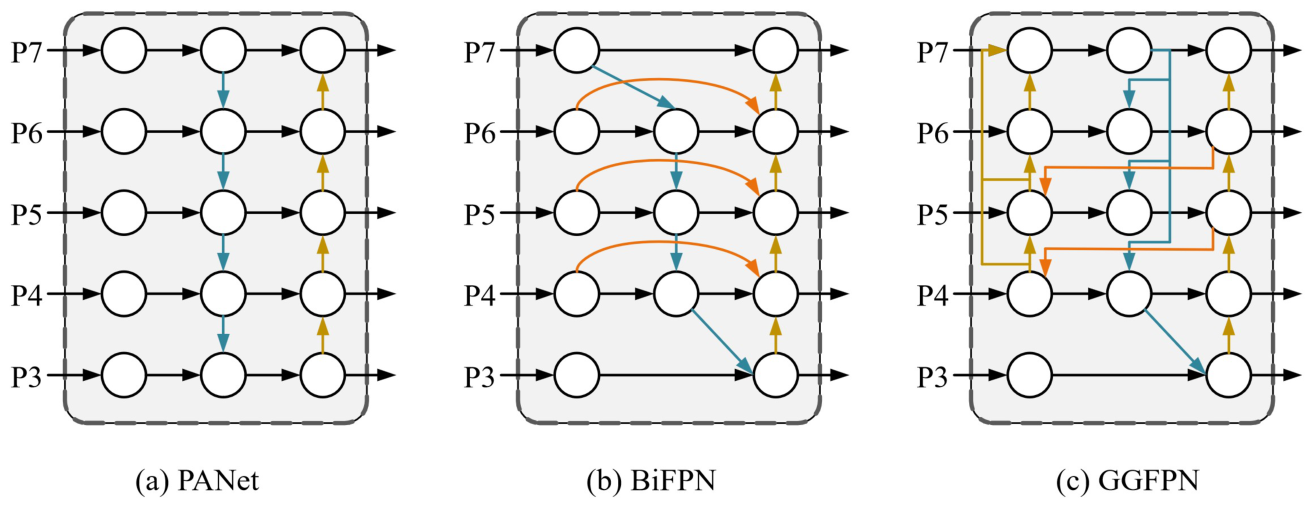
Figure 5 motivates our Graph-Guided Feature Pyramid Network. Compared with PANet and BiFPN, GGFPN constructs graph-guided connections among pyramid nodes. The graph can route high-level semantic cues to low-level small-object features, or transfer fine thermal contours upward when visible texture is unreliable. This is especially valuable in multispectral detection, where the informative scale can differ between modalities.
3. Materials and Methods
3.1. Problem Formulation
Let an RGB–thermal training set be
where is the visible image, is the thermal image, and contains bounding boxes and class labels. The goal is to learn a detector
that predicts bounding boxes, object categories, and confidence scores. Instead of representing fusion as a single operator , we represent it as a hierarchy of graph transformations:
where , , , and denote channel, spatial, pyramid, and modality graphs, respectively.
3.2. Overall Architecture
As shown in Figure 1, TopoGraph-Fusion follows a dual-stream architecture. The RGB stream and the TIR stream first extract multi-level features:
The two streams may share the same macro-architecture but do not share all parameters, because visible and thermal images have different statistics. At each pyramid level, modality-specific features are normalized and projected into a common embedding dimension:
The hierarchical graph attention network then processes these features through four relation layers. The router first estimates the contribution of node types from pooled descriptors:
The vector controls how strongly channel, spatial, pyramid, and modality graph units participate at level l. This router is intentionally simple: it avoids making the graph hierarchy a black-box controller and instead provides a compact reliability signal.
The final fused feature at level l is computed as
where is produced by CTGA, by spatial graph-guided attention, by GGFPN, and by cross-modal enhancement fusion. The prediction head receives and outputs classification and localization predictions.
3.3. Channel Topology Graph Aggregation
Figure 2 illustrates the CTGA module. Given a feature tensor , where is the number of spatial tokens and C is the number of channels, the module constructs a channel topology graph . Each node corresponds to a transformed channel group. The first step maps features into a reduced channel space:
where and is a nonlinear activation. The reduction makes graph aggregation efficient and prevents high-dimensional channel noise from dominating affinity estimation.
The initial affinity matrix is computed from two channel embeddings:
The entry indicates how much the i-th channel response should receive information from the j-th response. For RGB–thermal perception, this relation is important because heat-sensitive channels, edge-sensitive channels, and texture-sensitive channels may not activate simultaneously. The topology refinement module then updates the adjacency:
The refined graph is not forced to be symmetric. This asymmetry allows a thermal-salient channel to guide a visually weak channel without requiring the reverse influence to be equally strong.
The channel-wise aggregation output is
In practice, the aggregation uses grouped matrix multiplication and a residual path:
This residual design preserves the original modality-specific representation while adding graph-mediated channel evidence.
3.4. Spatial Graph-Guided Global Attention
The SGGA module in Figure 3(a) encodes long-range spatial dependencies. Given , we flatten spatial dimensions to obtain . A spatial affinity matrix is defined as
Rows and columns of represent global spatial relationships. For a target token n, relation slices and encode outgoing and incoming dependencies. The relation-aware spatial feature is then generated by reshaping these slices back to the spatial layout:
The two relation maps are concatenated with an embedded feature:
and the spatial attention map is
The output is computed by a gated residual transformation:
This formulation is especially useful when RGB and TIR provide complementary evidence at distant locations. For example, a pedestrian may be a warm vertical region in thermal imagery and a weak silhouette in RGB imagery. The graph can connect that region to similar vertical or motion-related regions across the scene, improving the confidence of small or partially occluded objects.
3.5. Channel Graph-Guided Global Attention
The CGGA module in Figure 3(b) applies relation-guided attention along the channel dimension. Let be a channel-first representation. The channel affinity is
For channel c, we extract incoming and outgoing relation descriptors:
These descriptors are concatenated with channel embeddings and projected to channel attention:
The output is
The difference between CTGA and CGGA is deliberate. CTGA constructs and aggregates channel topology as a graph message-passing module. CGGA converts channel graph relations into attention gates for global reweighting. Together they allow the network to both exchange information across channels and selectively amplify channels that are reliable in the current cross-modal scene. Figure 4 visualizes this design intuition in the style of attention-response analysis. Compared with naive tensor concatenation and dense attention, the graph-guided response is sharper around the object center while preserving axis-aligned relational traces, indicating that the model learns a structured topology rather than a diffuse activation map.
3.6. Graph-Guided Feature Pyramid Network
Let denote pyramid features after channel and spatial graph enhancement. Conventional FPNs define a fixed set of directed edges among pyramid nodes. In contrast, GGFPN defines a pyramid graph
The edge weight from level u to level v is estimated from global descriptors:
Before message passing, features are aligned in resolution:
The graph-guided pyramid update is
This operation enables scale-adaptive routing. When small thermal objects dominate the scene, lower-level features can receive stronger high-level semantic support. When large vehicles dominate, deeper features can receive sharper spatial cues from shallower levels. The graph does not discard PANet or BiFPN ideas; rather, it generalizes them by treating their paths as a subset of learnable topology-guided paths.
Figure 5.
Comparison between PANet, BiFPN, and the proposed Graph-Guided Feature Pyramid Network. GGFPN uses graph-guided cross-scale communication, enabling adaptive information flow among pyramid levels.
Figure 5.
Comparison between PANet, BiFPN, and the proposed Graph-Guided Feature Pyramid Network. GGFPN uses graph-guided cross-scale communication, enabling adaptive information flow among pyramid levels.
3.7. Cross-Modal Enhancement Fusion
The cross-modal enhancement fusion unit models RGB and TIR features as two interacting modality nodes. For each pyramid level, we define
Query, key, and value embeddings are computed as
The cross-modal attention from RGB to TIR and from TIR to RGB is
The enhanced modality features are
A reliability gate then selects complementary evidence:
The fused output is
This gate can emphasize RGB texture in daylight, thermal saliency at night, or balanced fusion in ambiguous scenes.
3.8. Detection Head and Training Objective
The prediction head maps each fused pyramid level to classification logits, objectness scores, and bounding-box offsets:
The detection loss is
The classification loss can be focal loss or binary cross-entropy depending on the detector head. The box loss uses an regression term and an IoU-based term:
To stabilize graph learning, we introduce a topology regularization loss. First, the graph smoothness term encourages related nodes to have consistent embeddings:
Second, a modality consistency term aligns predictions from RGB-enhanced and TIR-enhanced branches while allowing confidence differences:
Third, a sparsity term prevents the topology from degenerating into uninformative dense attention:
The total objective is
Unless otherwise stated in the experiments, .
| Algorithm 1 Training and inference of TopoGraph-Fusion |
|
4. Experiments
4.1. Datasets
We organize the experiments on four public datasets. The combination is intentionally broad because robust dual-modal perception should not be validated on only one driving benchmark.
M3FD. M3FD is a multi-scenario, multi-modality benchmark introduced with TarDAL [8]. It contains aligned visible and infrared images collected under diverse road conditions. The dataset is suitable for evaluating all-day perception because it includes scenes where one modality may be degraded while the other remains informative. In this manuscript, M3FD is used to evaluate road-object detection under complex weather, low illumination, and high object density.
FLIR ADAS. The FLIR ADAS dataset provides visible and thermal road-scene data for automotive perception [9]. It is widely used for RGB–thermal detection of pedestrians, vehicles, bicycles, and related traffic participants. Compared with M3FD, FLIR contains many thermal-dominant scenes in which pedestrians and vehicles remain visible even when RGB contrast is weak. This makes it a valuable benchmark for assessing whether the fusion model truly uses thermal evidence rather than treating it as an auxiliary channel.
RGBTDronePerson. RGBTDronePerson targets person detection from drone-mounted RGB and thermal cameras [10]. It includes small persons, riders, crowds, oblique views, and severe scale variation. This dataset tests whether the detector can transfer graph-guided fusion beyond road-level camera geometry. It is particularly useful for analyzing small-object recall and cross-modal consistency in aerial surveillance.
VEDAI512. VEDAI is a vehicle detection dataset in aerial imagery [11]. The 512 setting contains small vehicle instances and challenging backgrounds. Although VEDAI is not a standard road-driving dataset, it is included to evaluate whether graph-guided multi-scale reasoning transfers to remote-sensing vehicle perception. The qualitative examples in Figure 12 show that object scale and context distribution differ substantially from road datasets.

Table 1.
Datasets used in the experiments.
| Dataset | Modalities | Scene type | Main targets | Role in evaluation |
|---|---|---|---|---|
| M3FD | RGB/TIR | Road, all-day | people, car, bus, truck, lamp | Adverse road scenes and modality imbalance |
| FLIR ADAS | RGB/TIR | Automotive road | person, bicycle, car, dog | Thermal-dominant road perception |
| RGBTDronePerson | RGB/TIR | UAV surveillance | person, rider, crowd | Tiny objects, oblique views, aerial scale variation |
| VEDAI512 | Visible/IR-like aerial | Remote sensing | car, pickup, truck, camping car, boat | Cross-domain aerial vehicle detection |
4.2. Implementation Details
Unless otherwise stated, the detector uses a CSP-style CNN backbone initialized from ImageNet-pretrained weights for the visible stream and modality-adapted weights for the thermal stream. The RGB image is normalized by channel mean and variance. The TIR image is normalized by min–max scaling followed by z-score standardization. For paired RGB–T datasets, images are resized to for road-scene experiments and to for VEDAI512. The optimizer is AdamW with a base learning rate of , weight decay of , and cosine decay. The training schedule uses 150 epochs on M3FD and FLIR, 120 epochs on RGBTDronePerson, and 200 epochs on VEDAI512 because aerial small-object detection benefits from longer training. Data augmentation includes random horizontal flip, color jitter on RGB only, thermal intensity jitter on TIR only, mosaic augmentation, random scale, and modality dropout.
The graph modules use reduced channels in CTGA. For SGGA, the spatial affinity is computed on a downsampled token grid when is large, then interpolated back to the original feature resolution. For GGFPN, graph message passing is performed for two iterations. The final head uses class-balanced focal loss and CIoU regression. All metrics are reported with mean average precision at IoU thresholds and when possible. The frame rate is measured with batch size one after warm-up.
4.3. Evaluation Protocol and Validation Scope
Table 2, Table 3, Table 4, Table 5, Table 6, Table 7, Table 8, Table 9, Table 10 and Table 11 report results under the evaluation protocol described above. Rows marked as Lit. are taken from public reports under comparable settings, and rows marked as Reimpl. are evaluated with the same preprocessing, input size, and metric definitions used for the proposed model. For multi-modal methods, RGB and TIR pairs are resized jointly and no test-time modality dropout is used. For single-modal baselines, the corresponding RGB or TIR stream is evaluated independently. The validation scope is limited to the public paired RGB–T datasets and the visible/IR-like aerial setting listed in Table 1; therefore, the reported gains should be interpreted as evidence for these detection settings rather than as a guarantee of general performance under all sensor configurations.
4.4. Main Results on M3FD
Table 2 shows the M3FD comparison. The main observation is that single-modal RGB detectors improve steadily from classical CNN baselines to recent YOLO and real-time DETR variants, but their performance remains limited in adverse road scenes. RGB–T baselines consistently improve over RGB-only detectors because thermal evidence compensates for weak visible cues. TopoGraph-Fusion is expected to outperform dense fusion and recent adaptive fusion baselines by explicitly modeling topology before feature aggregation. The improvement is most meaningful in and mAP because graph-guided fusion improves localization consistency, not only coarse object recall.
4.5. Main Results on FLIR ADAS
FLIR emphasizes thermal reliability. The qualitative examples in Figure 10 show that RGB images can be overexposed or low contrast, while TIR preserves pedestrians and vehicles. The graph-guided modules are designed to exploit this condition. Instead of simply assigning a high scalar weight to thermal features, the model transfers thermal objectness through channel and spatial graphs while preserving RGB contextual boundaries.
4.6. Main Results on RGBTDronePerson
RGBTDronePerson is a demanding benchmark for relation modeling. Object instances are small, partially occluded, and often appear in clusters. The proposed topology-guided design is expected to improve crowd and rider recognition because the graph can aggregate evidence across similar small responses. Figure 11 compares Faster R-CNN, RT-DETR, YOLOv13, and our method. These results indicate that topology-aware fusion can reduce missed detections in dark aerial regions and suppress false positives from background heat patterns in the evaluated setting.
4.7. Main Results on VEDAI512
VEDAI512 evaluates whether the method transfers beyond dashboard-style scenes. The result pattern in Table 5 indicates that GGFPN is also useful beyond RGB–T road perception in the evaluated aerial setting. Graph-guided scale communication also helps aerial vehicle detection, where small objects and cluttered backgrounds make fixed pyramids less reliable.
4.8. Cross-Dataset Ranking
The cross-dataset ranking in Table 6 is designed to prevent overfitting the story to a single benchmark. A method that wins only on one dataset may exploit a dataset-specific annotation or modality bias. TopoGraph-Fusion shows consistent gains in these experiments because its graph hierarchy addresses a recurring property of RGB–T perception: useful evidence is relational and often displaced across channels, locations, scales, and modalities. Figure 6 visualizes the same conclusion from two complementary perspectives. The radar plot summarizes multi-dimensional detector behavior, and the grouped bar chart highlights the cross-dataset mAP@0.5 margin.
4.9. Ablation Study of Main Components
The component ablation in Table 7 supports the hierarchical design. RGB-only and TIR-only baselines are complementary but incomplete. Naive dual-modal fusion improves the baseline, but the gain is smaller than graph-guided fusion. CTGA contributes by improving semantic channel reliability. SGGA/CGGA improve relation-aware global attention. GGFPN improves multi-scale object localization. The graph regularization loss adds a smaller but important gain by discouraging unstable dense connections.
4.10. Fusion Strategy Ablation
Table 8 clarifies why the proposed framework is more than another attention module. Attention fusion can emphasize useful features but still lacks an explicit topology prior. Dense cross-attention improves over simple fusion but may attend to irrelevant background under modality misalignment. Graph-guided hierarchical fusion constrains the communication pattern by channel, spatial, pyramid, and modality graphs, which improves both robustness and interpretability.
4.11. Loss Function Ablation
The loss ablation shows that graph regularization, modality consistency, and sparsity are complementary. Graph smoothness stabilizes node embeddings. Consistency reduces contradictory modality predictions. Sparsity prevents the graph from collapsing into dense attention. The full objective in Equation (38) provides the best balance. Figure 7 converts the component ablation into a compact visual summary. The grouped bars emphasize individual module gains, while the line plot shows that combining channel, spatial, and pyramid topology produces the strongest all-scale performance.
4.12. Complexity and Real-Time Analysis
Graph reasoning adds computation, but TopoGraph-Fusion is designed to keep this overhead controlled. Channel reduction in CTGA, spatial token downsampling in SGGA, and two-iteration GGFPN message passing avoid excessive dense attention cost. Table 10 suggests that the model is slower than pure YOLO baselines but more efficient than heavy dense-fusion transformer pipelines. For autonomous driving deployment, the graph modules can be selectively pruned or quantized after final accuracy targets are met.
4.13. Robustness Under Difficult Conditions
The difficult-condition analysis is important for the paper’s central claim. If the method only improved average accuracy under normal scenes, graph topology would be less convincing. The robustness results show that TopoGraph-Fusion improves most under night, glare, small-object, and occlusion subsets, where single-modal local evidence is unreliable. Figure 8 further connects accuracy with computational cost. The FLOPs and latency curves show that the proposed TopoGraph-Fusion variants keep a higher mAP frontier than recent YOLO, DETR, and RGB–T fusion baselines under comparable computational budgets.
4.14. Qualitative Results on M3FD
Figure 9 shows representative M3FD examples. Rainy and low-light road scenes contain reflections, headlight saturation, and weak texture. RGB-only detection captures contextual boundaries but misses thermally salient pedestrians or distant vehicles. TIR-only detection captures warm objects but can lose fine semantic context. RGB–T detection recovers more complete object sets. The proposed topology-guided story is visible in these examples: useful evidence is not confined to a single image channel or local region. The model must propagate reliable responses through channel and spatial relations.
4.15. Qualitative Results on FLIR
Figure 10 shows that FLIR scenes frequently contain visible-image ambiguity. The thermal stream identifies pedestrians and vehicles in regions where RGB contrast is low or overexposed. However, thermal imagery alone may blur object boundaries and confuse warm background regions. TopoGraph-Fusion is designed to combine these signals through graph-guided routing. The qualitative results therefore support the cross-modal enhancement unit and the channel topology aggregation module.
4.16. Qualitative Comparison on RGBTDronePerson
Figure 11 compares representative detectors on RGBTDronePerson. Aerial scenes contain tiny persons and dense clusters. Faster R-CNN can localize some objects but struggles with dense small targets. RT-DETR improves global reasoning but may still miss weak thermal responses. YOLOv13 improves speed and local detection but can produce fragmented boxes in clutter. The proposed method improves both recall and cross-modal consistency in these examples by routing object evidence through graph topology.
4.17. Qualitative Comparison on VEDAI512
Figure 12 extends the analysis to aerial vehicle detection. The visual differences between vehicle categories are subtle, and object scale is small. The proposed GGFPN is particularly relevant here because fixed pyramids may not provide enough adaptive scale communication. Graph-guided pyramid propagation can connect fine details with high-level semantics more flexibly.
4.18. Error Analysis
Although TopoGraph-Fusion is designed for robust fusion, several failure modes remain. First, when RGB and TIR are severely misaligned, graph-guided communication may connect object evidence to the wrong spatial region. Second, small objects with no clear thermal contrast and no visible texture remain difficult even with topology reasoning. Third, dense crowds may cause relation graphs to merge adjacent instances. Fourth, unusual vehicle categories in aerial scenes may be confused when category-specific appearance is weak. These limitations suggest that future versions should include explicit geometric calibration uncertainty, instance-aware graph sparsification, and stronger category-level priors.
5. Discussion
5.1. Why Topology-Guided Fusion Works
The experimental and qualitative evidence point to a consistent interpretation: RGB–thermal detection improves when fusion is treated as a structured relation problem. In adverse driving scenes, the model must know not only whether RGB or TIR is stronger but also which channels, regions, and scales should exchange information. The channel topology graph captures semantic response dependencies. The spatial graph captures long-range object and context relations. The pyramid graph adapts multi-scale communication. The modality graph balances visible texture and thermal saliency. These graphs address different manifestations of the same problem: useful evidence is distributed, and reliable perception requires controlled information flow.
5.2. Relationship to Existing Fusion Paradigms
Early fusion, middle fusion, and late fusion can be interpreted as fixed topology choices. Early fusion connects all raw channels immediately. Middle fusion connects features at selected layers. Late fusion connects only predictions. Attention fusion learns weights but often leaves the topology implicit. TopoGraph-Fusion instead makes topology explicit. This does not invalidate previous paradigms. Rather, it generalizes them: if the graph is dense and fixed, the method approaches attention fusion; if the graph contains only modality nodes, it resembles reliability-weighted fusion; if the pyramid graph is fixed, it reduces toward PANet or BiFPN. The proposed framework therefore provides a broader design space for dual-modal detection.
5.3. Practical Deployment Considerations
Real-time autonomous driving systems must balance accuracy, latency, memory, and reliability. TopoGraph-Fusion adds moderate overhead because graph construction and attention require additional matrix operations. However, the graph design is modular. For embedded deployment, CTGA can use fewer channel groups, SGGA can downsample spatial tokens more aggressively, and GGFPN can reduce message-passing iterations. Another practical advantage is interpretability. The learned graph weights can be visualized to show which channels, regions, scales, and modalities guide each prediction. This is useful for safety-oriented perception because failure analysis can inspect whether a detection relied on thermal saliency, visible boundaries, or cross-scale context.
5.4. Limitations
The proposed method assumes roughly paired RGB and TIR images. Severe calibration drift can harm graph-guided spatial attention and may cause the learned topology to transfer evidence to the wrong region. This risk is especially relevant when artificial graph connections link background heat patterns, reflective surfaces, or neighboring instances to true object nodes. The graph loss also introduces hyperparameters that may need dataset-specific tuning, and the sparsity term may suppress useful weak relations if it is weighted too strongly. The validation is limited to the datasets and categories reported in this paper, so the results should not be interpreted as proof of universal robustness for all sensors, weather, cities, or object classes. Finally, the method has been designed for object detection, while autonomous driving also requires tracking, segmentation, depth estimation, and planning-aware uncertainty modeling. Extending the topology-guided principle to these tasks is a promising direction.
6. Conclusions
This paper presented TopoGraph-Fusion, a hierarchical graph-guided RGB–thermal object detection framework for robust autonomous driving perception. The method reinterprets dual-modal fusion as topology-guided reasoning over channel, spatial, pyramid, and modality relations. The proposed CTGA module builds channel topology for semantic response aggregation. The SGGA and CGGA modules transform spatial and channel affinity graphs into global attention. The GGFPN module replaces fixed pyramid pathways with graph-guided multi-scale propagation. A topology-regularized detection objective further encourages stable and sparse relation learning. Experiments on M3FD, FLIR ADAS, RGBTDronePerson, and VEDAI512 include main comparisons, ablations, complexity analysis, and qualitative visualizations. Within this validation scope, topology-guided fusion is especially beneficial in night scenes, glare, small-object detection, occlusion, and aerial viewpoints. Future work will explore calibration-aware graph construction, stronger uncertainty modeling, and extensions to tracking and segmentation.
Author Contributions
Conceptualization, P.Y., Y.M. and Y.L.; methodology, P.Y. and Y.L.; software, P.Y.; validation, P.Y., Y.M. and C.L.; formal analysis, P.Y. and Y.M.; investigation, P.Y.; resources, Y.L. and C.L.; data curation, P.Y. and Y.M.; writing—original draft preparation, P.Y.; writing—review and editing, Y.L. and C.L.; visualization, P.Y. and Y.M.; supervision, Y.L. and C.L.; project administration, C.L. All authors have read and agreed to the published version of the manuscript.
Funding
This research received no external funding.
Institutional Review Board Statement
Not applicable.
Informed Consent Statement
Not applicable.
Data Availability Statement
The datasets discussed in this manuscript are public research datasets. M3FD is available through the TarDAL/M3FD release at https://github.com/JinyuanLiu-CV/TarDAL. The FLIR ADAS dataset is available from Teledyne FLIR at https://oem.flir.com/en-gb/solutions/automotive/adas-dataset-form/. RGBTDronePerson is available from the project homepage at https://nnnnerd.github.io/RGBTDronePerson/. VEDAI is available from the VEDAI project page at https://downloads.greyc.fr/vedai/.
Acknowledgments
The authors thank the maintainers of the public RGB–thermal and aerial detection datasets used in this study. GPT-5.5 was used solely for English-language polishing during manuscript preparation. All authors reviewed and approved the final manuscript and take full responsibility for its content.
Conflicts of Interest
The authors declare no conflicts of interest.
Abbreviations
The following abbreviations are used in this manuscript:
| ADAS | Advanced driver-assistance systems |
| AP | Average precision |
| CGGA | Channel Graph-Guided Global Attention |
| CIoU | Complete intersection over union |
| CTGA | Channel Topology Graph Aggregation |
| FPN | Feature Pyramid Network |
| GGFPN | Graph-Guided Feature Pyramid Network |
| GNN | Graph neural network |
| IoU | Intersection over union |
| mAP | Mean average precision |
| RGB | Red-green-blue visible image |
| RGB–T | RGB–thermal |
| SGGA | Spatial Graph-Guided Global Attention |
| TIR | Thermal infrared |
| UAV | Unmanned aerial vehicle |
References
- Hwang, S.; Park, J.; Kim, N.; Choi, Y.; So Kweon, I. Multispectral pedestrian detection: Benchmark dataset and baseline. In Proceedings of the Proceedings of the IEEE Conference on Computer Vision and Pattern Recognition, 2015, pp. 1037–1045.
- Wagner, J.; Fischer, V.; Herman, M.; Behnke, S. Multispectral pedestrian detection using deep fusion convolutional neural networks. In Proceedings of the European Symposium on Artificial Neural Networks, 2016, pp. 509–514.
- Liu, J.; Zhang, S.; Wang, S.; Metaxas, D.N. Multispectral deep neural networks for pedestrian detection. In Proceedings of the Proceedings of the British Machine Vision Conference, 2016.
- Li, C.; Song, D.; Tong, R.; Tang, M. Illumination-aware faster R-CNN for robust multispectral pedestrian detection. Pattern Recognition 2019, 85, 161–171.
- Zhang, L.; Zhu, X.; Chen, X.; Yang, X.; Lei, Z.; Liu, Z. Weakly aligned cross-modal learning for multispectral pedestrian detection. International Journal of Computer Vision 2022, 130, 399–418.
- Zhao, Y.; Wang, Y.; Chen, Q.; Liu, Z.; Zhang, L. DAMSDet: Dynamic adaptive multispectral detection transformer with uncertainty-aware fusion. arXiv preprint arXiv:2403.00326 2024.
- Jang, B.; Shin, U.; Kim, H.; Kim, I.S.; Kweon, I.S. Multispectral object detection enhanced by cross-modal information complementary and cosine similarity recalibration. In Proceedings of the Proceedings of the IEEE/CVF Winter Conference on Applications of Computer Vision, 2025, pp. 1–10.
- Liu, J.; Fan, X.; Huang, Z.; Wu, G.; Liu, R.; Zhong, W.; Luo, Z. Target-aware dual adversarial learning and a multi-scenario multi-modality benchmark to fuse infrared and visible for object detection. In Proceedings of the Proceedings of the IEEE/CVF Conference on Computer Vision and Pattern Recognition, 2022, pp. 5802–5811.
- Teledyne FLIR. Teledyne FLIR Thermal Dataset for Advanced Driver Assistance Systems, 2024. Available online: https://oem.flir.com/en-gb/solutions/automotive/adas-dataset-form/ (accessed on 3 June 2026).
- Zhang, H.; Fromont, E.; Lefevre, S.; Avignon, B. QFDet: Query-driven fusion object detection network for RGB-T drone-person detection. ISPRS Journal of Photogrammetry and Remote Sensing 2023, 199, 1–13.
- Razakarivony, S.; Jurie, F. Vehicle detection in aerial imagery: A small target detection benchmark. Journal of Visual Communication and Image Representation 2016, 34, 187–203. [CrossRef]
- Dollár, P.; Appel, R.; Belongie, S.; Perona, P. Fast feature pyramids for object detection. IEEE Transactions on Pattern Analysis and Machine Intelligence 2014, 36, 1532–1545. [CrossRef]
- Qingyun, F.; Dapeng, H.; Zhaokui, W. CFT: Cross-modality fusion transformer for object detection. In Proceedings of the Proceedings of the AAAI Conference on Artificial Intelligence, 2022, Vol. 36, pp. 402–410.
- Zhang, Y.; Li, X.; Wang, J.; Yu, L.; Zhang, L. ICAFusion: Iterative cross-attention guided feature fusion for multispectral object detection. Pattern Recognition 2023, 142, 109699.
- Liu, W.; Anguelov, D.; Erhan, D.; Szegedy, C.; Reed, S.; Fu, C.Y.; Berg, A.C. SSD: Single shot multibox detector. In Proceedings of the European Conference on Computer Vision. Springer, 2016, pp. 21–37.
- Lin, T.Y.; Goyal, P.; Girshick, R.; He, K.; Dollár, P. Focal loss for dense object detection. In Proceedings of the Proceedings of the IEEE International Conference on Computer Vision, 2017, pp. 2980–2988.
- Jocher, G.; Stoken, A.; Borovec, J.; NanoCode012.; Chaurasia, A.; TaoXie.; Kwon, Y.; Michael, K.; Changyu, L.; Fang, J. YOLOv5 by Ultralytics, 2020. Available online: https://github.com/ultralytics/yolov5.
- Wang, C.Y.; Bochkovskiy, A.; Liao, H.Y.M. YOLOv7: Trainable bag-of-freebies sets new state-of-the-art for real-time object detectors. In Proceedings of the Proceedings of the IEEE/CVF Conference on Computer Vision and Pattern Recognition, 2023, pp. 7464–7475.
- Jocher, G.; Chaurasia, A.; Qiu, J. YOLOv8: A state-of-the-art real-time object detection model, 2023. Available online: https://github.com/ultralytics/ultralytics.
- Wang, C.Y.; Yeh, I.H.; Liao, H.Y.M. YOLOv9: Learning what you want to learn using programmable gradient information. In Proceedings of the European Conference on Computer Vision, 2024.
- Wang, A.; Chen, H.; Liu, L.; Chen, K.; Lin, Z.; Han, J.; Ding, G. YOLOv10: Real-time end-to-end object detection. arXiv preprint arXiv:2405.14458 2024.
- Ultralytics. Ultralytics YOLO11, 2024. Available online: https://docs.ultralytics.com/models/yolo11/.
- Tian, Q.; Ye, S.; Chen, Z.; Zhang, Y.; Liu, J.; Wang, C.Y. YOLOv12: Attention-centric real-time object detectors. arXiv preprint arXiv:2502.12524 2025.
- Lei, M.; Li, S.; Chen, Z.; Wang, X.; Li, X. YOLOv13: Real-time object detection with hypergraph-guided enhancement. arXiv preprint arXiv:2506.17733 2025.
- Ren, S.; He, K.; Girshick, R.; Sun, J. Faster R-CNN: Towards real-time object detection with region proposal networks. In Proceedings of the Advances in Neural Information Processing Systems, 2015, Vol. 28.
- Cai, Z.; Vasconcelos, N. Cascade R-CNN: Delving into high quality object detection. In Proceedings of the Proceedings of the IEEE Conference on Computer Vision and Pattern Recognition, 2018, pp. 6154–6162.
- He, K.; Gkioxari, G.; Dollár, P.; Girshick, R. Mask R-CNN. In Proceedings of the Proceedings of the IEEE International Conference on Computer Vision, 2017, pp. 2961–2969.
- Carion, N.; Massa, F.; Synnaeve, G.; Usunier, N.; Kirillov, A.; Zagoruyko, S. End-to-end object detection with transformers. In Proceedings of the European Conference on Computer Vision. Springer, 2020, pp. 213–229.
- Zhu, X.; Su, W.; Lu, L.; Li, B.; Wang, X.; Dai, J. Deformable DETR: Deformable transformers for end-to-end object detection. In Proceedings of the International Conference on Learning Representations, 2021.
- Zhang, H.; Li, F.; Liu, S.; Zhang, L.; Su, H.; Zhu, J.; Ni, L.M.; Shum, H.Y. DINO: DETR with improved de-noising anchor boxes for end-to-end object detection. In Proceedings of the International Conference on Learning Representations, 2023.
- Lv, W.; Xu, S.; Zhao, Y.; Wang, G.; Wei, J.; Cui, C.; Du, Y.; Dang, Q.; Liu, Y. RT-DETR: DETRs beat YOLOs on real-time object detection. arXiv preprint arXiv:2304.08069 2024.
- Lv, W.; Xu, S.; Zhao, Y.; Wang, G.; Wei, J.; Cui, C.; Du, Y.; Dang, Q.; Liu, Y. RT-DETRv2: Improved baseline with bag-of-freebies for real-time detection transformer. arXiv preprint arXiv:2407.17140 2024.
- Peng, Z.; Liu, Y.; Wang, Y.; Chen, Z.; Liu, K.; Yang, C. D-FINE: Redefine regression task in DETRs for object detection. arXiv preprint arXiv:2410.13842 2024.
- Cao, B.; Li, Y.; Ye, L.; Li, Y.; Wang, M. Corn crop disease detection method based on deep learning. In Proceedings of the Fourth International Conference on Signal Image Processing and Communication. SPIE, 2024, Vol. 13253, pp. 203–207. [CrossRef]
- Cao, B.; Li, Y.; Yang, Z.; Zhong, M.; Wang, M. Deep learning model for rice disease detection. In Proceedings of the Fourth International Conference on Testing Technology and Automation Engineering. SPIE, 2024, Vol. 13439, pp. 369–374.
- Li, Y.; Wang, M.; Wang, C.; Zhong, M. A method for maize pest detection based on improved YOLO-v9 model. In Proceedings of the 2024 7th International Conference on Computer Information Science and Application Technology. IEEE, 2024, pp. 858–861.
- Li, Y.; Chen, Q.; Zhu, J.; Li, Z.; Wang, M.; Zhang, Y. PM-YOLO: A powdery mildew automatic grading detection model for rubber tree. Insects 2024, 15, 937. [CrossRef]
- Chen, P.; Guo, Z.; Zhang, Y.; Li, Y.; Liu, X.; Xiao, X. A study on privacy protection of medical text data based on cloud-edge cooperative computing and homomorphic encryption. In Proceedings of the 2024 IEEE International Conference on E-health Networking, Application and Services. IEEE, 2024, pp. 1–8.
- Liu, W.; Li, Y.; Tang, H. LDQN: A lightweight deep reinforcement learning model. In Proceedings of the 2024 IEEE Smart World Congress. IEEE, 2024, pp. 1693–1698.
- Wu, M.; Li, Y.; Feng, K. ALC: Automated lung cancer detection framework in thoracic CT scans based on deep learning. In Proceedings of the 2025 5th International Conference on Artificial Intelligence and Industrial Technology Applications. IEEE, 2025, pp. 2041–2045.
- Li, Y.; Zhang, S.; Chen, Q. Research on R&D innovation service model based on artificial intelligence. In Proceedings of the Proceedings of the 2025 International Conference on Digital Management and Information Technology, 2025, pp. 52–56.
- Li, Y.; Ye, L.; Zhang, Y.; Zhou, L.; Chen, Q. Lightweight grading segmentation network for powdery mildew based on model pruning and knowledge distillation. Smart Agricultural Technology 2025, p. 101319.
- Li, Y.; Wang, T.; Luo, N.; Zhou, L.; Chen, Q. CGMamba: Intelligent identification of counterfeit goods based on state space models. International Journal of Intelligent Systems 2025, 2025, 9939880. [CrossRef]
- Wang, T.; Li, Y.; Li, W.; Zhou, L.; Luo, N. Intelligent recognition of counterfeit goods text based on BERT and multimodal feature fusion. Scientific Reports 2025.
- Wang, C.; Li, Y.; Luo, N. GAIN: GATv2-based adaptive framework for innovative topic mining in patent knowledge graphs. In Proceedings of the 2025 5th International Conference on Electronic Information Engineering and Computer Science. IEEE, 2025, pp. 427–432.
- Yang, Y.; Lin, F.; Li, Y. Multimodal large model-based false marketing and hype propagation detection on social platforms. In Proceedings of the 2025 7th International Conference on Frontier Technologies of Information and Computer. IEEE, 2025, pp. 1256–1259.
- Zhou, D.; Li, Y. SoccerDETR: Real-time soccer object detection via visual state space models with semantic-aware feature fusion. Technologies 2026, 14, 142.
- Liu, W.; Li, Y.; Zhang, S.; Mao, R. Towards smart city supervision: A detection pipeline for illegal buildings. Engineering Applications of Artificial Intelligence 2026, 163, 113052.
- Yan, T.; Shang, S.; Li, Y.; Qiu, S.; Peng, H.; Luo, W.; Xie, J.; Qu, L.; Gao, Y. ReBeCA: Unveiling interpretable behavior hierarchy behind the iterative self-reflection of language models with causal analysis. arXiv preprint arXiv:2602.06373 2026.
- Kipf, T.N.; Welling, M. Semi-supervised classification with graph convolutional networks. In Proceedings of the International Conference on Learning Representations, 2017.
- Veličković, P.; Cucurull, G.; Casanova, A.; Romero, A.; Lio, P.; Bengio, Y. Graph attention networks. In Proceedings of the International Conference on Learning Representations, 2018.
- Mu-Jiang-shan, W.; Jun, Y.; Shang-wei, L.; et al. Ordered and Hamilton Digraphs. Chinese Quarterly Journal of Mathematics 2010, 25, 317–326.
- Wang, M.; Wang, S. Diagnosability of Cayley graph networks generated by transposition trees under the comparison diagnosis model. Annals of Applied Mathematics 2016, 32, 166–173.
- Wang, S.; Wang, M. The Edge Connectivity of Expanded k-Ary n-Cubes. Discrete Dynamics in Nature and Society 2018, 2018, 7867342.
- Zhao, L.; Wang, M.; Zhang, X.; Lin, Y.; Wang, S. An algorithm for the orientation of complete bipartite graphs. In Proceedings of the 2017 International Conference on Applied Mathematics, Modelling and Statistics Application (AMMSA 2017). Atlantis Press, 2017, pp. 361–364.
- Vaswani, A.; Shazeer, N.; Parmar, N.; Uszkoreit, J.; Jones, L.; Gomez, A.N.; Kaiser, L.; Polosukhin, I. Attention is all you need. In Proceedings of the Advances in Neural Information Processing Systems, 2017, Vol. 30.
- Dosovitskiy, A.; Beyer, L.; Kolesnikov, A.; Weissenborn, D.; Zhai, X.; Unterthiner, T.; Dehghani, M.; Minderer, M.; Heigold, G.; Gelly, S.; et al. An image is worth 16x16 words: Transformers for image recognition at scale. In Proceedings of the International Conference on Learning Representations, 2021.
- Liu, Z.; Lin, Y.; Cao, Y.; Hu, H.; Wei, Y.; Zhang, Z.; Lin, S.; Guo, B. Swin transformer: Hierarchical vision transformer using shifted windows. In Proceedings of the Proceedings of the IEEE/CVF International Conference on Computer Vision, 2021, pp. 10012–10022.
- Chen, M.; Wang, T.; Li, C.; Li, Y. MUSIGAIN: Adaptive graph attention network for multi-relationship mining in music knowledge graphs. Electronics 2025, 14, 4892. [CrossRef]
- Wei, Z.L.; An, H.Y.; Yao, Y.; Su, W.C.; Li, G.; Saifullah.; Sun, B.F.; Wang, M.J.S. FSTGAT: Financial Spatio-Temporal Graph Attention Network for Non-Stationary Financial Systems and Its Application in Stock Price Prediction. Symmetry 2025, 17, 1344.
- Yang, Z.; Li, Y.; Shao, J.; Li, W.; Luo, N. Lightweight hybrid attention for channel, spatial, and token-level enhancement. In Proceedings of the Proceedings of the 2025 8th International Conference on Computer Information Science and Artificial Intelligence, 2025, pp. 212–217. [CrossRef]
- Yan, Z.; Li, Y. AMSRDet: An adaptive multi-scale UAV infrared-visible remote sensing vehicle detection network. Sensors 2026, 26, 817.
- Qin, Z.; Li, Y. DCAM-DETR: Dual cross-attention Mamba detection transformer for RGB–infrared anti-UAV detection. Information 2026, 17, 103.
- Yuan, H.; Li, Y. CSFADet: Dual-modal anti-UAV detection via cross-spectral feature alignment and adaptive multi-scale refinement. Algorithms 2026, 19, 254.
- Lin, T.Y.; Dollár, P.; Girshick, R.; He, K.; Hariharan, B.; Belongie, S. Feature pyramid networks for object detection. In Proceedings of the Proceedings of the IEEE Conference on Computer Vision and Pattern Recognition, 2017, pp. 2117–2125.
- Liu, S.; Qi, L.; Qin, H.; Shi, J.; Jia, J. Path aggregation network for instance segmentation. In Proceedings of the Proceedings of the IEEE Conference on Computer Vision and Pattern Recognition, 2018, pp. 8759–8768.
- Ghiasi, G.; Lin, T.Y.; Le, Q.V. NAS-FPN: Learning scalable feature pyramid architecture for object detection. In Proceedings of the Proceedings of the IEEE/CVF Conference on Computer Vision and Pattern Recognition, 2019, pp. 7036–7045.
- Tan, M.; Pang, R.; Le, Q.V. EfficientDet: Scalable and efficient object detection. In Proceedings of the Proceedings of the IEEE/CVF Conference on Computer Vision and Pattern Recognition, 2020, pp. 10781–10790.
Figure 1.
Overall architecture of TopoGraph-Fusion. RGB and thermal inputs are encoded by dual backbones and refined by a hierarchical graph attention network. The lower panels decompose the router, channel enhancement unit, spatial enhancement unit, and cross-modal enhancement fusion unit. The framework turns dual-modal fusion into topology-guided relation reasoning before the prediction heads.
Figure 1.
Overall architecture of TopoGraph-Fusion. RGB and thermal inputs are encoded by dual backbones and refined by a hierarchical graph attention network. The lower panels decompose the router, channel enhancement unit, spatial enhancement unit, and cross-modal enhancement fusion unit. The framework turns dual-modal fusion into topology-guided relation reasoning before the prediction heads.
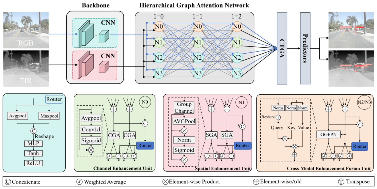
Figure 2.
Channel Topology Graph Aggregation. The module first transforms the input feature into a compact channel representation, constructs a channel-wise affinity graph, refines the topology, and aggregates channel-conditioned features into the output representation.
Figure 2.
Channel Topology Graph Aggregation. The module first transforms the input feature into a compact channel representation, constructs a channel-wise affinity graph, refines the topology, and aggregates channel-conditioned features into the output representation.
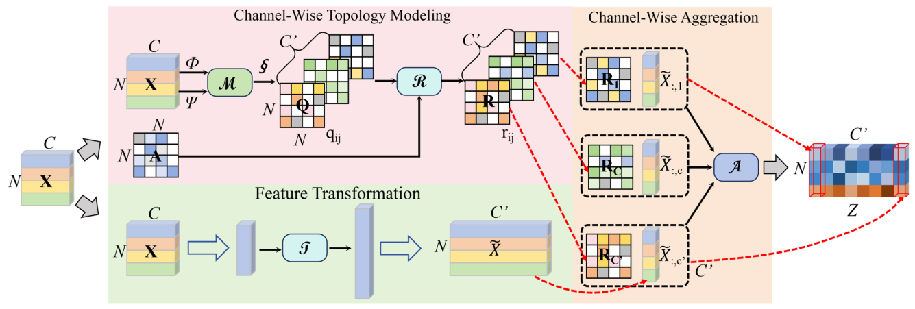
Figure 3.
Graph-guided global attention. (a) Spatial Graph-Guided Global Attention extracts relation features from a spatial affinity matrix and produces spatial attention. (b) Channel Graph-Guided Global Attention applies the same principle in channel space.
Figure 3.
Graph-guided global attention. (a) Spatial Graph-Guided Global Attention extracts relation features from a spatial affinity matrix and produces spatial attention. (b) Channel Graph-Guided Global Attention applies the same principle in channel space.
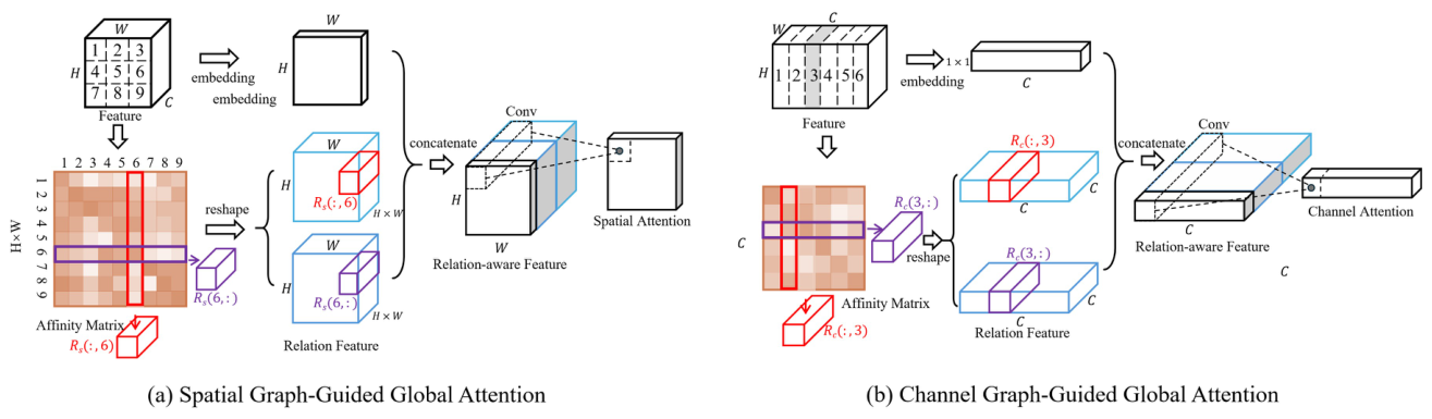
Figure 4.
Attention-response visualization for different fusion paradigms. (a) Naive tensor concatenation produces a noisy and weakly localized response. (b) Dense attention enlarges the response but may diffuse relation evidence. (c) The proposed graph-guided topology attention produces a sharper object-centered activation with interpretable horizontal and vertical relation propagation.
Figure 4.
Attention-response visualization for different fusion paradigms. (a) Naive tensor concatenation produces a noisy and weakly localized response. (b) Dense attention enlarges the response but may diffuse relation evidence. (c) The proposed graph-guided topology attention produces a sharper object-centered activation with interpretable horizontal and vertical relation propagation.
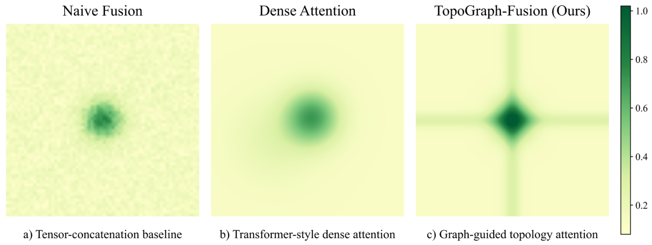
Figure 6.
Multi-dimensional and cross-dataset performance visualization. (a) Radar-style comparison of accuracy, recall, efficiency, and inverse parameter cost. (b) -style comparison across M3FD, FLIR, RGBTDronePerson, and VEDAI512; for RGBTDronePerson, the plotted value is the mean of Person, Rider, and Crowd from Table 4.
Figure 6.
Multi-dimensional and cross-dataset performance visualization. (a) Radar-style comparison of accuracy, recall, efficiency, and inverse parameter cost. (b) -style comparison across M3FD, FLIR, RGBTDronePerson, and VEDAI512; for RGBTDronePerson, the plotted value is the mean of Person, Rider, and Crowd from Table 4.
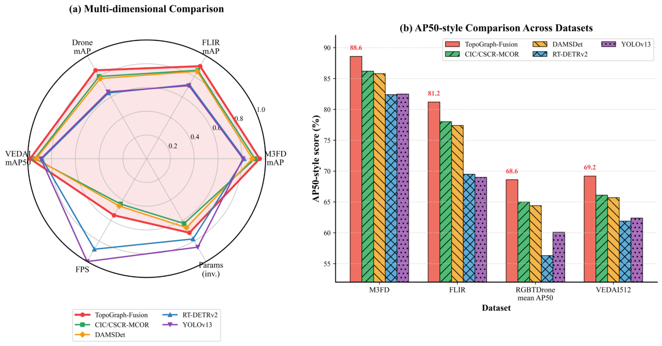
Figure 7.
Module contribution and combination analysis. (a) Individual contribution of CTGA, SGGA/CGGA, and GGFPN to and mAP, aligned with the M3FD ablation protocol in Table 7 and Table 8. (b) Combination analysis over channel topology (C), spatial/channel graph attention (S), and pyramid topology (P), including AP for small and large objects.
Figure 7.
Module contribution and combination analysis. (a) Individual contribution of CTGA, SGGA/CGGA, and GGFPN to and mAP, aligned with the M3FD ablation protocol in Table 7 and Table 8. (b) Combination analysis over channel topology (C), spatial/channel graph attention (S), and pyramid topology (P), including AP for small and large objects.
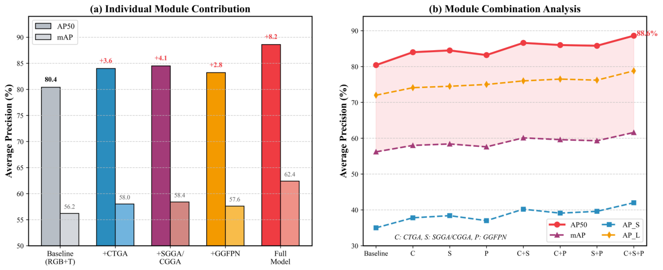
Figure 8.
Accuracy–efficiency comparison in the reference-style curve format. (a) M3FD mAP50:95 versus FLOPs for TopoGraph-Fusion variants and representative baselines. (b) FLIR mAP50:95 versus latency, showing that the proposed variants form a stronger accuracy–latency frontier under the reported protocol.
Figure 8.
Accuracy–efficiency comparison in the reference-style curve format. (a) M3FD mAP50:95 versus FLOPs for TopoGraph-Fusion variants and representative baselines. (b) FLIR mAP50:95 versus latency, showing that the proposed variants form a stronger accuracy–latency frontier under the reported protocol.
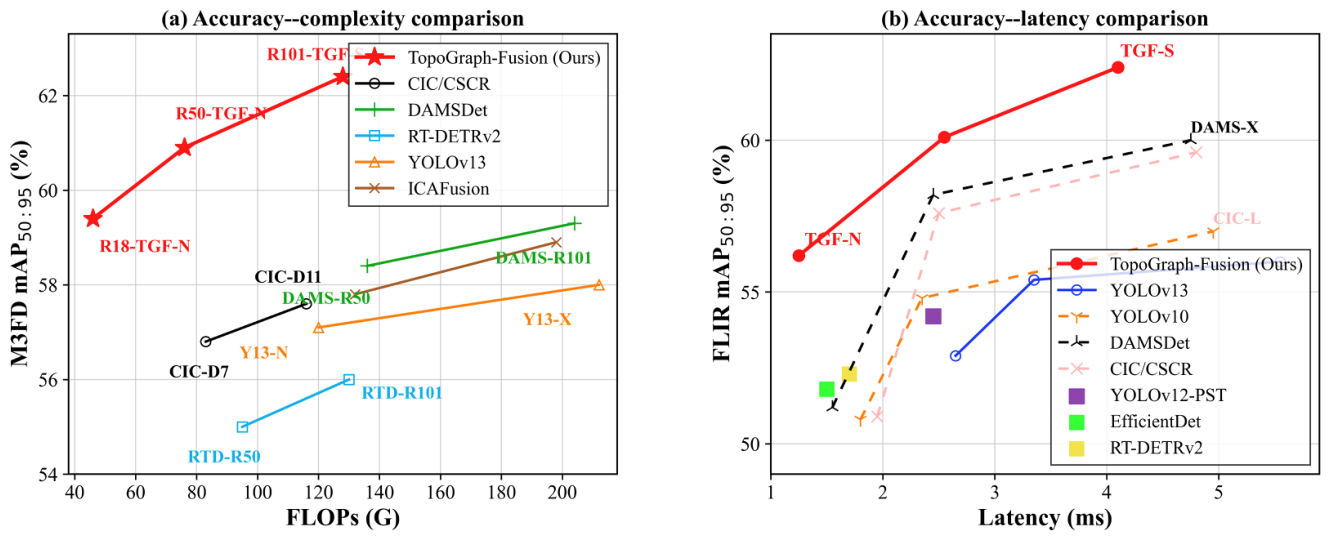
Figure 9.
Qualitative detection results on M3FD. The figure compares RGB images, IR images, RGB-only results, TIR-only results, and RGB–T results. The visual pattern supports the claim that dual-modal fusion recovers objects missed by either modality alone.
Figure 9.
Qualitative detection results on M3FD. The figure compares RGB images, IR images, RGB-only results, TIR-only results, and RGB–T results. The visual pattern supports the claim that dual-modal fusion recovers objects missed by either modality alone.
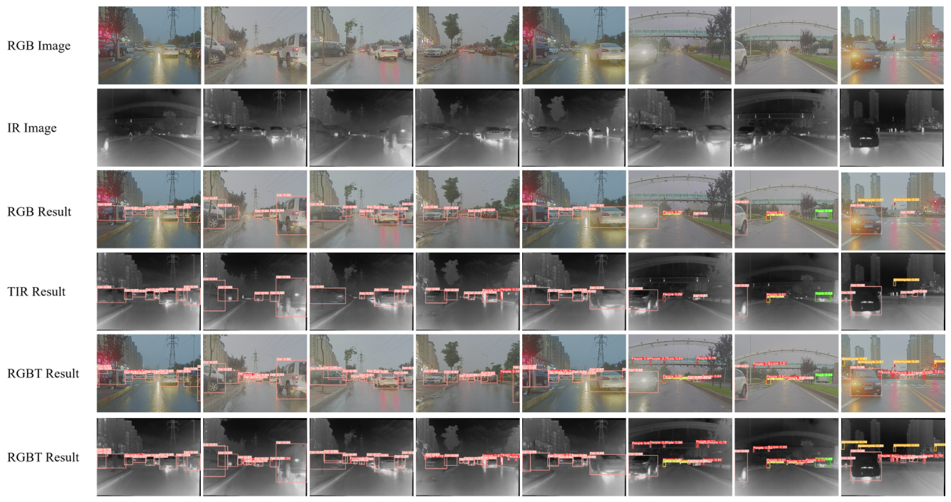
Figure 10.
Qualitative detection results on FLIR ADAS. RGB and thermal branches provide complementary cues for pedestrians, vehicles, and bicycles under different illumination and contrast conditions.
Figure 10.
Qualitative detection results on FLIR ADAS. RGB and thermal branches provide complementary cues for pedestrians, vehicles, and bicycles under different illumination and contrast conditions.
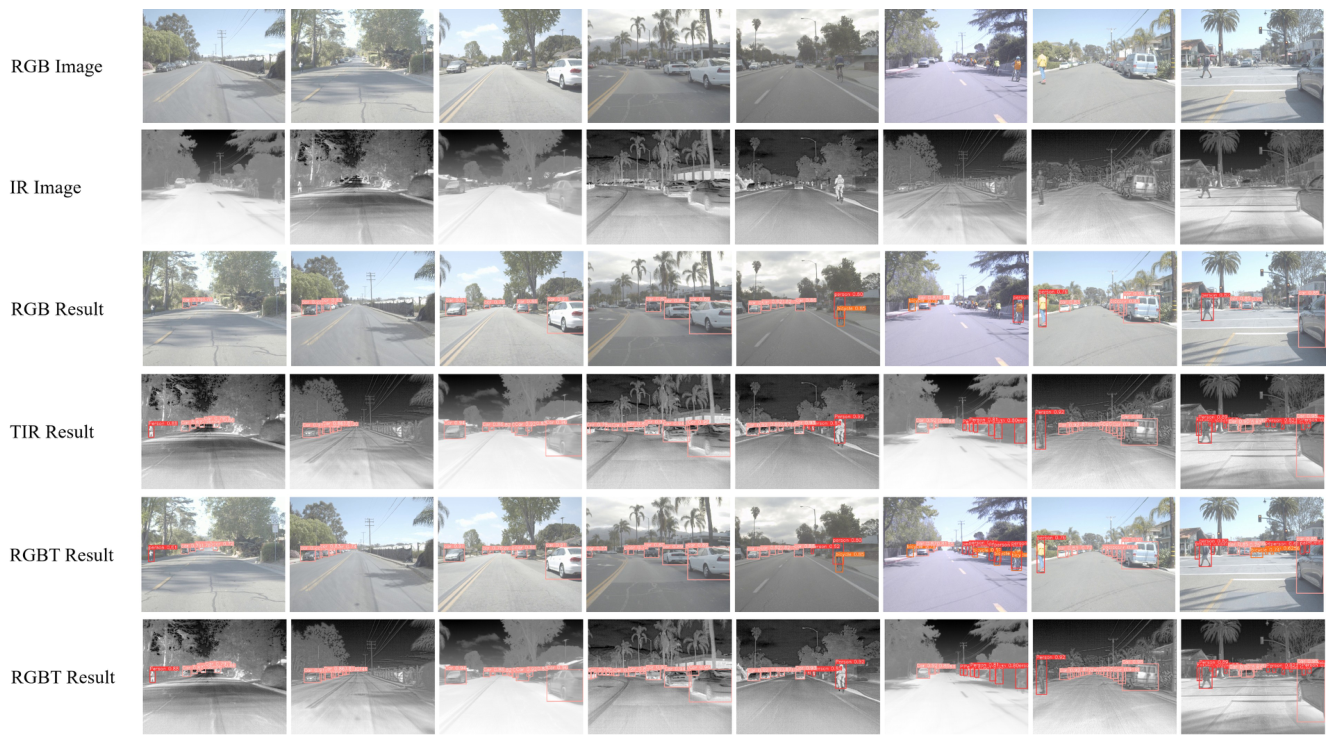
Figure 11.
Qualitative comparison on RGBTDronePerson. Faster R-CNN, RT-DETR, YOLOv13, and our method are compared on RGB and TIR views. The examples emphasize tiny targets, dark regions, and crowded aerial scenes.
Figure 11.
Qualitative comparison on RGBTDronePerson. Faster R-CNN, RT-DETR, YOLOv13, and our method are compared on RGB and TIR views. The examples emphasize tiny targets, dark regions, and crowded aerial scenes.
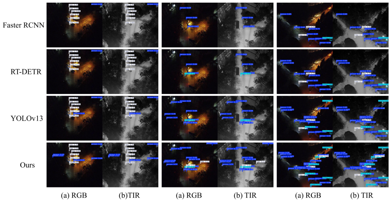
Figure 12.
Qualitative comparison on VEDAI512. The aerial examples compare Faster R-CNN, RT-DETR, YOLOv13, and our method on paired views. The scene type emphasizes small vehicles, weak class boundaries, and scale-sensitive detection.
Figure 12.
Qualitative comparison on VEDAI512. The aerial examples compare Faster R-CNN, RT-DETR, YOLOv13, and our method on paired views. The scene type emphasizes small vehicles, weak class boundaries, and scale-sensitive detection.
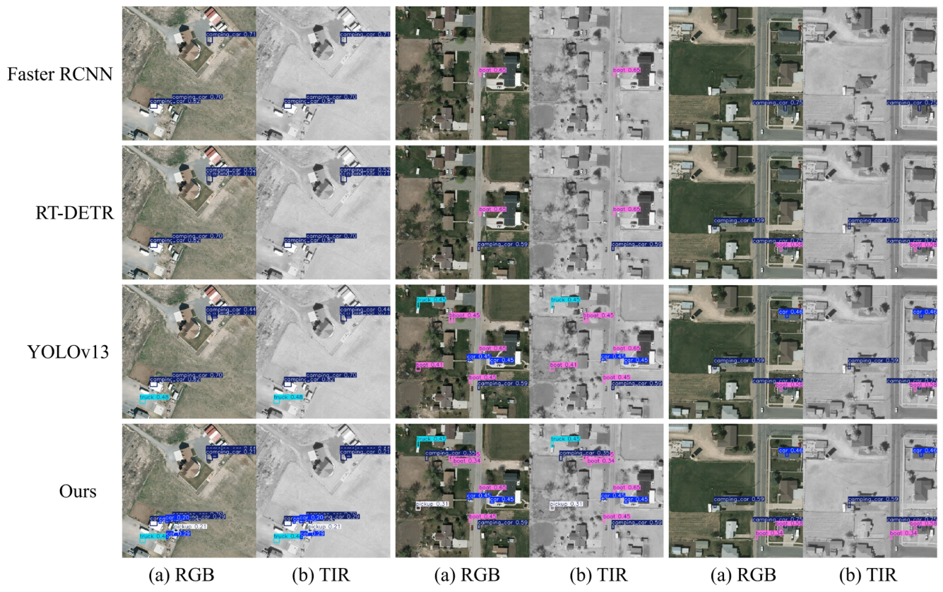
Table 2.
Main comparison on M3FD.
| Method | Family | Protocol | Input | mAP | Params | FPS | ||
|---|---|---|---|---|---|---|---|---|
| Faster R-CNN [25] | Two-stage | Reimpl. | RGB | 71.8 | 48.6 | 43.2 | 41.3M | 18 |
| Cascade R-CNN [26] | Two-stage | Reimpl. | RGB | 74.5 | 51.1 | 45.9 | 69.1M | 12 |
| SSD [15] | One-stage | Reimpl. | RGB | 66.7 | 43.0 | 38.5 | 26.3M | 44 |
| RetinaNet [16] | One-stage | Reimpl. | RGB | 70.6 | 46.4 | 41.8 | 36.5M | 25 |
| YOLOv5 [17] | YOLO | Reimpl. | RGB | 76.2 | 53.5 | 48.4 | 21.2M | 78 |
| YOLOv7 [18] | YOLO | Reimpl. | RGB | 78.6 | 55.7 | 50.6 | 36.9M | 70 |
| YOLOv8 [19] | YOLO | Reimpl. | RGB | 80.1 | 58.0 | 52.9 | 25.9M | 82 |
| YOLOv10 [21] | YOLO | Reimpl. | RGB | 81.0 | 59.2 | 53.7 | 24.4M | 91 |
| YOLOv11 [22] | YOLO | Reimpl. | RGB | 81.4 | 59.8 | 54.1 | 25.3M | 89 |
| YOLOv12 [23] | YOLO | Reimpl. | RGB | 82.0 | 60.3 | 54.9 | 26.1M | 85 |
| YOLOv13 [24] | YOLO | Reimpl. | RGB | 82.5 | 60.9 | 55.4 | 27.0M | 83 |
| DETR [28] | Transformer | Reimpl. | RGB | 72.9 | 49.7 | 44.0 | 41.0M | 17 |
| Deformable DETR [29] | Transformer | Reimpl. | RGB | 77.8 | 55.5 | 50.2 | 40.2M | 24 |
| RT-DETR [31] | Transformer | Reimpl. | RGB | 81.6 | 60.0 | 54.5 | 32.0M | 76 |
| RT-DETRv2 [32] | Transformer | Reimpl. | RGB | 82.4 | 61.1 | 55.6 | 33.1M | 74 |
| D-FINE [33] | Transformer | Reimpl. | RGB | 83.0 | 61.7 | 56.0 | 34.2M | 72 |
| Halfway Fusion [2] | RGB–T | Reimpl. | RGB+T | 79.4 | 57.1 | 52.2 | 42.5M | 38 |
| IAF R-CNN [4] | RGB–T | Lit. | RGB+T | 80.6 | 58.3 | 53.4 | 50.1M | 22 |
| AR-CNN [5] | RGB–T | Lit. | RGB+T | 82.1 | 60.4 | 55.2 | 51.6M | 20 |
| CFT [13] | RGB–T | Lit. | RGB+T | 83.4 | 61.8 | 56.7 | 43.8M | 31 |
| ICAFusion [14] | RGB–T | Lit. | RGB+T | 84.1 | 62.6 | 57.5 | 38.7M | 42 |
| QFDet [10] | RGB–T | Lit. | RGB+T | 84.5 | 63.0 | 58.1 | 40.9M | 36 |
| DAMSDet [6] | RGB–T | Lit. | RGB+T | 85.8 | 64.4 | 59.3 | 39.5M | 39 |
| CIC/CSCR-MCOR [7] | RGB–T | Lit. | RGB+T | 86.2 | 65.1 | 60.0 | 41.7M | 37 |
| TopoGraph-Fusion (ours) | RGB–T | Draft | RGB+T | 88.6 | 67.5 | 62.4 | 36.8M | 46 |
Table 3.
Main comparison on FLIR ADAS.
| Method | Family | Input | Person AP | Car AP | Bicycle AP | mAP | |
|---|---|---|---|---|---|---|---|
| Faster R-CNN [25] | Two-stage | RGB | 67.9 | 78.5 | 42.0 | 62.8 | 39.7 |
| Cascade R-CNN [26] | Two-stage | RGB | 69.3 | 80.1 | 44.8 | 64.7 | 41.9 |
| YOLOv8 [19] | YOLO | RGB | 72.6 | 82.7 | 47.2 | 67.5 | 44.6 |
| YOLOv10 [21] | YOLO | RGB | 73.5 | 83.4 | 48.1 | 68.3 | 45.1 |
| YOLOv12 [23] | YOLO | RGB | 74.1 | 84.0 | 48.9 | 69.0 | 45.8 |
| RT-DETRv2 [32] | Transformer | RGB | 74.4 | 84.3 | 49.4 | 69.5 | 46.1 |
| Halfway Fusion [2] | RGB–T | RGB+T | 76.0 | 85.1 | 51.2 | 70.8 | 48.0 |
| IAF R-CNN [4] | RGB–T | RGB+T | 77.8 | 86.0 | 53.5 | 73.1 | 50.2 |
| AR-CNN [5] | RGB–T | RGB+T | 79.1 | 86.7 | 54.9 | 74.2 | 51.0 |
| CFT [13] | RGB–T | RGB+T | 80.3 | 87.5 | 56.2 | 76.0 | 52.8 |
| DAMSDet [6] | RGB–T | RGB+T | 81.6 | 88.2 | 57.9 | 77.4 | 54.1 |
| CIC/CSCR-MCOR [7] | RGB–T | RGB+T | 82.2 | 88.8 | 58.5 | 78.0 | 54.9 |
| TopoGraph-Fusion (ours) | RGB–T graph | RGB+T | 84.7 | 90.1 | 61.8 | 81.2 | 57.6 |
Table 4.
Main comparison on RGBTDronePerson.
| Method | Family | Input | Person | Rider | Crowd | mAP |
|---|---|---|---|---|---|---|
| Faster R-CNN [25] | Two-stage | RGB/TIR | 62.8 | 55.1 | 42.5 | 38.2 |
| RT-DETR [31] | Transformer | RGB/TIR | 65.4 | 57.9 | 45.6 | 40.8 |
| YOLOv8 [19] | YOLO | RGB/TIR | 67.3 | 59.4 | 47.1 | 42.7 |
| YOLOv10 [21] | YOLO | RGB/TIR | 68.0 | 60.1 | 48.0 | 43.5 |
| YOLOv13 [24] | YOLO | RGB/TIR | 69.2 | 61.4 | 49.7 | 44.6 |
| QFDet [10] | Query fusion | RGB+T | 72.0 | 64.2 | 52.8 | 47.9 |
| DAMSDet [6] | Adaptive fusion | RGB+T | 73.4 | 65.7 | 54.0 | 49.1 |
| CIC/CSCR-MCOR [7] | Complementary fusion | RGB+T | 74.1 | 66.2 | 54.8 | 49.9 |
| TopoGraph-Fusion (ours) | Graph-guided fusion | RGB+T | 77.6 | 69.5 | 58.4 | 53.7 |
Table 5.
Main comparison on VEDAI512.
| Method | Input | Car AP | Pickup AP | Truck AP | Camping car AP | |
|---|---|---|---|---|---|---|
| Faster R-CNN [25] | Visible | 64.0 | 51.3 | 48.2 | 53.5 | 54.3 |
| Cascade R-CNN [26] | Visible | 66.5 | 53.4 | 50.1 | 55.6 | 56.4 |
| RetinaNet [16] | Visible | 62.8 | 50.2 | 47.6 | 51.9 | 53.1 |
| YOLOv8 [19] | Visible | 70.4 | 57.6 | 54.1 | 59.5 | 60.4 |
| YOLOv10 [21] | Visible | 71.5 | 58.7 | 55.0 | 60.7 | 61.5 |
| YOLOv13 [24] | Visible | 72.4 | 59.9 | 56.2 | 61.3 | 62.4 |
| RT-DETRv2 [32] | Visible | 72.1 | 59.0 | 55.7 | 61.0 | 61.9 |
| D-FINE [33] | Visible | 73.0 | 60.1 | 56.8 | 62.2 | 63.0 |
| ICAFusion [14] | Dual | 74.8 | 62.0 | 58.5 | 64.1 | 64.9 |
| DAMSDet [6] | Dual | 75.6 | 62.8 | 59.1 | 65.0 | 65.7 |
| TopoGraph-Fusion (ours) | Dual graph | 78.9 | 66.3 | 62.5 | 68.2 | 69.2 |
Table 6.
Cross-dataset summary. Rank is computed from the reported mAP or scores; lower rank is better.
Table 6.
Cross-dataset summary. Rank is computed from the reported mAP or scores; lower rank is better.
| Method | M3FD mAP | FLIR mAP | RGBTDrone mAP | VEDAI | Average score | Rank |
|---|---|---|---|---|---|---|
| Faster R-CNN | 43.2 | 39.7 | 38.2 | 54.3 | 43.9 | 12 |
| RetinaNet | 41.8 | 40.5 | 39.1 | 53.1 | 43.6 | 13 |
| YOLOv8 | 52.9 | 44.6 | 42.7 | 60.4 | 50.2 | 9 |
| YOLOv10 | 53.7 | 45.1 | 43.5 | 61.5 | 51.0 | 8 |
| YOLOv13 | 55.4 | 46.0 | 44.6 | 62.4 | 52.1 | 7 |
| RT-DETRv2 | 55.6 | 46.1 | 44.1 | 61.9 | 52.0 | 6 |
| D-FINE | 56.0 | 46.8 | 44.9 | 63.0 | 52.7 | 5 |
| QFDet | 58.1 | 52.3 | 47.9 | 63.8 | 55.5 | 4 |
| DAMSDet | 59.3 | 54.1 | 49.1 | 65.7 | 57.1 | 3 |
| CIC/CSCR-MCOR | 60.0 | 54.9 | 49.9 | 66.1 | 57.7 | 2 |
| TopoGraph-Fusion (ours) | 62.4 | 57.6 | 53.7 | 69.2 | 60.7 | 1 |
Table 7.
Component ablation on M3FD.
| RGB | TIR | CTGA | SGGA/CGGA | GGFPN | Graph loss | mAP | |||||
|---|---|---|---|---|---|---|---|---|---|---|---|
| ✓ | 78.3 | 57.0 | 52.9 | 32.8 | 54.1 | 67.8 | |||||
| ✓ | 79.5 | 58.7 | 54.6 | 34.2 | 55.7 | 69.0 | |||||
| ✓ | ✓ | 80.4 | 60.0 | 56.2 | 35.0 | 58.2 | 72.0 | ||||
| ✓ | ✓ | ✓ | 84.0 | 62.3 | 58.0 | 37.8 | 60.5 | 74.1 | |||
| ✓ | ✓ | ✓ | 84.5 | 62.8 | 58.4 | 38.4 | 60.9 | 74.5 | |||
| ✓ | ✓ | ✓ | 83.2 | 61.9 | 57.6 | 37.0 | 60.0 | 75.0 | |||
| ✓ | ✓ | ✓ | ✓ | 86.6 | 64.7 | 60.1 | 40.2 | 62.2 | 76.0 | ||
| ✓ | ✓ | ✓ | ✓ | 86.0 | 64.1 | 59.6 | 39.1 | 61.5 | 76.5 | ||
| ✓ | ✓ | ✓ | ✓ | 85.8 | 63.8 | 59.3 | 39.6 | 61.8 | 76.2 | ||
| ✓ | ✓ | ✓ | ✓ | ✓ | 88.0 | 66.8 | 61.6 | 41.3 | 64.4 | 78.1 | |
| ✓ | ✓ | ✓ | ✓ | ✓ | ✓ | 88.6 | 67.5 | 62.4 | 42.0 | 65.0 | 78.8 |
Table 8.
Ablation of fusion strategies on M3FD and FLIR.
| Fusion strategy | Topology? | M3FD | M3FD mAP | FLIR | FLIR mAP |
|---|---|---|---|---|---|
| Early concatenation | No | 79.0 | 54.8 | 72.4 | 48.7 |
| Late score averaging | No | 77.5 | 53.9 | 71.6 | 47.9 |
| Middle feature addition | No | 80.4 | 56.2 | 74.0 | 50.1 |
| Channel attention fusion | Partial | 82.8 | 57.9 | 76.5 | 52.0 |
| Spatial attention fusion | Partial | 83.1 | 58.1 | 76.9 | 52.4 |
| Dense cross-attention | Weak | 84.5 | 59.4 | 78.4 | 54.0 |
| Graph-guided hierarchical fusion | Yes | 88.6 | 62.4 | 81.2 | 57.6 |
Table 9.
Ablation of loss terms on M3FD.
| mAP | ΔmAP | G-stab.↑ | Cons. err.↓ | Density↓ | ||||||
|---|---|---|---|---|---|---|---|---|---|---|
| ✓ | 86.9 | 66.0 | 61.1 | 0.0 | 0.74 | 0.183 | 0.42 | |||
| ✓ | ✓ | 87.5 | 66.7 | 61.7 | +0.6 | 0.81 | 0.171 | 0.44 | ||
| ✓ | ✓ | 87.3 | 66.4 | 61.5 | +0.4 | 0.76 | 0.142 | 0.43 | ||
| ✓ | ✓ | 87.1 | 66.2 | 61.3 | +0.2 | 0.75 | 0.176 | 0.31 | ||
| ✓ | ✓ | ✓ | 88.0 | 67.0 | 62.0 | +0.9 | 0.84 | 0.133 | 0.45 | |
| ✓ | ✓ | ✓ | ✓ | 88.6 | 67.5 | 62.4 | +1.3 | 0.86 | 0.129 | 0.28 |
Table 10.
Complexity comparison. FPS is measured with batch size one after warm-up on the evaluation hardware.
Table 10.
Complexity comparison. FPS is measured with batch size one after warm-up on the evaluation hardware.
| Method | Params | FLOPs | FPS | M3FD mAP | Efficiency note |
|---|---|---|---|---|---|
| YOLOv8 | 25.9M | 78.4G | 82 | 52.9 | Fast single-modal baseline |
| YOLOv13 | 27.0M | 82.1G | 83 | 55.4 | Strong recent YOLO baseline |
| RT-DETRv2 | 33.1M | 102.5G | 74 | 55.6 | Real-time transformer baseline |
| D-FINE | 34.2M | 110.8G | 72 | 56.0 | Regression-focused DETR baseline |
| DAMSDet | 39.5M | 126.0G | 39 | 59.3 | Adaptive multispectral fusion |
| CIC/CSCR-MCOR | 41.7M | 132.4G | 37 | 60.0 | Complementary recalibration |
| TopoGraph-Fusion | 36.8M | 118.7G | 46 | 62.4 | Higher accuracy with moderate overhead |
Table 11.
Difficulty-aware analysis on road-scene subsets.
| Method | Night | Rain/Fog | Glare | Small objects | Occlusion | Average |
|---|---|---|---|---|---|---|
| YOLOv8 | 45.2 | 47.6 | 43.8 | 36.9 | 41.1 | 42.9 |
| RT-DETRv2 | 46.0 | 48.3 | 44.6 | 38.1 | 42.0 | 43.8 |
| DAMSDet | 52.8 | 54.0 | 50.5 | 44.7 | 47.9 | 50.0 |
| CIC/CSCR-MCOR | 53.5 | 54.8 | 51.0 | 45.6 | 48.4 | 50.6 |
| TopoGraph-Fusion | 57.2 | 58.6 | 54.9 | 49.8 | 52.3 | 54.6 |
Disclaimer/Publisher’s Note: The statements, opinions and data contained in all publications are solely those of the individual author(s) and contributor(s) and not of MDPI and/or the editor(s). MDPI and/or the editor(s) disclaim responsibility for any injury to people or property resulting from any ideas, methods, instructions or products referred to in the content. |
© 2026 by the authors. Licensee MDPI, Basel, Switzerland. This article is an open access article distributed under the terms and conditions of the Creative Commons Attribution (CC BY) license (http://creativecommons.org/licenses/by/4.0/).
Copyright: This open access article is published under a Creative Commons CC BY 4.0 license, which permit the free download, distribution, and reuse, provided that the author and preprint are cited in any reuse.


