
Submitted:
24 June 2026
Posted:
24 June 2026
You are already at the latest version
Abstract
One of the defining challenges of our time is the management of urban traffic. As cities grow denser and more complex, the limitations of traditional fixed-time signal systems become increasingly difficult to ignore. This paper explores how Reinforcement Learning (RL) can offer a smarter and more adaptive alternative for traffic signal control (TSC), showing its potential to optimize traffic flow and reduce congestion. To investigate this potential, we relied on computer simulations as a training and evaluation environment. The results show that RL-based controllers have good adaptive abilities and work better than traditional traffic signal strategies. However, there are still critical challenges, such as scalability to large networks, non-stationarity of the environment, and enforcement of safety constraints that are key barriers to real-world deployment. These findings highlight the significant promise of RL for future traffic management, but also stress the need for further research on robustness, reliability and generalizability of these systems.
Keywords:
reinforcement learning
; deep reinforcement learning
; optimization
; control optimal
; traffic signal control
1. Introduction
Urban traffic congestion has become a critical challenge in modern cities due to the rapid increase in vehicle ownership and the limitations of existing infrastructure. Inefficient traffic signal control (TSC) systems contribute significantly to increased travel time, fuel consumption, and environmental pollution. Traditional traffic signal control strategies, such as fixed-time or actuated control, are often unable to adapt effectively to dynamic and stochastic traffic conditions.
In recent years, reinforcement learning (RL) has emerged as a promising approach for intelligent traffic signal control [3,4]. By modeling the traffic environment as a sequential decision-making problem, RL focuses on sequential decision-making problems, where an agent learns optimal behaviors through trial-and-error interactions with its environment. This paradigm allows for adaptive and data-driven optimization of signal timings, improving overall traffic flow and reducing congestion.
Several classical RL algorithms have been applied to TSC, including Q-learning, SARSA, and Monte Carlo methods. Q-learning, an off-policy algorithm, is known for its fast convergence and ability to approximate optimal policies. However, it may suffer from instability due to overestimation of action values. On the other hand, SARSA, an on-policy method, provides more stable learning but often converges more slowly. Monte Carlo methods, which rely on episodic returns, offer unbiased value estimation but typically exhibit high variance and require longer training periods.
Despite their individual strengths, these algorithms also present inherent limitations when applied independently to complex and dynamic traffic environments. This motivates the need for hybrid approaches that can leverage the advantages of multiple learning strategies while mitigating their weaknesses.
In this paper, we perform a simulation of an intelligent traffic signal control system based on a hybrid reinforcement learning framework. The proposed approach combines Q- learning, SARSA, and Monte Carlo methods into a unified update mechanism, aiming to achieve a balance between convergence speed, stability, and long-term performance. The traffic environment is modeled as a stochastic intersection with dynamic vehicle arrivals, where the RL agent controls the traffic light phases. The performance of the proposed hybrid method is evaluated against classical RL algorithms using key traffic metrics such as average delay, waiting time, throughput, and queue length[12].
The main contributions of this work can be summarized as follows:
- A hybrid RL approach that integrates Q-learning, SARSA, and Monte Carlo updates into a single framework.
- A simulation-based traffic signal control model using a dynamic and stochastic environment.
- A comprehensive performance evaluation using multiple traffic efficiency metrics.
- A comparative analysis demonstrating the effectiveness of the proposed method over classical RL approaches.
2. Background and Preliminaries
In this section, we introduce the essential notions and theoretical background of RL used in this paper [1]. To provide a rigorous foundation for the proposed framework, we present the key mathematical definitions, including the formal representation of the environment, state space, action space, and reward function.
2.1. Reinforcement Learning
RL is a machine learning technique that enables optimal solutions to sequential decision problems through trial and error. It’s a process where an agent (controller) optimizes its behavior by interacting with its uncertain environment. The agent makes decisions and takes actions, and the environment provides feedback, facilitating state changes. The goal is to learn the optimal behavior in an environment to maximize the reward.
The RL process begins with the agent observing the current state of the environment, selecting an action, receiving a reward from the environment, adjusting its policy, and repeating the cycle. The agent and the environment interact at discrete time steps , where the agent observes the state at time step t, denoted by , produces an action , receives a reward , and transitions to a new state . This interaction is further illustrated in Figure 1.
The agent aims to learn a policy to maximize total cumulative reward over time. Unlike unsupervised learning, which seeks hidden structures in unlabeled data without focusing on rewards. Thus, RL is the third ML paradigm. Along with supervised and unsupervised learning, dedicated to maximizing an agent’s total rewards from its environment.Formally, RL problems can be formulated in the framework of Markovian Decision Process (MDPs).
2.2. MDP: Markov Decision Process
In this section, we present the fundamental principles of Markov Decision Processes (MDPs), a mathematical framework for modeling sequential decision-making problems commonly encountered in RL.
A MDP consists of five elements as follows where :
- is the space of environmental states.
- is the space of actions the agent can take.
- P is a transition function (the probability of ending in state , given that action a is taken in state s.can be represented by a conditional probability mass function denoted by ).
- : The reward function: provides the expected reward conditioned on being in a specific state s and taking a particular action a.
- is a discount factor that specifies how much immediate rewards are favored over future rewards., When is equal to 1, it indicates that future rewards are considered as important as present rewards. Conversely, when is equal to 0, it means that only present rewards are valued.
Through interactions with the environment, the agent generates a trajectory , consisting of a sequence . At the end of a trajectory, our agent will have accumulated a sum of rewards what we refer to as the return. The overall goal of the agent is to maximize the cumulative reward along a trajectory up to time t by choosing the actions obtained along this trajectory . Note that when () is finite, it is referred to as a finite episode, whereas if T is infinite, it is referred to as a continuing episode ( ).
2.3. Policies and value function
We define a policy as a function that assigns a probability distribution over the action space for each state. If there is only one action associated with each state, it is called a deterministic policy. In the general case, denotes the probability of choosing action in state .
The ultimate goal of RL is to find the optimal policy that maximizes the expected cumulative discounted reward, formally defined as:
the agent seeks to learn a behavior that not only reacts greedily to immediate feedback but also anticipates long-term consequences term.
To evaluate an agent’s performance from a specific initial state under a particular policy, we use a metric called the value function. This function measures the quality of a state by estimating the total rewards expected from the trajectory. It indicates how beneficial it is to be in a certain state. Most RL algorithms estimate a value function , which is always associated with a policy , as the expected rewards depend on the actions taken. The state-value function is denoted as follows:
In RL, the value function applies to all policies, and when the policy is optimal, it is referred to as theoptimal value function. Additionally, we define the Q-value function, which represents the value of starting from a state s, taking an action a, then following policy until reaching a terminal state. The action-value function is denoted:
A fundamental property of the value function is its satisfaction of the following recursive relationship:
This relationship is called the Bellman equation for (a similar form can be derived for the Q-function).
These 3 concepts: policy, state-value function and action-value function are the foundation of all RL algorithms we will discuss. Solving a RL problem involves finding a policy that achieves high long-term rewards.
The value function provides a partial ordering over policies, allowing us to determine whether one policy is better than or equal to another policy .
If a policy is better than or equal to all other policies, it is referred to as the optimal policy. The optimal policy is denoted as .
Given that the optimal action-value function is the one which gives the maximum expected return, the optimal policy can be found by choosing the action that gives the maximum Q-value for the given state s:
The optimal Q-function follows the Bellman equation and it can be learned through an iterative update process:
where is the learning rate, and is the temporal difference (TD) error:
We denote as the TD-target.
3. Traffic Signal Control Problem
Traditional Traffic Signal Control (TSC) approaches are rooted in classical traffic flow theory and have long served as the backbone of urban traffic management [8]. However, these methods do not respond well to real-time traffic changes. The max-pressure method tries to reduce congestion by balancing traffic between lanes, but it assumes that the roads after the intersection have unlimited space, which is not realistic. Overall, these methods cannot adapt well to changing traffic conditions and limit their effectiveness in real-world deployment scenarios.
3.1. TSC Types
TSC frameworks play an essential role in managing urban mobility, safety improvement, and optimizing intersection efficiency.These approaches can generally be divided into three main categories: fixed-time (pre timed) control, actuated control and adaptive control, each of which has several variants. This Figure 2 presents the main categories of traffic signal control methods and their common subtypes. trees, positioning
3.2. Reinforcement Learning for TSC
In RL-based traffic signal control, the decision-making process relies on several key components that interact dynamically to optimize traffic flow. The overall functioning of RLin a traffic signal control system can be explained by the following main steps.
- Environment: The traffic network constitutes the environment in which the RL agent operates. It may include intersections, vehicle and pedestrian flows, and external disturbances like weather or sudden congestion. The RL agent does not directly control this environment but learns to react to its dynamics by optimizing signal timings (Figure 3).
- RL Agent: The RL agent is the brain of the system, it receives the incoming traffic data and decides the best signal phases. It learns to minimize congestion, delays and emissions through continuous interaction with the environment depending on the method used.
- Action: Traffic light control systems offer options such as timing adjustment and synchronized green light lane design choices. Once an action is selected, the system performs signal adjustments (e.g. green time extension, phase skipping, cycle length adjustment, coordination of multiple intersections) as per the agent output.
- Environment Update: After applying the control decisions, the environment evolves. Vehicles move, congestion shifts, and new traffic enters, resulting in a new state that becomes the input for the agent’s next decision.
- Reward Calculation: The system evaluates the agent’s decision using predefined metrics. Common reward functions are reduction in waiting time, queue lengths, fuel consumption, emissions, and enhancement of pedestrian safety and traffic balance.
- Reward Signal Feedback: The computed reward is fed back into the RL algorithm, refining its policy. Through this iterative process, the agent improves its control strategy, enabling real-time, adaptive signal management.
3.3. RL Algorithms for Traffic Signal Control
There are three main types of RL algorithms for traffic control: value-based, policy-based and actor-critic methods. Each of them has a different mechanism to optimize the traffic performance.
3.3.1. Value-Based Algorithms
This RL type uses a value function to estimate expected returns of actions in specific traffic states, selecting actions to maximize expected rewards. It has proven effective for discrete tasks like phase selection and green-time allocation, although scalability can be problematic in larger or continuous action spaces. Common examples include Q-learning (QL) and deep Q-networks (DQNs).
-
Q-Learning: An off-policy algorithm that iteratively updates an action-value function independently of the current policy. Suitable for single-intersection control, it learns state-action values via:Q is efficient in discrete environments but struggles with high-dimensional networks.
- Deep Q-Networks: DQN enhances Q-learning by approximating the Q-function with deep neural networks (NN). Techniques such as experience replay and target networks improve training stability, enabling coordination across multiple intersections. The update rule is given by:
3.3.2. Policy-Based Algorithms
This algorithm optimizes policy directly, bypassing value estimation, making it suitable for continuous action spaces and enabling fine-grained control such as dynamic phase timing. It offers flexibility in complex environments but demands precise hyperparameter tuning, with PPO noted for its stability and efficiency.
- Proximal Policy Optimization (PPO) is a RL algorithm that constrains policy updates to maintain training stability. It is commonly employed in multi-intersection control systems and effectively balances exploration and exploitation within large-scale networks. The clipped objective function may be expressed as:where : and denotes the advantage function [9].
3.3.3. Actor-Critic Algorithms
Actor-critic approaches represent a particularly compelling hybrid family within the reinforcement learning landscape, as they seek to combine the strengths of bothvalue-based and policy-based methods. The central idea rests on the cooperation of two distinct components: an actor, responsible for proposingactions given the current state, and a critic, whose role is to assess the quality of those decisions. This duality endows the architecture with enhanced learning stability while preserving sufficient computational efficiency to tackle large-scale traffic control problems. Three representative variants are examined below:
-
Deep Deterministic Policy Gradient: The DDPG was specifically designed for continuous action spaces, making it well-suited to tasks such as the dynamic adjustment of signal phase durations at intersections. Its operation relies on two complementary, iterative updates. Firstly, the critic refines its estimate of the state-action value:Secondly, the actor updates its policy by maximising the gradient of this value:While powerful, DDPG is sensitive to tuning.
- Soft Actor-Critic (SAC): To address this sensitivity, SAC enriches the objective function by incorporating an entropy term. This modification naturally encourages broader exploration of control strategies, thereby improving robustness in potentially non-stationary multi-agent environments. The resulting optimisation objective takes the form:where the coefficient governs the trade-off between exploration and exploitation.
-
Advantage Actor-Critic (A2C): ntroduces yet another perspective through the notion of advantage, which quantifies the extent to which a given action outperforms the average expected return in a given state:By substituting this centred signal for the raw reward in the policy update, A2C reduces gradient estimate variance, yielding more stable learning dynamics:The A2C achieves strong results in real-time adaptive control, particularly in collaborative multi-agent architectures where variance reduction plays a decisive role in ensuring convergence.
4. Results and Discussion
4.1. Experimental Setup
In our study, we propose an simulation of an intelligent traffic signal control system using a RL framework. The environment models a single intersection with stochastic vehicle arrivals in both horizontal and vertical directions. Four learning strategies are evaluated: Q-learning, SARSA, Monte Carlo (MC), and the proposed hybrid Method.
Each algorithm is trained over multiple episodes, and its performance is evaluated using key traffic metrics. Including average delay, waiting time, throughput, queue length, and signal phase durations (green and red times). To enhance readability and reduce noise, the results are smoothed using a moving average, and ariability is represented using standard deviation bands.
4.2. Proposed Method
The proposed hybrid approach draws on the complementary strengths of three well-established RL algorithms: Q-Learning, SARSA, and Monte Carlo, with the goal of achieving what no single method can easily deliver on its own: fast convergence, stable learning behavior, and reliable long-term reward estimation.
Each algorithm contributes a distinct capability. Q-Learning brings strong off-policy learning, enabling the agent to rapidly approximate optimal action values. SARSA, through its on-policy update mechanism, promotes greater stability by avoiding overly aggressive updates in stochastic environments like traffic control. Monte Carlo methods complement both by relying on complete episode returns, which leads to more accurate long-term value estimates.
To integrate these contributions into a coherent learning rule, we define a hybrid Q-value update based on a weighted combination of the three estimators:
where is the learning rate, governing how much weight is given to new information relative to the current estimate. The coefficients , , and control the relative influence of each method and are subject to the normalization constraint:
Rather than fixing these weights throughout training, we introduce an adaptive scheduling strategy that adjusts their values dynamically as learning progresses. Let denote the normalized training progress:
The weights then evolve as time-dependent functions , , and , each reflecting the natural role of its associated method at different stages of training. In the early episodes, dominates to favor the conservative and stable updates of SARSA, which is especially valuable in highly dynamic environments. As training advances, gradually increases, allowing Q-Learning to drive faster convergence toward an optimal policy. In the final stages, becomes predominant, leveraging the improved reliability of complete episode returns for fine-grained value refinement.
At each update step, the weights are renormalized to ensure is always satisfied. This phased, adaptive design allows the agent to benefit from each learning paradigm precisely when it is most effective, resulting in a more robust and well-rounded policy for complex control tasks such as adaptive traffic signal management [2].
4.3. Traffic Performance Evaluation
To evaluate the effectiveness of the proposed traffic control system, several key performance metrics are considered.
- 1.
- The Average Delay measures the mean time vehicles spend waiting before passing through the intersection, reflecting overall congestion levels;
- 2.
- The Throughput represents the number of vehicles successfully processed per unit time, indicating the efficiency of traffic flow;
- 3.
- The Queue Length corresponds to the number of vehicles waiting in each lane or approach, providing insight into spatial congestion dynamics;
- 4.
- The Waiting Time captures the total time each vehicle spends in the system before being served, offering a microscopic view of individual vehicle experience.
Finally, the Reward is defined within the reinforcement learning framework as a scalar feedback signal that encourages desirable behaviors such as minimizing delay and queue buildup while maximizing throughput. Together, these metrics provide a comprehensive evaluation of both system-level efficiency and agent-level learning performance.
4.4. Results
4.4.1. Learning Curves
The 4 RL algorithms were trained over episodes on the single-intersection TSC environment and evaluated across 6 metrics:cumulative reward, average queue length, vehicle throughput,delay per vehicle, and convergence speed. Results are summarised in Table 1.
As shown in Figure 4a, Q-Learning and SARSA plateau early at final rewards, reflecting the bias inherent in single-step bootstrapping under stochastic traffic arrivals. Monte Carlo achieves the highest reward () through unbiased full-return estimates, but at the cost of elevated training variance and reduced throughput ( veh/ep), as high-variance policy updates compromise real-time phase-switching decisions (Figure 4c).
The proposed hybrid method attains a final reward of, a 7.2% improvement over both TD baselines, while achieving the highest throughput among all evaluated algorithms ( veh/ep, veh/ep over Monte Carlo).
In terms of delay, the Hybrid reduces waiting time by relative to Q-Learning and SARSA, with only a gap compared to Monte Carlo (Figure 4d). This trade-off of marginal increase in delay for significant gain in throughput is particularly advantageous in high volume intersection management where the primary operational aim is to maximise the flow of vehicles.
The convergence profiles (Figure 4f) confirm that while the Hybrid converges at episode 2938, it reaches a higher normalised reward ceiling than Q-Learning and SARSA, consistent with the established bias–variance trade-off in RL [2,10].
These results support the adaptive 3-component weighting strategy of the hybrid algorithm. The hybrid starts with Q-Learning (early exploration) as the dominant update signal and smoothly transitions to Sarsa (stable mid-training updates) and eventually Monte Carlo (accurate long-horizon returns). This allows the hybrid to leverage the complementary strengths of the baselines and to overcome their individual shortcomings.
4.4.2. Convergence Analysis
All RL algorithms (Figure 5) improve progressive during training, though with notable differences in speed and stability. Q-learning converges fast but with early fluctuations, SARSA learns more smoothly but slower, and Monte Carlo suffers from high variance due to its episodic nature. The proposed hybrid approach outperforms all three by combining fast convergence with greater stability, confirming the benefit of integrating multiple learning paradigms.
4.5. Comparative Analysis of RL Algorithms
Table 2 summarizes the performance of four RL algorithms (Q-Learning, SARSA, Monte Carlo and a hybrid approach) evaluated for intersection signal control across five metrics. All four methods converged around episode 10 000, indicating similar learning horizons.
In terms of stability, measured by standard deviation of waiting time (Figure 6c), Hybrid exhibited the most stable behavior ( s), while Monte Carlo and the Q-Learningmethod exhibited more variability ( s and s respectively). SARSA was in between
All algorithms perform relatively similar in throughput which shows a slight trade-off between delay minimization and overall flow efficiency. Maximum queue lengths were comparable among the methods, with all algorithms except Hybrid reaching 6 vehicles, while Hybrid reached only 5 vehicles.Figure 6d and Figure 6a further illustrate these differences over the course of training. The throughput curves (Figure 6d) confirm that all methods stabilize at similar levels, while the waiting time and queue length plots (Figure 6c and Figure 6b) highlight the lower variance achieved by Q-Learning. The delay comparison (Figure 6a) corroborates the tabulated values, showing Hybrid consistently producing the shortest delays after convergence.
5. Discussion
The results show that the use of multiple RL techniques results in better performance under dynamic traffic conditions. The hybrid method takes advantage of complementary strengths of:
- Q-learning: fast convergence,
- SARSA: stability,
- Monte Carlo: long-term return estimation.
This combination enhances robustness and adaptability, making the hybrid approach suitable for intelligent TSC.
Overall, the hybrid RL approach outperforms classical methods in each of the metrics assessed. It offers a promising solution for adaptive TSC in stochastic and dynamic environments.
- Average Delay: The hybrid method achieves the lowest average delay among all evaluated algorithms. This indicates its superior capability in minimizing congestion and optimizing traffic signal timing. Q-learning performs competitively but may occasionally lead to suboptimal decisions due to value overestimation.
- Throughput: The throughput results indicate that the hybrid approach allows a higher number of vehicles to pass through the intersection. This reflects a more efficient allocation of green signal phases. SARSA also provides consistent throughput but remains slightly less efficient than the hybrid method.
- Queue Length: Queue length is a key indicator of congestion levels. The hybrid method maintains shorter and more stable queue lengths compared to other approaches. Monte Carlo exhibits higher variability, resulting in fluctuating queue sizes.
- Waiting Time: The total waiting time is significantly reduced using the hybrid approach. This improvement highlights the ability of the proposed method to dynamically adapt signal control decisions based on real-time traffic conditions.
However, this study is limited to one intersection and a discrete state representation. Future work can extend this framework to multi-intersection networks and integrate deep reinforcement learning techniques to handle more complex and high-dimensional environments.
6. Conclusion
This paper presented a comparative study of 4 RL algorithms: Q-Learning, SARSA, Monte Carlo, and a Hybrid approach, applied to adaptive traffic signal control at an isolated intersection. Through extensive simulation over 10,000 training episodes, all methods were evaluated across 5 key performance indicators: average waiting time, waiting time standard deviation, peak queue length, vehicle throughput, and convergence speed. The results confirmed that all four algorithms successfully learned effective signal-switching policies without any prior knowledge of traffic dynamics, validating reinforcement learning as a suitable framework for intelligent intersection management.
From among all tested techniques, the introduced Hybrid algorithm showed uniform and well-balanced results when tested against all measures. Through the use of a phase-based schedule, which incorporates the exploration ability of Monte Carlo, quick convergence capability of Q-Learning, and on-policy stability of SARSA, the introduced hybrid technique can adapt to the dynamic conditions of training as opposed to sticking to a single update strategy. The adaptability of this approach is most relevant in non-stationary environments, such as dynamic real-world traffic situations.
There are many avenues for further investigation including extension of the assessment into multi-intersection networks, incorporation of architectures based on deep RL (e.g., DQN or PPO) for more sophisticated state representation, and use of the framework in simulation environments such as SUMO and VISSIM to test its practical application. The contributions made in this study are significant in providing an alternative and flexible approach to traditional model-free solutions and are thus likely to be considered a valuable starting point for future investigation.
Acknowledgments
“During the preparation of this manuscript, the author(s) used [AI-assisted tools] for the purpose of [grammar checking and language editing]. The authors have reviewed and edited the output and take full responsibility for the content of this publication.”
Abbreviations
The following abbreviations are used in this manuscript:
| RL | Reinforcement learning |
| DRL | Deep Reinforcement learning |
| TSC | Traffic Signal Control |
| MDP | Markov Decision Process |
| PPO | Proximal Policy Optimization |
| MC | Monte carlo |
| 1 | For a more comprehensive introduction to MDPs, please refer to [1]. |
References
- Richard S. Sutton and Andrew G. Barto, Reinforcement Learning: An Introduction; Second Edition. MIT Press, Cambridge, MA, 2018.
- A. Ben Moussa and A. Khazari, Reinforcement Learning for Autonomous Driving: Optimization Strategiesand Methodologies. Artificial Intelligence and Mathematics; Springer Nature Switzerland,2026, 369–385.
- P. Michailidis, I. Michailidis, and E. Kosmatopoulos, Traffic Signal Control via Reinforcement Learning: A Review on Applications and Innovations. Infrastructures 2025, 10, 114,2025. [CrossRef]
- Y. Elbaum, A. Novoselsky and E. Kagan. A Queueing Model for Traffic Flow Control in the Road Intersection, Mathematics 2022, 10(21), 3997. [CrossRef]
- Hashmi, H.T., Ud-Din, S., Khan, M.A., Khan, J.A., Arshad, M., and Hassan, M.U.,“Traffic Flow Optimization at Toll Plaza Using Proactive Deep Learning Strategies,” Infrastructures, Vol. 9, Article 87, pp. 1–18, 2024.
- S. El-Tantawy, B. Abdulhai, and H. Abdelgawad, Multiagent Reinforcement Learning for Integrated Network of Adaptive Traffic Signal Controllers (MARLIN-ATSC): Methodology and Large-Scale Application on Downtown Toronto;IEEE Transactions on Intelligent Transportation Systems, Vol. 14, No. 3, pp. 1140–1150, 2013.
- H. Wei, G. Zheng, H. Yao, and Z. Li, IntelliLight: A Reinforcement Learning Approach for Intelligent Traffic Light Control; In Proceedings of the 24th ACM SIGKDD International Conference on Knowledge Discovery and Data Mining (KDD 2018), London, UK, pp. 2496–2505, 2018.
- N. Rouphail, A. Tarko, and J. Li, Traffic Flow at Signalized Intersections; Federal Highway Administration, Washington, DC, USA, 1992.
- H. Wei, X. Liu, L. Mashayekhy, and K. Decker, Mixed-Autonomy Traffic Control with Proximal Policy Optimization; In Proceedings of the 2019 IEEE Vehicular Networking Conference (VNC), Los Angeles, CA, USA, pp. 1–8, 2019.
- Transportation Research Board, Highway Capacity Manual; National Academy of Sciences, Washington, DC, USA, 2000.
- B. Abdulhai, R. Pringle, and G.J. Karakoulas, Reinforcement Learning for True Adaptive Traffic Signal Control; Journal of Transportation Engineering, Vol. 129, No. 3, pp. 278–285, 2003.
- M. Guo, P. Wang, C.-Y. Chan, and S. Askary, A Reinforcement Learning Approach for Intelligent Traffic Signal Control at Urban Intersections; In Proceedings of the IEEE Intelligent Transportation Systems Conference (ITSC), 2019.
- M. Guo, P. Wang, C.-Y. Chan, and S. Askary, A Reinforcement Learning Approach for Intelligent Traffic Signal Control at Urban Intersections; In Proceedings of the IEEE Intelligent Transportation Systems Conference (ITSC), 2019.
- S.M. Rayhanul Swapno et al., Traffic Light Control Using Reinforcement Learning; In Proceedings of the 2024 International Conference on Integrated Circuits and Communication Systems (ICICACS), pp. 1–7, IEEE, 2024.
- T.A. Haddad, D. Hedjazi, and S. Aouag, A Deep Reinforcement Learning-Based Cooperative Approach for Multi-Intersection Traffic Signal Control; Engineering Applications of Artificial Intelligence, Vol. 114, Article 105019, 2022.
Figure 1.
The agent-environment interaction in reinforcement learning.
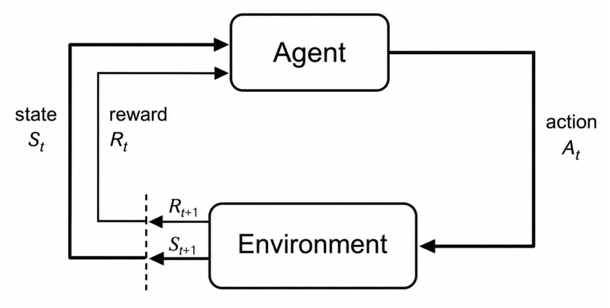
Figure 2.
Classification of Traffic Signal Control Methods
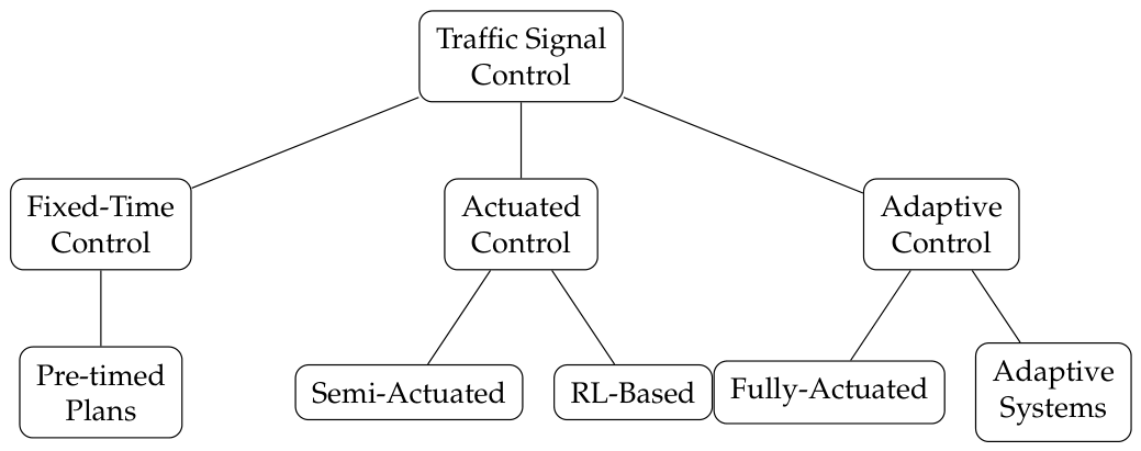
Figure 3.
The environment of our RL problem.
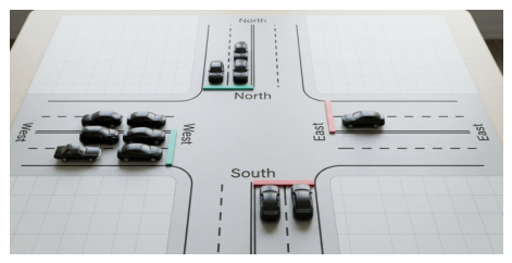
Figure 4.
Comparison of RL algorithms over 3000 training episodes.(a) Smoothed cumulative reward. (b) Average Queue Length. (c) Vehicle throughput. (d) Vehicle throughput. (e) Final Performance Comparison. (f) Normalised reward convergence .
Figure 4.
Comparison of RL algorithms over 3000 training episodes.(a) Smoothed cumulative reward. (b) Average Queue Length. (c) Vehicle throughput. (d) Vehicle throughput. (e) Final Performance Comparison. (f) Normalised reward convergence .
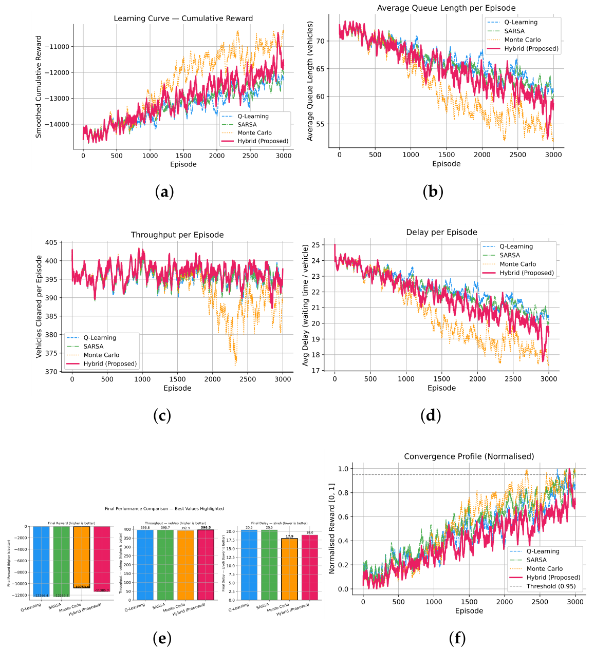
Figure 5.
Traffic control optimal:Multi-algorithm comparaison.
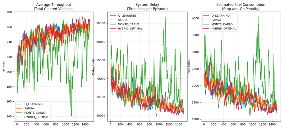
Figure 6.
Comparison of RL Algorithms across 10000 training episodes. (a) Evolution of the average delay. (b) Queue length. (c) Waiting time. (d) Throughput.
Figure 6.
Comparison of RL Algorithms across 10000 training episodes. (a) Evolution of the average delay. (b) Queue length. (c) Waiting time. (d) Throughput.
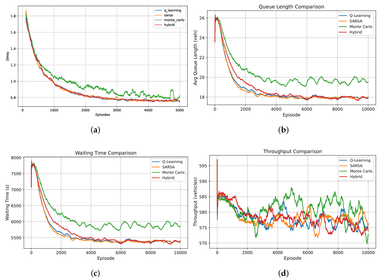

Table 1.
Performance comparison of the 4 RL algorithms.
| Method | Final Reward | Final Delay (s/veh) | Throughput (veh/ep) | Avg. Queue | Conv. Episode |
|---|---|---|---|---|---|
| Q-Learning | 2764 | ||||
| SARSA | 2718 | ||||
| Monte Carlo | 2875 | ||||
| Hybrid (ours) | 2938 |
Table 2.
Scientific benchmark report for the last 100 episodes.
| Algorithm | Avg. Reward | Std. Dev. Reward | Avg. Waiting Time (s) | Min. Waiting Time (s) | Max. Waiting Time (s) |
|---|---|---|---|---|---|
| Q-Learning | 245 | 407 | |||
| SARSA | 233 | 436 | |||
| Monte Carlo | 244 | 412 | |||
| Hybrid | 239 | 382 |
Disclaimer/Publisher’s Note: The statements, opinions and data contained in all publications are solely those of the individual author(s) and contributor(s) and not of MDPI and/or the editor(s). MDPI and/or the editor(s) disclaim responsibility for any injury to people or property resulting from any ideas, methods, instructions or products referred to in the content. |
© 2026 by the authors. Licensee MDPI, Basel, Switzerland. This article is an open access article distributed under the terms and conditions of the Creative Commons Attribution (CC BY) license (http://creativecommons.org/licenses/by/4.0/).
Copyright: This open access article is published under a Creative Commons CC BY 4.0 license, which permit the free download, distribution, and reuse, provided that the author and preprint are cited in any reuse.


