P versus NP: Computation as Counting over Finite Relational Substrate

1. Introduction

$\mathrm{P}$ versus $\mathrm{NP}$ asks whether every decision problem whose solutions can be verified in polynomial time can also be solved in polynomial time, that is, whether finding is as easy as checking. Built on the measure-based foundations of complexity [1] and prefigured in Gödel’s study of the length of proofs [2], the question was made precise by Cook and, independently, Levin: satisfiability is $\mathrm{NP}$-complete, so a single polynomial-time algorithm for it would collapse $\mathrm{NP}$ into $\mathrm{P}$ [3,4]. Karp’s reductions exhibited the reach of that collapse across combinatorial mathematics [5]. The question is open, and its very difficulty is now the subject of a mature theory.

1.1. Approaches and Barriers

Three bodies of work organise what is known. Structural theory fixes the classes intrinsically: by Fagin’s theorem $\mathrm{NP}$ is existential second-order logic, so a certificate is a witnessing structure and verification its evaluation [6]. Proof complexity recasts the dual side: by Cook and Reckhow, $\mathrm{NP}=\mathrm{coNP}$ if and only if some propositional proof system is polynomially bounded, turning the question into the existence of short proofs and, through bounded arithmetic, into the bounded provability of feasibility [7,8]. The matching problem of finding a short proof is automatizability, where the results are negative under cryptographic assumptions: strong Frege systems are not automatizable unless basic cryptography breaks, and even resolution is $\mathrm{NP}$-hard to automate [9,10,11].

Cryptography supplies both the candidate hardness and the average-case picture. Public-key cryptography rests on one-way functions, computable forward but not invertible, with the discrete logarithm and factoring the canonical instances [12]; their existence already gives $\mathrm{P}\ne \mathrm{NP}$, and Impagliazzo’s worlds chart the regimes between worst-case and average-case hardness [13]. The same instances fix the model-dependence of the question: factoring and the discrete logarithm, infeasible classically, are polynomial-time for a quantum observer through Shor’s algorithm [14], so any hardness claim is relative to a committed computational model.

Against this, three barriers constrain what a separation can be. Relativization shows the question flips under oracles, so a proof must use non-relativizing, machine-specific structure [15]. The natural-proofs barrier shows that a property both constructive and large would break pseudorandom generators, so a proof cannot rest on a generic feature of random functions [16]. Algebrization extends the oracle obstruction to algebraic oracles [17]. Taken together [18], the barriers point one way: a resolution must exploit the specific structure of computation, not a generic or oracle-level feature.

1.2. The Finite Substrate

The finite ring continuum (FRC) framework supplies such structure [19]. It is finitist: arithmetic is carried by a finite relational algebra, and the continuum is a degenerate idealisation of it, as “real” analysis is a degenerate case of discrete analysis [20]. Its foundations paper establishes one fact about a finite relational substrate [21]: as a totality the carrier $\Omega$ is complete and decidable, but an internal observer, a proper finite part with a bounded comprehension horizon, can neither represent the whole nor reach more than a vanishing fraction of its truths. Incompleteness is not abolished by finitude; it migrates from the truth of the totality to the reach of the observer. That gap is the horizon clause, and the Riemann, Goldbach, and $\mathrm{P}$-vs-$\mathrm{NP}$ residues are its three instances [21,22]. The horizon is a boundary of feasibility, not of truth: a statement is in or out of view by its resource cost, so “unprovable” reads as “not feasibly derivable within the horizon.” This places the question in bounded arithmetic and proof complexity, not in Gödel undecidability, which is vacuous over the finite substrate [7,8,21].

1.3. The Reading

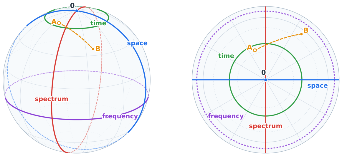
On this substrate computation is forward counting along a chosen representation, the hyperoperation ladder carried by the additive, spectral, and scale charts. A certificate is a near-representation: data exhibiting a chart in which a remote target sits within the horizon. $\mathrm{NP}$ asks only that such a near-representation exist; $\mathrm{P}$ asks that it be forward-constructible from within the horizon. The whole question is whether finding is as feasible as checking. Geometrically (Figure 1) the carrier is a shell with the observer at its pole, a near-representation a short geodesic to the target, $\mathrm{NP}$ that the geodesic exists and $\mathrm{P}$ that it is forward-findable.

1.4. Contribution

This paper works the third instance out. The reading reproduces standard complexity faithfully (Theorem 2) and connects, under exact substitutions, to proof complexity, automatizability, and one-way functions; its crisp form is a theorem, $\mathrm{P}=\mathrm{NP}$ exactly when every witness is as feasible to find as to check (Theorem 3, Lemma 1). The find-versus-exist gap is the uniformity of chart selection, not the existence of a localizing chart (Proposition 3), and the selector that would close it is a natural property barred under cryptographic hardness (Proposition 8). The directional core is native to the substrate: the hyperoperation ladder closes after four roles, the descent is the inverse of the last, the discrete logarithm, and the single time arrow of the drive is its irreversibility (§Section 6, §Section 7). The conclusion is stated in the programme’s terms: $\mathrm{P}$ versus $\mathrm{NP}$ is the computational face of the horizon clause, and its uniform certificate is $\Omega$-hard, decided by the totality yet below the bounded observer’s horizon. Section 2, Section 3 and Section 4 fix the language; §Section 5 states the crisp form and its automatizability face; §Section 6, Section 7 and Section 8 develop the one-way descent, the ladder closure, and the classical/quantum transform map; §Section 9 states the scope against the barriers; §Section 10 ties the result to the horizon clause. A geometric reading, the carrier as a shell and computation as geodesic navigation (Figure 1), runs throughout.

2. Computation as Counting Along a Representation

The ladder succession → addition → multiplication → exponentiation (each operation the iterate of the previous) is the Grzegorczyk/Ackermann hierarchy, built into the substrate. Addition steps the additive meridian; multiplication steps the scale (phase) cycle, which is addition in the discrete-logarithm chart; the scale operator $\widehat{H}=-\mathrm{i}(x{\partial }_x+\frac{1}{2})$ generates the dilation that climbs one level to the next [22]. The three representation domains the programme already uses — space (additive position), spectral (additive frequency, Fourier), scale (multiplicative, Mellin) — are distinct counting domains, and the Gauss and Mellin transforms are the paths between them. The ladder closes after these four roles: a fifth step, repeated exponentiation, is iteration of a finite power map and so returns to counting (Section 7), so the representation is built from four primitive operations, not an unbounded tower.

Read geometrically, these charts are faces of one finite carrier shell (Figure 1). The observer is the pole; the additive (space) and quarter-turn (spectrum) meridians and the time and frequency latitudes are four charts of the same surface, related by quarter-turns. A computation is navigation along a geodesic and its cost is geodesic length; the representation graph defined next is the discretisation of this surface, with $G_R$-distance the geodesic metric. We use the symmetry-complete carrier ${\mathbb{F}}_{13}$ only as a reference shape: the operative carrier is $\Omega \sim {10}^{122}$, and the sphere is the continuous shadow of the discrete graph, not a claim that one computes on a thirteen-point globe.

Definition 1 

(Representation, graph, cost). A representation is a triple $R=(E_R,O_R,c_R)$: an encoding $E_R$ of instances as strings over a finite alphabet, a finite set $O_R$ of elementary operations (partial maps on strings, each applied in one step), and the induced cost $c_R(x\to t)$, the least number of $O_R$-applications carrying $E_R\left(x\right)$ to a target t. The representation graph $G_R$ has strings as vertices and one edge per applicable operation; $c_R$ is graph distance. R is admissible if it and a standard machine simulate each other with polynomial overhead: each operation of $O_R$ runs in $\mathrm{poly}(\ell )$ standard steps, and each standard-machine step is an R-derivation of $\mathrm{poly}(\ell )$ operations. Cost is counted in bit operations, and $\mathrm{poly}$ is polynomial in the length of the input encoding: $\ell ={log}_{2}P$ for a carrier element, and n for an explicitly stored length-n object such as the vectors of §Section 8.

Claim 1 

(Representation-relativity of cost). Cost is a function of the (target, representation) pair, not of the target alone. A target far in one chart can be near in another; the transform between charts is itself a (possibly costly) path. Hence “within the horizon” is a predicate on pairs, and the search for a cheap representation is part of the problem, not prior to it.

Table 1. The operational vocabulary read as geometry on the shell of Figure 1.

operational term	object on the carrier shell
representation R	a chart on the shell
instance; identity 0	a point; the pole (the observer)
cost $c_R(x\to t)$	geodesic length
certificate / near-representation	a short geodesic (a chart where the target is near)
$\mathrm{NP}$	a short geodesic to the target exists
$\mathrm{P}$	that geodesic is forward-findable from the observer
verification; search	tracing a given geodesic; finding it without its far end
comprehension horizon H	the observer’s horizon (the equator)
totality / endpoint oracle	the whole shell, including shells past the horizon
ascent $a_P$; descent $d_P$	forward with the arrow; the inverse, against it
one-way function	a geodesic short to trace, not to find
single arrow of the drive	the orientation of the shell

Table 1. The operational vocabulary read as geometry on the shell of Figure 1.

operational term	object on the carrier shell
representation R	a chart on the shell
instance; identity 0	a point; the pole (the observer)
cost $c_R(x\to t)$	geodesic length
certificate / near-representation	a short geodesic (a chart where the target is near)
$\mathrm{NP}$	a short geodesic to the target exists
$\mathrm{P}$	that geodesic is forward-findable from the observer
verification; search	tracing a given geodesic; finding it without its far end
comprehension horizon H	the observer’s horizon (the equator)
totality / endpoint oracle	the whole shell, including shells past the horizon
ascent $a_P$; descent $d_P$	forward with the arrow; the inverse, against it
one-way function	a geodesic short to trace, not to find
single arrow of the drive	the orientation of the shell

2.1. The Two Quarter Turns and the Four Charts

The carrier supports two group structures, and the four charts are the two Fourier pairs they carry. On the additive group $({\mathbb{F}}_{\Omega },+)$ the position chart space and its dual spectrum are paired by the additive (Gauss) transform, with additive character $\psi \left(x\right)=e^{2\pi \mathrm{i}kx/\Omega }$. On the multiplicative group $({\mathbb{F}}_{\Omega }^{\times },·)\cong (C_{\Omega -1},+)$ the scale cycle time and its dual frequency are paired by the multiplicative (Mellin) transform, with multiplicative character ${\chi }_{\nu }\left(\theta \right)=e^{2\pi \mathrm{i}\nu \mathrm{ind}\left(\theta \right)/(\Omega -1)}$. Geometrically these are the shell’s two quarter-turns: the transverse turn between the through-pole meridians space and spectrum, and the longitudinal turn between the latitudes time and frequency, the meridional tilt that unfolds the near-pole time cycle into the equatorial frequency circle. Frequency stands to time as spectrum stands to space; the additive turn is the finite Fourier transform, and the longitudinal turn is the one developed here.

Proposition 1 

(The longitudinal quarter turn). The longitudinal turn is the multiplicative discrete Fourier transform on $C_{\Omega -1}$. It diagonalises the scale shift $\theta \mapsto g\theta$ (multiplication by a generator g): the multiplicative characters ${\chi }_{\nu }$ are its eigenvectors, with the $(\Omega -1)$-th roots of unity as the (distinct) eigenvalues, and the eigen-index ν is the frequency. In the continuum shadow it diagonalises the dilation generator $\widehat{H}=-\mathrm{i}(x{\partial }_x+\frac{1}{2})$, with eigenfunctions $x^{-1/2+\mathrm{i}\nu }$ of eigenvalue ν, so the frequency chart is the spectrum of $\widehat{H}$.

Proof. 

The scale shift is the cyclic shift on $C_{\Omega -1}$, a circulant, diagonalised by the character matrix; with $\zeta$ a primitive $(\Omega -1)$-th root of unity, ${\chi }_{\nu }\left(g^t\right)={\zeta }^{\nu t}$ gives $S{\chi }_{\nu }={\zeta }^{\nu }{\chi }_{\nu }$ with the ${\zeta }^{\nu }$ distinct (verified exactly over ${\mathbb{F}}_p$, longitudinal_turn.py). For the generator, $\widehat{H}{x}^{-1/2+\mathrm{i}\nu }=-\mathrm{i}\left[(-\frac{1}{2}+\mathrm{i}\nu )+\frac{1}{2}\right]x^{-1/2+\mathrm{i}\nu }=\nu x^{-1/2+\mathrm{i}\nu }$ (verified symbolically, ibid.).    □

Remark 1 

(The Gauss sum couples the two turns). The turns are not independent. The Gauss sum $g\left(\chi \right)={\sum }_{\theta }\chi \left(\theta \right)\psi \left(\theta \right)$ is the matrix element pairing an additive character (spectrum) with a multiplicative one (frequency), and for χ non-trivial ${\left|g\left(\chi \right)\right|}^2=\Omega$ (by the exact additive-character telescoping,longitudinal_turn.py). The full transform factors through both turns with the Gauss sum as their off-diagonal, and the modulus $\&\#x003A9;$ is the equatorial radius: the frequency latitude sits at the $\&\#x003A9;$ scale, the edge of the spectral window the programme works in [22].

3. The Comprehension Horizon

A statement is in view iff it has a derivation within the horizon in the current representation. By Claim 1 a change of representation can move the same statement inside or outside. This is the feasibility reading the companion isolates: the substrate decides everything as a totality, the bounded observer reaches only what fits under its horizon [21]. Geometrically (Figure 1, right) the horizon is the limb, near the equator, of the observer’s perspective view: the visible disc is what lies within reach, while the southern shells beyond it are decided by the totality but folded out of sight. Two bounds must be distinguished.

Definition 2 

(Per-instance and absolute horizons). The per-instance feasible horizon is a function $H(\ell )$ of the input length $\ell =|E_R\left(x\right)|$; the feasible regime is H polynomial. The absolute horizon ${\Omega }^{1/4}$ is the observer’s total step budget in the finite totality, capping $\ell \lesssim log\Omega$. They are nested: the absolute horizon bounds how much computation exists at all, the per-instance horizon is feasibility within it. The complexity classes below use the per-instance polynomial horizon; the totality, able to run ${\Omega }^{O\left(1\right)}=exp\left(O(\ell )\right)$ steps, is the endpoint-given oracle.

4. Proof as a Bounded Path; Certificate as a Near-Representation

A proof connecting axioms (near, in-horizon) to a theorem (far) by a chain of counting steps is the proof-complexity object; its length is the resource [7]. A certificate is a near-representation: data exhibiting a chart in which the far target sits under H, so that verification is the cheap traversal of a given bridge. This is the descriptive picture made standard by Fagin’s theorem [6]: $\mathrm{NP}$ is existential second-order logic, “there is a witnessing structure”, and the witnessing structure is precisely the near-representation. Existence of the witness is $\mathrm{NP}$; its feasibility-bounded discovery is the open matter. The framework re-describes standard complexity rather than replacing it.

Definition 3 

(The classes in a representation). L is forward-decidable in R within H if a $\mathrm{poly}(\ell )$-time uniform rule selects from each string its next operation and, for every x, the resulting deterministic forward path reaches the decision bit $[x\in L]$ within $H(\ell )$ steps of $E_R\left(x\right)$; write ${\mathrm{P}}_R$ for the languages forward-decidable within a polynomial horizon. L is certified-reachable (${\mathrm{NP}}_R$) if there is a polynomial p with $x\in L$ iff some certificate w, $\left|w\right|\le p(\ell )$, places “accept” within distance $\le H(\ell )$ of $(E_R\left(x\right),w)$ for a polynomial horizon. The distinction is the find-versus-exist axis: ${\mathrm{P}}_R$ asks the forward law to reach the answer, ${\mathrm{NP}}_R$ only that a short certified path exist.

Theorem 2 

(Faithfulness). For every admissible representation R, ${\mathrm{P}}_R=\mathrm{P}$ and ${\mathrm{NP}}_R=\mathrm{NP}$, the classes representation-invariant (Remark 2).

Proof.$(\subseteq )$ For ${\mathrm{P}}_R$, a deterministic R-derivation of length $\le H(\ell )$ whose operations are each simulable in $\mathrm{poly}(\ell )$ runs in $\mathrm{poly}(\ell )·H(\ell )=\mathrm{poly}(\ell )$ standard steps, so forward-decidability within a polynomial horizon gives $L\in \mathrm{P}$. For ${\mathrm{NP}}_R$, the verifier guesses the certificate together with the $\le H(\ell )$-step sequence of R-operations and checks each transition, every intermediate encoding $\mathrm{poly}(\ell )$-bounded, so the guess-and-verify is $\mathrm{poly}(\ell )$ and $L\in \mathrm{NP}$. $(\supseteq )$ Admissibility is two-way: each standard step is a $\mathrm{poly}(\ell )$-length R-derivation. A polynomial-time decision (resp. verification) on the standard machine is a computation of polynomial length, which this simulation rewrites as a deterministic R-derivation of polynomial length reaching the decision bit (resp., with the certificate, “accept”); so $\mathrm{P}\subseteq {\mathrm{P}}_R$ and $\mathrm{NP}\subseteq {\mathrm{NP}}_R$ for every admissible R, with the Church–Turing invariance of polynomial time [3].    □

Corollary 1 

(Robust class, relative cost). The classes ${\mathrm{P}}_R,{\mathrm{NP}}_R$ are representation-invariant; what varies with R (Claim 1) is the cost of a specific target and whether it is near within a fixed budget. A certificate is a representation in which the far target is near: supplied($\mathrm{NP}$) rather than forward-constructed($\mathrm{P}$).

Remark 2 

(Faithfulness is to the class structure; the asymptotic classes are its idealisation). Theorem 2 is read on the carrier family of Definition 7, not at one length: the carrier classes are $\mathrm{P}$ and $\mathrm{NP}$, carrying the relations that define them (closure under polynomial reductions, search-to-decision, the find-versus-check gap), and the textbook asymptotic classes are their degenerate idealisation, recovered by dropping finitude, in the sense that the continuum is a degenerate case of the discrete [20]. There is no larger class above them to truncate: the framework declines a tower of carriers ${\Omega }_s$ with $s\to \infty$, a completed sequence of stages reinstating the potential infinity the foundational programme forecloses [21]. Finitude is the setting, not a limit to be removed. A fixed length does admit, for each language, a decision table; but for inputs of length $\le \frac{1}{2}{log}_2\Omega$ that table has $\sim \&\#x003A9;$ entries, a sub-carrier object beyond the comprehension horizon ${\Omega }^{1/4}$, so “decidable by table” is exactly decided by the totality, unreachable below the horizon: the horizon clause again, not a route around it.

5. $\mathrm{P}$ Versus $\mathrm{NP}$: Finding Versus Checking

Both verification and search run forward in counting steps; the asymmetry is information about the endpoint. $\mathrm{NP}$ supplies the far target with a bridge and asks for traversal; $\mathrm{P}$ must build the bridge from the near side without being told the far endpoint. We make this exact, and identify its proof-complexity face. On the shell (Figure 1) the certificate is a short geodesic from the observer to the target: $\mathrm{NP}$ is that it exists, $\mathrm{P}$ that forward navigation finds it. A short geodesic is still a path, never a jump. The gap is its findability, not its existence.

Definition 4 

(Search problem; forward-constructibility). For $L\in \mathrm{NP}$ with verifier V and witness bound p, the search problem ${\mathrm{Search}}_V$ maps an instance x to some w with $\left|w\right|\le p\left(\right|x\left|\right)$ and $V(x,w)=1$ if one exists, and to ⊥ otherwise. The near-representation for L is forward-constructible iff ${\mathrm{Search}}_V\in \mathrm{FP}$.

Theorem 3 

(Crisp form). $\mathrm{P}=\mathrm{NP}$ if and only if ${\mathrm{Search}}_V\in \mathrm{FP}$ for every $L\in \mathrm{NP}$; equivalently, for $\mathrm{SAT}$.

Proof.$(\Leftarrow )$ If ${\mathrm{Search}}_V\in \mathrm{FP}$ then $L\in \mathrm{P}$: run the search and accept iff it returns a witness. $(\Rightarrow )$ Suppose $\mathrm{P}=\mathrm{NP}$. For $\mathrm{SAT}$ the decision problem is in $\mathrm{P}$, and a satisfying assignment is built by self-reduction: fix the variables in turn, at each step testing in $\mathrm{P}$ whether the partially-assigned formula remains satisfiable and keeping a value that preserves satisfiability. The result is a witness produced in polynomial time, so ${\mathrm{Search}}_{\mathrm{SAT}}\in \mathrm{FP}$; every $\mathrm{NP}$ search reduces to it by the witness-preserving Cook–Levin reduction.    □

Thus $\mathrm{P}=\mathrm{NP}$ exactly when a near-representation is as feasible to find as to check. Its proof-complexity face is automatizability.

Definition 5 

(Proof system; p-bounded; automatizable). A propositional proof system is a polynomial-time onto map $\Pi :{\{0,1\}}^{*}\to \mathrm{TAUT}$. It isp-boundedif every $\tau \in \mathrm{TAUT}$ has a Π-proof of size $\mathrm{poly}\left(\right|\tau \left|\right)$, and automatizable if some algorithm outputs a Π-proof of any $\tau \in \mathrm{TAUT}$ in time $\mathrm{poly}\left(\left|\tau \right|+s_{\Pi }\left(\tau \right)\right)$, where $s_{\Pi }\left(\tau \right)$ is the least size of a Π-proof of τ.

Lemma 1 

(Witness–automatization dictionary). For $L\in \mathrm{NP}$ with verifier V, let ${\Pi }_V$ be the certificate system for L (a witness system, not a propositional system for $\mathrm{TAUT}$) in which a proof of “x has a witness” is a w with $V(x,w)=1$. Then ${\mathrm{Search}}_V\in \mathrm{FP}$ iff ${\Pi }_V$ is automatizable. Hence, by Theorem 3, $\mathrm{P}=\mathrm{NP}$ iff every witness system is automatizable; the substantive find-versus-check gap appears on strong propositional systems for $\mathrm{TAUT}$(the $\mathrm{coNP}$ side), quantified in Remark 3.

Proof. 

A ${\Pi }_V$-proof of x is a witness w with $\left|w\right|\le p\left(\right|x\left|\right)$, so $s_{{\Pi }_V}\left(x\right)\le p\left(\right|x\left|\right)$; automatizing ${\Pi }_V$ means producing such a w in time $\mathrm{poly}\left(\right|x|+s_{{\Pi }_V}\left(x\right))=\mathrm{poly}(\left|x\right|)$, which is ${\mathrm{Search}}_V\in \mathrm{FP}$, and conversely.    □

Proposition 2 

(Finding collapses to checking). If $\mathrm{P}=\mathrm{NP}$ then every propositional proof system is automatizable.

Proof. 

For fixed $\tau$ and budget s, the predicate “$\tau$ has a $\Pi$-proof of size $\le s$” is in $\mathrm{NP}$ (guess the proof, verify $\Pi$ in polynomial time), hence in $\mathrm{P}$. Construct the proof bit by bit by self-reduction, querying at each step whether the current prefix extends to a valid proof of size $\le s$; raising s to the least proof size $s_{\Pi }\left(\tau \right)$ yields a proof in time $\mathrm{poly}\left(\right|\tau |+s_{\Pi }\left(\tau \right))$.    □

Remark 3 

(The gap is finding-versus-existing, and it rests on the descent). The converse of Proposition 2 fails: the truth-table system is automatizable yet not p-bounded. Hence the existence of a short proof (p-boundedness, equivalent to $\mathrm{NP}=\mathrm{coNP}$ by Cook–Reckhow [7]) and its discovery (automatizability) are distinct, and their difference is exactly the find-versus-check asymmetry of Theorem 3. The known separations make this concrete and tie it to §Section 6: Extended Frege is not automatizable unless $\mathrm{RSA}$ is insecure [9], bounded-depth Frege is not automatizable unless factoring and Diffie–Hellman are feasible [10], and resolution is $\mathrm{NP}$-hard to automate [11]. Each conditions the find-versus-check gap on the hardness of the substrate’s descent: factoring and the discrete logarithm. The automatizability axis and the one-way axis (§Section 6) are one phenomenon in two literatures.

The search-to-decision reduction for $\mathrm{NP}$-complete problems is Theorem 3 read from the other side; the automatizability lower bounds are the same find-versus-check gap, conditioned on the one-way descent the substrate supplies natively.

On the shell every chart coordinatises the whole carrier, so every target is near the origin in some chart; the content of $\mathrm{P}$ vs $\mathrm{NP}$ is not the existence of a localizing chart but whether one is named by a uniform forward law.

Definition 6 

(Localizing chart; selector). For $L\in \mathrm{NP}$ with verifier V, an admissible chart R(Definition 1)localizes$x\in L$ if some witness w, $V(x,w)=1$, lies within the polynomial horizon in R: $c_R(\mathbf{0}\to w)\le \mathrm{poly}(\ell )$. A constructive localising selector is a map $x\mapsto \langle R_x\rangle$ in $\mathrm{FP}$ emitting an admissible chart together with a canonical $\mathrm{poly}(\ell )$-time forward rule whose orbit from $\mathbf{0}$ reaches such a witness in $\mathrm{poly}(\ell )$ steps; equivalently it may output the witness itself or a $\mathrm{poly}(\ell )$-length path to it. Proximity alone is insufficient: a polynomial-radius ball may hold exponentially many points, so the selector must reach the witness, not merely place it near.

Proposition 3 

(Existence is free; the selector is the content). For every $L\in \mathrm{NP}$ and every $x\in L$ a localizing chart exists unconditionally. A constructive localising selector for every $L\in \mathrm{NP}$, equivalently for $\mathrm{SAT}$, exists if and only if $\mathrm{P}=\mathrm{NP}$; a selector for a single easy L does not suffice.

Proof. 

Existence. Fix any witness $w_x$ of x and let $R_x$ recentre the scale chart so that $w_x$ is one counting step from $\mathbf{0}$; then $c_{R_x}(\mathbf{0}\to w_x)=1$. The chart is admissible (a translation in the index ring), and $w_x$ enters only to name it, so the statement is unconditional and non-uniform. $(\Leftarrow )$ If $\mathrm{P}=\mathrm{NP}$ then ${\mathrm{Search}}_V\in \mathrm{FP}$ for every $L\in \mathrm{NP}$ (Theorem 3); the selector that runs the search and emits the recentring chart of the returned witness, with the one-step forward rule reaching it, is constructive and localizing. $(\Rightarrow )$ A constructive selector for $\mathrm{SAT}$ gives, on each x, $\langle R_x\rangle$ in $\mathrm{poly}(\ell )$ together with the forward rule whose $\le \mathrm{poly}(\ell )$ orbit reaches a witness; running it solves ${\mathrm{Search}}_{\mathrm{SAT}}\in \mathrm{FP}$, so $\mathrm{P}=\mathrm{NP}$ by Theorem 3. The quantifier is essential: a selector for an easy L alone leaves $\mathrm{Search}$ for harder languages untouched.    □

Remark 4 

(The lucky-chart objection). The objection “every target is near in some chart, so finding equals checking” fails on the quantifier Proposition 3 isolates: the localizing chart exists for free but is named by the answer, and entering it is itself a path, never a jump. No chart change is free (Claim 1). A witness’s coordinate ($O(\ell )$ bits) is not the cost of finding it. Three quantities differ: the naive orbit length (recovering m by stepping the cycle, up to $2^{\ell }$), the cost of a specified algorithm (baby-step–giant-step recovers m in $\sqrt{P}$, Section 6), and the minimum complexity of the descent (the open lower bound). The bijection $m\mapsto g^m$ onto the orbit ordinals is whatchart_localization.pyverifies; it is not a lower bound on any of the three. Short to name is not short to find; $\mathrm{P}$ vs $\mathrm{NP}$ asks whether the naming law is itself forward.

6. The Directional Asymmetry Is a One-Way Function

The hyperoperation ladder is easy to ascend and hard to descend. We make this exact on the carrier. On the shell the ascent runs with the arrow along the scale cycle (time); the descent is the geodesic against it. The single arrow is the orientation of the surface, and the one-way function is the upward path it denies to forward navigation.

Definition 7 

(Charts; ascent and descent; the carrier family). On the carrier ${\mathbb{F}}_P$ (P prime, bit-length $\ell =\lceil {log}_{2}P\rceil$) the additive chart $({\mathbb{F}}_P,+)$ and the scale chart $({\mathbb{F}}_P^{\times },·)\cong (C_{P-1},+)$ are related by discrete logarithm. With a fixed generator g, the ascent is modular exponentiation $a_P\left(j\right)=g^{j}modP$ (additive index → scale element); the descent is its inverse $d_P={\mathrm{dlog}}_g$. The carrier family is $\{{\mathbb{F}}_P:\ell ={log}_{2}P\le \frac{1}{2}{log}_2\Omega \}$; input size is ℓ, feasibility is $\mathrm{poly}(\ell )$, and the totality (running $2^{O(\ell )}\le {\Omega }^{O\left(1\right)}$ steps) is the endpoint-given oracle of Definition 2.

Theorem 4 

(Ascent is feasible). $a_P\left(j\right)=g^{j}modP$ is computable in $O(\ell )$ modular multiplications, hence in $\mathrm{poly}(\ell )$ bit operations.

Proof. 

Square-and-multiply: scan the $O(\ell )$ bits of j, alternating squarings and multiplications, each a $\mathrm{poly}(\ell )$-bit modular operation.    □

The descent has no such bound. Empirically (the accompanying dlog_asymmetry.py) the ascent time scales as $P^{+0.04}$ (flat in P, polynomial in ℓ) while the descent by baby-step–giant-step scales as $P^{+0.48}\approx \sqrt{P}=2^{\ell /2}$, exponential in ℓ; the descent/ascent ratio grows $58\to 3317$ over $P\sim {10}^5--{10}^9$. The asymmetry is exhibited, not assumed.

These costs place the descent on three separated scales. The feasibility budget is $\mathrm{poly}(\ell )$, which the descent exceeds. The per-instance descent by baby-step–giant-step is $\sqrt{P}=2^{\ell /2}$; for the carrier family ($P\le {\Omega }^{1/2}$, Definition 7) this is at most ${\Omega }^{1/4}$, the absolute horizon of Definition 2: superpolynomial in ℓ yet far below carrier scale, so no single descent is itself a carrier-scale object. Beyond both lies the uniform statement that no $\mathrm{poly}(\ell )$ inverse exists across the family, a lower bound with no per-instance witness. Residue 6 places the descent beyond the polynomial horizon; the uniform certificate is the below-horizon $\Omega$-hard residue (Section 10), carrier-scale by the bounded observer’s reach, not by the descent’s cost.

Definition 8 

(One-way family). A family $\left\{f_{\ell }\right\}$ is one-way if each $f_{\ell }$ is computable in $\mathrm{poly}(\ell )$ while, for every $\mathrm{poly}(\ell )$-time A, the carrier inputs x on which $A\left(f_{\ell }\left(x\right)\right)\in f_{\ell }^{-1}\left(f_{\ell }\left(x\right)\right)$ number at most a sub-horizon fraction of the carrier. This is the finite-totality reading of cryptographic one-wayness: the success count stays below the comprehension horizon, replacing the asymptotic notion of negligibility.

Theorem 5 

(One-way ⇒ separation). If a one-way family exists, then $\mathrm{P}\ne \mathrm{NP}$.

Proof. 

Inverting a $\mathrm{poly}$-computable f is the search problem for the verifier $V(y,x)=\left[f\right(x)=y]$, which runs in $\mathrm{poly}(\ell )$; so by Theorem 3, $\mathrm{P}=\mathrm{NP}$ would put this search in $\mathrm{FP}$, giving a $\mathrm{poly}(\ell )$-time inverter and contradicting one-wayness. Hence $\mathrm{P}\ne \mathrm{NP}$.    □

The substrate supplies the canonical candidate, not by analogy: its scale structure is built on the discrete logarithm, and the Gauss sums on which the programme’s spectral identities rest are defined through it [12,14,22].

Residue 6 

(The scale-descent residue: the computational horizon clause’s certificate). The scale-descent residue is the statement that the ascent family $\left\{a_P\right\}$, $a_P\left(j\right)=g^j$, on the carrier family of Definition 7 is one-way: it is $\mathrm{poly}(\ell )$(Theorem 4) and no $\mathrm{poly}(\ell )$ forward computation inverts it, the discrete logarithm $d_P$ being infeasible. Its status is Ω-hard (Section 10): decided by the totality, beyond the bounded observer. It is not a foundational assumption of the programme but the certificate of the computational horizon clause, derived to be Ω-hard from the ground and its forced pillars; the complexity literature, lacking the totality, posits the same statement as the discrete-logarithm hardness assumption, the bridge to which the conditional $\mathrm{P}\ne \mathrm{NP}$ below attaches (Theorem 5).

Corollary 2. 

If the scale descent is one-way (Residue 6), then $\mathrm{P}\ne \mathrm{NP}$ (Theorem 5).

Claim 7 

(FRC-native locus). The comprehension-horizon-plus-representation picture forces a one-way structure: ascent is a horizon-bounded forward count, descent its inverse below the horizon. $\mathrm{P}\ne \mathrm{NP}$ follows from Residue 6 (Theorem 5): the scale descent admits no $\mathrm{poly}(\ell )$ forward inverse. The implication is one-way; $\mathrm{P}\ne \mathrm{NP}$ is not known to require a one-way function. The single arrow of the drive is the structural reason for the residue, and the locus of any resolution: ascent runs with the arrow, while the descent is the time-reversed, Frobenius-conjugate branch a composed observer cannot freely take.

Remark 5 

(The descent is the inverse coordinate map of the scale chart). The ascent $a_P:j\mapsto g^j$ is the coordinate map of the scale chart, the bijection $C_{P-1}\to {\mathbb{F}}_P^{\times }$ carrying the time index to its multiplicative position; the descent $d_P=\mathrm{dlog}$ is its inverse, the reading of the index, a finite-cyclic-group coordinate and not the inverse of the multiplicative Fourier transform (which diagonalises the shift, Proposition 1). The single arrow orients the coordinate: advancing the index (multiplying by g) is forward-free, recovering it runs against the arrow. The frequency chart is where the descent forward-resolves, for the observer who can take the longitudinal turn forward and for no other (Proposition 7).

Remark 6 

(The scaling flow returns the doubled walk: an external theorem on the shell). The shell picture has an exact external counterpart. Eckmann and Tlusty [23] study a walk $W=R_N\dots R_1$ in $\mathrm{SO}\left(3\right)$ (equivalently $\mathrm{SU}\left(2\right)$) under the uniform angle scaling ${\omega }_j\mapsto \lambda {\omega }_j$, precisely the dilation flow generated by $\widehat{H}$ (Proposition 1), motion along the scale axis. Two facts result. First (their Lemma): the single scaled walk $W\left(\lambda \right)$ reaches the identity only on a measure-zero set of walks, because the identity is a single point of codimension 3 and a one-parameter family $\lambda \mapsto W\left(\lambda \right)$ generically misses it. This is the single-arrow obstruction (Claim 7) as a theorem: one forward parameter cannot reach a designated point. Second (their Theorem): the doubled walk satisfies ${\left[W\left(\lambda \right)\right]}^2=1$ for some $\lambda >0$, because it need only meet the codimension-1 manifold of ${180}^{\circ }$ rotations (the square-roots of the identity), which a one-parameter curve generically crosses; the returning λ is delivered by Minkowski’s convex-body theorem, non-constructively, and is exponentially large, $\lambda =2\pi n_0$ with $|n_0{|\lesssim (\ell /\epsilon )}^N$.

Read on the carrier this is the find–exist split of Proposition 3 exactly: a returning scaling exists unconditionally, but the witness is exponential and is produced by a pigeonhole/lattice existence argument, not a forward construction. The asymmetry is geometric. A designated target (a witness, a specified point) is codimension 3 and generically unreachable by the single scaling; the relaxed target, any involution, is codimension 1 and is met. Doubling reaches the manifold of half-returns; it does not reach a chosen point. The external theorem is thus on-shell evidence consonant with Residue 6: the scale descent is not forward-findable by a single dilation, and the one resource that returns the doubled walk is provably blind to the designated target a computation must hit. This is a geometric parallel and motivational evidence for the single-arrow obstruction, not itself a computational lower bound.

7. The Arithmetic-Hierarchy Closure: The Descent Inverts the Last Role

The ladder of Section 2 closes at four. Over ${\mathbb{F}}_{\Omega }$ every value is an $\Omega$-cardinality residue and every exponent an $(\Omega -1)$-cardinality residue, so the hyperoperation hierarchy that is unbounded over $\mathbb{N}$ has nowhere to grow: succession, addition, multiplication, and fixed-base exponentiation generate the carrier’s two cyclic structures and the bridge between them, and the fifth level folds back. Fixed-base exponentiation is the top role; its inverse, the discrete logarithm, is the single one-way step of Section 6.

Definition 9 

(The four primitive roles). On the carrier ${\mathbb{F}}_P$ with a fixed primitive generator g, the four generative levels of arithmetic are succession $\sigma \left(x\right)=x+1$, addition $T_a\left(x\right)=x+a={\sigma }^a\left(x\right)$, multiplication $S_m\left(x\right)=mx$ (m-fold addition), and fixed-base exponentiation $a_P\left(j\right)=g^j=S_g^j\left(1\right)$ (j-fold multiplication by g), the isomorphism of the index cycle $C_{P-1}$ onto ${\mathbb{F}}_P^{\times }$. Each level is the previous iterated with a fixed operand; counting is iterated succession, succession generates the additive law, and exponentiation bridges the additive and multiplicative cycles. The fourth level is the top, and its inverse is the discrete logarithm.

Proposition 4 

(Ladder closure). On the finite carrier the four levels of Definition 9 close the arithmetic hierarchy. They generate the carrier’s two cyclic structures, the additive $C_{\Omega }$ and the multiplicative $C_{P-1}$, with the exponential bridge $a_P$ between them. The fifth level, iterated exponentiation (tetration $j\mapsto g^{\left(g^{·}\right)}$), introduces no new primitive: every tower exponent is an element of ${\mathbb{F}}_P^{\times }$, read as an index in $C_{P-1}$, so tetration is exponentiation of a reduced index, and the power endomorphisms $P_k\left(g^m\right)=g^{km}$ are multiplication on that same index (Theorem 8). No third cyclic structure exists to host a fifth operation; the hierarchy unbounded over $\mathbb{N}$ closes at four over ${\mathbb{F}}_{\Omega }$, by finitude.

Proof. 

The field ${\mathbb{F}}_P$ carries its additive group $C_{\Omega }$ and its multiplicative group $C_{P-1}$; succession generates the first and a generator g the second, and $a_P:j\mapsto g^j$ is the canonical index map between them. Iterating $a_P$ composes this map with index reduction in $C_{P-1}$, a structure already present, and the endomorphism $P_k$ acts there as multiplication by k (Theorem 8); both stay within the two cyclic structures. Hence every operation reached by iteration is a composition of the four levels, and no fifth primitive arises. The closure is structural, a statement about which operations the carrier supports, not about their cost: the infeasibility of inverting the fourth level is the separate matter of Residue 6.    □

So a representation (Definition 1) is assembled from the four levels of Definition 9, the fourth being fixed-base exponentiation whose ascent Section 6 uses, and whose inverse, the discrete logarithm, is the one-way step.

Theorem 8 

(Phase-index dynamics of the ascent). In the scale chart $x=g^m$(g a generator, $m\in C_{P-1}$)the power map acts on the index by $P_k\left(g^m\right)=g^{km}$, and its iteration by

$$P_k^r\left(g^m\right)=g^{k^{r}m},k^r\mathrm{read}\mathrm{in}{C}_{P-1}.$$

The ascent $a_P\left(j\right)=g^j$ is the orbit traversal $j\mapsto j+1$, i.e., $g^{j+1}=g·g^j$: one multiplication per counted step.

Proof. 

$P_k\left(g^m\right)={\left(g^m\right)}^k=g^{km}$. Assuming $P_k^r\left(g^m\right)=g^{k^{r}m}$, one further application gives $g^{k^{r+1}m}$, the exponent taken modulo the order $P-1$ of g. Verified over four carriers in closure_pnp.py.    □

The asymmetry of Section 6 now has a one-line cause: the ascent reads a count off a finite orbit; the descent must recover it.

Proposition 5 

(The one-way function is the inverse of the last role). Each forward level costs $O(\ell )$ modular operations: succession and addition are translations, multiplication is one modular product, and exponentiation $a_P\left(j\right)=g^j$ is $O(\ell )$ by square-and-multiply (Theorem 4). The discrete logarithm $d_P={\mathrm{dlog}}_g$ recovers the index m from $g^m$: the position of a point in the counted orbit of the fourth role. Hence the one-way family of Residue 6 is exactly the inverse of the single last primitive role, and all irreversibility in the closed ladder is localised to that one step. Empirically the descent/ascent operation ratio grows as $\sqrt{P}/\ell$(closure_pnp.py: $8\to 351$ over $P\sim {10}^4--{10}^8$).

This dissolves the circularity flagged in Remark 9. The model admits the four forward primitive roles and their polynomial compositions; the descent is not among them: it is the inverse of the fourth, the orbit-position problem the closure’s return to counting does not supply. Excluding a feasible descent is therefore not the stipulation of an operation forbidden by fiat; it is the statement that inverting the last primitive role is infeasible, which is precisely $\mathrm{dlog}\notin \mathrm{P}$. The single arrow of Claim 7 thereby acquires an arithmetic reading: the forward roles count up a closed ladder, and only the recovery of the count, against the orbit of the power map, runs against the arrow.

Remark 7 

(Compatibility with the transform map and the compression dichotomy). The index cycle is $C_{P-1}$, and the iterated power map’s orbit is the abelian hidden-subgroup datum on which Shor’s quantum Fourier transform acts [14], the same chart Proposition 7 marks as the hard classical case. The closure thus locates the descent exactly where Section 8 places it: forward-near in the frequency chart (the multiplicative Fourier of $C_{P-1}$, Proposition 1; a bounded-error quantum polynomial-time ($\mathrm{BQP}$) observer), arrow-bound in the classical time/scale chart. The power map is moreover a bijection of ${\mathbb{F}}_P^{\times }$ iff $gcd(k,P-1)=1$, and otherwise compresses its image to size $(P-1)/gcd(k,P-1)$(closure_pnp.py); in the bijective case it is efficiently invertible by $k^{-1}mod(P-1)$, so the one-way map is not the power map but the exponential $a_P:j\mapsto g^j$, whose inverse is the discrete logarithm (Remark 5).

8. The Transform Map: Which Charts Are Forward-Computable

Claim 1 makes “near” representation-relative; the operative question is which charts an observer reaches forward. On the structured (abelian) problems the answer is exact, and it is the classical/quantum line. In the shell’s terms the charts are the four domains, and Shor’s transform is the longitudinal quarter-turn from the time (scale) chart into the frequency chart (Proposition 1), where the descent geodesic shortens for a $\mathrm{BQP}$ observer; the classical/quantum line is the boundary between the shell’s two quarter-turns (Proposition 6).

Proposition 6 

(The two quarter turns as a structured classical–quantum correspondence). The transverse turn (space↔spectrum, the additive Fourier transform) is forward-computable classically on an explicit length-n vector (the fast Fourier transform and its inverse in $O(nlogn)$, Theorem 9), so problems diagonal in the spectrum chart lie in $\mathrm{P}$. The longitudinal turn (time↔frequency, the multiplicative Fourier transform on $C_{\Omega -1}$, Proposition 1) is the order/period transform. A $\mathrm{BQP}$ observer reaches its period through Shor’s order-finding, the quantum Fourier transform on an exponent register with measurement and classical post-processing [14], not by reading off a stored transform vector; under Residue 6 the arrow-bound classical observer cannot reach it (Proposition 7). The classical and quantum transforms have different input/output models: both are classically computable on an explicitly stored vector, and the quantum advantage is succinct state preparation and sampling, not a faster transform. This is therefore a structural correspondence between the two charts and the observers that reach them forward, not an identity of complexity-theoretic transforms: the transverse turn classical computation takes freely, the longitudinal turn it does not.

Definition 10 

(Forward-computable transform; transform-diagonalisable problem). A chart change T is forward-computable if both T and $T^{-1}$ lie in $\mathrm{P}$. A problem is transform-diagonalisable by T if in the T-chart its instances become a pointwise (diagonal) computation. This is well-defined for abelian/convolution and hidden-subgroup problems; it is not a feature of $\mathrm{NP}$ at large.

Theorem 9 

(Fourier-diagonalisable ⇒$\mathrm{P}$). A problem transform-diagonalisable by the finite additive Fourier transform is in $\mathrm{P}$: the FFT and its inverse are computable in $O(nlogn)$, so the target is forward-near in the spectrum chart.

Proof. 

Diagonalisation makes the T-chart computation pointwise, hence $O\left(n\right)$; with $T,T^{-1}$ the FFT pair in $O(nlogn)$ (forward-computable), the whole computation is $O(nlogn)$.    □

Empirically (the accompanying transform_charts.py): cyclic convolution costs $\Theta \left(n^2\right)$ in the position chart but $O(nlogn)$ through the spectrum chart (the same target far in one chart and near in the other, Claim 1 exhibited), and the transform itself is forward-computable and exact ($|T^{-1}Tx-x|\sim {10}^{-15}$ at $n=2^{16}$).

Lemma 2 

(Structured witness sets are forward-localizable). Suppose $L\in \mathrm{NP}$ has, for each x, a witness set presented as the solutions of an affine ${\mathbb{F}}_2$-system readable from x in $\mathrm{poly}(\ell )$. Then the constructive localising selector of Proposition 3 is explicit: Gaussian elimination returns a particular solution $w_0$ and a basis of the solution space, and the chart $w\mapsto w-w_0$ in that basis localizes the witnesses: the origin is a witness and every solution lies within $\le \mathrm{poly}(\ell )$ basis steps.

Proof. 

Gaussian elimination on the affine system is $\mathrm{poly}(\ell )$ and yields $w_0$ together with a solution-space basis of dimension $\le \mathrm{poly}(\ell )$; the emitted recentring chart is admissible and forward, places $w_0$ at $\mathbf{0}$, and puts every solution within that many counting steps, so the selector localizes x and produces a witness in $\mathrm{poly}(\ell )$.    □

The chart programme is constructive on the structured stratum: it reproduces the feasible islands (affine witness sets by Gaussian elimination, convolution-diagonal ones by the Fourier pair of Theorem 9) as explicit constructive selectors. The hidden-period extension of the same stratum is the longitudinal quarter-turn below, forward for a $\mathrm{BQP}$ observer and arrow-bound for the classical one; beyond these structured sets no constructive selector is known, the wall Section 9 ties to the natural-proofs barrier.

Proposition 7 

(The scale chart is the hard case). The discrete logarithm is the carrier’s native order/period instance: its diagonalising transform is the multiplicative (longitudinal) Fourier of Proposition 1, reached by a $\mathrm{BQP}$ observer through Shor’s order-finding [14] and, under Residue 6, not by the arrow-bound classical observer. Factoring is a related but distinct order-finding instance, modulo a composite rather than over the cyclic $C_{\Omega -1}$, and its classical hardness is not covered by Residue 6. On these structured instances the frequency chart is the one no classical forward computation reaches, while the additive (transverse) spectrum chart it does take. This is a correspondence on selected structured algorithms, not a complete classical/quantum boundary theorem.

The map covers the structured class treated here: Fourier-diagonalisable problems are forward-near (Theorem 9), the order/period problems require the scale chart (Proposition 7), and the boundary between them traces the classical/quantum line on these instances. It does not extend to a transform characterisation of all of $\mathrm{NP}$; none is known, and none is claimed.

9. What the Reading Delivers, and What It Relocates

The reading connects, under exact substitutions, to three pillars: proof complexity (§Section 4), automatizability (§Section 5), and one-way functions (§Section 6). It grounds the directional intuition in the substrate’s own scale/discrete-log map and time arrow. It is suggestive of $\mathrm{P}\ne \mathrm{NP}$ because the ascent/descent asymmetry is built into the hierarchy. The difficulty of $\mathrm{P}$ vs $\mathrm{NP}$ is its $\Omega$-hardness (§Section 10). One-way functions, if they exist, are sufficient for $\mathrm{P}\ne \mathrm{NP}$ (Theorem 5), and the carrier’s candidate is the infeasibility of the descent (Residue 6); the converse, that $\mathrm{P}\ne \mathrm{NP}$ requires one, is not known. The descent lies beyond the polynomial horizon (Theorem 5); its uniform certificate is the below-horizon $\Omega$-hard residue (Section 10), decided by the totality and beyond the bounded observer, the irreducible residue (Section 11). Two boundaries must be stated exactly.

9.0.0.1. Average-case versus worst-case.

One-way functions and the discrete-log/factoring instances are the average-case, $\mathrm{NP}\cap \mathrm{coNP}$ heart; $\mathrm{P}$ vs $\mathrm{NP}$ proper is the worst-case $\mathrm{NP}$-complete question [3], broader than the directional picture alone. The reading captures the cryptographic core (sufficient for $\mathrm{P}\ne \mathrm{NP}$), not the full worst-case statement.

9.0.0.2. Model-relativity.

Representation-relativity (Claim 1) is genuine but model-relative: a target far in one model can be near in another. Factoring is infeasible classically yet feasible in the frequency representation reached by the quantum Fourier transform [14]; the descent that is one-way for a classical observer is not one-way for a $\mathrm{BQP}$ observer. This is why $\mathrm{P}$ vs $\mathrm{NP}$ is posed for a fixed (classical) model, and why the horizon must be tied to a committed computational substrate.

9.0.0.3. Relation to the known barriers.

The reading is a reformulation and a locus, not a relativizing, natural, or algebrizing proof attempt, so the three meta-barriers do not apply to it as obstructions; it points where they say a resolution must point. Relativization [15] demands a non-relativizing, structure-specific argument; the discrete-log descent on the committed carrier is exactly such specific structure. The natural-proofs barrier [16] forbids large, constructive distinguishers; the reading’s content is the non-genericity of the descent (its alignment with the single arrow), not a natural property of random functions (Proposition 8). Algebrization [17] closes the algebraic-oracle extension of relativization; the carrier’s scale arithmetic is the concrete algebraic object, not an oracle. The reading thus directs attention to the specific finite structure the barriers single out as necessary, without itself being a technique the barriers exclude. In one image: relativization treats the shell as a featureless sphere, an oracle with no arrow; natural proofs forbid a large generic marking, whereas the hardness is the non-generic alignment with the arrow; algebrization adds an algebraic oracle the carrier’s own scale arithmetic replaces. A resolution must therefore read the oriented scale geometry the figure foregrounds.

Proposition 8 

(A universal selector would break the one-way family). Suppose a single constructive localising selector(Definition 6)localizes the witness sets of every $\mathrm{P}$-samplable instance family. Applied to the inversion family $V(y,w)=\left[f\right(w)=y]$ of a one-way f it inverts f in $\mathrm{poly}(\ell )$; so under Residue 6 no such universal selector exists, and by Proposition 3 its non-existence is equivalent to $\mathrm{P}\ne \mathrm{NP}$. By analogy with Razborov–Rudich [16] the selector is a constructive test that succeeds across the family, so a separation must rest on a non-natural obstruction aligned with the single arrow rather than a generic marking; the density (largeness) their theorem requires is not established here, so the natural-proofs reading is an analogy, not an instance.

Proof. 

A universal constructive selector outputs a witness for every x in $\mathrm{poly}(\ell )$; on the inversion family of a one-way f it inverts f, contradicting one-wayness (Theorem 5). The equivalence to $\mathrm{P}\ne \mathrm{NP}$ is Proposition 3. The test runs in $\mathrm{poly}(\ell )$ (constructive) and succeeds across the chosen family; that success over a samplable family is not the truth-table density Razborov–Rudich require, so the surviving obstruction is read, by analogy, as the non-generic arrow-alignment of Claim 7.    □

10. The Horizon Clause

The reading is the feasibility instance of the companion’s horizon clause [21]: a statement decided by the totality but certifiable by the bounded observer only below the horizon. We name such a statement Ω-hard: the totality decides it (here in ${\Omega }^{O\left(1\right)}$ steps) and an instance witness is checkable at sub-carrier scale, but its uniform, forward-findable certificate is carrier-scale, below the bounded observer’s horizon. An $\Omega$-hard statement is decidable, not undecidable; it is settled only at the scale of the whole, and is the carrier-scale analogue, relative to the bounded part, of $\mathrm{NP}$-hardness. The Carrier is the totality, and every residue on it lies either above the comprehension horizon, where the bounded observer can express and prove it, or below, where it cannot. The uniform certificate of the descent lies below: held exactly by the totality, beyond the observer’s reach by the projective incompleteness of every bounded reading. Here $\Phi$ is “the scale descent is forward-invertible”: the totality contains the inverse (it can factor, it can take discrete logarithms, in ${\Omega }^{O\left(1\right)}$ steps), while the H-bounded observer cannot reach it; $\mathrm{P}=\mathrm{NP}$ would make this $\Omega$-hard residue feasibly findable, not merely checkable. The Riemann residue (completeness of the on-line spectrum) and the Goldbach residue (the uniform per-n bound) are the same clause in the spectral and additive domains [22]; $\mathrm{P}$ vs $\mathrm{NP}$ is its computational face. In every case the obstruction is neither falsity nor undecidability of truth but the gap between a complete totality and a bounded part: the horizon, the programme’s one recurring residue, $\Omega$-hard in each domain. Ontologically this is the finite-because-complete substrate of the foundational programme [21]: the carrier has no outside, so infinity enters only as the observer’s epistemic horizon, never as an ingredient. The surface of Figure 1 is the complete whole, and each horizon clause (spectral, additive, computational) is a place where the bounded part meets its edge on it.

Remark 8 

(Frequency is the Hilbert–Pólya spectrum). The frequency chart, the spectrum of the dilation generator $\widehat{H}$ (Proposition 1), is where the non-trivial zeros sit as frequencies, the Hilbert–Pólya/Berry–Keating reading of the Riemann residue [22,24,25]. The longitudinal turn is the same Fourier the explicit formula performs, carrying the primes of the space chart to the zeros of the frequency chart. The Riemann residue’s spectrum and the $\mathrm{P}$-vs-$\mathrm{NP}$ frequency chart are thus one domain, and the horizon clause’s spectral and computational faces meet on the single $\widehat{H}$-axis.

11. Status: What Is Settled, and the Irreducible Residue

The operational core is settled below the horizon. The model is faithful to standard complexity (Theorem 2); the core is the theorem (Theorem 3) with its automatization dictionary (Lemma 1, Proposition 2); the forward-computable charts are mapped on the structured class (Theorem 9, Lemma 2, Proposition 7); the find–exist gap is the uniformity of chart selection, not the existence of a chart (Proposition 3), and the selector that would close it is a natural property barred under cryptographic hardness (Proposition 8). The arithmetic-hierarchy closure (Section 7) is the last reduction: it identifies the scale descent as the inverse of the last primitive role rather than a separately forbidden operation, exhausting the reducible structure and leaving one residue.

That residue is the uniform certificate that this one inverse has no $\mathrm{poly}(\ell )$ forward algorithm across the carrier family. In the geometry of Figure 1: for the $\mathrm{NP}$-complete targets, is there an admissible classical chart in which the descent geodesic is short and also forward-findable from the observer? Two scales must be kept apart. A single descent is cheap for the totality and, by baby-step–giant-step, costs at most ${\Omega }^{1/4}$, far below carrier scale (Section 6); what is at issue is the uniform lower bound, a statement with no per-instance witness. Residue 6 places the descent beyond the polynomial horizon; its uniform certificate is the below-horizon $\Omega$-hard residue (Section 10), beyond the observer not by the descent’s cost but by the projective incompleteness of every bounded reading. It is the irreducible residue: the computational face of the horizon clause, to which the apparatus reduces everything without dislodging it.

The residue is reached, not closed, and the reason separates it from the spectral face. The Riemann verdict is forced by completeness of the totality: a complete carrier has no outside, hence no off-line zero, so the totality decides the hypothesis [22]. Completeness acts oppositely here, placing the descent inverse inside the totality, so the separation rides on the part/whole projection rather than on completeness, and is relative to the committed classical chart-set; a $\mathrm{BQP}$ observer collapses the same descent (Section 9). The substrate makes canonical the relative statement, the single arrow of the drive (Residue 6); a chart-independent lower bound is the carrier-scale certificate itself. The conditional-versus-forced boundary is thus the residue, not a gap above it.

One reduction stays available, and it is definitional rather than below-horizon: a formal model of admissible operations, certificate size, and a lower-bound criterion would render the carrier-scale classification (Section 10) a theorem within the model, sharpening the statement of the residue without removing it. The road ends there. The operational theory is complete above the horizon; what remains is the single $\Omega$-hard residue, the computational face of the one horizon clause, decided by the totality and beyond the bounded observer.

Definition 11 

(Arrow-forward computation). An arrow-forward computation is a $\mathrm{poly}(\ell )$-length path applying only the drive-forward operations of the carrier(Definition 7).

Remark 9 

(Why the single arrow stops short of a proof). The remaining question (whether the scale descent is arrow-bound, i.e., has no $\mathrm{poly}(\ell )$ forward inverse) does not reduce to a programme step, for a precise reason. If the model forbids the inverse operation outright, the non-invertibility is circular : real classical computation is not so restricted (it may run index calculus). If the model instead admits every $\mathrm{poly}(\ell )$ operation, excluding the descent is $\mathrm{dlog}\notin \mathrm{FP}$, which implies $\mathrm{P}\ne \mathrm{NP}$ (one way only; the converse is not known, and average-case one-wayness is stronger still): open, and barred to relativising, natural, and algebrising techniques [15,16,17]. Read on the substrate, the single arrow is not an added postulate but the drive itself, the bridge that time is scale-dilation [22]: the descent runs against the direction the substrate already turns, so $\mathrm{P}\ne \mathrm{NP}$ is here an interpretation of derived structure, not a theorem about Turing machines. The single arrow is therefore the structural reason for Residue 6 (Claim 7), not a lower bound; closing the gap is $\mathrm{P}$ versus $\mathrm{NP}$ itself. The arithmetic-hierarchy closure (Section 7) sharpens the dilemma without closing it: it identifies the descent as the inverse of the last primitive role rather than a separately forbidden operation, which removes the circularity, while the lower bound, that this one inverse has no $\mathrm{poly}(\ell )$ forward algorithm, is the Ω-hard residue of Section 10: decided by the totality, below the bounded observer’s horizon.

The foundational grounding, why a complete substrate leaves exactly this residue, is the subject of  [21]; the operational theory is this paper’s.

12. Reproducibility

Every machine-checkable claim is verified by a deterministic suite of five scripts. The exact checks run float-free in finite-field or integer arithmetic with no random number generator and carry the structural facts: closure_pnp.py confirms the arithmetic-hierarchy closure and the localisation of the descent to the inverse of the last primitive role (Section 7); longitudinal_turn.py confirms the longitudinal turn as the multiplicative Fourier diagonalising the scale shift, the Gauss-sum coupling, and the two-turn classical/quantum line (Propositions 1, 6); chart_localization.py confirms the localizing-chart gap, a witness named in ℓ bits yet reached only by up to $2^{\ell }$ counting steps (Proposition 3). The empirical checks exhibit the scaling: dlog_asymmetry.py times the ascent (flat in $logP$) against the descent ($\sqrt{P}$, Section 6), and transform_charts.py times cyclic convolution in the position and spectrum charts (Claim 1, Theorem 9). The suite, with a per-claim mapping, is available at: https://github.com/gamayos/frc-numerics/tree/main/26-pnp.

References

- Hartmanis, J.; Stearns, R.E. On the computational complexity of algorithms. Trans. Am. Math. Soc. 1965, 117, 285–306. [Google Scholar] [CrossRef]
- Gödel, K. Über die Länge von Beweisen. Ergeb. Eines Math. Kolloqu. 1936, 7, 23–24. [Google Scholar]
- Cook, S.A. The complexity of theorem-proving procedures. In Proceedings of the Proc. 3rd ACM Symposium on Theory of Computing (STOC), 1971; pp. 151–158. [Google Scholar]
- Levin, L.A. Universal sequential search problems. Probl. Inf. Transm. 1973, 9, 265–266. [Google Scholar]
- Karp, R.M. Reducibility among combinatorial problems. In Complexity of Computer Computations; Miller, R.E., Thatcher, J.W., Eds.; Plenum Press: New York, 1972; pp. 85–103. [Google Scholar]
- Fagin, R. Generalized first-order spectra and polynomial-time recognizable sets. In Complexity of Computation; SIAM–AMS Proceedings; 1974; Vol. 7, pp. 43–73. [Google Scholar]
- Cook, S.A.; Reckhow, R.A. The relative efficiency of propositional proof systems. J. Symb. Log. 1979, 44, 36–50. [Google Scholar] [CrossRef]
- Krajíček, J. Bounded Arithmetic, Propositional Logic, and Complexity Theory; Cambridge University Press: Cambridge, 1995. [Google Scholar]
- Krajíček, J.; Pudlák, P. Some consequences of cryptographical conjectures for S21 and EF. Inf. Comput. 1998, 140, 82–94. [Google Scholar]
- Bonet, M.L.; Pitassi, T.; Raz, R. On interpolation and automatization for Frege systems. SIAM J. Comput. 2000, 29, 1939–1967. [Google Scholar] [CrossRef]
- Atserias, A.; Müller, M. Automating resolution is NP-hard. J. ACM 2020, 67, 1–17. [Google Scholar] [CrossRef]
- Diffie, W.; Hellman, M.E. New directions in cryptography. IEEE Trans. Inf. Theory 1976, 22, 644–654. [Google Scholar] [CrossRef]
- Impagliazzo, R. A personal view of average-case complexity. In Proceedings of the Proc. 10th Annual Structure in Complexity Theory Conference, 1995; pp. 134–147. [Google Scholar]
- Shor, P.W. Polynomial-time algorithms for prime factorization and discrete logarithms on a quantum computer. SIAM J. Comput. 1997, 26, 1484–1509. [Google Scholar] [CrossRef]
- Baker, T.; Gill, J.; Solovay, R. Relativizations of the P=?NP question. SIAM J. Comput. 1975, 4, 431–442. [Google Scholar]
- Razborov, A.A.; Rudich, S. Natural proofs. J. Comput. Syst. Sci. 1997, 55, 24–35. [Google Scholar] [CrossRef]
- Aaronson, S.; Wigderson, A. Algebrization: a new barrier in complexity theory. ACM Trans. Comput. Theory 2009, 1, 1–54. [Google Scholar] [CrossRef]
- Wigderson, A. Mathematics and Computation: A Theory Revolutionizing Technology and Science; Princeton University Press: Princeton, 2019. [Google Scholar]
- Akhtman, Y. Relativistic Algebra over Finite Ring Continuum. Axioms 2025, 14, 636. [Google Scholar] [CrossRef]
- Zeilberger, D. “Real” Analysis Is a Degenerate Case of Discrete Analysis. In New Progress in Difference Equations (Proceedings of ICDEA 2001); Aulbach, B., Elaydi, S., Ladas, G., Eds.; Taylor & Francis: London, 2004. [Google Scholar]
- Akhtman, Y.; Voether, E. Incompleteness over Finite Relational Substrate, 2026. FRC programme, draft.
- Akhtman, Y.; Voether, E. Finite Field Realisation of the Riemann Hypothesis. Preprints 2026. [Google Scholar] [CrossRef]
- Eckmann, J.P.; Tlusty, T. Walks in Rotation Spaces Return Home when Doubled and Scaled. arXiv 2025, arXiv:2502.14367. [Google Scholar]
- Berry, M.V.; Keating, J.P. The Riemann zeros and eigenvalue asymptotics. SIAM Rev. 1999, 41, 236–266. [Google Scholar] [CrossRef]
- Connes, A. Trace formula in noncommutative geometry and the zeros of the Riemann zeta function. Sel. Math. 1999, 5, 29–106. [Google Scholar] [CrossRef]
Figure 1.
The finite carrier shell ( as a reference shape) and its four representation domains. Left: the shell with the observer at the pole; space (prime great circle) and spectrum (quarter-turn great circle) pass through the pole, time (first latitude) and frequency (fourth latitude, just behind the equator-horizon) ring it, and a computation is a geodesic ; obstructed arcs are dashed in their domain colour. The space–spectrum pair is the transverse (additive-Fourier) quarter-turn and the time–frequency pair the longitudinal (multiplicative-Fourier) one (Proposition 1, §Section 2.1). Right: the observer’s view as a finite-height perspective from high above the pole: the horizon near the equator, the southern (through-shell) latitudes nesting inward toward the antipode, with frequency just inside the horizon. A problem is a target, an algorithm a geodesic to it; the open question is whether an existing geodesic is forward-findable from the observer.
Disclaimer/Publisher’s Note: The statements, opinions and data contained in all publications are solely those of the individual author(s) and contributor(s) and not of MDPI and/or the editor(s). MDPI and/or the editor(s) disclaim responsibility for any injury to people or property resulting from any ideas, methods, instructions or products referred to in the content. |
© 2026 by the authors. Licensee MDPI, Basel, Switzerland. This article is an open access article distributed under the terms and conditions of the Creative Commons Attribution (CC BY) license.
Copyright: This open access article is published under a Creative Commons CC BY 4.0 license, which permit the free download, distribution, and reuse, provided that the author and preprint are cited in any reuse.