

Submitted:
22 June 2026
Posted:
23 June 2026
You are already at the latest version
Abstract
The Number of Pixel Change Rate (NPCR) and the Unified Average Changed Intensity (UACI) are the two canonical statistics for measuring a cipher’s sensitivity to plaintext and key perturbations. Their hypothesis tests compare the measured scores against reference values derived under the ideally-encrypted-image model, in which every ciphertext byte is an independent uniform draw from {0,…,255}. The resulting constants — 99.609375% for NPCR and 33.463541667% for UACI — have been adopted unchanged for 3D-model encryption, yet no prior work has verified that the model holds for the formats involved. We show that this assumption fails for STL files, whose triangle records consist almost entirely of IEEE-754 single-precision floats: structural validity forbids non-finite values, so the uniform law over valid files has non-uniform, position-dependent byte marginals. We formalize this law as the valid-STL (VSTL) distribution and derive in closed form the exact NPCR and UACI reference means, their finite-sample variances, and the resulting critical values. Both references lie strictly below their uniform-byte counterparts — at 99.609190456% for NPCR and 33.455728563% for UACI — implying that tests based on the conventional constants become increasingly prone to falsely rejecting ideal ciphers as file size grows; this effect is observable for UACI at practical file sizes, whereas for NPCR it arises at larger scales. We therefore recommend validating STL ciphers against the format-specific references derived in this paper.
Keywords:
differential attacks
; randomness test
; 3D model encryption
; STL
; NPCR
; UACI
1. Introduction
The Number of Pixel Change Rate (NPCR) and the Unified Average Changed Intensity (UACI) are the two canonical statistics for measuring the sensitivity of a cipher to plaintext and key perturbations. The hypothesis-testing framework of Wu, Noonan, and Agaian [1] compares them against reference values derived under the ideally encrypted image model, in which the ciphertext bytes are mutually independent and uniformly distributed on . This framework has been transferred unchanged to 3D-model encryption.
A binary STL ciphertext violates the uniform-byte model by construction. Its triangle records consist almost entirely of IEEE-754 single-precision floats, and a valid file must encode only finite values in these fields. Hence not all bit patterns are admissible, and the uniform distribution over such files has non-uniform, position-dependent byte marginals.
Existing studies on 3D-model encryption typically evaluate NPCR and UACI over the vertex coordinates, each quantized to L bits, resulting in an alphabet of possible values. The model is then assessed as a regular image against the reference constants for this alphabet [2,3,4,5,6]. The usual choice is , reducing each coordinate to an integer in .
A finer alternative is to compute the statistics directly from the raw bytes of the STL file, as our byte-level scheme [7] already does. This test is more demanding: if the ciphertext coordinates are restricted to a narrow range — such as — the floating-point exponents remain nearly constant, causing the byte-level NPCR and UACI to fall well below the expected reference values. To attain those values, the cipher must randomize the entire binary encoding, so that the ciphertext is distributed uniformly over valid STL files — that is, it follows the valid-STL (VSTL) distribution, formalized in Section 2. Accordingly, this paper answers the natural question: what are the exact reference values of NPCR and UACI under the VSTL distribution?
We prove that both adjusted references lie strictly below their uniform-byte counterparts. The NPCR reference becomes instead of , a shift of only percentage points. The UACI reference becomes instead of , a shift of percentage points — large enough to affect hypothesis testing for sufficiently large STL files. We also derive the exact variances of both statistics, from which the corresponding critical values follow.
The remainder of the paper is organized as follows. Section 2 fixes notation and defines the VSTL distribution. Section 3 derives its byte-level marginal and joint laws. Section 4 and Section 5 derive the adjusted NPCR and UACI references together with their variances. Section 6 reports the numerical results and their practical impact, and Section 7 concludes.
2. Preliminaries and Notation
2.1. STL layout
An STL model admits two encodings of the same triangulated surface: a human-readable ASCII form and a compact binary form that dominates practical use [8,9]. We assume these two representations to be semantically equivalent, as ASCII content can be parsed and translated into binary.
A binary STL file consists of T triangles, each one represented as a record of 50 bytes containing a normal vector (3 floats), three vertices (9 floats), and a 16-bit attribute byte count.
This paper considers the encryption of the triangle records only; file metadata (the header and triangle-count bytes of the binary form, or the solid name of the ASCII form) is outside its scope.
Each float is an IEEE-754 single-precision 32-bit number [10] that we will decompose into four bytes , , , and , indexed from most- to least-significant:
- , sign / high-exponent byte;
- , low-exponent / high-mantissa byte;
- , mantissa mid byte;
- , mantissa low byte.
A triangle therefore contains 12 occurrences each of , , , and plus two attribute bytes, for fifty bytes total; an STL file with T triangles thus carries data bytes.
2.2. Validity Constraint
For our purposes, a valid float is any IEEE-754 finite single-precision 32-bit number, i.e. any encoding whose exponent field is not 0xFF. We do not exclude subnormals or signed zeros as both are well defined [11] and produced by real-world modelers. Excluding NaN and is essential because neither value admits a consistent geometric interpretation — the fundamental properties of a triangle containing such coordinates (e.g. side lengths, perimeter, area) are undefined. Moreover, these values complicate STL serialization and deserialization. In binary form, they cause divergent behavior across reader implementations, ranging from the outright rejection of the entire file, through the flagging of triangles as degenerate, to the silent substitution with a finite value. In ASCII form, the grammar provides no portable textual representation for them at all.
Let be the set of valid float encodings. Then
2.3. The Valid-STL (VSTL) Reference Distribution
Let C be an STL ciphertext of T triangles, viewed as a vector of bytes . To analyze NPCR and UACI precisely under the reference distribution of valid STL files, we consider an ideal cipher with the following two assumptions:
- (A1)
- The encryption transformation is a bijection on the set of valid STL files [12]: every plaintext is a valid STL file, and so is its ciphertext. For a random key, its differential properties are strong enough that the ciphertext distribution closely approximates the uniform distribution over this space [13,14,15].
- (A2)
- Bytes drawn from different floats are mutually independent. The only coupling is internal to a single float: its leading pair is dependent, because these two bytes form the exponent which is directly affected by the aforementioned validity constraint; the trailing bytes and are free uniform bytes, independent of each other and of .
Assumption (A1) is the STL analogue of the ideally encrypted image of [1], and (A2) follows from the expectation that a strong cipher renders its output indistinguishable from random data, so distinct floats and triangles carry no detectable dependence.
We call the distribution specified by (A1) and (A2) the valid-STL (VSTL) distribution: the uniform distribution over all valid STL files. It imposes no structure on the ciphertext beyond what the validity constraint forces.
At the block level, one float is a four-byte random vector that is uniform on the set of finite IEEE-754 32-bit encodings; a triangle is then the product of 12 independent copies of F and one independent uniform 16-bit attribute word. The per-position byte marginal depends only on and falls into one of three classes:
- Class U (unconstrained, 26 positions per triangle): of every float, plus the two attribute bytes;
- Class B1 (low-exponent / high-mantissa, 12 positions per triangle): of every float;
- Class B0 (sign / high-exponent, 12 positions per triangle): of every float.
The three classes above completely determine the one-byte marginals, which suffice for any quantity built from one-position expectations — in particular, the NPCR and UACI reference means. However, the joint law of the constrained exponent pair contributes additionally to the exact finite-sample laws and variances.
3. Byte-Level Marginals and Joint Laws
3.1. Class U (Unconstrained Bytes)
For any byte that encodes either an unconstrained mantissa slice ( or of a float) or one half of the attribute word, all 256 possible byte values are consistent with the validity constraint. Hence
3.2. Class B1 ()
Fix a byte value v at position . To compute its probability, we count how many valid 32-bit floats have . Bytes and are completely free and contribute the same factor to every v, so they cancel out and can be ignored. The only remaining degree of freedom is the byte , which has 256 possible patterns; the question reduces to: how many of those 256 patterns are admissible given that ?
The validity constraint is equivalent to — i.e. the forbidden pattern requires both the low exponent bit and all of the high exponent bits to be set.
- If , then and the forbidden pattern cannot occur regardless of . Therefore, the byte is unconstrained and all patterns are admissible.
- If , then . The forbidden pattern can now occur, and it does so for exactly two bytes: and . These values are ruled out, leaving admissible patterns.
The total number of admissible patterns is (equivalently , since low-half values of v contribute 256 admissible patterns each, compared to 254 for high-half values). Therefore
3.3. Class B0 ()
Similarly to the B1 case, we fix v at position and ask how many of the 256 possible patterns are admissible.
- If , then and the forbidden pattern cannot occur regardless of . Therefore, the byte is unconstrained and all patterns are admissible.
- If , then . The forbidden pattern can now occur whenever , which rules out half of the byte space, leaving admissible patterns.
Hence
3.4. Per-Float Joint Law
Let denote the byte alphabet, so that is the set of all k-byte sequences. The admissible pairs then form the subset
Because the VSTL model is uniform on valid float encodings, is uniform on , whose cardinality is . Therefore
The unconstrained bytes and are independent and uniformly distributed on , and independent of . Hence the exact four-byte law of one float factorizes as
In other words, is uniform on the set of finite 32-bit float encodings. Its one-byte marginals are (4), (3), and (2). However, and are not independent, because . For example:
This is the only within-float dependence introduced by the finiteness constraint, and it is numerically weak — only 256 of the 65536 raw byte pairs are excluded. Nevertheless, and must be viewed as marginals of the joint law (6) rather than as independent sampling rules: factoring them through independence preserves the per-position expectations but corrupts every block-level statistic, including the finite-sample laws and variances of NPCR and UACI.
3.5. Macroscopic Departure from Uniformity
Let denote the number of bytes equal to value v in a single 50-byte triangle. Because is a sum of 50 position indicators, linearity of expectation reduces to a sum of one-byte marginal probabilities. Each position contributes its own marginal probability; the joint law that couples and within a float plays no role in this calculation. Aggregating the marginals across the three byte classes within the record gives
The expected frequencies deviate from the uniform target most strongly at . Table 1 reports the exact results across the four partitions of the byte alphabet.
4. NPCR Reference Under the VSTL Distribution
Let and be two ciphertexts drawn independently from the VSTL distribution. For each byte position , define the disagreement indicator
i.e. is a 0/1 random variable that records whether the two ciphertexts differ at position k. The NPCR statistic is then the fraction of positions at which they differ, expressed as a percentage:
The indicator is a Bernoulli random variable with success probability fixed by the byte distribution probability at position k:
4.1. Per-Class Collision Probability
Class U.
Class B1.
Class B0.
That is a direct consequence of the Cauchy–Schwarz inequality ([16] §3.6, Thm. 9): the collision sum is minimized by the uniform distribution, so decreases as the marginal becomes less uniform.
4.2. Per-Triangle and Per-File NPCR Expectation
Let S denote the total number of disagreeing byte positions between and , so that
Write for the contribution of the unconstrained byte positions. Then .
For the j-th float, let and denote the disagreement indicators of its and bytes, and define the paired contribution
The are independent across floats and independent of . The block decomposition thus isolates the only dependent two-byte pair inside each float — the constrained — and collapses it into a single ternary variable , leaving the remaining bytes as independent unconstrained positions. Therefore
Using the joint PMF (6), the exact law of is easiest to read as follows: is the probability that both constrained bytes are equal (no differences whatsoever), is the probability that exactly one of them is different, and is the probability that both are different.
Linearity of expectation applied to reduces the exponent-byte-pair expectation to the two marginal disagreement probabilities derived above:
That is, the within-float dependence between and changes the exact law of S but not its mean.
After substituting the per-class disagreement probabilities in (21), we obtain the total expected disagreement count over a T-triangle file:
Rescaling by the total byte count produces the NPCR mean, which is an intensive property of the VSTL distribution, independent of file size:
Compared with the classical reference , the VSTL distribution lowers the NPCR expectation by percentage points.
4.3. Deviation from Uniformity
To measure how far departs from uniformity, we compare it against the idealized counterpart that would arise if the two exponent bytes were independent and uniform:
Table 2 lists both laws side by side, together with their pointwise difference.
4.4. Variance and Hypothesis Test
The variance derivation reuses the same block decomposition (21). We compute the exponent-byte-pair variance directly from the ternary law of :
The same variance admits an alternative decomposition that explicitly represents the dependence as a covariance term:
Within a single float, the validity constraint couples the and bytes, so joint disagreement happens slightly more often than the independence baseline predicts:
The covariance induces a numerically negligible positive correction, though we retain it for exactness.
The mutual independence of and lets split into the unconstrained-block variance and the sum of identical exponent-byte-pair variances :
Rescaling by the total byte count produces the variance of NPCR expressed in squared percentage points:
The NPCR variance is inversely proportional to T and therefore vanishes as the file grows.
For a one-sided -level test of against , following the convention of [1], we use the approximation
where denotes the upper-tail quantile of the standard normal.
5. UACI Reference Under the VSTL Distribution
Let and be two ciphertexts drawn independently from the VSTL distribution. For each byte position , define the absolute byte difference
i.e. records the intensity gap between the two ciphertexts at position k. The UACI statistic is then the mean absolute difference, normalized by the maximum gap and expressed as a percentage:
For any fixed byte position k, the marginal difference has expectation
where is the per-position byte distribution at index k.
5.1. Per-Class Expected Absolute Difference
The class sums below reduce to pairwise absolute-distance sums, and two elementary identities suffice.
First, for a block of consecutive bytes R we write for the sum of absolute differences over all ordered pairs drawn from R. Each gap is realized by exactly ordered pairs, so
which depends only on the block length n and not on the starting value a ([17] §1.2.3).
Second, let and be two sets of bytes such that . Then for all such pairs; counting both orderings requires doubling the single-direction sum:
Class B1. Let and denote the lower and upper halves of the byte alphabet, respectively, such that and . The marginal is constant on each half: and . The difference expectation splits into three groups of byte pairs — both bytes in the lower half, both bytes in the upper half, and one byte drawn from each half (each group counted in both orderings):
Class B0. The marginal keeps a single value across most bytes: ; but for the two minority bytes — 127 and 255 — drops to . Removing these two bytes from the respective halves leaves the majority sets and . The difference expectation splits into four groups of byte pairs over the blocks , , , and — both bytes among the majority groups, one majority byte paired with each of the minority bytes, and the two minority bytes paired together (each group counted in both orderings):
The ordering mirrors from Section 4. Because the absolute-difference sum depends only on how probability mass is spread across the gaps between values, what matters is where each class shifts that weight: class thins out the extreme value 255, removing the widest gaps and pushing lowest, whereas class carries slightly unequal mass on the two halves (), leaving just under .
5.2. Per-Triangle and Per-File UACI Expectation
Let W denote the total absolute byte difference between and , so that
Write for the contribution of the unconstrained byte positions.
For the j-th float, let and denote the absolute byte differences of its and bytes, and define the paired contribution
The are independent across floats and independent of . As in the NPCR case, the block decomposition isolates the only dependent two-byte pair inside each float — the constrained — and collapses it into a single variable . Therefore
The exact law of is the self-convolution of over the admissible exponent byte draws whose absolute differences sum to :
Linearity of expectation applied to reduces the exponent-byte-pair expectation as follows:
That is, the within-float dependence between and changes the exact law of W but not its mean.
After substituting the per-class expected absolute differences in (45), we obtain the total expected absolute difference over a T-triangle file:
Rescaling by produces the UACI mean, which is an intensive property of the VSTL distribution, independent of file size:
Compared with the classical reference , the VSTL distribution lowers the UACI expectation by percentage points.
5.3. Deviation from Uniformity
We compare against the idealized counterpart that would arise if the two exponent bytes were independent and uniform:
where the number of ordered byte pairs with absolute difference d is
Figure 1 plots both laws and their pointwise difference.
5.4. Variance and Acceptance Interval
The variance derivation reuses the same block decomposition (45). The mutual independence of and lets split into the unconstrained-block variance and the sum of identical exponent-byte-pair variances :
where, mirroring the NPCR covariance decomposition,
In addition to (38), let denote the sum of squared absolute differences over all ordered pairs drawn from a block of consecutive bytes R. Each gap now contributes to each of its ordered pairs. Therefore
which likewise depends only on the block length n and not on the starting value a.
In addition to (39), let denote the sum of squared differences over ordered pairs spanning two byte sets and , such that . Since squaring removes any dependence on the sign of , no ordering between and is required; only disjointness is needed, so that the factor of 2 counts each cross pair in both orderings exactly once:
Each of the unconstrained positions contributes the absolute-difference variance of two uniform bytes [1]
and direct evaluation of the absolute-difference variances of the two exponent bytes using the squared-difference identities (54) and (55) gives
The covariance term requires the expected product . To keep it compact, we abbreviate the pairwise distance sums it needs as four -factors, where in each subscript the first symbol refers to and the second to , with ∘ denoting an unconstrained byte and • a constrained one:
By applying inclusion–exclusion to remove the inadmissible exponent pairs from the full-alphabet sum and factoring out , where , the expected product evaluates to
which yields the exact covariance
The covariance induces a numerically negligible positive correction, though we retain it for exactness.
Rescaling by produces the variance of UACI expressed in squared percentage points:
The UACI variance is inversely proportional to T and therefore vanishes as the file grows.
For a two-sided -level test of , following the convention of [1], we use the normal approximation
where denotes the upper-tail quantile of the standard normal.
6. Numerical Results
Table 3 reports the reference values of both statistics under the uniform-byte and VSTL distributions. Since the variance is inversely proportional to T, it is represented as the size-independent coefficient .
Table 4 and Table 5 give the resulting critical values for both distributions: the NPCR one-sided lower bound from (34) and the UACI two-sided bounds , from (63), computed with the exact VSTL mean and variance.
6.1. Practical Significance
A corrected reference affects an applied test only when the mean shift is comparable to the standard deviation of the statistic, which sets the width of the acceptance region that the conventional test draws from the uniform-byte reference values. Solving for T gives the exact file sizes at which the corrections start to matter. At the shift equals the standard deviation, and at the 95% quantile ( for the one-sided NPCR hypothesis, and for the two-sided UACI hypothesis) the VSTL reference mean falls outside the acceptance region, so the conventional test rejects an ideal cipher. For NPCR, reaches one standard deviation at and exceeds the 95% acceptance threshold at . For UACI, reaches one standard deviation already at and exceeds the 95% acceptance half-width threshold at .
Since the VSTL references are exact at every file size, we recommend validating STL ciphers against and , with tolerances derived from the associated variances rather than from hard-coded constants.
7. Conclusions
This paper derived the exact NPCR and UACI reference values under the VSTL distribution: and , both strictly lower than their textbook uniform-byte counterparts. Both shifts originate from the IEEE-754 validity constraints and the UACI correction is practically more relevant.
We also obtained the exact finite-sample laws of both statistics. Because the exponent bytes of each float are weakly dependent, each statistic is the convolution of a sum over the unconstrained bytes and a sum over the constrained bytes. This refinement contributes only a numerically negligible positive covariance correction to each variance, but it makes the probabilistic statement of the null model exact.
We encourage future work on STL ciphers to validate against the format-specific VSTL reference values.
References
- Wu, Y.; Noonan, J.P.; Agaian, S. NPCR and UACI Randomness Tests for Image Encryption. Cyber Journals: Multidisciplinary Journals in Science and Technology, Journal of Selected Areas in Telecommunications (JSAT) 2011, 1, 31–38. [Google Scholar]
- Chu, R.; Zhang, S.; Gao, X. A Novel 3D Image Encryption Based on the Chaotic System and RNA Crossover and Mutation. Front. Phys. 2022, 10, 844966. [Google Scholar] [CrossRef]
- Gao, S.; Wu, R.; Wang, X.; Wang, J.; Li, Q.; Wang, C.; Tang, X. A 3D Model Encryption Scheme Based on a Cascaded Chaotic System. Signal Process. 2023, 202, 108745. [Google Scholar] [CrossRef]
- Wang, X.; Xu, M.; Li, Y. Fast Encryption Scheme for 3D Models Based on Chaos System. Multimed. Tools Appl. 2019, 78, 33865–33884. [Google Scholar] [CrossRef]
- Singh, D.; Kaur, H.; Verma, C.; Kumar, N.; Illes, Z. A Novel 3-D Image Encryption Algorithm Based on SHA-256 and Chaos Theory. Alex. Eng. J. 2025, 122, 564–577. [Google Scholar] [CrossRef]
- Xu, J.; Mou, J.; Xiong, L.; Li, P.; Hao, J. A Flexible Image Encryption Algorithm Based on 3D CTBCS and DNA Computing. Multimed. Tools Appl. 2021, 80, 25711–25740. [Google Scholar] [CrossRef]
- Troev, T.; Stoyanov, B. Novel Hyperchaotic Cipher for STL Files. In Proceedings of the Proceedings of InfoTech 2026, 2026. in press. [Google Scholar]
- Gibson, I.; Rosen, D.; Stucker, B.; Khorasani, M. Additive Manufacturing Technologies; Springer, 2021. [Google Scholar]
- Szilvási-Nagy, M.; Mátyási, G. Analysis of STL Files. Math. Comput. Model. 2003, 38, 945–960. [Google Scholar] [CrossRef]
- IEEE Computer Society. IEEE Standard for Floating-Point Arithmetic (IEEE Std 754-2019). IEEE, 2019.
- Goldberg, D. What Every Computer Scientist Should Know About Floating-Point Arithmetic. ACM Comput. Surv. (CSUR) 1991, 23, 5–48. [Google Scholar] [CrossRef]
- Bellare, M.; Ristenpart, T.; Rogaway, P.; Stegers, T. Format-Preserving Encryption. In Lecture Notes in Computer Science; 2009; pp. 295–312. [Google Scholar] [CrossRef]
- Shannon, C.E. Communication Theory of Secrecy Systems. Bell Syst. Tech. J. 1949, 28, 656–715. [Google Scholar] [CrossRef]
- Lai, X.; Massey, J.L.; Murphy, S. Markov Ciphers and Differential Cryptanalysis. In Lecture Notes in Computer Science; Springer, 1991; pp. 17–38. [Google Scholar] [CrossRef]
- Nyberg, K.; Knudsen, L.R. Provable Security against a Differential Attack. J. Cryptol. 1995, 8, 27–37. [Google Scholar] [CrossRef]
- Grimmett, G.R.; Stirzaker, D.R. Probability and Random Processes; Oxford University Press: Oxford, U.K., 2001. [Google Scholar]
- Knuth, D.E. The Art of Computer Programming. In Fundamental Algorithms; Addison-Wesley: Reading, MA, USA, 1997; Vol. 1. [Google Scholar]
Figure 1.
Probability of absolute byte-difference sum in uniform byte pairs and float exponent byte pairs: (a) the uniform baseline and the VSTL law , which coincide at plot resolution; (b) their pointwise difference .
Figure 1.
Probability of absolute byte-difference sum in uniform byte pairs and float exponent byte pairs: (a) the uniform baseline and the VSTL law , which coincide at plot resolution; (b) their pointwise difference .
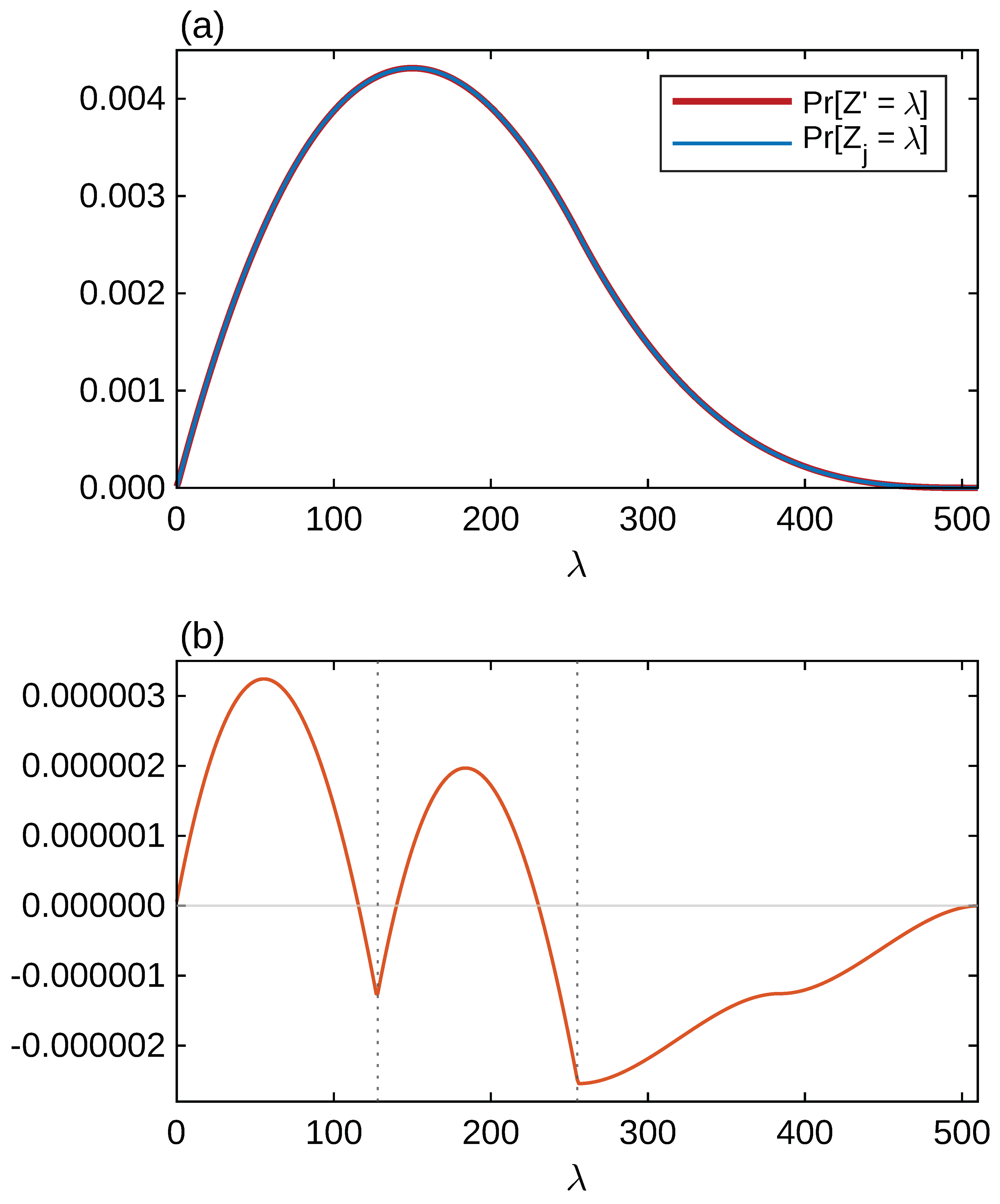

Table 1.
Deviation from uniform expectation across the byte alphabet.
| Range of v | Deviation |
|---|---|
| 0 | |
Table 2.
Probability of k byte disagreements in uniform byte pairs and float exponent byte pairs.
| k | |||
|---|---|---|---|
| 0 | |||
| 1 | |||
| 2 |
Table 3.
Reference values of the NPCR and UACI statistics under the uniform-byte and VSTL distributions.
Table 3.
Reference values of the NPCR and UACI statistics under the uniform-byte and VSTL distributions.
| Statistic | Unit | Uniform | VSTL | |
|---|---|---|---|---|
Table 4.
NPCR one-sided lower critical values under the VSTL and uniform-byte distributions.
| Reference mean | |||||||
|---|---|---|---|---|---|---|---|
| T | N | Uniform | VSTL | Uniform | VSTL | ||
| 100 | 5000 | ||||||
| 1000 | 50000 | ||||||
| 5000 | 250000 | ||||||
| 10000 | 500000 | ||||||
| 20000 | 1000000 | ||||||
| 50000 | 2500000 | ||||||
| 100000 | 5000000 | ||||||
Table 5.
UACI two-sided acceptance-interval bounds and under the uniform-byte and VSTL distributions.
Table 5.
UACI two-sided acceptance-interval bounds and under the uniform-byte and VSTL distributions.
| Reference mean | ||||||||||
|---|---|---|---|---|---|---|---|---|---|---|
| T | N | Uniform | VSTL | Uniform | VSTL | Uniform | VSTL | |||
| 100 | 5000 | |||||||||
| 1000 | 50000 | |||||||||
| 5000 | 250000 | |||||||||
| 10000 | 500000 | |||||||||
| 20000 | 1000000 | |||||||||
| 50000 | 2500000 | |||||||||
| 100000 | 5000000 | |||||||||
Disclaimer/Publisher’s Note: The statements, opinions and data contained in all publications are solely those of the individual author(s) and contributor(s) and not of MDPI and/or the editor(s). MDPI and/or the editor(s) disclaim responsibility for any injury to people or property resulting from any ideas, methods, instructions or products referred to in the content. |
© 2026 by the authors. Licensee MDPI, Basel, Switzerland. This article is an open access article distributed under the terms and conditions of the Creative Commons Attribution (CC BY) license (http://creativecommons.org/licenses/by/4.0/).
Copyright: This open access article is published under a Creative Commons CC BY 4.0 license, which permit the free download, distribution, and reuse, provided that the author and preprint are cited in any reuse.


