
Submitted:
20 June 2026
Posted:
23 June 2026
You are already at the latest version
Abstract
Reserved compute capacity is increasingly tradable amid surging AI-infrastructure investment: in large wholesale blocks and, more recently, through exchange-listed and cleared instruments. Yet pricing a compute capacity contract — a defaultable claim on a non-storable good that obsolesces on a known hardware cadence, sold by issuers that may fail in structurally distinct ways — still falls in the gap between standard commodity and credit finance. We develop a single-issuer pricing framework for this emerging asset class, adapting reduced-form credit intensity and F¨ollmer–Schweizer hedging to its defining features. The framework is closed-form under affine intensity and is exercised on an H100 forward through the H100→B200 transition.
Keywords:
compute capacity contracts
; GPU pricing
; defaultable claims
; commodity finance
; non-storable underlying
; lifecycle obsolescence
1. Introduction
Tradeable claims on future compute capacity are emerging at institutional scale: multi-billion-dollar wholesale transfers are disclosed (e.g., xAI [1]; Core Scientific, Inc. [2]; Hut 8 Corp. [3]; Applied Digital Corporation [4]; S&P Global Market Intelligence [5]); three regulated venues have launched cleared GPU-rental derivatives within six months (CME Group and Silicon Data [6]; Intercontinental Exchange [7]; Architect Financial Technologies [8]), cash-settled against an index with no issuer to deliver or default; and exchange-listed reservations trade alongside 24/7 DePIN secondary markets and partially-transferable hyperscaler reservations (Compute Exchange [9]; Amazon Web Services [10]). Valuation demand is rising, yet standard models miss two features that leave the market incomplete: multi-modal issuer non-performance and hardware obsolescence are jumps no traded instrument spans, so no unique arbitrage price exists. This paper proposes an issuer-agnostic pricing framework for the compute capacity contract, applied to a single defaultable issuer, its type entering only through calibrated inputs.
We price the compute capacity contract as a defaultable claim on a commodity forward. The market is incomplete, so we price and hedge by local risk-minimization under the minimal martingale measure (Section 6; Föllmer and Sondermann [11]; Föllmer and Schweizer [12]; Biagini and Cretarola [13]; Bielecki et al. [14]), which leaves the unspanned residual unpriced. Hardware obsolescence is the distinctive feature of the compute capacity contract: unlike a conventional commodity, the delivered good loses value as each successor generation ships. Obsolescence follows each manufacturer’s roadmap rather than a common schedule, so depreciation is a roadmap-anchored lifecycle process, not a fitted stationary rate. We adopt Cox reduced-form credit-intensity (Lando [15]; Duffie et al. [16]) with intensities affine in the state — the leading-order (linearization) specification that keeps pricing closed-form and calibratable from sparse data — and one discrete lifecycle Markov chain governs a single depreciation that enters both branches: its rate is the commodity drift (Section 4), and its accumulated depth the loading on the bankruptcy intensity ((11)), so obsolescence raises default risk exactly as it erodes value. Here g is the hardware grade vector, taken as an exogenous parameter (Section 2). The credit–value coupling is then structural and roadmap-pinned, fixed ex ante from the lifecycle rather than calibrated as a free parameter (cf. Hull and White [17]; Capponi et al. [18]; Frye [19]; Brigo et al. [20]). For a single issuer the level of this loading is set by the issuer’s own credit spread, while its variation across lifecycle states follows the roadmap depth ratio; cross-issuer exposure heterogeneity, through architecture-concentration and common-shock-clustering channels (diversified-cloud to grade-concentrated issuers), is the subject of the multi-issuer companion (Cao and Huang [21]). The nearest existing work prices compute as a good (commodity-finance and derivatives pricing, e.g., the inference-token futures of Xing [22]; the cleared index venues above), not a bilateral claim on a defaultable issuer with obsolescence as a joint driver. The framework fills that role, valuing the single-name, deliverable contract that actually transacts: a fair-value and credit-adjustment reference on top of the cleared index.
In this paper, we condition on the observed spot ; its endogenous dynamics lie outside scope. We likewise exclude the non-transferable limit, in which the tradeability friction diverges (Section 3).
2. The Compute Capacity Contract
The unit of analysis is the compute capacity contract: a contractual right entitling the holder to one unit of compute capacity at a specified hardware configuration from a specified issuer during a specified delivery window. The capacity-unit is most commonly one GPU-instance-hour but the framework applies equally to TPU-hours, Trainium-hours, Ascend-hours, and other architecture variants. Settlement may be token-based, database-recorded, or paper-based.
Definition 1
(Compute capacity contract). A compute capacity contract is a tuple where i is the issuer, g is the grade vector specifying the hardware configuration, T is the delivery period, is the settlement mechanism, and V is the value of the holder’s entitlement. The contract entitles the holder to one unit of compute capacity at grade g from issuer i during T, subject to issuer i’s SLA and continuity.
The grade g is a multi-dimensional vector taken as exogenous, in the standard commodity-finance treatment of grade as an industry-defined attribute (Tvedt [23]; Koekebakker et al. [24]). Table 1 catalogs the dimensions used in this paper; architecture family and generation set the lifecycle state of Section 4.
3. Two-Channel Pricing
A compute capacity contract is structurally a defaultable claim: the payoff depends jointly on issuer continuity (a credit-branch question) and on the value of the delivered capacity-unit at delivery (a commodity-branch question). Pricing therefore needs both machineries layered through a common pricing equation. We fix a single issuer throughout this paper and suppress the issuer subscript i on all symbols, restoring named subscripts only for the cross-sectional comparison of Section 7. Here, denotes the time-t forward price for delivery at T of one grade-g capacity-unit from the issuer — a defaultable claim whose delivery is contingent on issuer survival and SLA performance. We model on a filtered probability space satisfying the usual conditions, where is the physical (real-world) measure — under which the spot, default, and lifecycle dynamics evolve and are calibrated — and is the market filtration to which all processes are adapted. We price under a measure equivalent to . Compute markets are radically incomplete: the default time , recovery, and operational loss are not spanned by the tradeable spot , so no self-financing spot position replicates the claim and the equivalent martingale measure is not unique. We take to be the minimal martingale measure (MMM) of Föllmer and Schweizer [12], extended to defaultable claims by Biagini and Cretarola [13]: it prices the spanned commodity risk by no-arbitrage and assigns zero risk premium to the orthogonal, unhedgeable residual (default timing, recovery, operational loss), which the Föllmer–Schweizer local-risk-minimizing decomposition — the hedging counterpart of the MMM, developed in Section 6 — isolates as . This is a convention, not a no-arbitrage consequence: risk-averse pricing (e.g., minimal-entropy or utility-indifference) would load a positive premium on that residual, an out-of-model add-on. The affine specification of Section 6 satisfies the Biagini–Cretarola structure condition under which the MMM is well-defined.
Derivation.
Fix the trade time . Let denote the terminal failure stopping time (specified in Section 5), and let denote the realized time-T market value per delivered capacity-unit. The terminal event partitions paths: delivers capacity at T; settles via cause-conditional recovery; operational losses accumulate throughout the survival period. We take to be a doubly-stochastic (Cox) default time (Lando [15]; Duffie and Singleton [25]): the first instant an affine intensity crosses an independent unit-exponential threshold. This makes totally inaccessible with an affine hazard (the closed-form survival of Section 6) and satisfies the H-hypothesis (Bielecki and Rutkowski [26]), so the survival indicator and delivered value factorize conditional on the factor path, their unconditional covariance carried by the correction below. Setting
the three streams collapse to the pricing equation
where is the risk-free discount factor; in the recovery term , the face value V is fixed (the contract’s purchase price, Definition 1) and the recovery rate is cause-conditional — it equals the rate of whichever cause ends the contract, resolved over causes in Section 5, (9); is the operational counting process, and is the per-event net loss after SLA-credit recoveries. The spot–credit covariance
arises because the intensity and the spot share and the lifecycle state . Conditional independence is the corner (credit factors orthogonal to the spot), where the delivery term reduces to the familiar product ; in general is given in closed form in Section 6; as a price adjustment it scales with the default intensity, subdominant for investment-grade names and leading in the distressed regime (Section 7). Equation (1) is the framework’s centerpiece; its blocks are developed in turn: the cost-of-carry and its lifecycle drift (Section 4), the two-mode credit terms (Section 5), their affine form, lifecycle coupling, and -transform (Section 6), and the H100 calibration (Section 7).
Relation to CVA.
The credit adjustment is a unilateral credit valuation adjustment ( the exposure, the loss given default, the spot–credit covariance correction; Hull and White [17]; Brigo et al. [20]; Ballotta et al. [27]; Ghamami and Goldberg [28]; Brigo et al. [29]; Gregory [30]), but three features take it beyond the standard construction. The exposure is a non-storable, obsolescing commodity forward (Section 4), not a hedgeable mark-to-market taken as given. The credit–value coupling is structural and physical: the lifecycle chain (11) couples exposure and hazard — right-way on delivery, wrong-way on recovery — through hardware obsolescence itself, not a fitted correlation; unlike policy-driven firm-value stranding (Battiston et al. [31]), the shared driver is the asset’s own technology cycle. And the exposure is unspanned, priced by local risk-minimization under the MMM (Section 6) rather than by replication.
Cost-of-carry form of .
The survival-conditional forward admits the cost-of-carry exponential
where r is the risk-free rate, q is a convenience yield (below), u is the tradeability friction (below), and is the lifecycle-state-dependent technology drift (Section 4). A discrete event-premium factor aggregating governance and priority-access premia is typically () for single-issuer pricing and is omitted here.
Carry wedges q and u.
The exponent (2) also carries a convenience yield q, the Kaldor–Working–Brennan value of holding a reserved claim rather than inventory (Kaldor [32]; Brennan [33]; Gibson and Schwartz [34]; non-storable adaptation: Lucia and Schwartz [35]; Cartea and Figueroa [36]; Davis [37]; Bessembinder and Lemmon [38]; Routledge et al. [39]), and a tradeability friction u, the per-unit-time cost of reselling the claim: on liquid tiers, divergent () for non-transferable contracts, where cash-and-carry breaks and (1) is indicative rather than arbitrage-enforced. Both are secondary here. Spot and forward pin only the net exponent , so we fix ex ante from the roadmap (the load-bearing term, which then cannot absorb the others) and, on the transferable marketplace tier, set and fold q (financing roughly offsets it), leaving as the operative carry.
Grade-vector channels.
The grade g enters (1)–(2) through three distinct channels: the spot reference , the lifecycle-state drift via the state space of Section 4, and the face value V of Section 5 (the grade-specific purchase price). Cross-grade substitution operates through workload re-architecture, not a price discount, so a deliverable-substitute approximation overstates inter-grade fungibility; cross-grade no-arbitrage is a multi-grade question beyond this single-grade treatment.
4. Lifecycle States and Roadmap-Timed Transitions
This section develops the lifecycle technology-drift in the commodity forward of (1). Compute productivity moves through a discrete generational lifecycle (cf. Ma [40] on obsolescence and firm value), so a forward spanning a transition cannot be priced with constant drift. We make state-dependent, , over a compact state space restricted to the obsolescence-driven phases at or past a successor’s launch, where depreciation is structurally identifiable from roadmap cadence (Table 2). A current-generation grade with no announced successor is priced at observed spot with a low demand-dominated baseline outside the space, entering only at successor launch: the framework prices the obsolescence-driven shape, not the demand-driven level.
Definition 2
(Lifecycle state space). Within each architecture family, the lifecycle state space is the ordered set of obsolescence-driven regimes: mid-life (M, the post-launch depreciation cliff), commodity (C, legacy with moderate decelerating depreciation), and obsolete (O, drifting to a salvage floor), the three post-successor phases (Figure 1); the pre-successor phases (pre-launch, premium, mainstream) are demand-driven and form the exogenous frontier baseline outside . For grade g at time t, the state is observable from market signals; transitions proceed forward only, with ambiguous assignments handled probabilistically through the transition hazard (3).
Transition dynamics.
Transitions are partly deterministic (manufacturer roadmap cadence) and partly stochastic (timing slippage, demand shifts, supply-chain disruption), modeled through a probit hazard: the trigger is a scheduled event with a central expected date and roughly symmetric jitter , which a memoryless exponential (modal transition at ) cannot represent. For each transition , with expected transition time and timing uncertainty , the probability that grade g remains in state at time given entry at is
the survival function under a probit hazard, with the standard normal cumulative distribution function. The state distribution (the occupation probability, ) follows by iterating (3) along the sequential chain ; combining with the state-dependent drift gives the state-conditional mixture form
where is (1) evaluated with the within-state drift and within-state spot reference , the sum running over . Entry into M is set by the successor’s observed launch date; the two transitions within carry the roadmap-cadence anchors of Table 3 (V100/A100/H100 patterns, IntuitionLabs [42]).
Dual role across branches.
drives both branches of (1): commodity via the drift in (2), and credit via an obsolescence depth in the bankruptcy intensity (Section 6), the flow and the stock of one process. Obsolescence is set by performance-per-watt against the frontier: each generation improves efficiency per unit compute by roughly 2– on a near-annual cadence, and because power dominates datacenter operating cost, an older grade turns uneconomic for frontier work within 18–36 months [43]. We define as the normalized cumulative obsolescence of state , the stock whose instantaneous rate is : at the frontier and at the salvage floor. Writing for the drift accrued before state ( the sojourn of Table 3), the transient depths are the mid-sojourn fractions of the descent to the floor ,
the best single representative of the depth accrued while in each state. With /yr and sojourns yr, and , so and . Thus D is read from the roadmap, not chosen.
Anchoring obsolescence to perf-per-watt rather than to the rental price is deliberate: the H100 rental decline over the window was driven substantially by oversupply rather than obsolescence [41,44], while obsolescence proper redeploys capacity from training to inference, eroding revenue (price times utilization) and hardware collateral as the grade ages [45,46]. The perf-per-watt clock is roadmap-pinned and supply-free, so the credit–value coupling it induces is fixed ex ante. Because each drift in Table 2 is anchored to data disjoint from the grade’s own forward curve, the curve-implied recovered in Section 7 is an over-identifying restriction, and since D is the stock of the same check validates the depth.
5. Two-Mode Failure with Cause-Conditional Recovery
This section develops the credit blocks of (1) — the survival probability S and the loss terms and . These are the defaultable half of the defaultable-commodity framework, complementing the non-storable commodity branch . A bond’s credit risk reduces to a single binary default outcome. A compute capacity contract is exposed to two structurally distinct modes: operational failures (SLA breaches, partial-delivery shortfalls) partially recoverable through capped SLA credits, and terminal failures that end the contract, each cause carrying a distinct recovery profile (Table 4; competing-risks extension of reduced-form credit pricing, Bielecki and Rutkowski [26]). The 2022–2025 record supports this: specialized neoclouds operated continuously through H100 spot-rate volatility while mining-pivot operators experienced terminal failures (Compute North Holdings, Inc. [47]; Core Scientific, Inc. [48]); operational failures occurred in both groups without triggering terminal events.
Terminal failure with gated operational process.
Under , the terminal failure is a totally inaccessible stopping time with intensity adapted to the natural filtration. Under the doubly-stochastic Cox construction (Lando [15]; Bielecki and Rutkowski [26]), the survival probability admits
Operational failure events follow a Cox process with -intensity , where the indicator gates the intensity off after the terminal event: terminal is absorbing (the first occurrence ends the contract) while operational is recurrent (multiple events possible during the survival period). Each event produces net loss after capped SLA-credit recoveries (e.g., AWS Service Credits at 10–25% monthly fees, CoreWeave prorated refunds, and DePIN slashing bounded by staked pool). The expected operational loss takes the compensator form
We take the severity deterministic, so the operational stream needs no separate spot–credit correction; a spot-dependent severity would be quadratic in the state, handled as the recovery stream is in Remark 4.
Cause-conditional intensity decomposition.
Terminal failure resolves into competing causes. Each cause carries a first-jump intensity and a Cox stopping time —the first instant the integrated cause- intensity crosses an independent unit-exponential threshold, exactly as arises from (Section 3). Terminal failure is the earliest cause to fire, ; because the cause thresholds are independent, survival factorizes across causes and the intensities add,
with the cause- intensities conditionally independent given the state-factor path. Seven sub-causes organize the decomposition empirically, summarized in Table 4. The expected recovery in (1) sums over the cause that ends the contract, with cause-conditional recovery rate applied to the fixed face value V:
Remark 1
(Recovery of Face Value). The face value V is the contract’s purchase price (e.g., CoreWeave Order Form prepaid amount, AWS Capacity Blocks fee, and DePIN staked reference), priced under Recovery-of-Face-Value (Duffie [49]; cf. Jarrow and Turnbull [50]), distinct from the Recovery of Market Value of Duffie and Singleton [25]. RFV fits compute contracts: recovery clauses are denominated in fractions of purchase price, it has corporate-bond support (Berd et al. [51]; Casas Vivas [52]), and it avoids RMV’s “market value of an illiquid contract” issue.
Each loads on different state factors (bankruptcy on macro credit and idiosyncratic health, regulatory on jurisdictional exposure, force majeure on common shocks), and shares the macro factors of (the downturn-LGD channel), inducing –R correlation. The Biagini–Cretarola structure condition holds: the spot’s market price of risk has finite mean-variance tradeoff over the finite tenor, so the -density is a true martingale, and the default, recovery, and operational martingales are orthogonal to the spot Brownian under the Cox construction, leaving them unpriced.
Remark 2
(Wrong-way recovery covariance). Bankruptcy intensity and bankruptcy recovery share common-factor loadings:
where is the factor loading of on and is the factor covariance. Negative covariance signals wrong-way risk: bad states (high λ) coincide with low recoveries.
6. Affine Intensity, the Joint Spot–Credit Transform, and Lifecycle Coupling
This section casts the survival probability S of (1) in closed affine form, couples the lifecycle state to the bankruptcy intensity, and derives the Föllmer–Schweizer hedge. The cause-specific intensities and operational intensity are affine under , delivering closed-form survival via affine transform (Duffie et al. [16]). The affine form is the leading-order specification — the linearization of any smooth factor–intensity map, with the quadratic-affine extension (Cheng and Scaillet [53]) the principled next order, invoked only when curvature is identifiable — and it is the maximal class for which the pricing transform stays exponential-affine, so the survival, the spot–credit correction , and the hedge all inherit closed forms.
6.1. Intensity Dynamics and Closed-Form Survival
6.1.0.10. Factor state.
The joint state stacks common and idiosyncratic factors: , where captures supply, macro, infrastructure, and regulatory stress. Non-negative components follow CIR (Cox et al. [54]); naturally-signed components follow Vasicek (Vasicek [55]). Idiosyncratic follow CIR. The joint dynamics are affine,
with mean-reversion speeds , long-run means , and instantaneous covariance affine in the state: the Vasicek (Gaussian) components contribute the constant part , the CIR components the state-scaled part . The parameters are calibrated to the factor series (Section 7).
6.1.0.11. Affine intensity map.
The operational intensity and the terminal-cause intensities other than bankruptcy are affine in the state,
with intercepts , idiosyncratic loadings , and common-factor loadings constrained so the affine map preserves each ; the bankruptcy intensity carries an extra lifecycle term, defined next.
6.1.0.12. Lifecycle–bankruptcy coupling.
The state couples into the bankruptcy intensity through an additive covariate
with the cumulative-obsolescence depth of (5) (). Here is the issuer-specific lifecycle–credit loading, the sensitivity of the bankruptcy intensity to obsolescence depth. For a single issuer it is calibrated to the issuer’s own credit spread (Section 7). Lifecycle stress enters through revenue (old grades priced lower) and collateral (hardware-backed debt loses value as the fleet ages); it is additive to the macro and idiosyncratic baseline rather than an interaction with it, so downturn amplification lives in that baseline and the wrong-way recovery (Remark 4), not in the obsolescence term. Aggregating across via (8) yields an affine , with aggregate intercept and aggregate loading stacking on and on (zero on ); the lifecycle term is a state-conditional intercept carried by the regime system (23), not by .
6.1.0.13. Closed-form survival.
Under this specification, the survival probability (6) admits the closed-form exponential-affine expression
with and satisfying the Riccati system:
where are mean-reversion parameters and separate state-independent and state-dependent diffusion (the last term is component-wise). The system is the standard affine reduction — substitute the exponential-affine ansatz (12) into the Feynman–Kac equation for S and match coefficients in — with existence and uniqueness on multi-year tenors at typical calibrations from Duffie et al. [16]. Here (13) is the baseline (lifecycle-free) survival; the lifecycle-coupled form is the regime system (23), which with all couplings off (, no common shocks, a single cause) collapses to the Lando [15] closed-form. The operational loss (7) and the cause-conditional recovery (9) admit parallel exponential-affine forms via the same machinery; substitution into (1) yields tractable .
6.2. Hedging and the Joint Spot–Credit Transform
The last subsection fixed the credit side — the affine intensity, its lifecycle coupling, and the closed-form survival S that feeds the delivery term of (1). Now we turn to the spot–credit interaction, which surfaces at two orders: the Föllmer–Schweizer hedge ratio carries it at first order (an covariation beta), while the joint spot–credit transform delivers the level correction at second order (the factor ). One may thus price as if spot and credit were conditionally independent (the factorization of Section 3) but must not hedge that way.
6.2.0.14. Föllmer–Schweizer hedge ratio.
The Föllmer–Schweizer decomposition (Föllmer and Schweizer [12]) extended to defaultable claims by Biagini and Cretarola [13] writes the payoff as
is the predictable covariation ratio under the minimal martingale measure of Föllmer and Schweizer [12]; this ratio is the variance-minimizing hedge. The partial-derivative representation below holds for continuous-spot Markovian dynamics (the spot’s jump components feed ). Differentiating (1) under the cost-of-carry form, holding fixed at current state (),
The bracketed channel is spanned but not negligible — , , and the lifecycle state all co-move with , an sensitivity the hedge must carry. Keeping only the leading multiplicative term gives
The two reductions differ in status. The pieces (16) drops — the bracketed channel and the held-fixed spot-comovement of — are spanned, hence hedgeable: discarding them is hedge-ratio error, not irreducible risk, and “hedging as though spot and credit were independent” is exactly stopping at (16). What is genuinely unspanned is collected in — idiosyncratic intensity, Marshall–Olkin default jumps, lifecycle-transition jumps, and the unspanned part of recovery (wrong-way per Remark 2) — the irreducible incompleteness the minimal martingale measure leaves unpriced. Operationally the desk holds units of rental spot per unit of contract (survival times the carry ratio , each below one; the H100 value is calibrated in Section 7), carrying the bracketed channel up toward the full (15), and bears unhedged. The spanned correction is bounded by the state-conditional spread, across lifecycle states (a band, Section 7), with (16) the floor.
6.2.0.15. The joint spot–credit transform and the correction .
The transform is built from three ingredients — the object , the pricing measure, and an augmented state — assembled in Proposition 1 (with specialized to a single factor in Remark 3). The delivery term of (1) is the survival-weighted delivery
and the correction follow from the same affine machinery as the survival S above. The affine intensity map loads on the same that drive the spot , and the lifecycle state couples both branches through (11), so conditional independence () would require an orthogonality the framework’s own structure precludes.
6.2.0.16. The pricing measure under correlation.
The minimal martingale measure has density (Section 5), built only from the tradeable spot’s Brownian W and its market price of risk . By Girsanov, a common factor with acquires under the re-drift
with the factor’s mean-reversion rate and the spot–factor correlation (distinct from the continuity-premium ratio ); the CIR components carry the analogous essentially-affine adjustment (Duffee [56]). The same that breaks conditional independence sets how much of the spot’s risk premium the measure imputes to the credit factors, so covariance and re-drifting are one parameter: at the factors are orthogonal and unpriced, the regime Section 3, Section 4, Section 5, Section 6 and Section 7 operate in.
6.2.0.17. Augmented state.
Promote the log-spot to a state coordinate,
with -dynamics
so that recovers the cost-of-carry forward (2). Correlation enters only through the spot–factor diffusion blocks ; the intensity map does not load on (default responds to stress, not price level), and conditional independence (Section 3) is exactly .
Proposition 1
(Joint spot–credit transform). The delivery stream Ψ of (1) admits the exponential-affine form
where solve the Riccati system (13) on the augmented state (18), with the discount r added to the A-intercept, making it , under the single changed boundary condition
the unit vector on the log-spot coordinate, supplied by the payoff , and . The spot–credit covariance is carried by the quadratic term , with the augmented-state covariance: the -component of (equal to 1 at ) couples to the -components through the off-diagonals . When the block decouples and (19) factors as , the delivery term of (1) at the conditional-independence corner .
The proof is the affine reduction of Duffie et al. [16]: the ansatz (19) substituted into the Feynman–Kac equation for and matched in . The two transforms share the -equation of (13); only their terminal condition (20) differs.
Remark 3
(The conditional-independence correction as a single factor). For Gaussian factors, with is jointly Gaussian under and (19) reads
with the j-component of the aggregate loading . The correction is one scalar, multiplicative, and grows quadratically in tenor. Conditional independence is the null , a testable restriction: and the spot–factor correlations are estimable from the realized rental and credit series. Negative spot–credit comovement () makes , lifting the delivery stream above .
Remark 4
(Wrong-way recovery). The recovery stream carries the opposite-signed correction (terminal failures concentrate in low-spot states, the bankruptcy recovery itself wrong-way, Remark 2), but we leave uncorrected by design. The effect is sub-dominant in the investment-grade regime priced here (about of , Section 7), and anchoring to default-conditional recoveries (senior-unsecured averages and the 2022 cohort, both over actual defaults) already embeds the downturn-LGD, so the term is approximately wrong-way-correct without a separate factor. Pricing its dynamic factor covariance endogenously would require the quadratic-affine extension (Cheng and Scaillet [53]), available but unnecessary at the present data resolution.
The hedge ratio of (15) is the same correlation at first order: the level correction (21) is the covariance, while the bracketed channel of (15) is the covariation beta. Spot–credit dependence is thus priced in the hedge (first order) and in the level (second order), reconciling the conditional factorization of Section 3 with the first-order comovement established above.
6.3. Full Price and Exact Lifecycle Mixing
Two threads close the section: assembling the full price, and giving the lifecycle its exact, rather than mixture-approximated, treatment — the latter, (23) below, being the joint transform of Proposition 1 lifted to a Markov chain over regimes, inheriting its augmented-state machinery and adding only the generator coupling. First, every block of (1) is the same exponential-affine transform read off at a different rate and boundary — S at rate with ; at rate r with ; at rate with ; and as the matching default-timing and running integrals — so the full price assembles from this one object. Second, the mixture (4) weights these by the marginal state probabilities, dropping the path-coupling (the intensity carries over the whole path). Idealizing as a Markov chain with generator
restores it as the exact path treatment for the chain; the two sequential cadence rates are read from the roadmap, and the zero bottom row makes O absorbing, so once a grade obsolesces the coupling drops out. Write for the regime- transform coefficients, , and stack them as ; each solves
the obsolescence entering through and the last term the -row of the generator acting on the transform stack, ; solves the -equation of (13). This Markov idealization smooths the scheduled probit transitions (3), whose age-dependence is a further refinement negligible at the horizons priced here.
At the H100 horizon of Section 7 the system collapses to the marginal mixture (4): the transition falls past delivery ( mo against a 24-month tenor), so the grade occupies essentially one state over the whole tenor; the terminal occupancy that (4) weights by then already encodes the near-constant path, and the generator coupling — the only thing (23) adds beyond that marginal — is negligible. The full path treatment becomes first-order only when transitions fall inside the tenor (deep obsolescence, or the distressed regime).
7. Worked Example: H100 Forward Through Lifecycle Transition
We exercise the lifecycle states of Section 4 on an H100 forward spanning the H100 → B200 transition, anchoring all parameters to the Silicon Data H100 marketplace tier (the public series with the most consistent monthly methodology over the window). The rental market splits into a competitive marketplace tier (our anchor: the , transferable, arbitrage-enforced regime of Section 3), a higher neocloud tier, and an administered on-demand tier, distinct from the grade’s service tier (Section 2).
Setup.
At Q4 2024, H100 enters mid-life (M) as B200 begins volume shipping. Anchor spot: Silicon Data H100 2024 H2 marketplace median /hr (Silicon Data [41]); forward delivery Q4 2026 (24-month tenor). Drift anchors (exogenous, Table 2): /yr, /yr; the raw 2024 H2–2025 H2 endpoint ratio gives a ∼28%/yr realized rate (the V2 over-identifying check). Transition anchor: at mo, mo (IntuitionLabs [42]). State multiplier — the within-state spot scales as /hr. Scope: marketplace/cohort-median tiers, grade at or past mid-life.
Commodity-branch prediction.
The state distribution at mo is , . Within-state forwards /hr and /hr give the state-weighted commodity-branch forward /hr via (4).
Credit-branch contributions.
Anchoring to CoreWeave, a large-cap specialized neocloud (Fitch BB-/RR4 on the 9.25% 2030 senior unsecured notes, Z-spread bp; Fitch Ratings [57]; BondbloX [58]), implied /yr at (Moody’s senior-unsecured 5-year average, Moody’s Investors Service [59]). With /hr (RFV upper bound; actual prepaid amount typically 15–25% below spot, moving by ), ; /yr with /hr-equivalent (consistent with CoreWeave’s prorated-refund schedule and the AWS EC2 tier benchmark for moderate outages, Amazon Web Services [60]) yields /hr; bankruptcy recovery plus near-zero force-majeure/regulatory contributions give /hr (the recovery-of-face-value bound at the senior-unsecured , consistent with the rate used to imply ). The credit-adjusted forward is
Spot–credit correction.
Equation (24) reports the leading product (the term of (1)); we now evaluate the correction of Section 6. Calibrating the spot–credit inputs to the marketplace tier — realized rental log-volatility /yr, cumulative-hazard volatility over the 24-month tenor, and a negative spot–credit correlation (capacity glut and funding stress depress the rental and lift the intensity together) — the delivery-stream factor of (21) is , lifting from $1.295 to $1.304 (). The recovery stream moves the opposite way (Remark 4): a downturn-LGD haircut of order lowers from $0.12 to . The two nearly cancel, leaving to within , inside the credit-cohort band. The cancellation is structural: under negative spot–credit comovement the long gains on delivery (foregone deliveries fall in cheap-capacity states) and loses on recovery (those failures recover poorly). Conditional independence is therefore safe here demonstrably, not by assumption, but becomes leading and ceases to cancel in the distressed 2022 cohort, the regime of the multi-issuer companion (Cao and Huang [21]).
Parallel calibration: Applied Digital.
Substituting Applied Digital’s anchor (/yr, implied by its 9.25% senior secured notes due 2030 priced at 97 (∼580 bp) via at a secured recovery — distinct from the senior-unsecured used for CoreWeave; Applied Digital Corporation [61]) into (24): , , , /hr: Applied Digital’s higher intensity ( vs ) is more than offset by its secured recovery ( vs ), so it prices slightly above unsecured CoreWeave despite the wider spread — the framework netting recovery against intensity rather than reading the spread alone. The Föllmer–Schweizer cross-tier hedge (25) transfers via the same .
Lifecycle–credit coupling for the single issuer.
The CoreWeave spread pins the loading at mid-life through (11): against a diversified baseline (Table 5) and , the obsolescence increment is (), scaling by the depth ratio to at end-of-life, so rises from to as the grade ages. Carrying this rising intensity through the probit occupancy (3) (expected time-in-M of of 24 months, the transition lying beyond the tenor at mo) gives a cumulative hazard against at constant intensity, so S falls from to and by , within the credit-cohort band — the within-state intercept shift alone, the generator coupling of (23) being negligible at this horizon (Section 6). The within-issuer coupling is thus second-order at mid-life, becoming first-order only deep in obsolescence (older grades, longer tenors, or the distressed 2022 cohort), the regime of the multi-issuer companion (Cao and Huang [21]).
Per-issuer credit-spread sample.
A hedge book operates across the cohort. Table 5 samples named US-listed compute issuers with public credit data, plus the AAA/AA hyperscaler-parent benchmark.
Implied values use standard Z-spread for FINRA-traded bonds and Merton-style equity-implied default for equity-only issuers (Lando [15] for the reduced-form mapping). Cross-sectional spans (hyperscaler parents) to (Applied Digital), with Hut 8’s ring-fenced project notes a special investment-grade case at . At fixed unsecured recovery , sweeping ranges over around the CoreWeave-anchored $1.37 (higher reduces S but raises , partially offsetting); letting recovery instead track seniority makes the per-issuer forwards non-monotone in the spread (Table 6). The ∼19% cross-tier basis remains the dominant pricing-uncertainty channel.
Per-issuer forwards across the cohort.
Because the commodity branch , the face V, and the operational leg are issuer-agnostic (Section 5), each named issuer’s forward follows from its own intensity and seniority-implied recovery alone. The band is tight — spans $1.37–$1.45, about — so the commodity branch dominates and credit is a modest modifier. More telling, is not monotone in the spread: the lowest forwards are the unsecured neoclouds (CoreWeave $1.37, Nebius $1.38), not the highest-intensity miners (Applied Digital $1.43 at , Core Scientific $1.44 at ), whose secured recovery () more than offsets their intensity. The framework prices the recovery–intensity net, so reading off the spread while ignoring seniority would misrank the cohort.
In-scope universe and validations.
We fix the priced universe ex ante: transferable marketplace/cohort-median tiers (Silicon Data marketplace, DePIN, exchange-listed reservations) on NVIDIA GPUs spanning at most one generational transition, with hyperscaler on-demand (administered) and cross-tier comparisons out of scope, so the in-scope claims stand on their own. Figure 2 reports the realized-vs-predicted gaps. The two in-sample checks hold: the within-state path tracks the marketplace decline to 0.5% and 3% at 6 and 12 months (V1), and the endpoint-implied drift /yr runs ∼3pp hot of the roadmap-set 25% anchor (V2), a genuine realized-vs-anchor comparison rather than a tautology, since the anchor is not endpoint-fit. The clean out-of-sample test is cross-generational (V3): the H100-calibrated framework applied to A100 from Q1 2023 (anchor ∼$3.00/hr, Paperspace [62], 3-yr tenor) predicts ∼22.5%/yr and /hr against a realized $1.62/hr (AIMultiple [63]; 20.5%/yr), within 2pp without re-calibration. Out of scope, A100 on-demand declines ∼9pp slower (administered-tier inertia, V4, getdeploying [64]), and a two-generation V100 reach is directional only (V5, Amazon Web Services [65]). Table 7 consolidates the tests by evidentiary class.
Baselines: does the lifecycle machinery earn its complexity?
On the out-of-sample A100 test (V3), against the realized Q1 2026 cohort median $1.62/hr the lifecycle forward ($1.53, ) beats three naive predictors on the same anchor:
These are deliberately naive baselines — a no-depreciation null, the textbook cost-of-carry forward, and the single-rate practitioner default (the price-side analogue of hyperscalers’ straight-line GPU depreciation, here at the realized ∼25%/yr) — not the market benchmarks we turn to next. It roughly halves the error of the best foil (constant-decay) and dominates the level-based predictors by shifting drift across the transition the tenor spans; inside a single state it collapses to constant-decay, so the apparatus earns its complexity only on transition-spanning forwards.
Benchmarks: market forward curves and compute futures.
A genuine external benchmark for (24) now exists: vendor GPU forward curves to 36 months (Silicon Data [66]) and the cleared, cash-settled compute futures already noted (CME Group and Silicon Data [6]; Intercontinental Exchange [7]). These price the forward directly but reduced-form — a no-arbitrage term structure or a cleared quote on a spot index — a number, not a decomposition: no split of commodity from credit, no obsolescence transition, no issuer-specific default. The framework here is complementary and structural, supplying exactly those channels. Comparison must match the object: the index futures are credit-diversified, so they benchmark the commodity branch , whereas the single-issuer credit branch is validated separately by the per-issuer sample (Table 5); a tier-matched test of against the on-demand forward curve is the sharpest external check, available as these series mature.
Cross-tier comparison: SemiAnalysis forward index.
The SemiAnalysis H100 one-year forward index ( [67]) recorded $1.70/hr in October 2025, a ∼19% gap above the framework’s marketplace-tier $1.37/hr. Its index sits closer to Silicon Data’s neocloud tier ($2.99–$3.50/hr), consistent with tier-mix rather than framework error.
Föllmer–Schweizer cross-tier hedge ratio.
Let , so . The Föllmer–Schweizer covariation under gives
The Silicon Data tier series (Silicon Data [41]; months) puts and gives /$ (95% CI ), so , some below the naive . With significance marginal at (Newey–West widening the band to the opposite-sign region), we treat the basis-covariation channel as exploratory and prefer within-tier hedging (V1–V2), with a wide buffer (±6% or larger) where cross-tier exposure is unavoidable.
Sensitivity to lifecycle and recovery parameters.
Table 8 reports one-at-a-time perturbation sensitivity of to the four anchor parameters around base case.
The transition anchor dominates: a 24-month early transition compresses by ∼12%. is moderate (–) and small (–); recovery is – in the Moody’s bracket and across the realized compute-issuer range. Because is high-impact and thinly observed (the realized range rests on two 2022 data points), we treat it not as a constant but as a random recovery with the 2022-cohort spread (mean , support ), quoting with the resulting band. Transition-timing and recovery are the priority calibration targets; the rest are sub-dominant relative to the credit-cohort dispersion and ∼19% cross-tier basis.
8. Conclusions
The paper applies established credit-intensity and Föllmer–Schweizer hedging methodology to compute capacity contracts via two domain-specific structural choices. The shared discrete-state lifecycle Markov chain couples commodity drift and bankruptcy intensity; for a single issuer the obsolescence loading on the intensity is pinned by the issuer’s own credit spread and scales along the roadmap through the depth ratio of (11), with its cross-issuer heterogeneity deferred to the multi-issuer setting. The Föllmer–Schweizer cross-tier hedge ratio decomposes the cross-tier exposure into multiplicative-ratio and basis-covariation channels by the chain rule for product semimartingales; an exploratory regression on a short monthly panel (, marginal significance) suggests the basis-covariation magnitude lies below the multiplicative shortcut, short of a calibrated hedge ratio. Tractability is established by closed-form affine survival, the H100 example (within-tier gaps 0.5% and 3%), a naive benchmark on which the lifecycle-state model halves the best one-parameter foil’s error, the Applied Digital calibration, and an A100 cross-generation out-of-sample test within 2pp (plus a directional V100 reach). The framework prices forward-curve shape, not absolute spot level.
Use as a pricing reference.
The cleared venues price the commodity, credit-free; the bilateral contracts that transact carry a named issuer’s default and the hardware’s obsolescence, which no traded instrument spans. The framework supplies that single-name layer — the compute analogue of valuing a corporate bond off the curve plus an issuer spread. It can anchor fair value in a bilateral negotiation, supply a counterparty credit-valuation adjustment on a book of compute exposures (wrong-way included), mark balance-sheet and GPU-collateralized-loan positions to model, and frame a hedge against the index (the Föllmer–Schweizer ratio, with the unspanned credit residual flagged). It is a fair-value reference rather than a quote: the commodity leg is validated out-of-sample while the issuer overlay is calibrated to traded spreads, so an output is a band, not a point, and tightens as single-name forwards and the new compute futures (CME Group and Silicon Data [6]; Intercontinental Exchange [7]) mature.
References
- xAI. New Compute Partnership with Anthropic. xAI press release, 2026. Accessed June 2026.
- Core Scientific, Inc.. Core Scientific and CoreWeave Announce $1.2 Billion Expansion at Denton, TX Site. Core Scientific Investor Relations press release, 2025. Accessed June 2026.
- Hut 8 Corp.. Hut 8 Signs 15-Year, 245 MW AI Data Center Lease at River Bend Campus with Total Contract Value of $7.0 Billion. Hut 8 press release via PR Newswire, 2025. Accessed June 2026.
- Applied Digital Corporation. Applied Digital Announces New U.S.-Based High Investment-Grade Hyperscaler Tenant at Delta Forge 1, a 430 MW AI Factory Campus. Applied Digital Investor Relations press release, 2026. Accessed June 2026.
- S&P Global Market Intelligence. Bitcoin Miners Pivot to AI and HPC as Cryptocurrency Market Slumps. S&P Global Market Intelligence research note, 2026. Accessed June 2026.
- CME Group.; Silicon Data. CME Group and Silicon Data Partner to Launch First Compute Futures. CME Group press release, 2026. SDH100RT cash-settled GPU compute futures. Accessed June 2026.
- Intercontinental Exchange. ICE and Ornn to Launch GPU Compute Futures Contracts. ICE Investor Relations press release, 2026. OCPI cleared-futures complex (H100, H200, B200, RTX 5090). Accessed June 2026.
- Architect Financial Technologies. Architect Financial Technologies Partners with Compute Index Provider Ornn to Launch Exchange-Traded Futures on GPU and RAM Prices. PR Newswire press release, 2026. AX Exchange perpetual futures on the Ornn Computing Power Price Index. Accessed June 2026.
- Compute Exchange. NVIDIA H100 GPU Price in 2026: New, Refurbished, and Used. Compute Exchange research note, 2026. Accessed June 2026.
- Amazon Web Services. Amazon EC2 Capacity Blocks for ML can be shared across multiple accounts. AWS What’s New announcement, 2026. Accessed June 2026.
- Föllmer, H.; Sondermann, D. Hedging of non-redundant contingent claims. In Contributions to Mathematical Economics; Hildenbrand, W.; Mas-Colell, A., Eds.; North-Holland, 1986; pp. 205–223.
- Föllmer, H.; Schweizer, M. Hedging of contingent claims under incomplete information. In Applied Stochastic Analysis; Davis, M.H.A.; Elliott, R.J., Eds.; Gordon and Breach, 1991; pp. 389–414.
- Biagini, F.; Cretarola, A. Local risk-minimization for defaultable claims with recovery process. Applied Mathematics & Optimization 2012, 65, 293–314.
- Bielecki, T.R.; Jeanblanc, M.; Rutkowski, M. Hedging of defaultable claims. In Paris-Princeton Lectures on Mathematical Finance 2003; Springer, 2004; Vol. 1847, Lecture Notes in Mathematics, pp. 1–132.
- Lando, D. On Cox processes and credit risky securities. Review of Derivatives Research 1998, 2, 99–120.
- Duffie, D.; Pan, J.; Singleton, K.J. Transform analysis and asset pricing for affine jump-diffusions. Econometrica 2000, 68, 1343–1376.
- Hull, J.; White, A. CVA and wrong-way risk. Financial Analysts Journal 2012, 68, 58–69.
- Capponi, A.; Figueroa-López, J.E.; Nisen, J. Pricing and semimartingale representations of vulnerable contingent claims in regime-switching markets. Mathematical Finance 2014, 24, 250–288.
- Frye, J. Collateral damage. Risk 2000, 13, 91–94.
- Brigo, D.; Chourdakis, K.; Bakkar, I. Counterparty risk valuation for energy-commodities swaps: impact of volatilities and correlation. Energy Risk 2009.
- Cao, Z.; Huang, S. Pricing Portfolios of Compute Capacity Contracts: Cross-Issuer Dependence and Segment Classification. Working paper.
- Xing, Y. AI Token Futures Market: Commoditization of Compute and Derivatives Contract Design. arXiv preprint arXiv:2603.21690 2026.
- Tvedt, J. Valuation of VLCCs under income uncertainty. Maritime Policy & Management 1997, 24, 159–174.
- Koekebakker, S.; Adland, R.; Sødal, S. Pricing freight rate options. Transportation Research Part E: Logistics and Transportation Review 2007, 43, 535–548.
- Duffie, D.; Singleton, K.J. Modeling term structures of defaultable bonds. The Review of Financial Studies 1999, 12, 687–720.
- Bielecki, T.R.; Rutkowski, M. Credit Risk: Modeling, Valuation and Hedging; Springer Finance, Springer, 2002.
- Ballotta, L.; Fusai, G.; Marazzina, D. Integrated structural approach to credit value adjustment. European Journal of Operational Research 2019, 272, 1143–1157.
- Ghamami, S.; Goldberg, L.R. Stochastic intensity models of wrong way risk: wrong way CVA need not exceed independent CVA. Journal of Derivatives 2014, 21, 24–46.
- Brigo, D.; Morini, M.; Pallavicini, A. Counterparty Credit Risk, Collateral and Funding: With Pricing Cases for All Asset Classes; Wiley, 2013.
- Gregory, J. The xVA Challenge: Counterparty Credit Risk, Funding, Collateral, and Capital, 3rd ed.; Wiley, 2015.
- Battiston, S.; Mandel, A.; Monasterolo, I.; Roncoroni, A. Climate Credit Risk and Corporate Valuation. CEPR Discussion Paper 20239, Centre for Economic Policy Research, 2025.
- Kaldor, N. Speculation and Economic Stability. The Review of Economic Studies 1939, 7, 1–27.
- Brennan, M.J. The Supply of Storage. American Economic Review 1958, 48, 50–72.
- Gibson, R.; Schwartz, E.S. Stochastic convenience yield and the pricing of oil contingent claims. The Journal of Finance 1990, 45, 959–976.
- Lucia, J.J.; Schwartz, E.S. Electricity Prices and Power Derivatives: Evidence from the Nordic Power Exchange. Review of Derivatives Research 2002, 5, 5–50.
- Cartea, Á.; Figueroa, M.G. Pricing in electricity markets: A mean reverting jump diffusion model with seasonality. Applied Mathematical Finance 2005, 12, 313–335.
- Davis, M.H.A. Pricing weather derivatives by marginal value. Quantitative Finance 2001, 1, 305–308.
- Bessembinder, H.; Lemmon, M.L. Equilibrium pricing and optimal hedging in electricity forward markets. The Journal of Finance 2002, 57, 1347–1382.
- Routledge, B.R.; Seppi, D.J.; Spatt, C.S. Equilibrium forward curves for commodities. The Journal of Finance 2000, 55, 1297–1338.
- Ma, S. Technological Obsolescence. NBER Working Paper 29504, National Bureau of Economic Research, 2021.
- Silicon Data. H100 Rental Price Over Time (2023–2025): A Complete Market Analysis. Silicon Data market analysis, 2025. Tier-stratified median price series (hyperscaler / marketplace / neocloud) across 2023 H2–2025 H2. Accessed June 2026.
- IntuitionLabs. H100 Rental Prices Compared: $1.49–$6.98/hr Across 15+ Cloud Providers. IntuitionLabs cross-provider GPU pricing analysis (includes V100 and A100 cross-generation context), 2025. Accessed June 2026.
- CNBC. The Question Everyone in AI Is Asking: How Long Before a GPU Depreciates? CNBC, 2025. Per-generation efficiency roughly doubles to triples on a near-annual cadence; power-dominated TCO renders frontier-class grades uneconomic in 18–36 months; the GPU economic-life debate (Nadella, Burry). Accessed June 2026.
- Introl. GPU Cloud Prices Collapse: the H100 Rental Market, December 2025. Introl market report, 2025. H100 rental decline driven substantially by oversupply (300+ providers, AWS price cut) and a subsequent supply-tightening rebound, a market transition distinct from obsolescence. Accessed June 2026.
- WhiteFiber. Understanding the GPU Lifecycle. WhiteFiber technical note, 2025. GPU redeployment across training, inference, and infrastructure tiers; both rental price and utilization decline with grade age. Accessed June 2026.
- Stanley Laman. Why GPU Useful Life Is the Most Misunderstood Variable in AI Economics. Signals and Noise, 2025. Hardware-collateralized debt is under-collateralized when economic life (∼2–3yr) falls short of underwritten life (∼5–6yr); salvage erosion triggers covenants. Accessed June 2026.
- Compute North Holdings, Inc.. Voluntary Petition for Relief Under Chapter 11 of the Bankruptcy Code. United States Bankruptcy Court, Southern District of Texas (Houston Division), Case No. 22-90273, filed 22 September 2022, 2022. Accessed June 2026.
- Core Scientific, Inc.. Voluntary Petition for Relief Under Chapter 11 of the Bankruptcy Code. United States Bankruptcy Court, Southern District of Texas (Houston Division), Case No. 22-90341, filed 21 December 2022, 2022. Emerged January 2024. Accessed June 2026.
- Duffie, D. Defaultable Term Structure Models with Fractional Recovery of Par. Working paper, Graduate School of Business, Stanford University, 1998.
- Jarrow, R.A.; Turnbull, S.M. Pricing derivatives on financial securities subject to credit risk. The Journal of Finance 1995, 50, 53–85.
- Berd, A.M.; Mashal, R.; Wang, P. Defining, Estimating and Using Credit Term Structures. Working paper; arXiv:0912.4609.
- Casas Vivas, A. Fractional Recovery of Face Value in Sovereign Bond Markets. SSRN Working Paper 4892668.
- Cheng, P.; Scaillet, O. Linear-quadratic jump-diffusion modeling. Mathematical Finance 2007, 17, 575–598.
- Cox, J.C.; Ingersoll, J.E.; Ross, S.A. A theory of the term structure of interest rates. Econometrica 1985, 53, 385–407.
- Vasicek, O. An equilibrium characterization of the term structure. Journal of Financial Economics 1977, 5, 177–188.
- Duffee, G.R. Term premia and interest rate forecasts in affine models. The Journal of Finance 2002, 57, 405–443.
- Fitch Ratings. Fitch Awards First-Time BB- Rating to CoreWeave; Senior Unsecured Notes Rated BB-/RR4. Fitch Ratings press release, May 19, 2025, 2025. Issuer Default Rating BB- with positive outlook; $1.5B senior unsecured notes rated BB-/RR4 (31-50% expected recovery). Accessed June 2026.
- BondbloX. CoreWeave 9.25% Senior Unsecured Notes due 2030. BondbloX bond market data, 2026. Z-spread 454.1 bp, YTM 8.65% (secondary market). Accessed June 2026.
- Moody’s Investors Service. Annual Default Study. Moody’s Default and Recovery Database, 2025. Senior-unsecured 5-year average recovery 35.6 cents/dollar (ending June 2025). Accessed June 2026.
- Amazon Web Services. Amazon EC2 Service Level Agreement. AWS EC2 SLA, 2026. Tier structure: 10% credit (<99.99% uptime), 30% credit (<99%), 100% credit (<95%). Accessed June 2026.
- Applied Digital Corporation. Applied Digital Announces Pricing of $2.35 Billion of Senior Secured Notes. Applied Digital Investor Relations press release, 2025. 9.250% senior secured notes due 15 December 2030, issued by APLD ComputeCo LLC at 97% of par; $2.35 billion aggregate principal. Accessed June 2026.
- Paperspace. GPU Cloud Pricing Comparison. Paperspace cross-provider A100/V100 pricing comparison, 2023. Accessed June 2026.
- AIMultiple. Cloud GPU Rental Price Index. AIMultiple research aggregator (monthly snapshots, V100/A100/H100 cohort medians, 2024–2026), 2026. Accessed June 2026.
- getdeploying. NVIDIA A100 Cloud Pricing. getdeploying.com cross-provider GPU pricing aggregator (162 on-demand listings, mid-2026), 2026. Accessed June 2026.
- Amazon Web Services. New Amazon EC2 Instances with Up to 8 NVIDIA Tesla V100 GPUs (P3). AWS News Blog, 2017. p3.2xlarge (1x V100) on-demand $3.06/hr at launch. Accessed June 2026.
- Silicon Data. Silicon Data Unveils First GPU Forward Curve. Silicon Data news room, 2026. No-arbitrage implied-forward on-demand rental term structure to 36 months; normalized for spec, interconnect, and region. Accessed June 2026.
- SemiAnalysis. H100 GPU 1-Year Rental Price Index. SemiAnalysis pricing dataset, 2025–2026. Accessed June 2026.
Figure 1.
Three obsolescence-driven lifecycle states for a hardware grade g. The grade enters at mid-life when its successor launches (dashed: the pre-successor frontier period is an exogenous, demand-dominated baseline outside the state space) and transitions forward on publicly announced roadmap events. Within-state drifts decelerate toward a salvage floor; anchors in Table 2, calibrated values in the H100 example of Section 7.
Figure 1.
Three obsolescence-driven lifecycle states for a hardware grade g. The grade enters at mid-life when its successor launches (dashed: the pre-successor frontier period is an exogenous, demand-dominated baseline outside the state space) and transitions forward on publicly announced roadmap events. Within-state drifts decelerate toward a salvage floor; anchors in Table 2, calibrated values in the H100 example of Section 7.

Figure 2.
Data flow for the H100 worked example. Green: empirical sources with framework-symbol mappings; blue: framework outputs; orange: validations with realized-vs-predicted gaps. Within-tier and cross-generation validations (V1, V2, V3) achieve gaps of 0.5–3%; cross-tier vs SemiAnalysis exhibits the expected tier-attributable gap.
Figure 2.
Data flow for the H100 worked example. Green: empirical sources with framework-symbol mappings; blue: framework outputs; orange: validations with realized-vs-predicted gaps. Within-tier and cross-generation validations (V1, V2, V3) achieve gaps of 0.5–3%; cross-tier vs SemiAnalysis exhibits the expected tier-attributable gap.
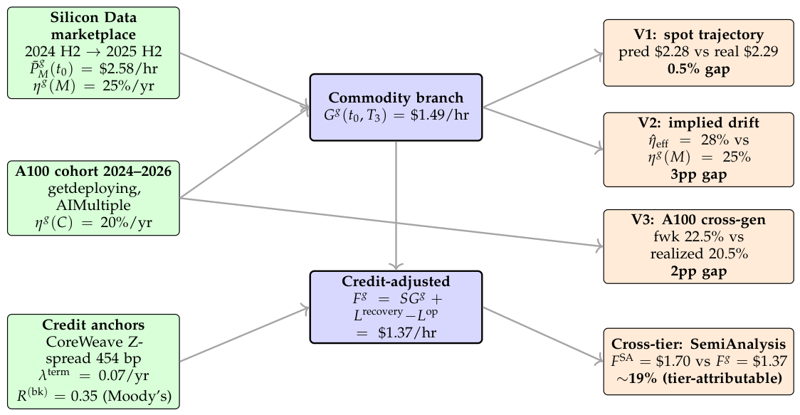

Table 1.
Grade-vector dimensions used in single-issuer pricing.
| Dimension | Illustrative values | Pricing relevance |
|---|---|---|
| Architecture family | NVIDIA Hopper/Blackwell, Google TPU, AWS Trainium, Huawei Ascend, AMD Instinct | First-order; sets the lifecycle states |
| Generation / model | H100, H200, B100, B200, B300, TPU v5p, Trainium 2 | First-order; within family, fixes the current lifecycle state |
| Interconnect | Within-node NVLink, cross-node InfiniBand or Ethernet | First-order for multi-node training workloads |
| Service tier | Bare-metal, managed-service, full-SLA | Often first-order; managed-service trades at 2–3× bare-metal |
Table 2.
Within-state technology-drift anchors, each fixed from a source independent of the issuer’s own forward curve, so the curve-implied drift recovered in Section 7 (Validation 2) is an over-identifying check rather than the calibration input (sources: SEC 10-Ks for accounting life, NVIDIA datasheets for performance-per-dollar, Silicon Data [41] for the rental decline, resale trackers for the obsolete floor). The obsolete state carries the least precise anchor and is not entered within tenor by the worked example.
Table 2.
Within-state technology-drift anchors, each fixed from a source independent of the issuer’s own forward curve, so the curve-implied drift recovered in Section 7 (Validation 2) is an over-identifying check rather than the calibration input (sources: SEC 10-Ks for accounting life, NVIDIA datasheets for performance-per-dollar, Silicon Data [41] for the rental decline, resale trackers for the obsolete floor). The obsolete state carries the least precise anchor and is not entered within tenor by the worked example.
| State | Exogenous anchor (independent of the grade’s forward curve) | Strength | |
|---|---|---|---|
| mid-life M | /yr | generational perf-per-dollar; rental decline of the just-superseded grade | strong |
| commodity C | /yr | hyperscaler accounting useful life (5–6 yr book) | strong |
| obsolete O | /yr | used-hardware resale residual (decelerating to a floor) | indicative |
Table 3.
Transition anchors ( measured from entry into the originating state). Entry into M (successor launch) is observed; the pre-M frontier period is exogenous and not modelled within .
Table 3.
Transition anchors ( measured from entry into the originating state). Entry into M (successor launch) is observed; the pre-M frontier period is exogenous and not modelled within .
| Transition | Trigger (roadmap event) | ||
|---|---|---|---|
| successor reaches mainstream | 30 mo | 6 mo | |
| end-of-life / second successor | 24 mo | 6 mo |
Table 4.
Sub-causes and recovery regimes. Non-bankruptcy empirical anchors: force majeure (Texas grid 2021, Hurricane Beryl 2024; ); regulatory (US export controls 2022–2025; ); ecosystem (Terra/Luna 2022; ); acquisition (2024 DC-portfolio M&A; ).
Table 4.
Sub-causes and recovery regimes. Non-bankruptcy empirical anchors: force majeure (Texas grid 2021, Hurricane Beryl 2024; ); regulatory (US export controls 2022–2025; ); ecosystem (Terra/Luna 2022; ); acquisition (2024 DC-portfolio M&A; ).
| Cause | Mechanism | Recovery regime |
|---|---|---|
| Bankruptcy (bk) | Insolvency via revenue collapse, debt distress, capital-flight cascade | Stochastic estate distribution; , downturn-LGD correlated |
| Force majeure (fm) | Disaster, cyber attack, civil-authority order, sanctions equipment block, upstream grid collapse | by standard SLA exclusion |
| Regulatory shutdown (rs) | Export-control revocation, sanctions, agency-ordered termination | ; voided by government action |
| Acquisition · assumption (aa) | Acquirer assumes contract at original terms | via successor entity |
| Acquisition · repudiation (ar) | Acquirer declines; contract becomes residual claim | ; acquirer discretion, creditor priority |
| Ecosystem collapse (ec) | Issuer survives but supporting ecosystem ceases delivery | ; higher if distributed operators persist |
| Verifiability dispute (vd) | Issuer survives but SLA enforcement fails (measurement, arbitration) | Case-specific via dispute mechanism |
Table 5.
Per-issuer credit-anchor sample with public data sources (SEC EDGAR; FINRA TRACE; rating-agency press releases). CoreWeave provides the central single-name secondary-market anchor. †Hut 8’s anchor is its ring-fenced River Bend project-finance note (BBB-, bankruptcy-remote SPV backed by a hyperscaler-linked lease); its ∼0.003 intensity reflects that lease-backed structure and understates Hut 8 Corp parent and compute-delivery risk.
Table 5.
Per-issuer credit-anchor sample with public data sources (SEC EDGAR; FINRA TRACE; rating-agency press releases). CoreWeave provides the central single-name secondary-market anchor. †Hut 8’s anchor is its ring-fenced River Bend project-finance note (BBB-, bankruptcy-remote SPV backed by a hyperscaler-linked lease); its ∼0.003 intensity reflects that lease-backed structure and understates Hut 8 Corp parent and compute-delivery risk.
| Issuer | Credit anchor | Public source | |
|---|---|---|---|
| AWS, GCP, Azure | AAA/AA parent sr unsec | Issuer-parent benchmarks | 0.005–0.015 |
| CoreWeave | Fitch BB-/RR4; 9.25% 2030 Z-spread ∼454 bp | Fitch Ratings [57]; BondbloX [58]; TRACE | 0.07 |
| Nebius | Equity-implied via Merton | SEC 20-F/6-F; equity vol | 0.04–0.08 |
| Hut 8 | 6.192% sr secured 2042; BBB- (IG)† | PR; SEC; S&P/Fitch | ∼0.003 |
| Applied Digital | 9.25% sr secured 2030 at 97; ∼580 bp impl. | Applied Digital Corporation [61]; SEC 8-K; TRACE | 0.12–0.15 |
| Core Scientific(post-emergence) | 7.75% sr secured 2031; B+/S&P (2026) | SEC; S&P; TRACE | 0.08–0.13 |
Table 6.
Per-issuer credit-adjusted forward in $/hr, holding the commodity branch at , RFV face , and (all issuer-agnostic) and varying only intensity and seniority-implied recovery : , , . The are representative midpoints of Table 5; the spot–credit correction is negligible outside the distressed regime. Secured high-intensity issuers (Applied Digital, Core Scientific) price near the hyperscaler and project-finance names — recovery offsets intensity — above the unsecured neoclouds.
Table 6.
Per-issuer credit-adjusted forward in $/hr, holding the commodity branch at , RFV face , and (all issuer-agnostic) and varying only intensity and seniority-implied recovery : , , . The are representative midpoints of Table 5; the spot–credit correction is negligible outside the distressed regime. Secured high-intensity issuers (Applied Digital, Core Scientific) price near the hyperscaler and project-finance names — recovery offsets intensity — above the unsecured neoclouds.
| Issuer | Class | S | ||||
|---|---|---|---|---|---|---|
| AWS / GCP / Azure | Hyperscaler parent | 0.01 | 0.35 | 0.98 | 0.02 | 1.44 |
| Hut 8 (River Bend) | Project-finance (IG) | 0.003 | 0.55 | 0.99 | 0.01 | 1.45 |
| CoreWeave | Neocloud (unsec.) | 0.07 | 0.35 | 0.87 | 0.12 | 1.37 |
| Nebius | Neocloud (unsec.) | 0.06 | 0.35 | 0.89 | 0.10 | 1.38 |
| Core Scientific | Miner-pivot (sec.) | 0.10 | 0.55 | 0.82 | 0.26 | 1.44 |
| Applied Digital | Miner-pivot (sec.) | 0.13 | 0.55 | 0.77 | 0.33 | 1.43 |
Table 7.
Validation scorecard for the worked example. The three prediction tests (in-sample V1, over-identifying V2, out-of-sample V3) probe the commodity branch, which carries the bulk of the price; V3 — the H100-calibrated model applied to A100 without recalibration — is the clean out-of-sample check. The ablation confirms the lifecycle machinery beats the best naïve foil; the tier-basis row is a consistency check (it attributes a gap to tier-mix, not a prediction); recovery and the cross-tier hedge are low-power by construction (two realized defaults; an -month panel). The sharpest external check still to come — against the cleared CME/ICE futures strip, a credit-free index (CME Group and Silicon Data [6]; Intercontinental Exchange [7])—arrives as those contracts settle.
Table 7.
Validation scorecard for the worked example. The three prediction tests (in-sample V1, over-identifying V2, out-of-sample V3) probe the commodity branch, which carries the bulk of the price; V3 — the H100-calibrated model applied to A100 without recalibration — is the clean out-of-sample check. The ablation confirms the lifecycle machinery beats the best naïve foil; the tier-basis row is a consistency check (it attributes a gap to tier-mix, not a prediction); recovery and the cross-tier hedge are low-power by construction (two realized defaults; an -month panel). The sharpest external check still to come — against the cleared CME/ICE futures strip, a credit-free index (CME Group and Silicon Data [6]; Intercontinental Exchange [7])—arrives as those contracts settle.
| Quantity | Model | Benchmark / data | Result | Class |
|---|---|---|---|---|
| Spot path, H100 | Silicon Data marketplace | – @ 6/12 mo | in-sample (V1) | |
| Drift, H100 | anchor | endpoint-implied | 3 pp | over-identifying (V2) |
| Forward, A100 | () | realized () | / 2 pp | out-of-sample (V3) |
| vs. naïve foils | () | constant-decay () | halves error | ablation |
| Tier basis | marketplace | SemiAnalysis | ∼19% attributable | consistency |
| Recovery | 2022 cohort – | inside range | low power () | |
| Cross-tier hedge | tier series () | marginal sig. | exploratory |
Table 8.
One-at-a-time perturbation sensitivity of around base case (mo, mo, , ); /yr. Realized-compute range spans the 2022 cohort (Compute North ; Core Scientific via reorganization continuation; Compute North Holdings, Inc. [47]; Core Scientific, Inc. [48]).
| Parameter | Low | Base | High | low / high ($/hr) | Range vs base |
|---|---|---|---|---|---|
| (months) | 24 | 30 | 36 | $1.21 / $1.43 | / |
| (months) | 3 | 6 | 12 | $1.43 / $1.30 | / |
| 0.5 | 0.6 | 0.7 | $1.34 / $1.39 | / | |
| (Moody’s bracket) | 0.25 | 0.35 | 0.50 | $1.34 / $1.42 | / |
| (realized compute) | 0.15 | 0.35 | 1.00 | $1.31 / $1.59 | / |
Disclaimer/Publisher’s Note: The statements, opinions and data contained in all publications are solely those of the individual author(s) and contributor(s) and not of MDPI and/or the editor(s). MDPI and/or the editor(s) disclaim responsibility for any injury to people or property resulting from any ideas, methods, instructions or products referred to in the content. |
© 2026 by the authors. Licensee MDPI, Basel, Switzerland. This article is an open access article distributed under the terms and conditions of the Creative Commons Attribution (CC BY) license (http://creativecommons.org/licenses/by/4.0/).
Copyright: This open access article is published under a Creative Commons CC BY 4.0 license, which permit the free download, distribution, and reuse, provided that the author and preprint are cited in any reuse.


