Submitted:
21 June 2026
Posted:
23 June 2026
You are already at the latest version
Abstract
Machine learning (ML) and deep learning (DL) have made great improvements in classifying cancer, but there are problems that go past the basic difference between tumor and normal cells. Models trained on extensive datasets such as Clinical Proteomic Tumor Analysis Consortium (CPTAC) and The Cancer Genome Atlas (TCGA) demonstrate high accuracy in tumor detection. However, performance diminishes in clinically significant tasks such as molecular subtyping, stage and grade prediction, prognosis estimation, and tissue-of-origin identification. Evidence from various omics and imaging modalities establishes the data foundations of computational oncology and conceptualizes cancer classification as a hierarchical challenge characterized by diminishing predictive performance as biological complexity escalates. Biological signal strength has a bigger effect on performance than model architecture. Preprocessing steps, such as normalization, scaling, imputation, and batch correction, are recognized as significant factors influencing model outcomes, especially in heterogeneous datasets. Multimodal fusion strategies enhance robustness but yield minimal improvements in sensitivity owing to inadequate spatial-molecular alignment.Current methods have a basic sensitivity limit. Progress in clinically relevant prediction will depend on better data resolution, careful preprocessing, and strict validation, rather than more complex models. The following review examines each of these arguments in depth, from data foundations to hierarchical classification tasks that expose their limitations.
Keywords:
cancer classification
; machine learning
; deep learning
; multi-omics integration
; transcriptomics
; proteomics
; digital pathology
; radiomics
; multimodal learning
; tumor heterogeneity
; preprocessing
; class imbalance
; prognosis prediction
; tissue of origin
; TCGA
; CPTAC
; computational oncology
1. Introduction
Cancer is the second leading cause of mortality all over the world, with new cancer statistics reaching around 19.3 million, resulting in approximately 10 million deaths by 2020 (Chhikara and Parang). Recent advancements in High Throughput Omics and Deep Learning have altered the cancer detection paradigm. While tumor vs. normal classification has almost 100% accuracy, predicting diseases at early stages continues to be a constant challenge.
Established tumor data clearly exhibits specific molecular signatures, yet current medical scenarios require models to efficiently identify the specific grade (cellular differentiation) and stage, prognosis, subtyping to determine accurate mode of treatment (Noorbakhsh et al., 2020). Current methods are insensitive to biological data leading to late-stage cancer detection, which creates a challenge for early diagnosis due to tumor heterogenicity. (Wei et al., 2022; Wang et al., 2025). The integration of multi-omics data can further improve model accuracy for diagnosis and prognosis (Hsu et al., 2025).
This review examines the role of ML & DL in cancer classification beyond simple tumor vs normal detection.
- By surveying data foundations for model training by covering major omics data types (transcriptomics & proteomics), imaging inputs (radiology, digital pathology), single cell and clinical label structures.
- It also maps hierarchical nature of classification from binary models through molecular subtyping, stage & grade, prognosis to tissue of origin models.
- Major focuses on ML & DL architecture via ensemble, convolution for images, graph neural networks and generative models.
- Furthermore, it examines open challenges including label noise, cross cohort generalization & absence of benchmarking frameworks.
2. Data Foundations for Tumor Modeling
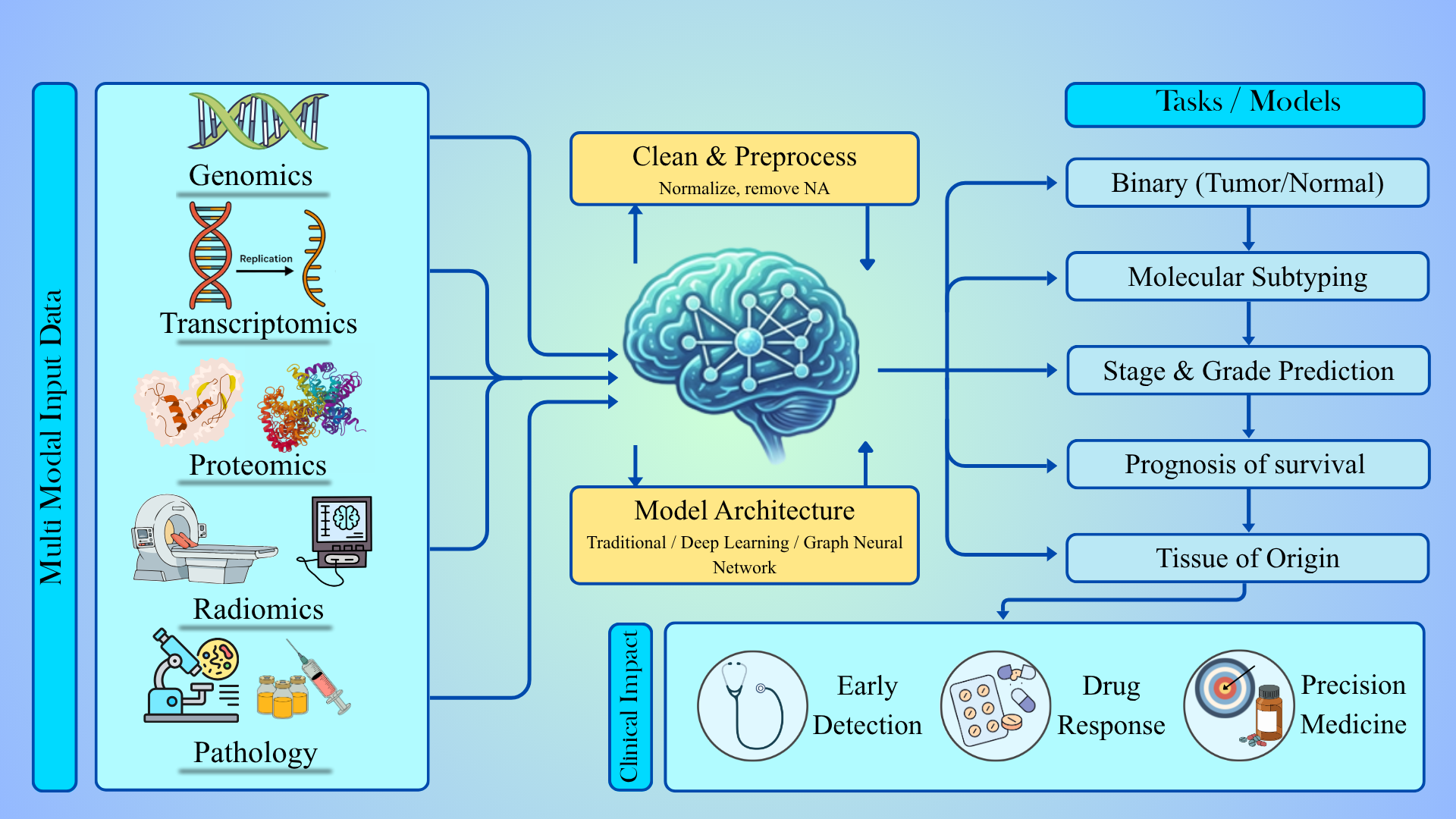
Robust tumor modelling depends on availability of large, well annotated datasets. This section talks about all of the omics modalities, imaging inputs, and clinical labels categorized based on malignant and non-malignant tissue samples. Integrating multi-omics such as genomics; transcriptomics; epigenomics; proteomics; and metabolomics provides significant advances in the understanding of the molecular basis of complex diseases including cancer. The overview of the foundations are represented in Figure 1.
2.1. Molecular Omics Data
Technologies now comprehensively identify and quantify molecules of a defined biological class within a tissue sample (Han et al., 2025). Each omics layer provides a different perspective as no single layer can adequately describe all aspects of tumor behaviour.
2.1.1. Transcriptomic
Transcriptome sequencing (aka RNA-seq) quantifies and identifies coding and non-coding RNAs (microRNAs, mRNAs, rRNAs, tRNAs, lncRNAs). It also discovers new transcripts in the sequence (Barbadikar, K. M. et. al. 2023).
The Cancer Genome Atlas (TCGA) (https://www.cancer.gov/ccg/research/genome-sequencing/tcga) project is one of the most extensive multi-omics analyses of cancer, with thousands of samples across more than 30 cancer types. It offers uniform sequencing & clinically annotated molecular modalities, making it an essential resource for tumor machine learning models (Hsu et al., 2025). RNA-seq can swiftly detect and measure rare and frequent transcripts, variants, novel transcripts, and non-coding RNAs from high and low-quality samples (Z. Wang et al., 2008). MicroRNA sequencing (miRNAseq) focuses on small RNAs, enabling the detection of specific short, noncoding RNAs (miRNAs). These genes are crucial in regulating various signaling pathways (Tomczak et al., 2015). However, TCGA has a relatively small number of matched normals compared to tumor samples across many cancer types. This affects statistical power and generalizability models.
To tackle this issue, the Genotype-Tissue Expression (GTEx) (https://gtexportal.org/home/) project offers RNA-seq profiles from non-diseased human tissues. Several studies have systematically integrated this data (Zeng et al., 2019; Tian et al., 2024a; C. Wang et al., 2023). Furthermore, The European Genome-phenome Archive (EGA) (https://ega-archive.org/) provides access to restricted transcriptomic datasets under limited access to safeguard patient privacy (Lappalainen et al., 2015).
In addition, platforms direct their resources towards curation and reuse of transcriptomic datasets. The Gene Expression Omnibus (GEO) (https://www.ncbi.nlm.nih.gov/geo/) and ArrayExpress function as a repository for both microarray-based & RNA-seq gene expression research across the global research community, making them vital resources for secondary transcriptomic analysis and meta-studies. Tools like UCSC Xena and cBioPortal offer harmonized, transcriptomic matrices derived from TCGA, ICGC along with visualization tools for ML workflow (J. Wang et al., 2025).
2.1.2. Proteomic Data Sources
Genomics and transcriptomic data capture mutational potential and transcriptional activity, respectively. Proteomics is one type of molecular information that directly shows the functional state of a cancer cell (Li et al. 2023). Protein abundance and post-translational modifications reflect the phenotype shown by the tumor (Bruno et al. 2025). Proteomic studies have shown that mRNA abundance can only explain a part of protein level variability in cancer which brings to notice the importance of proteomics study as an independent and supportive modality for computational tumor classification, including machine learning (Zhang et al., 2014; Mertins et al., 2016).
The growing role of proteomics in computational oncology is supported by large scale multi-omics platforms that systematically profile tumor biology across different molecular layers. The Clinical Proteomic Tumor Analysis Consortium (CPTAC) (https://gdc.cancer.gov/about-gdc/contributed-genomic-data-cancer-research/clinical-proteomic-tumor-analysis-consortium-cptac) (Lindgren et al., 2021) includes detailed grouping of tumors and their matched normal samples throughout multiple cancer types. The integration of proteomics, phosphoproteomics, transcriptomics and detailed clinical annotations (Zhang et al., 2014; Mertins et al., 2016) allows the investigation of how genomic alterations lead to changes at the protein level. In contrast, single-omics analysis captures molecular events that are isolated from each other. Integrating multi-omics features involves the study of cross-layer biological interactions, allowing proper analysis of tumor progression and heterogeneity. CPTAC uses standardized mass spectrometry workflows like tandem mass tag based (TMT based) pipelines, reducing inter-cohort technical variability (Mertins et al., 2016).
The CPTAC Python API offers CPTAC data tables in a uniform manner across tumor types, to enable repeatable and programmatic access to these datasets. By removing batch-specific preparation, this resource allows for direct interaction with ML processes. View the software documentation at https://paynelab.github.io/cptac/. View the GitHub repository at https://github.com/PayneLab/cptac (Lindgren et al. (2021)).
Proteomics datasets are classified into global proteomics and phosphoproteomics that can be used for tumor modelling with different modelling implications (Higgins et al., 2023). Global proteomics is used to measure steady-state protein abundance for tumor vs normal classification, subtype classification and biomarker discovery (Zhang et al., 2014; Mertins et al., 2016). On one hand where global proteomics captures broad abundance level changes, phosphoproteomics offers deeper insight into the dynamics of signaling activity and kinase mediated regulation. Phosphoproteomics identifies signaling pathways and kinase driven regulation. Even though phosphoproteomics data inherently demonstrates an increased sparsity and missingness, it provides a mechanistic insight (Jiang et al., 2024). Protein-level confirmation is important for finding biomarkers, according to studies combining transcriptomic feature selection with protein-level validation (Ning et al., 2024). The major proteomic data sources and their implications for machine learning tasks are summarized in Table 1.
One inherent limitation is the bulk nature of the data (Dent & Diamandis, 2022). CPTAC proteomics measures average protein abundance across heterogeneous cellular populations. Averaging can obscure cell type specific signals and spatial heterogeneity. Models report strong performance for tumor vs normal classification but reduced accuracy in identifying intermediate stages (Zhang et al., 2014; Mertins et al., 2016). Proteomics is effective in capturing functionally active disease states and its integration with spatially resolved and imaging based features can further increase the sensitivity for early stage and low-grade tumor characteristics. (Boys et al., 2023). This necessitates integrating spatially resolved modalities, such as histopathology images, to restore the contextual information lost in bulk measurements. All these observations point towards the importance of multi-omics integration, where these multi-omics modalities complement biological signals that cannot be fully represented by a single molecular layer alone.
2.1.3. Others
Genomics can generate huge amounts of data, primarily DNA sequence data from high throughput sequencing (e.g., Illumina, PacBio, Nanopore), variation data (including SNPs, InDels, CNVs, and structural variations) and gene annotations. The most appropriate data input is mutation signature of unique characteristics (Alharbi & Rashid, 2022). DNA methylation profiles from Illumina's 450K and EPIC arrays yield beta value matrices with between 450K and 850K CpG methylation data points collected per subject. These high-dimensional inputs are further used to identify methylation markers for prognosis but having high collinear data or nonlinear interactions in epigenome leads to substantial differences in model metrics (Yuan et al., 2023). Metabolomic profiling (using LC-MS/MS or NMR) generates real time measurements of small molecules. Apart from transcriptomics and proteomics, there is no standardized pan cancer metabolomic data repository equivalent to TCGA or CPTAC. (Alharbi & Rashid, 2022, Yuan et al., 2023). Some of the sources are detailed below in Table 2
While molecular omics data captures biological state at gene or protein level, it provides no information about organization of tissues. This is explored & addressed by imaging modalities.
2.2. Imaging & Radiomics Data Sources
Imaging data provides a unique insight compared to all other data types that contain molecular assays. Features include spatial organization, tissue architecture, and cellular morphology cannot be studied using bulk omics. WSIs are digitization of hematoxylin and eosin (H&E) stained tissue sections at subcellular resolution, producing gigapixel scale images that encode nuclear atypia, glandular stress and stromal composition. These features help pathologists determine stage and grade and are effective for training machine learning models. The structural complexity shown by WSIs has incentivized the development of DL architectures that have the ability to model long range spatial interactions.
Graph based and transformer based WSI models capture long range spatial dependencies not well captured in patch based convolutional approaches (Zheng et al., 2022). WSIs are label ambiguous. Diagnostic labels are assigned at the slide or patient level, but only part of the regions may contain differentiating pathological features. This labelling pattern is reason enough for development of weakly supervised and multiple instance learning (MIL) frameworks that learn differentiating regional patterns from slide level annotations.
Immunohistochemistry (IHC) based imaging provides information at the interface of molecular and morphological data. IHC data bridges the gap between proteomics by visualizing protein expressions wit.ch is demonstrated in Ning et al. (2024), where transcriptomic feature selection is followed by protein-level validation and subsequent machine learning on IHC images. IHC offers high biological specificity and interpretability, making these models suitable for binary diagnostic classification, while more complex prediction tasks benefit from integration with broader spatial or molecular modalities.
Imaging datasets are usually linked to genomic databases like TCGA and CPTAC. While standardized preprocessing pipelines are available for molecular data, they are lacking for imaging data. Just as proteomics data shows strong performance for coarse classification models but struggle with fine grained distinctions, the same is the case for imaging. This motivates multimodal integration, where the imaging data provides structural and spatial aspects of tumors and the omics data provides molecular specificity.
Spatial heterogeneity is important because changing immune infiltration levels influence clinical outcomes. Graph based WSI models take advantage of spatial relationships in the data, but they lack accuracy in stage and grade predictions, indicating that morphology alone does not capture the subtleties of progression. Variability in tissue processing creates batch effects, complicating harmonizing datasets and risking overfitting. Imaging datasets cannot be used interchangeably as differences in resolution, contrast, and patient demographic variables can have a significant impact upon the model's efficacy, indicating that a model's performance is fundamentally related to both its training data quality and its training data provenance (Zheng et al., 2022, Carrillo-Perez et al., 2023). Bulk imaging & molecular assays both lose fine details through averaging. Therein, spatial & single omics methods have merged to restore that resolution.
2.3. Spatial & Single Cell
What happens inside a tumor can differ wildly from one cell to another, yet bulk RNA-seq blurs these differences by combining signals from thousands of cells into one average. To see finer detail, single-cell methods capture activity within each individual cell instead. Meanwhile, spatial techniques preserve location-based patterns, mapping where specific genes turn on across tissue sections.
Single cell RNA aids in resolving tumor cells by measuring the individual gene expression of each cell. However, scRNA-seq has limitations: spatial information about tissue architecture is not preserved, therefore, it is not possible to understand how cells are organized or communicate with one another within the intact architecture of the tissue itself (Xiao et al., 2024). Most publicly available scRNA-seq cancer datasets are deposited at GEO, HCA Data Portal and the Single Cell Portal at the Broad Institute, and separate cohorts of matched scRNA-seq and clinical data are available through the Human Tumor Atlas Network (HTAN) for select cohorts within the Clinical Proteomic Tumor Analysis Consortium (CPTAC). De Zuani et al. (2024) performed an integrative analysis of scRNA-seq data in 25 treatment-naïve patients with NON-Small Cell Lung Carcinoma, approximately 900,000 single cells were profiled. They found inversely correlated numbers of anti-inflammatory macrophages and NK/T cells, difference in co expression of inhibitors between carcinoma subtypes. These are all findings that were not discerned from traditional bulk RNA-seq data in these same patients
Spatial Transcriptomics. First is the sequencing-based approaches (10x Visium, Stereo-seq, Slide-seqV2) which sequence RNA from capture spots & report expression at tissue coordinates. Second is the imaging-based approaches (MERFISH, STARmap PLUS) which use fluorescence hybridization to detect a gene panel to achieve precision. Resolution and sensitivity trade-offs associated with these two types of technology differ significantly from each other (Hu et al., 2023).
All sequencing platforms have a major technical restriction, sometimes the average of 80% of data being 0s. It is challenging to identify whether a measured zero represents a true biological absence from the sample as compared to one created by averaging (Sarkar et al., 2024). To address this, several deconvolution methods have been created to establish cellular composition.
2.4. Clinical Labels and Biological Meaning
Various labels are required to aid in categorization of samples. Modern transcriptome classifiers accurately tackle tumor-vs-normal classification & often exceed 95% in independent test sets. The PC-RMTL pan-cancer model detected over 97% of normal samples nearby, highlighting the label's dependability (Hossain et al., 2021).
Annotations for stages, grades & molecular subtypes are subjective medical judgments, leading to increased heterogeneity (Saadh et al., 2025). Molecular subtyping is difficult to annotate consistently across cohorts as the integration of gene expression patterns is complex (Mohammed et al., 2021). Stage labeling has often provoked controversy among researchers due to their combination of anatomical, histological, and clinical information. Unlike detection labels, they can be misclassified due to hierarchical structure or improper imaging/biopsy data (Wei et al., 2024). This leads to ML models trained on tumor data to be more reproducible with less error of margin, compared to stage prediction (Mohammed et al., 2021). With data foundations & data structures now established, next step is to understand how these inputs fit into hierarchical models with increasing difficulty down the tree.
3. The Hierarchical Nature of Cancer Classification
After establishing data and determining how that data is organized, it is necessary to examine the hierarchy of classification tasks. Cancer classification is not a single problem. It progresses gradually, demanding more molecular resolution, more annotated data and sophisticated model architectures than the ones present currently. This categorization is a multi-layered process that begins with molecular changes & progresses through more complex functional differences across tumor kinds & states.
Biologically, significant transcriptomic changes due to disturbances in cell proliferation, cycle and apoptosis. As a result, the proteogenomic profiles capture these robust signals to achieve high accuracy for normal & tumor samples across cancer types (Alharbi & Vakanski, 2023; Jha et al., 2022). Evolution of tumors through progression, clonal diversification or environment adaptation create minute transcriptomic variations. Overlapping pathways, sub clonal shifts and phenotypic heterogenicity make classification challenging (Langerud et al., 2024).
This biological reality maps directly onto a classification hierarchy. Tumor normal tissue identification remains a commonly solved issue within this field & the accuracy rate is over 95% for binary classification problems. However, this accuracy is not achieved as we progress to higher classification problems. Be it classifying tumor subtype, predicting disease stage, estimating prognosis or identifying tissue of unknown origin, each introduces new sources of heterogeneity that current architectures struggle to resolve. Some classifiers have also demonstrated strong tissue-of-origin performance for multi-class classification across diverse sampling cohorts (J. M. Wang et al., 2023), but these remain exceptions rather than the norm.
There is much need to know how & why the accuracy at each level is degraded. This section describes the hierarchy, starting from biology that defines each level, providing information on accuracy of model at each level. Figure 2 explains the hierarchical nature of classifiers.
3.1. Tumor vs Normal: The “Easy” Problem
Current binary models which are trained on transcriptomics and proteomics achieve quite high accuracy (>95%) irrespective of the type of classifier used. Both deep learning and classical models achieve strong performance for basic tumor detection when trained using TCGA/ CPTAC data (Jones et al., 2022; Saadh et al., 2025). At proteome level, the integration on pan can data of mass spectrometry and transcriptomic data across 13 cancers identifies dysregulated pathways & robust biomarkers (RRM2 &ADH1B) from independent cohorts (G. Hu et al., 2025). Integrated omics classifiers demonstrated AUCs of 0.81-0.97 even for difficult tasks like pancreatic cancer where proteins perform poorly (Hsu et al., 2025).
3.2. Tumor Classification and Subtyping
Transcriptomic profiling of Adrenocortical Carcinoma (ACC) helps in identifying tumors from normal due to dysregulation in genes & pathways. According to studies, the supervised models identify malignant tissues, molecular subtyping allows to study tumor evolution (Saygili et al., 2025; Park et al., 2025). In the case of Thyroid Carcinoma (THCA), studies reveal that subtyping shows overlap in differentiating their states. They confirm that subtype-based models have lower accuracy compared to tumor detection models (Feng et al., 2023; Colacino et al., 2025). Thymoma studies display strong accuracies, however, due to immune cell signals obstructing tumor-intrinsic signals, the subtyping becomes complicated (Liang et al., 2025).
Breast cancer (BRCA) subtyping (for HER2, Basal-like, Luminal) performance varies across different cohorts due to heterogeneity and environment factors (Yang & Mirzaei, 2024). In case of Cervical cancer (CESC), the models correctly classify tumor normal samples and distinguish various subtypes (Han et al., 2024) whereas, for Ovarian cancer (OV), the models designed focused on early detection (Jing et al., 2023; Ahamad et al., 2022).
Colon adenocarcinoma (COAD), Cholangiocarcinoma (CHOL), Pancreatic ductal adenocarcinoma (PAAD) shows near perfect detection of tumors with variable performance in case of subtyping tumors due to immune heterogenicity, integrating transcriptomic, histopathological and radiomic data (Khatun et al., 2023; Silvestri et al., 2023; Chen et al., 2021). In case of Lung squamous cell carcinoma (LUSC), the studies show lineage-specific expression patterns, allowing efficient classification. Uveal melanoma models show clear distinction for subtyping (Zhang et al., 2024; Laycock et al., 2025).
3.3. Stage and Grade Prediction: The Hard Problem
From the various types of computational oncology tasks, stage and grade prediction ones are the least resolved, despite persistent efforts (Hossain et al., 2021). Tumor vs normal classification and subtype classification have reached high accuracy levels across different modalities, but in case of stage and grade prediction, the model performance shows a consistently degrading pattern . Similar performance patterns across proteomics, transcriptomics, and imaging suggest that the main challenge emerges from the limitations in biological signal representation rather than it being about model architecture or an algorithmic one alone (Lee et al., 2021). Tumor vs normal classification involves global transcriptomic shifts, major protein alterations, and architectural disruptions. Stage and grade properties are subtle differences and differ qualitatively from tumor identity.
Staging means the anatomical spread of cancer measured by tumor size, lymph node involvement and metastasis, rather than intrinsic tumor biology. It is more about where the cancer has physically reached. Stage prediction is an anatomical attribute, not purely molecular. So relevant information is almost absent from input data making even reliable biological ML models fail at stage prediction. Neither proteomics, transcriptomics, nor WSIs fully encode systemic metastatic spread. Poor model performance does not necessarily mean the model is inadequate, but rather that a "data-target mismatch" exists. Improved performance requires higher biological spatial resolution, multimodal data, or a reformulation of the ML task.
Unlike staging that is related to anatomical dissemination, grading observes microscopic changes, like mitotic activity, nuclear atypia and microenvironment remodeling, reflecting cellular differentiation related changes in the tumor. Proteogenomic analyses show that while proteins differ in abundance between tumor and normal tissue, they have weak and inconsistent associations with stage or grade (Zhang et al., 2014; Mertins et al., 2016). Although a statistically significant relationship exists between biological markers and disease severity, it is not sufficiently strong for accurate prediction.
For instance, while DNA methylation increases with grade, the effect size is small (Hu et al., 2022). Inter-individual variation is often higher than variation caused by the grade itself, allowing for confident disease detection across a population but not reliable prediction for a single patient (Lasai et al., 2025). This reality explains why ML models that are trained on bulk omics data usually achieve close to perfect tumor detection but collapse when applied to grade prediction. Compared to transcriptomics, proteomics captures tumor state more efficiently. Still proteomics data remains a bulk measurement (Dent & Diamandis, 2022). Few CPTAC studies report associations between higher grade tumors and increased pathway dysregulation, proliferation signaling and metabolic reprogramming. But this relationship is primarily observed at the cohort level rather than at the individual sample level (Zhang et al., 2014; Mertins et al., 2016).
This may explain why machine learning models trained using proteomic features face a low signal-to-noise ratio as the biological signal differentiating adjacent grades is usually smaller than technical variability and tumor heterogeneity.
3.4. Early Stage & Prognosis Prediction
The early detection of cancer and the ability to predict its prognosis are two different types of analysis. Large transcriptomic signals can be easily learned and are very reliable when identifying the tumor-normal boundary, but at early-stage tumors, there are very small molecular differences from normal tissue. For example, Stage I tumors have not progressed through significant clonal diversification or tumor architecture disruption that would make them easily identifiable molecularly in late-stage tumors. Furthermore, overall survival and disease-free survival are both long term outcomes that require years of clinical data. Most available patient cohorts were not established with survival endpoints as primary objectives and have incomplete & inconsistently recorded datasets for statistically reliable prediction purposes (Wang et al., 2025; Hsu et al., 2025).
According to Liu et al. (2019), methylation may be a useful biomarker for detecting cancer early because aberrant methylation occurs during early carcinogenesis. They identified biomarker profiles and were able to differentiate 27 types of cancer from normal tissue with 92.8% sensitivity and 90.1% specificity. The results from Liu et al. showed that using CpG methylation for the detection of prostate cancer would have 100% sensitivity and would, therefore, provide a viable method for non-invasive detection. Eissa et al. (2022) demonstrated that using a hybrid system combining genetic algorithms with deep learning produced an AUC of 0.86 for pan-cancer classification, showing that this can greatly enhance the efficiency of machine learning through reduced numbers of features for training purposes.
While transcriptomic data shows promise for predicting patient survival, an important limitation is the degree of biological signal and noise. Cox-nnet and DeepSurv have demonstrated greater capability for predicting prognosis than traditional, linear Cox regression models across a variety of cancers through improved ability to capture complex interactions (Tran et al., 2021). Integrating multiple types of omics data leads to better prognosis stratification, with multi-omic classifiers yielding higher AUCs (0.81-0.87) when used for the early detection of cancer than do single-modality classifiers.
There are some structural constraints with this. First, the quality of labels is significantly affected by the large amount of noise generated due to inconsistencies, treatment variability and incomplete survival data, resulting in a more than 40% loss of model effectiveness. Secondly, the design of cohorts presents numerous challenges like TCGA are primarily collected for tumor characterization rather than early detection, Finally, evaluation practices are very inconsistent. The accuracy rates of classification benchmarks can vary by as much as 20-30% depending on the metric being used, creating further difficulties in establishing reliability and comparability reported performance improvements. Beyond prognosis, another classification problem arises in patients whose cancer has spread without a known origin. This demands a different setting of the classification model altogether.
3.5. Tissue-of-Origin Classification
One rarely explored application of tumor classification model is Tissue Of Origin (TOO) prediction in Cancer of Unknown Primary (CUP). It’s the 8th common type of cancer and has a median of 3 to 6 survival months. The major reason it progresses quickly is due to unknown origins, which leads to no target for directed therapy (Ma et al., 2024). Different researchers have studied this using various molecular methods, including CUPLR & TORCH. CUPLR (Cancer of Unknown Primary Location Resolver) is a random forest classifier that distinguishes 35 cancer subtypes, trained on whole-genome sequencing and has a 90% recall and precision (Nguyen et al., 2022). TORCH (Tumor Origin Recognition in Cytological Histology ) is a deep learning model that categorizes cytological images from over 57K effusion cases with higher than 80% accuracy, outperforming pathologists in this domain (Tian et al., 2024b).
As a result of these efforts, a new application of machine learning and deep learning has emerged where classifying the tissue of origin in CUP patients has great potential value. Having done understanding the hierarchy, it is possible now to evaluate how different cases of ML models perform at each level.
4. Machine Learning Models Across the Hierarchy
To understand the classification hierarchy, this section talks about the families of models that have been used at these various levels. From traditional machine learning (ML) at the bulk omics level to deep learning machine learning architectures designed for images, graphs, and multi-modal inputs. Low complexity tasks like tumor vs normal classification show high performance on transcriptomic, proteomic, and imaging data (Zhang et al., 2014; Mohammed et al., 2021; Carrillo-Perez et al., 2023). For subtype, stage and grade prediction, classical ML performance may decrease, and deep learning models may perform better by exploiting contextual representations. Both saturate at similar levels, indicating that the upper bound is defined by data resolution and biological signal strength, not model capacity (Mertins et al., 2016; Hossain et al., 2021). Image based DL models capture spatial structure but remain constrained by weak supervision. Omics based models face limitations due to bulk averaging and feature overlap (Zhang et al., 2014). Overall, model performance reflects the level of alignment between biological complexity, data modality, and signal resolution.
4.1. Classical Machine Learning Approaches
Classical machine learning models are still widely used in omics studies because they are statistically efficient, interpretable, and robust in small sample settings.
Across studies, classical ML models consistently perform well for tumor vs normal classification and tumor type classification. This is because these tasks are driven by large scale shifts in gene expression and protein abundance. Mohammed et al. (2021) showed that SVMs, traditional feedforward ANNs, and ensemble tree methods trained on TCGA RNA-seq data reported high accuracy, with only modest differences between linear and nonlinear models. Hossain et al. (2021) reported that classical ML models with appropriate feature selection performed competitively with more complex architectures, suggesting that feature quality plays a major role relative to model complexity for low hierarchy tasks.
The main strength of classical ML is its tight coupling with explicit feature selection. This was shown by Ning et al. (2024), who achieved diagnostic performance for colorectal cancer by combining feature selection with protein-level validation. At higher hierarchical levels, however, this becomes less effective because feature selection favors large effect sizes, which are more common in tumor vs. normal classification but uncommon in stage or grade prediction.
Classical ML models show a consistent decline in performance for stage or grade classification. Even though ensemble methods perform well for tumor type classification, their advantage is reduced when distinctions depend on subtle transcriptional differences (Mohammed et al., 2021). This is consistent with CPTAC proteogenomic observations, which show that progression related molecular changes are gradual rather than clearly separable (Zhang et al., 2014; Mertins et al., 2016). These models are interpretable. Linear model coefficients, random forest feature importance scores, and selected gene or protein panels provide biological insights into underlying mechanisms. This is evident in proteogenomic studies like Zhang et al. (2014), where molecular features were linked to pathways and potential therapeutic targets
4.2. Deep Learning Approaches
Deep learning addresses some limitations in classical machine learning, especially in factors like handling high dimensional data, complex feature structures and complex spatial data.
Deep neural networks and convolutional architectures often outperform classical models when using RNA-seq profiles for tumor type classification, as deep learning models can learn compressed representations that smooth noise and capture global expression structure (Hossain et al., 2021; Mohammed et al., 2021). But the same is not the case with stage or grade prediction. Once dominant molecular signals are exhausted, DL models in this task show comparable performance as classical models, suggesting a limitation in underlying biological signal rather than model architecture (Mohammed et al., 2021). CPTAC proteogenomic studies show that progression-related protein changes are subtle and are distributed across pathways. This makes it difficult to exploit even with nonlinear models (Zhang et al., 2014; Mertins et al., 2016). The strongest impact of deep learning lies in histopathology-based studies. Convolutional neural networks are trained on whole slide images (WSIs) to give high accuracy tumor detection (Carrillo-Perez et al., 2023). Incorporation of graph-based and transformer architectures have improved contextual aggregation by modeling spatial relationships between tissue regions (Zheng et al., 2022).
While deep learning has improved robustness and scalability, it does not overcome the sensitivity wall sourced from weak and heterogenous biological signals.
4.3. Graph Neural Networks
Graph neural networks (GNNs), as an extension of deep learning, are used for modeling structured and spatially heterogeneous data, specifically in histopathology. Compared with convolutional neural networks that operate on fixed grids, GNNs represent whole slide images as graphs with nodes that represent image patches or cellular regions and edges represent spatial or contextual relationships. This concept enables analysis of long-range tissue organization and interactions between morphological regions, which is useful for understanding tumor heterogeneity. Zheng et al. (2022), suggest that for tasks that involve complex tissue architecture, graph based WSI models improve contextual aggregation and classification performance compared to patch-based approaches.
Despite these advantages, GNNs are constrained by the same biological and data limitations observed across other model classes. They show unstable predictive performance for early staging and grading tasks due to weak supervision and the sparsity of discriminative regions within slides. Furthermore, because input graphs are usually built from global image features without region-specific molecular alignment, GNNs cannot fully reconcile the gap between spatial morphology and molecular state (Zheng et al., 2022). While GNNs improve spatial context representation, they do not overcome the sensitivity limitations imposed by weak and heterogeneous signals in early disease. Across all models, a recurring observation is that architectural choice alone does not decide the performance. The preprocessing steps decided before any model is trained, greatly shift the metric scale.
5. The Mechanics of Preprocessing: The Hidden Determinant of Performance
The quality of data determines the quality of a model, but in practice, the quality of data is often overlooked. This section highlights the effect of various normalizing/scaling/imputing/batch correction methods that have been made on the data prior to modelling. The same data can yield differences of 10-15% in accuracy when using two different normalization pipelines in the same classifier. Batch effects introduced from merging TCGA & GTEx samples without correction can reverse group differences. CPTAC proteomics indicates that different missing value imputation strategies can yield differences in significance of the proteins. The observations are not edge cases. They are systematic, reproducible, and generally underreported in research.
Objective analyses of the impact of preprocessing on both transcriptomic & proteomic research are reviewed, including:
- implementation of normalization and scaling in transcriptomics
- challenges of preprocessing in proteomics
- missing data in CPTAC studies & how to select the best possible preprocessing methods in all modalities.
These studies contain experimental evidence from published literature that also measured the impact of differing preprocessing conditions on subsequent classification performance of those studies.
5.1.1. Preprocessing in Transcriptomics
The preprocessing step is required to normalize & scale the data entries for easy training of the model. Normalizing focuses on eliminating the technical bias due to different library size & sequencing depth. This allows the pipeline to integrate RNA-seq from different cohorts easily (Štancl & Karlić, 2023).
Papers discuss varied normalization techniques such as counts-per-million (CPM), transcripts-per-million (TPM) and median with DESeq2. Jones et al. (2022) used the normalized RNA-seq data by converting the GDC-downloaded FPKM-UQ values to TPM. Then they apply a log10 transformation to stabilize variance. Saadh et al. (2025) focused on contemporary methods like TMM & batch effect correction like ComBat. The samples were then filtered to exclude low read counts for model training. This enabled the model to train on high quality specimens of dataset. Before using this data as input, scaling is required to improve convergence. Methods like Z-Score or min-max scaling are applied to standardize multiple datasets (Saadh et al., 2025). A typical workflow starts with quality-control and alignment, followed by filtering low-expressed genes. Using normalization and scaling enhances the classification accuracy in large TCGA- based studies (Mohammed et al., 2021)
5.1.2. Preprocessing in Proteomics
Proteomics data generates continuous abundance measurements, and it shows systematic abundance dependent missingness due to peptide detectability and instrument dynamic range rather than experimental failure (Zhang et al., 2014; Mertins et al., 2016). As a result, low abundance proteins, including many signaling related proteins, are preferentially under-detected, biasing downstream modeling away from low abundance features potentially relevant to disease progression.
Log transformation is commonly used in proteomics pipelines to stabilize variance (Zhang et al., 2014). It can alter weak progression-related variations where effect sizes are small, when aggressive imputation strategies are combined. CPTAC datasets involve normalization and batch correction to harmonize measurements (Mertins et al., 2016), however, strong correction can attenuate biologically meaningful gradients.
Filtering proteins by detection frequency improves numerical stability but systematically removes low abundance or context specific features (Zhang et al., 2014), which may be relevant for capturing low-abundance or context-specific signals. Choices in imputation, filtering, and transformation order can affect reported model performance even with identical models (Lindgren et al., 2021). Apparent performance gains often reflect separability introduced by preprocessing rather than improved biology.
5.2. Scaling vs Transformation: A Comparative View
Scaling methods improve numerical stability and optimization in linear models and neural networks but remove information on absolute abundance and variance structure, which may encode progression related signals in proteomic data. Scaling or normalization changes the range of data (like from 0 to 1) without fundamentally altering the relative distribution structure. On the other hand, transformation changes the distribution shape such as making skewed data more normal). The order of transformation, scaling, and imputation materially influences model behavior.
Tree based models are largely invariant to monotonic transformations and insensitive to feature scaling, whereas linear classifiers, support vector machines, and deep neural networks are highly sensitive to both. Preprocessing choices can influence model performance more strongly than architectural differences. Aggressive scaling can inflate internal cross-validation accuracy while degrading external generalization by reducing variance rather than increased biological sensitivity.
5.3. Missing Data in CPTAC
Common imputation strategies reduce inter-sample variance. While adequate for tumor vs normal classification, they suppress rare or focal signals needed for early stage and grade prediction. In CPTAC workflows, imputation followed by log transformation and scaling compounds preprocessing assumptions, further distorting weak biological signals in already processed datasets. Aggressive imputation or filtering disproportionately removes progression related information and reinforces the sensitivity wall.
Pipelines optimized for tumor–normal discrimination often fail for grade or early-stage modeling by suppressing weak and heterogeneous signals. CPTAC proteogenomic studies suggest that progression-related changes are subtle, requiring conservative filtering (Zhang et al., 2014; Mertins et al., 2016). Naïve imputation can erase biologically informative sparsity, and it should be explicitly designed rather than inherited from transcriptomic workflows. Several studies report that pipelines that yield high internal accuracy may fail to generalize across cohorts, particularly for higher order tasks. More conservative approaches may improve external validity, despite the lower internal performance (Carrillo-Perez et al., 2023). Even after preprocessing is handled carefully, a crucial structural problem of imbalance remains. This is something no amount of preprocessing can handle and needs to be addressed separately.
6. Class Imbalance and the Myth of “Enough Normals”
The assumption that more data solves class imbalance is wrong. Even with well normalized data, the structural issue that most pipelines intentionally under report on the cancer types, remains. It is not a volume problem. It is a structural problem within TCGA. It was designed to study tumors. Normal adjacent tissue samples were collected as controls, not as primary research objectives. The result is a dataset where there are sparse normal samples, missing entirely of rothers (OV, LGG) & ambiguous where they exist. Models trained on this structure learn from a biased dataset & fail on external datasets. This is a foundational error not architecture or parameter based. This section examines the TCGA normal problem in detail, surveys strategies and evaluates the trade offs of each approach.
6.1. The TCGA Normal Sample Problem
TCGA was built for tumor characterization. All TCGA tumors have a matched blood sample rather than matched tissue & all samples must have 80 tumor nuclei for acceptance (Weinstein et al., 2013). The adjacent-normals cohort is sparse, with many cancer types having <10 matched normals. This imbalance leads to bias in the model (Aran et al., 2017). To tackle low normals, various strategies were employed using different approaches. Zeng et al. (2019) proposed a deep learning model, which effectively matched 12 out of 14 TCGA normals to GTEx tumors, giving a very practical approach to increase normal sample count. For subtyping and therapeutic agent identification in LUAD, Tian et al. (2024) used GTEx normals which were preprocessed and further integrated in the model for training.
In rare cases of Skin cutaneous melanoma (SKCM), datasets were retrieved from TCGA, GTEx and GEPIA for cohort matching. GEPIA2 (Gene Expression Profiling Interactive Analysis) is an updated version of the web-based service that has been a useful and frequently cited resource for gene expression analysis using tumor and normal samples from the TCGA and GTEx databases (Tang et al. 2019). Though it may provide larger sample size for model training, it risks adjacency as GTEx normal donors differ biologically from TCGA patients. This issue needs to be separately addressed using batch-effect correction to reduce the differences in expressions (Wang et al., 2025; C. Wang et al., 2023). The Table 3 below gives the estimated sample size for all types of cancer available in TCGA & GTEx, for transcriptomic data.
6.2. Synthetic Data Generation
There are various challenges that occur due to imbalanced data. In the case of the PC-RMTL model, accuracy of 96% on imbalanced data. However, the model misclassified 27% of read samples, due to limited training samples. Only relying on accuracy would have overlooked this crucial detail (Hossain et al., 2021). Guttà et al. (2023) found that while the accuracy of the model remained > 90 after synthetic data addition, the precision decreased from 0.74 to 0.61, pointing to decreased efficiency in detecting high-risk classes of samples. Several methods are available to manage this imbalance, primarily classified into data level techniques, algorithm level techniques , and ensemble methods. The Table 4 below gives an overview of these methods.
7. Multimodal Fusion of Pathology and Omics
Tumor biology is spatially heterogeneous, with immune rich regions and well differentiated cores coexisting within the same lesion. Bulk transcriptomic and proteomic assays reduce this spatial complexity into a single averaged profile, thus hiding region specific programs that drive progression (Zhang et al., 2014; Mertins et al., 2016). This limitation is consequential for grading, which depends on gland formation and stromal interactions. In early disease, focal lesions contribute very little to bulk profiles, making early oncogenic signals difficult to detect (Zhang et al., 2014).
WSIs preserve spatial organization by retaining tissue architecture at cellular resolution, directly encoding the morphological features used in diagnosis and grading. WSIs contain strong signals for tumor detection, closely aligning with pathological decision-making (Carrillo-Perez et al., 2023). Unlike bulk omics, WSIs explicitly capture intratumoral heterogeneity, since distinct morphological regions can coexist within a single slide. Graph based and transformer architectures exploit this by aggregating contextual information across spatially distributed regions (Zheng et al., 2022). Weak supervision remains a key constraint in early stage and grade prediction (Carrillo-Perez et al., 2023). WSIs also expose the limits of molecular abstraction by localizing pathology in space. Aggressive regions driving grade or progression may occupy only small areas and thus contribute minimally to bulk molecular profiles. This helps explain the weak correlations between molecular signatures and spatial pathology (Zhang et al., 2014; Mertins et al., 2016).
The main difference in fusion strategies is when modalities are combined, but all are constrained by weak spatial–molecular alignment. Early fusion is straightforward but assumes comparable scale across imaging and omics features. This assumption often fails where spatially localized pathology correlates poorly with global molecular profiles (Zhang et al., 2014). Intermediate fusion combines learned embeddings from parallel subnetworks, allowing modality specific representations to be integrated after feature extraction. Alignment typically remains at the sample level rather than regional level (Zheng et al., 2022). Late fusion aggregates unimodal predictions, but offers limited benefit for early detection because it does not enable true cross-modal reasoning. Weak associations between molecular profiles and spatial pathology fundamentally limit multimodal models (Zhang et al., 2014; Mertins et al., 2016). The major image–omics fusion strategies and their implications for model performance are summarized in Table 4 .
Studies that used multimodal approaches like combining WSI and molecular data showed an increase in stability and generalization compared to unimodal models, especially for intermediate-risk stratification tasks (Zheng et al., 2022). This suggests that multimodal models improve robustness much more than they do sensitivity. Early oncogenic signals are weak in bulk omics data and there may be a mismatch between the timing of morphological changes and molecular detectability (Zhang et al., 2014; Mertins et al., 2016). Ning et al. (2024) showed that cross-modal consistency can improve diagnostic confidence even when improvements in sensitivity are limited. Combining information from multiple distinct data types can improve model robustness because it is by reducing reliance on a single data modality. The impact of multimodal integration across different cancer classification tasks is summarized in Table 6. However, fusion does not eliminate modality-specific limitations.
In the absence of region-resolved molecular measurements or stronger supervision, multimodal fusion models can only infer spatial–molecular relationships indirectly. As a result, fusion yields modest performance gains and does not overcome the fundamental biological and data-resolution constraints that limit early cancer detection. Future advancements could be on the lines of designing data modalities that can capture both the spatial and molecular heterogeneity. Together, these challenges of signal degradation, sensitivity in preprocessing , data imbalance define how a model will perform. These also point towards the areas that need more focus soon.
8. Clinical Impact with ML Based Models
Early cancer detection operates in a low signal-to-noise regime. Bulk molecular measurements dilute early oncogenic signals below detection thresholds (Zhang et al., 2014; Mertins et al., 2016). Transcriptomic studies suggest that models capture dominant late-stage patterns but show reduced performance for early-stage prediction (Hossain et al., 2021; Mohammed et al., 2021). Early detection is a signal detection problem and not a conventional classification task, as the objective is to identify weak and rare abnormalities against a large background of normal variation. This setting is poorly matched to standard classification pipelines. Bulk transcriptomic and proteomic assays average signals across heterogeneous cell populations, masking early malignant programs confined to small tissue regions. CPTAC studies show that strong molecular separation emerges primarily in high-burden disease and early-stage alterations are subtle and inconsistent (Zhang et al., 2014; Mertins et al., 2016).
Classifiers trained on advanced tumors consistently underperform on early-stage samples, reflecting the absence of late stage molecular programs in early disease rather than model capacity (Zhang et al., 2014; Hossain et al., 2021). Slides labeled as early stage can still contain substantial malignant morphology, inflating performance (Carrillo-Perez et al., 2023). In deep learning, weak supervision constrains sensitivity by driving models toward dominant tissue patterns instead of focal lesions (Zheng et al., 2022). Evaluation practices compound this because aggregate metrics are dominated by advanced or negative cases, failing to capture performance in low tumor burden regimes. The failure of early-stage models across modalities reflects a fundamental mismatch between data and biology of early disease, representing a biological constraint rather than model inadequacy (Zhang et al., 2014; Mertins et al., 2016).
To recover clinically coherent patient strata that single-omic clustering overlooks, ML-driven multi-omics integration has emerged as a key component of molecular subtyping. On TCGA cohorts, outcome-guided integrative frameworks like DeepMOIS-MC and graph-based models like DeepMoIC consistently outperform single-modality baselines, recovering subtypes that more sharply stratify survival than expression-only clustering (Ji et al., 2023; Wu et al., 2024).
Since pharmacogenomic resources (CCLE, GDSC) provide labels that downstream clinical tasks lack, multi-omics machine learning has converted into actionable output in drug response modeling. Pathway constrained and attention based deep models trained on integrated expression, CNV, mutation, and proteomic features outperform feedforward baselines on IC50 prediction and recover biologically interpretable drug-pathway associations (Wang et al., 2022; Wu et al., 2025). The consistency of mutation-derived characteristics as the dominating predictor makes these results therapeutically significant.
9. Open Challenges and Research Gaps
Field limitations are primarily systematic rather than architectural. Limitations such as quality of data, standards for evaluation and adequacy of measures are unresolved issues that limit the performance of each of these hierarchies. The difficulties in computational oncology often revolve around data quality, model robustness across varied groups of population.
Data imbalance in pan-cancer datasets, leads to unstable model predictions. Relying just on overall accuracy is insufficient as samples in majority may generate false high results (Wang et al., 2025). Label noise reduces the effectiveness of models by 40% or so (Hsu et al., 2025). The other major concern among researchers is the limited generalizability of models across different cohorts, cancer types or platforms (Hsu et al., 2025; Wang et al., 2025). The limitation is often due to batch size or demographic effects that introduce variation in sample values. In most cases, cancers which originate from homologous organs are misclassified as one another, leading to an unseen increase in error rate in cross-cancer models (Štancl & Karlić, 2023). Objective metrics beyond accuracy are essential. Accuracy must be supported by external validations to draw significant conclusions about the model and the data (Jones et al., 2022; Štancl & Karlić, 2023)
Methods like SHAP (SHapley Additive exPlanations ) and LIME (Local Interpretable Model-agnostic Explanations) struggle with complex biological datasets. SHAP assumes feature independence which is not seen in correlated gene expression matrices whereas, LIME produces only linear assumptions that often fail to capture non linear gene interaction (Salih et al., 2024). XAI (explainable artificial intelligence) showed that post-hoc techniques are widely dominating the field, while approaches designed for inherent interpretability are mostly seen within basic classification. These studies often require integration of several biological data & analysis, for which the setup fails (Vaida & Huang, 2026). Despite use of explainable AI tools in cancer diagnosis models, real world problems remain unsolved partly due to narrow data ranges and dependence on isolated modalities. Model explanations rely heavily on uniform sources, missing broader biological context. Because patient variability designs outcomes & limited samples weaken reliability. Even strong predictions struggle without diverse baselines and interpretability becomes complex (Li et al., 2024).
The most significant limitation on the cancer ML literature is the lack of standardization of benchmarking frameworks. A systematic evaluation has found contributing factors affecting the comparability, reproducibility, and generalizability of AI classification of cancer. These factors include non-standard datasets & AI classifiers across studies with diversity in the omics models used in the development of classifiers (Abbasi et al., 2025). For example, the accuracy rates of AI classifiers for identical cancers differ by as much as 20-30% depending on which evaluation metric was used on a test set, cross-validation fold, or independent external dataset. DL methods are far superior to traditional statistical methods in understanding generational relationships within multi-omics data. However, the standardization of evaluation metrics across larger, higher quality datasets is important for advances in the cancer field (Zhang et al., 2025).
10. Conclusion
The use of ML and DL to classify cancer has advanced further than the original goal of increasing the accuracy & instead focused on establishing a limit of classification accuracy due to the biological signals available in the data being too low to differentiate. Regardless of how well a model is trained, accuracy is limited by the availability of biological signals in omics data. Therefore, researchers must be aware of the signal limitation when attempting to classify based on available biological data.
The review identified three primary patterns. First, biological signals are a more significant contributor to performance than the choice of architecture. Both classical ML and DL approaches produce similar accuracy ceilings when tested on the same dataset. Increasing model complexity while working with low signal regimes results in noise amplification rather than biological information. Second, each of the following preprocessing methods carry certain biological assumptions that are suitable for some tasks and detrimental for others, be it normalization, imputation, transformation order and scaling methods. Lastly, there is no standardized benchmarking framework for the comparison across studies. Reported accuracy rates vary by 20% to 30% depending on the evaluation metric, method of validation, and composition of dataset. Therefore, the true pace of scientific advancement is not made obvious.
The advancement of ML will rely more on advancing capabilities rather than increasing model complexity. These capabilities include obtaining data with much higher spatial resolution, aligning preprocessing to the task hierarchy and standard benchmarking metrics. The sensitivity wall is a data limitation and not an architectural one. It can only be resolved if we rethink data collection and on what basis we evaluate the models that are trained on that data.
Author Contributions
Dr. Gourab Das (Supervision, Conceptualization, Writing - review and editing), Sarah Gupta (Writing - original draft, Writing - review and editing, Formal analysis ), Srishti Kulshreshtha (Writing - original draft, Writing – review and editing). All authors have reviewed & approved the final version of the manuscript.
Funding
This research received no specific funding from public, commercial, or not-for-profit funding agencies.
Data Availability
This review article does not report any original data. All data discussed are available through the publicly available repositories cited within the manuscript, including the TCGA data portal (https://portal.gdc.cancer.gov), the CPTAC data portal (https://cptac-data-portal.georgetown.edu), and the Gene Expression Omnibus (https://www.ncbi.nlm.nih.gov/geo). No new datasets were generated or analyzed during the preparation of this study.
Acknowledgments
The authors thank the contributors to the public datasets used across the studies reviewed in this work, including The Cancer Genome Atlas (TCGA), the Clinical Proteomic Tumor Analysis Consortium (CPTAC), the Gene Expression Omnibus (GEO), and associated data harmonization platforms. The authors also acknowledge the use of AI assisted writing tools during manuscript preparation, in accordance with the journal's disclosure requirements for generative AI use.
Conflicts of interest
The authors declare no conflicts of interest.
References
- Abascal, F; Acosta, R; Addleman, NJ; et al. Perspectives on ENCODE. Nature 2020, 583, 693–8. [Google Scholar] [CrossRef] [PubMed]
- Abbasi, AF; Sajjad, M; Asim, MN; et al. Multi-omics driven computational framework for cancer molecular subtype classification. Sci Rep 2025, 15, 44141. [Google Scholar] [CrossRef] [PubMed]
- Ahamad, MM; Aktar, S; Uddin, MJ; et al. Early-Stage detection of ovarian cancer based on clinical data using machine learning approaches. J Pers Med 2022, 12, 1211. [Google Scholar] [CrossRef] [PubMed]
- Ahmed, KT; Sun, J; Cheng, S; et al. Multi-omics data integration by generative adversarial network. Bioinformatics 2021, 38, 179–86. [Google Scholar] [CrossRef] [PubMed]
- Alharbi, F; Vakanski, A. Machine Learning Methods for Cancer Classification Using Gene Expression Data: A review. Bioengineering 2023, 10, 173. [Google Scholar] [CrossRef] [PubMed]
- Alharbi, WS; Rashid, M. A review of deep learning applications in human genomics using next-generation sequencing data. Hum Genomics 2022, 16, 26. [Google Scholar] [CrossRef] [PubMed]
- Aran, D; Camarda, R; Odegaard, J; et al. Comprehensive analysis of normal adjacent to tumor transcriptomes. Nat Commun 2017, 8, 1077. [Google Scholar] [CrossRef] [PubMed]
- Barbadikar, KM; Magar, ND; Hake, AA; et al. Transcriptomic Data Analysis. In Advanced Statistical Tools and Techniques for Biometrical Data Analysis; Rathod, S, Sailaja, B, Bandumula, N, et al., Eds.; ICAR Indian Institute of Rice Research: Hyderabad, 2023; pp. 207–50. https://icar-iirr.org/books/chapters/AdvancedStatistics_Ch12.pdf.
- Boys, EL; Liu, J; Robinson, PJ; et al. Clinical applications of mass spectrometry-based proteomics in cancer: Where are we? Proteomics 2023, 23, e2200238. [Google Scholar] [CrossRef] [PubMed]
- Bruno, PS; Arshad, A; Gogu, MR; et al. Post-Translational Modifications of Proteins Orchestrate All Hallmarks of Cancer. Life (Basel) 2025, 15, 126. [Google Scholar] [CrossRef] [PubMed]
- Carrillo-Perez, F; Ortuno, FM; Börjesson, A; et al. Performance comparison between multi-center histopathology datasets of a weakly-supervised deep learning model for pancreatic ductal adenocarcinoma detection. Cancer Imaging 2023, 23, 66. [Google Scholar] [CrossRef] [PubMed]
- Chen, P; Chang, D; Yen, H; et al. Radiomic Features at CT Can Distinguish Pancreatic Cancer from Noncancerous Pancreas. Radiol Imaging Cancer 2021, 3, e210010. [Google Scholar] [CrossRef] [PubMed]
- Chhikara, BS; Parang, K. Global Cancer Statistics 2022: The Trends Projection Analysis. https://digitalcommons.chapman.edu/pharmacy_articles/938/.
- Colacino, A; Soricelli, A; Ceccarelli, M; et al. Subtypes detection of papillary thyroid cancer from methylation assay via Deep Neural Network. Comput Struct Biotechnol J 2025, 27, 1809–17. [Google Scholar] [CrossRef] [PubMed]
- Cosmic. COSMIC Mutational Signatures. COSMIC. 2020. https://cancer.sanger.ac.uk/signatures/.
- De Zuani, M; Xue, H; Park, JS; et al. Single-cell and spatial transcriptomics analysis of non-small cell lung cancer. Nat Commun 2024, 15, 4388. [Google Scholar] [CrossRef] [PubMed]
- Dent, A; Diamandis, P. Integrating computational pathology and proteomics to address tumor heterogeneity. J Pathol 2022, 257, 445–53. [Google Scholar] [CrossRef] [PubMed]
- Eissa, NS; Khairuddin, U; Yusof, R. A hybrid metaheuristic-deep learning technique for the pan-classification of cancer based on DNA methylation. BMC Bioinformatics 2022, 23, 273. [Google Scholar] [CrossRef] [PubMed]
- Feng, Z; Zhao, Q; Ding, Y; et al. Identification an innovative classification and nomogram for predicting the prognosis of thyroid carcinoma patients and providing therapeutic schedules. J Cancer Res Clin Oncol 2023, 149, 14817–31. [Google Scholar] [CrossRef] [PubMed]
- GDC Docs. Bioinformatics Pipeline: Methylation analysis Pipeline. GDC Docs. n.d. https://docs.gdc.cancer.gov/Data/Bioinformatics_Pipelines/Methylation_Pipeline/.
- Gutta, C; Morhard, C; Rehm, M. Applying a GAN-based classifier to improve transcriptome-based prognostication in breast cancer. PLoS Comput Biol 2023, 19, e1011035. [Google Scholar] [CrossRef] [PubMed]
- Han, E; Kwon, H; Jung, I. A review on multi-omics integration for aiding study design of large scale TCGA cancer datasets. BMC Genomics 2025, 26, 769. [Google Scholar] [CrossRef] [PubMed]
- Han, GH; Kim, H; Yun, H; et al. Developing a comprehensive molecular subgrouping model for cervical cancer using machine learning. Am J Cancer Res 2024, 14, 3186–97. [Google Scholar] [CrossRef] [PubMed]
- Heydari, AA; Davalos, OA; Zhao, L; et al. ACTIVA: realistic single-cell RNA-seq generation with automatic cell-type identification using introspective variational autoencoders. Bioinformatics 2022, 38, 2194–201. [Google Scholar] [CrossRef] [PubMed]
- Higgins, L; Gerdes, H; Cutillas, PR. Principles of phosphoproteomics and applications in cancer research. Biochem J 2023, 480, 403–20. [Google Scholar] [CrossRef] [PubMed]
- Hossain, SMM; Lj, Khatun; Ray, S; et al. Pan-cancer classification by regularized multi-task learning. Sci Rep 2021, 11, 24252. [Google Scholar] [CrossRef] [PubMed]
- Hsu, C; Askar, S; Alshkarchy, SS; et al. AI-driven multi-omics integration in precision oncology: bridging the data deluge to clinical decisions. Clin Exp Med 2025, 26, 29. [Google Scholar] [CrossRef] [PubMed]
- Hu, G; Zheng, Z; He, Y; et al. Integrated analysis of proteome and transcriptome profiling reveals Pan-Cancer-Associated pathways and molecular biomarkers. Mol Cell Proteomics 2025, 24, 100919. [Google Scholar] [CrossRef] [PubMed]
- Hu, R; Zhou, XJ; Li, W. Computational Analysis of High-Dimensional DNA Methylation Data for Cancer Prognosis. J Comput Biol 2022, 29, 769–81. [Google Scholar] [CrossRef] [PubMed]
- Hu, W; Zhang, Y; Mei, J; et al. Spatial transcriptomics in human biomedical research and clinical application. Curr Med 2023, 2, 1. [Google Scholar] [CrossRef]
- Javaid, MA; Shahzad, MS; Shehzad, HMF; et al. DSSCC net enhanced skin cancer classification using SMOTE Tomek and optimized convolutional neural network. Scientific Reports 2025, 15, 41554. [Google Scholar] [CrossRef] [PubMed]
- Jha, A; Quesnel-Vallieres, M; Wang, D; et al. Identifying common transcriptome signatures of cancer by interpreting deep learning models. Genome Biol 2022, 23, 117. [Google Scholar] [CrossRef] [PubMed]
- Ji, Y.; Dutta, P.; Davuluri, R. Deep multi-omics integration by learning correlation-maximizing representation identifies prognostically stratified cancer subtypes. Bioinformatics advances 2023, 3(1), vbad075. [Google Scholar] [CrossRef] [PubMed]
- Jiang, W; Jaehnig, EJ; Liao, Y; et al. Illuminating the Dark Cancer Phosphoproteome Through a Machine-Learned Co-Regulation Map of 26,280 Phosphosites. bioRxiv 2024. [Google Scholar] [CrossRef]
- Jing, B; Chen, G; Yang, M; et al. Development of prediction model to estimate future risk of ovarian lesions: A multi-center retrospective study. Prev Med Rep 2023, 35, 102296. [Google Scholar] [CrossRef] [PubMed]
- Jones, S; Beyers, M; Shukla, M; et al. TULIP: an RNA-seq-based primary tumor type prediction tool using convolutional neural networks. Cancer Inform 2022, 21, 11769351221139491. [Google Scholar] [CrossRef] [PubMed]
- Khatun, R; Akter, M; Islam, MM; et al. Cancer Classification Utilizing Voting Classifier with Ensemble Feature Selection Method and Transcriptomic Data. Genes 2023, 14, 1802. [Google Scholar] [CrossRef] [PubMed]
- Langerud, J; Eilertsen, IA; Moosavi, SH; et al. Multiregional transcriptomics identifies congruent consensus subtypes with prognostic value beyond tumor heterogeneity of colorectal cancer. Nat Commun 2024, 15, 4342. [Google Scholar] [CrossRef] [PubMed]
- Lappalainen, I; Almeida-King, J; Kumanduri, V; et al. The European Genome-phenome Archive of human data consented for biomedical research. Nat Genet 2015, 47, 692–95. [Google Scholar] [CrossRef] [PubMed]
- Lasai, B; Ewout, S W; et al. The fundamental problem of risk prediction for individuals: health AI, uncertainty, and personalized medicine. arXiv. 2025. https://arxiv.org/abs/2506.17141. [CrossRef]
- Laycock, E; Weis, E; Sylvestre-Bouchard, A; et al. Analyzing clinical variables are indicative of uveal melanoma to determine how they affect decisions made by an artificial intelligence classifier. Can J Ophthalmol 2025, 60, 261–66. [Google Scholar] [CrossRef] [PubMed]
- Lee, D; Park, Y; Kim, S. Towards multi-omics characterization of tumor heterogeneity: a comprehensive review of statistical and machine learning approaches. Brief Bioinform 2021, 22, bbaa188. [Google Scholar] [CrossRef] [PubMed]
- Li, H; Han, Z; Sun, Y; et al. CGMega: explainable graph neural network framework with attention mechanisms for cancer gene module dissection. Nat Commun 2024, 15, 5997. [Google Scholar] [CrossRef] [PubMed]
- Li, Y; Dou, Y; Da Veiga Leprevost, F; et al. Proteogenomic data and resources for pan-cancer analysis. Cancer Cell 2023, 41, 1397–406. [Google Scholar] [CrossRef] [PubMed]
- Liang, Z; Li, J; He, S; et al. Thymoma habitat segmentation and risk prediction model using CT imaging and K-means clustering. Med Phys 2025, 52, e17892. [Google Scholar] [CrossRef] [PubMed]
- Lindgren, CM; Adams, DW; Kimball, B; et al. Simplified and Unified Access to Cancer Proteogenomic Data. J Proteome Res 2021, 20, 1902–10. [Google Scholar] [CrossRef] [PubMed]
- Liu, B; Liu, Y; Pan, X; et al. DNA methylation markers for Pan-Cancer prediction by deep learning. Genes 2019, 10, 778. [Google Scholar] [CrossRef] [PubMed]
- Ma, W; Wu, H; Chen, Y; et al. New techniques to identify the tissue of origin for cancer of unknown primary in the era of precision medicine: progress and challenges. Brief Bioinform 2024, 25. [Google Scholar] [CrossRef] [PubMed]
- Mertins, P; Mani, DR; Ruggles, KV; et al. Proteogenomics connects somatic mutations to signalling in breast cancer. Nature 2016, 534, 55–62. [Google Scholar] [CrossRef] [PubMed]
- Mohammed, M; Mwambi, H; Mboya, LB; et al. A stacking ensemble deep learning approach to cancer type classification based on TCGA data. Sci Rep 2021, 11, 15626. [Google Scholar] [CrossRef] [PubMed]
- Nguyen, L; Van Hoeck, A; Cuppen, E. Machine learning-based tissue of origin classification for cancer of unknown primary diagnostics using genome-wide mutation features. Nat Commun 2022, 13, 4013. [Google Scholar] [CrossRef] [PubMed]
- Ning, B; Chi, J; Meng, Q; et al. Accurate prediction of colorectal cancer diagnosis using machine learning based on immunohistochemistry pathological images. Sci Rep 2024, 14, 29882. [Google Scholar] [CrossRef] [PubMed]
- Noorbakhsh, J; Farahmand, S; Pour, AFN; et al. Deep learning-based cross-classifications reveal conserved spatial behaviors within tumor histological images. Nat Commun 2020, 11, 6367. [Google Scholar] [CrossRef] [PubMed]
- Panagopoulou, M; Karaglani, M; Manolopoulos, VG; et al. Deciphering the Methylation Landscape in Breast Cancer: Diagnostic and Prognostic Biosignatures through Automated Machine Learning. Cancers 2021, 13, 1677. [Google Scholar] [CrossRef] [PubMed]
- Park, SS; Noh, J; Kim, J; et al. Machine learning-based classification of adrenal tumors using clinical, hormonal, and body composition data. Eur J Endocrinol 2025, 193, 204–15. [Google Scholar] [CrossRef] [PubMed]
- Putra, AH; Salam, A. A comparative performance of SMOTE, ADASYN and random oversampling in machine learning models on prostate cancer dataset. Journal of Applied Informatics and Computing 2025, 9, 603–10. [Google Scholar] [CrossRef]
- Ramadhan, MA; Saragih, TH; Kartini, D; et al. A Comparative Analysis of SMOTE and ADASYN for Cervical Cancer Detection using XGBoost with MICE Imputation. Journal of Electronics Electromedical Engineering and Medical Informatics 2026, 8, 368–94. [Google Scholar] [CrossRef]
- Saadh, MJ; Ahmed, HH; Kareem, RA; et al. Advanced machine learning framework for enhancing breast cancer diagnostics through transcriptomic profiling. Discov Oncol 2025, 16, 334. [Google Scholar] [CrossRef] [PubMed]
- Sahu, PK; Khuntia, M; Choudhury, S; et al. Analysis of Class Imbalanced Brain Tumor Using Machine Learning Techniques. https://www.ijisae.org/index.php/IJISAE/article/view/5003.
- Salih, AM; Raisi-Estabragh, Z; Galazzo, IB; et al. A perspective on explainable artificial intelligence methods: SHAP and LIME. Adv Intell Syst 2024, 7, 202400304. [Google Scholar] [CrossRef]
- Sarkar, H; Lee, E; Lopez-Darwin, SL; et al. Deciphering normal and cancer stem cell niches by spatial transcriptomics: opportunities and challenges. Genes Dev 2024, 39, 64–85. [Google Scholar] [CrossRef] [PubMed]
- Saygili, ES; Elhassan, YS; Prete, A; et al. Machine Learning Based Survival Prediction Tool for adrenocortical carcinoma. J Clin Endocrinol Metab 2025, 110, e3185–92. [Google Scholar] [CrossRef] [PubMed]
- Silvestri, M; Vu, TN; Nichetti, F; et al. Comprehensive transcriptomic analysis to identify biological and clinical differences in cholangiocarcinoma. Cancer Med 2023, 12, 10156–68. [Google Scholar] [CrossRef] [PubMed]
- Stancl, P; Karlic, R. Machine learning for pan-cancer classification based on RNA sequencing data. Front Mol Biosci 2023, 10, 1285795. [Google Scholar] [CrossRef] [PubMed]
- Tang, Z; Kang, B; Li, C; et al. GEPIA2: an enhanced web server for large-scale expression profiling and interactive analysis. Nucleic Acids Research 2019, 47, W556–60. [Google Scholar] [CrossRef] [PubMed]
- Tian, F; Liu, D; Wei, N; et al. Prediction of tumor origin in cancers of unknown primary origin with cytology-based deep learning. Nat Med 2024b, 30, 1309–19. [Google Scholar] [CrossRef] [PubMed]
- Tian, S; Luo, M; Liao, X; et al. Integrated immunogenomic analysis of single-cell and bulk profiling reveals novel tumor antigens and subtype-specific therapeutic agents in lung adenocarcinoma. Comput Struct Biotechnol J 2024a, 23, 1897–911. [Google Scholar] [CrossRef] [PubMed]
- Tomczak, K; Czerwinska, P; Wiznerowicz, M. Review The Cancer Genome Atlas (TCGA): an immeasurable source of knowledge. Wspolczesna Onkol 2015, 19, 68–77. [Google Scholar] [CrossRef] [PubMed]
- Tran, KA; Kondrashova, O; Bradley, A; et al. Deep learning in cancer diagnosis, prognosis and treatment selection. Genome Medicine 2021, 13, 152. [Google Scholar] [CrossRef] [PubMed]
- Vaida, M; Huang, Z. Multimodal graph neural networks in healthcare: a review of fusion strategies across biomedical domains. Front Artif Intell 2026, 8, 1716706. [Google Scholar] [CrossRef] [PubMed]
- Wang, C; He, Y; Zheng, J; et al. Dissecting order amidst chaos of programmed cell deaths: construction of a diagnostic model for KIRC using transcriptomic information in blood-derived exosomes and single-cell multi-omics data in tumor microenvironment. Front Immunol 2023, 14, 1130513. [Google Scholar] [CrossRef] [PubMed]
- Wang, C; Lye, X; Kaalia, R; et al. Deep learning and multi-omics approach to predict drug responses in cancer. BMC Bioinformatics 2022, 22, 632. [Google Scholar] [CrossRef] [PubMed]
- Wang, H; Zhang, Y; Zhang, D; et al. Novel cancer subtyping method guided by tumor-normal sample in latent space of transcriptomic variational autoencoder. Sci Rep 2025, 15, 26444. [Google Scholar] [CrossRef] [PubMed]
- Wang, J; Zhang, J; Dai, X; et al. Computational models for pan-cancer classification based on multi-omics data. Front Genet 2025, 16, 1667325. [Google Scholar] [CrossRef] [PubMed]
- Wang, J-H; Liu, C-Y; Min, Y-R; et al. Cancer Diagnosis by Gene-Environment Interactions via Combination of SMOTE-Tomek and Overlapped Group Screening Approaches with Application to Imbalanced TCGA Clinical and Genomic Data. Mathematics 2024, 12, 2209. [Google Scholar] [CrossRef]
- Wang, JM; Hong, R; Demicco, EG; et al. Deep learning integrates histopathology and proteogenomics at a pan-cancer level. Cell Rep Med 2023, 4, 101173. [Google Scholar] [CrossRef] [PubMed]
- Wang, Z; Gerstein, M; Snyder, M. RNA-seq: a revolutionary tool for transcriptomics. Nat Rev Genet 2008, 10, 57–63. [Google Scholar] [CrossRef] [PubMed]
- Wei, Q; Zhou, H; Hou, X; et al. Current status of and barriers to the treatment of advanced-stage liver cancer in China: a questionnaire-based study from the perspective of doctors. BMC Gastroenterol 2022, 22, 351. [Google Scholar] [CrossRef] [PubMed]
- Wei, Y; Deng, Y; Sun, C; et al. Deep learning with noisy labels in medical prediction problems: a scoping review. J Am Med Inform Assoc 2024, 31, 1596–607. [Google Scholar] [CrossRef] [PubMed]
- Weinstein, JN; Collisson, EA; Mills, GB; et al. The Cancer Genome Atlas Pan-Cancer analysis project. Nat Genet 2013, 45, 1113–20. [Google Scholar] [CrossRef] [PubMed]
- Wishart, DS; Tzur, D; Knox, C; et al. HMDB: the Human Metabolome Database. Nucleic Acids Research 2007, 35, D521–6. [Google Scholar] [CrossRef] [PubMed]
- Wu, J; Chen, Z; Xiao, S; et al. DeepMoIC: multi-omics data integration via deep graph convolutional networks for cancer subtype classification. BMC Genomics 2024, 25, 1209. [Google Scholar] [CrossRef] [PubMed]
- Wu, Y; Chen, M; Qin, Y. Anticancer drug response prediction integrating multi-omics pathway-based difference features and multiple deep learning techniques. PLoS Computational Biology 2025, 21, e1012905. [Google Scholar] [CrossRef]
- Xiao, J; Yu, X; Meng, F; et al. Integrating spatial and single-cell transcriptomics reveals tumor heterogeneity and intercellular networks in colorectal cancer. Cell Death Dis 2024, 15, 326. [Google Scholar] [CrossRef] [PubMed]
- Yang, Y; Mirzaei, G. Performance analysis of data resampling on class imbalance and classification techniques on multi-omics data for cancer classification. PLoS ONE 2024, 19, e0293607. [Google Scholar] [CrossRef] [PubMed]
- Yuan, T; Edelmann, D; Fan, Z; et al. Machine learning in the identification of prognostic DNA methylation biomarkers among patients with cancer: A systematic review of epigenome-wide studies. Artif Intell Med 2023, 143, 102589. [Google Scholar] [CrossRef] [PubMed]
- Yurekten, O; Payne, T; Tejera, N; et al. MetaboLights: open data repository for metabolomics. Nucleic Acids Res 2023, 52, D640–46. [Google Scholar] [CrossRef] [PubMed]
- Zeng, WZD; Glicksberg, BS; Li, Y; et al. Selecting precise reference normal tissue samples for cancer research using a deep learning approach. BMC Med Genomics 2019, 12, 21. [Google Scholar] [CrossRef] [PubMed]
- Zeng, Y; Wei, Z; Yu, W; et al. Spatial transcriptomics prediction from histology jointly through Transformer and graph neural networks. Brief Bioinform 2022, 23, bbac297. [Google Scholar] [CrossRef] [PubMed]
- Zhang, B; Wang, J; Wang, X; et al. Proteogenomic characterization of human colon and rectal cancer. Nature 2014, 513, 382–87. [Google Scholar] [CrossRef] [PubMed]
- Zhang, J; Che, Y; Liu, R; et al. Deep learning-driven multi-omics analysis: enhancing cancer diagnostics and therapeutics. Brief Bioinform 2025, 26. [Google Scholar] [CrossRef] [PubMed]
- Zhang, J; Chen, L. Clustering-based undersampling with random over sampling examples and support vector machine for imbalanced classification of breast cancer diagnosis. Computer Assisted Surgery 2019, 24, 62–72. [Google Scholar] [CrossRef] [PubMed]
- Zhang, X; Zhang, P; Ren, Q; et al. Integrative multi-omic and machine learning approach for prognostic stratification and therapeutic targeting in lung squamous cell carcinoma. BioFactors 2024, 51, e2128. [Google Scholar] [CrossRef] [PubMed]
- Zheng, Y; Gindra, RH; Green, EJ; et al. A Graph-Transformer for Whole Slide Image Classification. IEEE Trans Med Imaging 2022, 41, 3003–15. [Google Scholar] [CrossRef] [PubMed]
Figure 1.
Data foundations for ML models.

Figure 2.
Hierarchical nature of cancer classification. Each level increases in biological complexity & model performance decreases accordingly.
Figure 2.
Hierarchical nature of cancer classification. Each level increases in biological complexity & model performance decreases accordingly.


Table 1.
Comparison of major proteomic data sources, including sample type, feature dimensionality, analytical strengths, and key limitations, with implications for machine learning tasks in cancer classification.
Table 1.
Comparison of major proteomic data sources, including sample type, feature dimensionality, analytical strengths, and key limitations, with implications for machine learning tasks in cancer classification.
| Proteomic data source | Sample type | Feature dim. | Strengths | Limitations | Impact on ML Tasks | References |
| CPTAC global proteomics | Tumor & matched normal tissue | Approx. 8000–12000 proteins | High depth; multi-omics integration; standardized pipelines | Bulk averaging, structured missingness | Good for tumor vs normal, weak for stage | Zhang et al. 2014, Mertins et al. 2016 |
| CPTAC phosphoproteomics | Tumor tissue | 20,000–40,000 phosphosites | Pathway and kinase activity insight | Extreme sparsity, batch sensitivity | Unstable models | Mertins et al. 2016, Jiang et al. 2024 |
| Serum/plasma proteomics | Blood | Hundreds–thousands | Non-invasive, early detection potential | Low tumor signal, high noise | Poor accuracy | Boys et al. 2023 |
| Targeted/IHC proteomics | Tissue sections | Dozens of proteins | High specificity, clinical familiarity | Limited scope, not discovery-oriented | Good for binary tasks | Ning et al. 2024 |
Table 2.
Summary of Genomic, Epigenomic, and Metabolomic Data Repositories.
| Repository | Primary Source | Methodology | Key Metric | Reference |
| Genomics | ||||
| COSMIC | Pan-Cancer Analysis of Whole Genomes (PCAWG) | SigProfiler Software | 86 SBS mutational signatures (as of v3.4, Oct 2023) | (Cosmic, 2020). |
| PCAWG | Joint ICGC/TCGA initiative | Whole-Genome Sequencing (WGS) | 2,658 tumor-normal matched pairs across 38 cancer types | (Cosmic, 2020). |
| GDC (Genomics) | TCGA, ICGC, and other cancer programs | Harmonization workflow | High throughput sequencing data (SNPs, CNVs, InDels, etc.) | (Bioinformatics Pipeline: Methylation Analysis Pipeline - GDC Docs, n.d.). |
| Epigenomics | ||||
| GDC (Methylation) | 33 TCGA cancer types | SeSAMe correction | Beta value matrices (known CpG sites) | (Bioinformatics Pipeline: Methylation Analysis Pipeline - GDC Docs, n.d.). |
| ENCODE | Public research project | Chromatin state & TF binding sites | High-dimensional chromatin and binding site annotations | (Abascal et al. 2020) |
| Metabolomics | ||||
| MetaboLights | Global EMBL-EBI database | LC-MS/MS or NMR | 8,544 studies and 270,403+ samples (human plasma, serum, urine) | (Yurekten et al., 2023) |
| HMDB / METLIN | Reference Database | Spectral annotation | Reference spectral data for small molecules | (Wishart et al. 2007) |
Table 3.
RNA-seq TCGA vs GTEx sample sizes.
| TCGA | Detail | Tumor | Normal | Ratio | GTEx | Extra normals |
| ACC | Adrenocortical carcinoma | 77 | 0 | 1:0 | Adrenal Gland | 128 |
| BLCA | Bladder Urothelial Carcinoma | 404 | 19 | 404:19 | Bladder | 9 |
| BRCA | Breast invasive carcinoma | 1085 | 112 | 155:16 | Breast | 179 |
| CESC | Cervical squamous cell carcinoma and endocervical adenocarcinoma | 306 | 3 | 102:1 | Cervix Uteri | 10 |
| CHOL | Cholangio carcinoma | 36 | 9 | 4:1 | - | - |
| COAD | Colon adenocarcinoma | 275 | 41 | 275:41 | Colon | 308 |
| DLBC | Lymphoid Neoplasm Diffuse Large B-cell Lymphoma | 47 | 0 | 1:0 | Blood | 337 |
| ESCA | Esophageal carcinoma | 182 | 13 | 14:1 | Esophagus | 273 |
| GBM | Glioblastoma multiforme | 163 | 0 | 1:0 | Brain | 207 |
| HNSC | Head and neck squamous cell carcinoma | 519 | 44 | 519:44 | - | - |
| KICH | Kidney Chromophobe | 66 | 25 | 66:25 | Kidney | 28 |
| KIRC | Kidney renal clear cell carcinoma | 523 | 72 | 523:72 | Kidney | 28 |
| KIRP | Kidney renal papillary cell carcinoma | 286 | 32 | 143:16 | Kidney | 28 |
| LAML | Acute Myeloid Leukemia | 173 | 0 | 1:0 | Bone Marrow | 70 |
| LGG | Brain Lower Grade Glioma | 518 | 0 | 1:0 | Brain | 207 |
| LIHC | Liver hepatocellular carcinoma | 369 | 50 | 369:50 | Liver | 110 |
| LUAD | Lung adenocarcinoma | 483 | 59 | 483:59 | Lung | 288 |
| LUSC | Lung squamous cell carcinoma | 486 | 50 | 243:25 | Lung | 288 |
| MESO | Mesothelioma | 87 | 0 | 1:0 | - | - |
| OV | Ovarian serous cystadenocarcinoma | 426 | 0 | 1:0 | Ovary | 88 |
| PAAD | Pancreatic adenocarcinoma | 179 | 4 | 179:4 | Pancreas | 167 |
| PCPG | Pheochromocytoma and Paraganglioma | 182 | 3 | 182:3 | - | - |
| PRAD | Prostate adenocarcinoma | 492 | 52 | 123:13 | Prostate | 100 |
| READ | Rectum adenocarcinoma | 92 | 10 | 46:5 | Colon | 308 |
| SARC | Sarcoma | 262 | 2 | 131:1 | - | - |
| SKCM | Skin Cutaneous Melanoma | 461 | 1 | 461:1 | Skin | 557 |
| STAD | Stomach adenocarcinoma | 408 | 36 | 34:3 | Stomach | 175 |
| TGCT | Testicular Germ Cell Tumors | 137 | 0 | 1:0 | Testis | 165 |
| THCA | Thyroid carcinoma | 512 | 59 | 512:59 | Thyroid | 278 |
| THYM | Thymoma | 118 | 2 | 59:1 | Blood | 337 |
| UCEC | Uterine Corpus Endometrial Carcinoma | 174 | 13 | 174:13 | Uterus | 78 |
| UCS | Uterine Carcinosarcoma | 57 | 0 | 1:0 | Uterus | 78 |
| UVM | Uveal Melanoma | 79 | 0 | 1:0 | - | - |
Table 4.
Machine Learning Strategies for Handling Class Imbalance in Cancer Classification.
| Category | Technique | Description | References |
| Data Level Methods | Random Undersampling | Deletes instances from the majority class to match the size of the minority class, which is effective for very large datasets but risks losing information. | Zhang and Chen 2019 |
| Random Oversampling | Duplicates random instances from the minority class, increasing the risk of overfitting. | Putra and Salam 2025 | |
| SMOTE (Synthetic Minority Over-sampling Technique) | Generates new synthetic minority samples by interpolating between existing ones, rather than simply duplicating them. | Mohammed et al. 2021, Sahu et al. 2024 | |
| ADASYN (Adaptive Synthetic) | Focuses on generating synthetic data for minority samples that are harder to learn. | Sahu et al. 2024 | |
| Hybrid Resampling (e.g., SMOTE-Tomek) | Combines techniques, such as SMOTE-Tomek, which generates synthetic samples and then removes overlapping samples between classes using Tomek Links to clean up the decision boundary. | Javaid et al. 2025, Wang et al. 2024 | |
| Algorithm Level / Ensemble Methods | Class Weights / Threshold Adjustment | Assigns a higher penalty, weight to misclassifying the minority class during training or adjust decision threshold to improve the classification of the minority class. | Ramadhan et al. 2026 |
| Balanced Random Forest | Resamples each bootstrap sample to be balanced before training the trees. | Putra and Salam 2025 | |
| Other Approaches | Generative Adversarial Network | Build bulk-RNA profiles for breast cancer patients, resulting in a considerable increase in classification accuracy. May capture complicated cross-modal interactions between mRNA and miRNA, increasing prediction power for survival. | Guttà et al. 2023, Ahmed et al. 2021 |
| ACTIVA(Automated Cell-Type Identification and Vector Augmentation) | Framework designed to realistic synthetic single-cell RNA sequencing (scRNA-seq) data using rare kidney-cancer cell data | Heydari et al. 2022 |
Table 4.
Comparison of image–omics fusion strategies in cancer machine learning, detailing the stage of integration, methodological strengths, and key limitations arising from spatial–molecular misalignment and data heterogeneity.
Table 4.
Comparison of image–omics fusion strategies in cancer machine learning, detailing the stage of integration, methodological strengths, and key limitations arising from spatial–molecular misalignment and data heterogeneity.
| Fusion strategy | Integration stage | Strengths | Limitations | Implications for ML Tasks | Reference |
| Early fusion | Raw / engineered features | Simple, flexible | Dominated by scaling, weak alignment | Poor performance when modalities are not directly comparable | Zhang et al., 2014, Mertins et al. 2016 |
| Intermediate fusion | Learned embeddings | Modality-aware integration | Sample-level mismatch | Moderate improvement; limited spatial reasoning | Mertins et al. 2016, Zheng et al. 2022 |
| Late fusion | Predictions | Robustness, simplicity | No cross-modal interaction | Limited benefit for early detection tasks | Mertins et al. 2016, Zheng et al. 2022 |
Disclaimer/Publisher’s Note: The statements, opinions and data contained in all publications are solely those of the individual author(s) and contributor(s) and not of MDPI and/or the editor(s). MDPI and/or the editor(s) disclaim responsibility for any injury to people or property resulting from any ideas, methods, instructions or products referred to in the content. |
© 2026 by the authors. Licensee MDPI, Basel, Switzerland. This article is an open access article distributed under the terms and conditions of the Creative Commons Attribution (CC BY) license (http://creativecommons.org/licenses/by/4.0/).
Copyright: This open access article is published under a Creative Commons CC BY 4.0 license, which permit the free download, distribution, and reuse, provided that the author and preprint are cited in any reuse.


