

Submitted:
19 June 2026
Posted:
22 June 2026
You are already at the latest version
Abstract
To illustrate finite-time runaway phenomena and their possible implications for the AIsingularity, we propose a unified cubic dynamical system with two shape parameters fordescribing single-fold and double-fold tipping dynamics. The so-called “AI singularity”may be interpreted as a particular form of tipping-point phenomenon characterized byforcing-induced loss of stability and nonlinear self-amplification. In the limiting single-foldcase, the cubic system reduces to a quadratic saddle-node normal form. In this reducedsetting, post-threshold dynamics can exhibit rapid acceleration and, in an idealized formulation,finite-time singularity. This quadratic model provides a minimal dynamical templatefor describing threshold-induced acceleration in AI systems, including possible runawaybehavior. To examine whether finite-time singularity is intrinsic to such tipping processes,we also analyze the full cubic system. In contrast to the quadratic single-fold model, thecubic system contains a second fold and a nonlinear saturation mechanism, allowing thepost-fold transition to remain bounded. Numerical solutions of the full cubic equationprovide a direct visual illustration of initial slow growth, rapid transition, slowdown, andsaturation. Complementary analytical approximations based on tan and tanh functionsfurther clarify these stages. These results suggest that finite-time singularity is a feature ofthe reduced quadratic single-fold approximation, and that cubic nonlinearity can introducenonlinear saturation that prevents unbounded growth of the modeled intelligence variable.
Keywords:
tipping
; turning points
; AI singularity
; bifurcation
; transition
; finite-time singularity
1. Introduction
Recent public discussions—especially those by prominent technology leaders—describe the AI singularity as an imminent or even ongoing event [22]. In popular usage, the term typically refers to a phase in which artificial intelligence systems rapidly surpass human cognitive capabilities, followed by accelerating technological and societal change that becomes difficult to predict or control.
The notion of AI singularity or technological singularity is closely associated with the idea of an “intelligence explosion,” originally proposed by I. J. Good [5,6,7,8,11,16,24,31,48,49], as illustrated in the excerpt from his 1965 article [16]:
Let an ultraintelligent machine be defined as a machine that can far surpass all the intellectual activities of any man however clever. Since the design of machines is one of these intellectual activities, an ultraintelligent machine could design even better machines; there would then unquestionably be an “intelligence explosion,” and the intelligence of man would be left far behind. Thus the first ultraintelligent machine is the last invention that man need ever make, provided that the machine is docile enough to tell us how to keep it under control. It is curious that this point is made so seldom outside of science fiction. It is sometimes worthwhile to take science fiction seriously.
In that work, Good defines an ultraintelligent machine as one capable of surpassing human intellectual activities. He then argues that, once such a machine is built, it may design even better machines, potentially initiating a self-reinforcing cycle of rapidly increasing intelligence.
Common features emphasized both in contemporary descriptions and in [16] include:
- rapid capability growth (i.e., “intelligence explosion”),
- a turning point, tipping point, or bifurcation point (i.e., “the first ultraintelligent machine”),
- irreversibility (i.e., “the last invention that man need ever make”),
- feedback mechanisms (i.e., recursive improvement and positive reinforcement discussed in Good’s paper),
- self-amplification ([31]).
While these features convey a sense of abrupt transition, the term singularity is often used metaphorically, without a precise mathematical or physical definition. Many discussions implicitly suggest that after the first ultraintelligent machine is created, intelligence growth could accelerate without bound through recursive self-improvement, resembling a mathematical divergence to infinity (i.e., a singularity; [7]). This interpretation has contributed to conceptual ambiguity, particularly when analogies are drawn to singularities in fundamental physics.
Distinguishing “AI Singularity” from Black-Hole Singularity. In physics, a black-hole singularity has a well-defined meaning within general relativity: it corresponds to geodesic incompleteness and is associated with diverging curvature invariant, signaling a breakdown of the classical spacetime description. Such singularities do not merely represent rapid change; rather, they indicate a fundamental limit of the theoretical framework, beyond which classical general relativity ceases to be valid. Mathematically, these phenomena arise from solutions of a system of coupled nonlinear partial differential equations (the Einstein field equations) and are characterized by unbounded curvature scalars [50].
By contrast, current AI systems do not exhibit divergence of physical state variables, geometric breakdown of spacetime structure, or failure of their underlying mathematical formulation. Although the behavior of AI systems may become increasingly complex and difficult to forecast, their governing equations and algorithms remain well-defined within existing computational frameworks. Therefore, the analogy between AI evolution and black-hole singularities should be understood cautiously, as a metaphorical comparison rather than a mathematically literal equivalence.
Viewing “AI Singularity” as Finite-time Singularities. By comparison, from a mathematical perspective, some studies suggest that the concept of finite-time blow-up can be illustrated using nonlinear differential equations that exhibit finite-time singularity, where a solution becomes unbounded within a finite time interval [20]. A classical example is the equation
where t is the independent variable and is a constant [24]. The equation represents a simple positive-feedback mechanism: the larger y becomes, the faster it grows. Its solutions, which are written as follows:
may become unbounded at the finite time . Importantly, the blow-up time depends on the initial condition. Such singular behavior is called a spontaneous or movable singularity [3], meaning that the location of the singularity is not fixed by the differential equation itself but is determined by the initial value of the solution. This contrasts with a fixed singularity, whose location is prescribed independently of initial conditions. Studying movable singularities helps us understand how nonlinear feedback can produce rapid acceleration and how small differences in initial conditions may lead to dramatically different future outcomes.
A Dynamical Systems View: Tipping Process. The initially slow growth followed by rapid self-amplified acceleration, often accompanied by degraded predictability, represents hallmark features of tipping dynamics [14,15,26,30,36,45]. In our recent studies [38,39], tipping processes [9,10,13,19,28,46] were defined as coupled dynamical events consisting of two essential components: (i) a bifurcation, characterized by the loss or merging of equilibria [44], and (ii) a subsequent transition between dynamical regimes. Within a potential-function framework, bifurcation occurs when a pair of stable and unstable equilibria merge at a turning point, where both the slope and curvature vanish. The transition corresponds to the rapid movement of trajectories toward a new attracting state in bounded systems or toward runaway growth that may culminate in finite-time singularity. These features, namely forcing-induced loss of stability and nonlinear self-amplification, provide a suitable dynamical setting for examining the concept of AI singularity.
Among the three identified types of tipping, runaway growth or finite-time singularity is not a necessary outcome. For example, in bistable systems such as the cubic energy-balance model, tipping leads to regime shifts between finite equilibria, often exhibiting slow–fast–slow evolution, hysteresis, and path dependence. By contrast, tipping within certain non-autonomous systems may lead, in an idealized formulation, to finite-time singularity. This distinction provides a structured dynamical basis for illustrating finite-time blow-up while clarifying whether the notion of “AI singularity” should be interpreted as a genuine finite-time divergence or as a slow–fast–slow evolution within a bounded nonlinear system.
To address these issues regarding the dynamical features of the AI singularity, we propose a unified cubic dynamical system with two shape parameters for describing single-fold and double-fold tipping dynamics. Numerical solutions are used to illustrate bifurcation and rapid transition, while analytical solutions of simplified variants are used to clarify the fundamental slow–fast–slow dynamics and their implications for the AI singularity.
The paper is organized as follows. Section 2 reviews the dynamical-systems approach developed in recent tipping studies. Section 3 presents a unified non-autonomous cubic ordinary differential equation (ODE), which enables both single-fold and double-fold dynamics. Section 4 analyzes the reduced quadratic model and its simplified variants to illustrate runaway behavior and finite-time singularity. In Section 5, the cubic model and its two fold-centered post-fold equations are analyzed to illustrate the impact of nonlinear saturation, which prevents unbounded growth. Section 6 compares the main features of the proposed cubic system with those of higher-order dynamical systems that may exhibit chaotic dynamics. Concluding remarks are provided in Section 7.
2. Review of the Dynamical Systems Approach
Dynamical-systems theory provides a natural framework for examining tipping phenomena because it focuses on how qualitative behavior changes as system states and parameters vary. Rather than seeking only explicit closed-form solutions, this approach analyzes the geometry of differential equations through phase-space structures, vector fields, equilibria, and stability properties [4]. This viewpoint follows the qualitative tradition introduced by Poincaré, in which long-term behavior is inferred from the organization of trajectories in phase space [44].
Below, we provide a brief review of the dynamical-systems framework used in our recent studies of tipping dynamics [38,39].
2.1. A Generic System with Unified Potential Functions
We begin with the generic second-order system with linear damping,
where is a damping coefficient and is a smooth potential. The above system was proposed based on the nonlinear pendulum equation near the unstable equilibrium point with an external forcing F ([38]). Two of the major limiting regimes are of particular interest. When and , the system is conservative. When damping dominates and inertial effects are negligible, the dynamics reduce to the first-order gradient system
Turning-point and fold conditions in potential systems.
(A) Conservative limit. For and , the system becomes
(B) Overdamped (gradient) limit. Neglecting inertia in (3) yields
In conservative systems, the condition marks a transition in the local oscillatory structure near a turning point. In dissipative systems, tipping additionally requires that this degeneracy occur at an equilibrium; that is, and simultaneously, corresponding to a saddle–node bifurcation.
Seesaw analogy. Through analysis of the potential function for the cubic first-order ODE, Shen (2026a) [39] demonstrated how external forcing tilts the potential landscape, leading to the merging of stable and unstable equilibria. Shen et al. (2026) [37] further introduced a mechanical analogy based on a W-shaped potential to illustrate bifurcation with forced loss of stability, subsequent transition, and hysteresis, as shown in Figure 1a.
Each valley of the W-shaped potential contains a shallow bowl representing a local stable state, in which a ball naturally settles under gravity. The pivot, located at the concave-down region between the two bowls, represents a local unstable state prior to bifurcation. The lifting force is represented by a rigid rotation of the landscape. Initially, the ball resides in the left bowl. Lifting the left-hand side introduces a tilt, consistent with the forcing term in the cubic ODE. At a critical lifting force, the W-shaped potential becomes effectively horizontal at the fold, indicating the loss of stability [37].
The analogy developed for the cubic ODE can be adapted to the quadratic ODE by considering a degenerate W-shaped potential (Figure 1b), which contains only a single fold. When external forcing effectively rotates or tilts this degenerate landscape (Figure 1c), the stable and unstable equilibria merge and disappear, as indicated by the orange segment. With no restoring minimum remaining, trajectories accelerate along the remaining steep branch (shown in green), leading to runaway growth and possible finite-time singularity.
2.2. Normal Form of the First-Order System near a Nondegenerate Fold
Consider the one-dimensional first-order system in Eq. (7), written as
where the time dependence may enter through a slowly varying forcing . Suppose is a fold, or saddle–node, point satisfying
and assume that it is nondegenerate, in the sense that
The nondegeneracy conditions ensure that the quadratic term provides the leading spatial nonlinearity and that the system crosses the bifurcation transversely in time.
Writing
the local expansion takes the universal form
where
In particular, the constant and linear terms vanish at the fold. The leading-order dynamics is therefore governed by the competition between the linear parameter drift and the quadratic curvature , independent of higher-order nonlinearities.
3. A Unified Framework for Single- and Double-Fold Dynamics
This section introduces a unified one-dimensional framework for describing both single-fold and double-fold tipping dynamics. By using a cubic vector field with two shape parameters, p and q, the same governing equation can represent a bounded double-fold system when , while reducing to a quadratic single-fold model in the limiting case . We first present the governing equations, then summarize the critical points, fold points, and stability extremum, and finally derive the left- and right-fold-centered equations that describe the local post-fold dynamics.
3.1. Unified Governing Equation
Consider the one-dimensional ODE
We assume
Expanding the vector field gives
Thus, for finite positive p and q, the vector field is cubic. This cubic structure permits a double-fold geometry. In contrast, when , the vector field reduces to a quadratic single-fold model related to the standard saddle–node normal form used in studies of dynamic passage through folds and bifurcation delay [23,32,33,34,35]:
The variable X initially represents a temperature perturbation and is now interpreted as an idealized AI capability or performance variable, rather than as an empirically calibrated AI metric. The model does not derive X from AI engineering principles. Instead, X is used as a reduced state variable for illustrating possible nonlinear growth regimes in a dynamical-systems analogy.
The term F represents an external forcing that drives the initial growth, while the linear damping term represents constraints or difficulties that impede the advancement of AI. The nonlinear term captures feedback-driven mechanisms that amplify growth once the system reaches a sufficiently large state after a critical threshold is crossed. The cubic nonlinear term represents nonlinear saturation and provides a stabilizing feedback that can prevent unbounded growth.
In the illustrative calculations, the forcing is assumed to be linear in time,
as a simplifying representation of gradually increasing external drivers of AI progress, such as increasing compute ([47]), data availability, deployment, and investment. The linearly increasing forcing is assumed to be applied over a finite time interval, after which the forcing is either held fixed or treated as bounded. Thus, the analysis focuses on the initial forced loss of stability, the subsequent transition, and the approach toward saturation under finite forcing. More broadly, possible linear constraints and nonlinear positive or negative feedbacks may involve compute scaling, model deployment, data generation, resource limits, diminishing returns in scaling laws, energy constraints, hardware bottlenecks, regulatory responses, and societal resistance. As an illustration, positive feedbacks may include:
- increased compute enabling larger models,
- larger models enabling broader deployment and stronger positive interactions among models,
- deployment generating more data and incentives for further scaling and enhancement.
However, a complete mechanistic derivation of the mapping between these factors and the parameters of the cubic system is beyond the scope of this study.
From a dynamical-systems perspective, the governing equation remains regular across the transition. The apparent rapid or explosive growth arises from nonlinear feedback amplification. As a result, the collective behavior reflects forced loss of stability and feedback-driven growth, rather than an intrinsic singular point within the system.
To illustrate AI-singularity-like dynamics, we first discuss the quadratic ODE in Eq. (19) in Section 4. We then present the cubic ODE with nonlinear negative feedback in Eq. (16), which constrains unbounded growth of the solution, in Section 5. Numerical solutions are obtained using a fourth-order Runge–Kutta scheme with time step .
3.2. Potential Function and Smoothness
Here, we briefly summarize the potential-function setting used in this study. We assume that the potential function is sufficiently smooth in X and depends smoothly on the control parameter F. In the polynomial examples considered, this assumption is automatically satisfied.
For fixed smooth forcing , the right-hand side in Eq. (16) is locally Lipschitz continuous in X. Therefore, for any prescribed initial condition, the first-order ODE admits a unique local solution by the standard existence-and-uniqueness theorem for ordinary differential equations [1, Sec. 7.4] [17, Sec. 7.2] [44, Sec. 2.5].
The corresponding potential is
When , this potential is quartic with positive leading coefficient and is therefore bounded from below as . This boundedness supports the existence of stable potential wells and finite attracting states. By contrast, in the limiting quadratic case , the stabilizing quartic term is absent, and the corresponding potential is no longer bounded below in the runaway direction.
3.3. Critical Points, Fold Points, and Stability Extremum
This subsection, together with Table 1, summarizes the analysis in Appendix A for the critical points, fold points, and stability extremum of the unified cubic system. Figure 2 illustrates the corresponding hierarchy of derivative conditions.
Critical points. From Appendix A, the critical points of the unforced system, determined by
Fold points. For a frozen value of F, fold points satisfy
The corresponding forcing values at the folds are
and
For increasing forcing, the lower stable branch near is destroyed at the left fold , where and merge. For decreasing forcing, the upper stable branch near is destroyed at the right fold , where and merge.
Stability extremum. The stability extremum is obtained from
The point satisfying , together with , is a maximum of . Therefore, represents the location where the local linear growth rate is maximized between the two folds. The stability extremum, together with the fold points, is shown in panels (c) and (d) of Figure 2.
3.4. Left- and Right-Fold-Centered Post-Fold Equations
When a fold bifurcation occurs, the full cubic system can be reduced to a simplified local system near the fold point. Since the unified cubic system contains two fold points, given in Eq. (26), two corresponding fold-centered post-fold equations can be derived. We refer to these as the left- and right-fold-centered equations to avoid implying that the two folds are necessarily crossed sequentially under the same forcing direction.
From Eq. (A61) and Eq. (A78), the left- and right-fold-centered equations, centered at and , respectively, are
and
Here,
and
The excess forcing for the first post-fold equation is
For the non-autonomous case with linearly increasing forcing,
Similarly, from Appendix A, the excess forcing for the right-fold-centered equation is measured relative to the right fold:
We can show that
4. Runaway Phase and Finite-Time Singularity in the Quadratic ODE
This section focuses on the reduced quadratic ODE that arises from the single-fold limit of the unified cubic system. We first provide a quick view of the solution behavior in order to illustrate the main transition features associated with an AI-singularity-like process, including slow growth, rapid acceleration, and possible runaway behavior. We then analyze several simplified forms of the quadratic system to clarify the mechanisms that may lead to finite-time singularity. These analytical solutions, including Airy-type dynamics, frozen-forcing tan solutions, and quadratic-dominance solutions, provide effective illustrations of the fundamental features of finite-time blow-up in the reduced single-fold setting.
4.1. A Quick View of Singularity-Like Transitions
To illustrate the transition from slow to rapid growth, Figure 4 presents both the quasi-steady solutions and the full numerical solutions for the parameter values
The quasi-steady branch exhibits a saddle–node (fold) bifurcation at under slow parameter drift. Despite the loss of equilibrium at the fold time, the transient solution does not immediately exhibit runaway behavior. Instead, it displays delayed rapid amplification, which can be explained by the universal corner-layer mechanism [18], as discussed below.
4.2. Reduced Quadratic Equation
We consider a simplified version of Eq. (33) by neglecting the cubic term:
We first provide a rescaled system and then apply it to facilitate the discussion of finite-time singularity. We introduce the variables [42]
so that
Differentiating
with respect to yields
For the right-hand side of Eq. (42), we obtain
Universal saddle–node equation. Equating (45) and (46) and dividing by yields the universal normal form
The scaling in Eq. (43) is consistent with the standard corner-layer scaling near a dynamic saddle–node passage [18, Sec. 6.4]. In particular, the rescaled time implies that the transition occurs over the local time scale
while the corresponding excess forcing varies on the scale
Beyond the saddle–node fold (), the quadratic system admits no additional stable equilibrium branch. The post-fold dynamics can be described directly by the universal saddle-node normal form and its successively simplified variants. The runaway phase and the emergence of finite-time singularities are analyzed explicitly through their analytical solutions. These simplified systems are used to illustrate the fundamental features of finite-time singularity. The main features of the three equations are summarized in Table 2.
4.2.1. Type I: Airy-Type Dynamics
Thus the transition after the bifurcation is governed by Airy functions, with given by a linear combination of Airy functions. The qualitative behavior depends on the sign of T. For , the solutions are exponential growth or decay. For , the solutions become oscillatory with slowly varying amplitude. Hence
where Ai and Bi are the Airy functions of the first and second kind, respectively. The ratio is determined by the initial or matching condition. Since , blow-up of Y occurs precisely when . Hence, the finite-time singularity is determined by the first zero of the corresponding Airy solution arising from the linearized equation. This identifies the scaled tipping time that marks the onset of runaway behavior.
This type of Airy-function analysis is closely related to classical asymptotic treatments of transitions through turning points and corner layers, where a rapidly changing local solution is connected to outer solutions across a narrow transition region [18]. In the present Riccati formulation, the solution Y is represented as a logarithmic derivative, . For , the Airy-function solutions for u are oscillatory, so Y can be viewed as a ratio between oscillatory functions, such as sine- and cosine-like components. This ratio structure is analogous to the tangent-function solution discussed below for the frozen-forcing approximation.
4.2.2. Type II: Frozen-Forcing Dynamics
Given the short transition period preceding the runaway in the quadratic ODE, the time-dependent forcing term may be locally approximated by a constant value, . The reduced equation then becomes
where is treated as a time-independent parameter.
For , this equation admits the explicit solution
where is determined by the initial condition. If , then
The solution exhibits finite-time blow-up when the argument of the tangent first reaches [1], namely when
This regime captures the combined effect of constant forcing and quadratic self-amplification. Compared with Type I, the blow-up time here is explicit and depends directly on the frozen parameter , highlighting the role of autonomous amplification.
Interpretation. Freezing does not imply that the forcing is globally constant. Rather, it means that on the fast time scale of the jump, the forcing varies only at higher order. To leading order, the dynamics within this phase are therefore autonomous, that is, governed by an effectively time-independent parameter.
In the quadratic ODE, however, no additional stable equilibrium exists after the fold. Consequently, the Type II transition that may approximate the intermediate dynamics between the initial Type I phase and the final runaway phase is typically short-lived and may be difficult to identify directly in numerical simulations. By contrast, in the cubic ODE, the frozen-forcing (Type II) system connects two finite equilibria through a heteroclinic transition, and the intermediate phase is therefore more clearly distinguished in numerical solutions (e.g., [18]). Detailed discussions regarding the solutions of the cubic ODE are presented in Section 5.
4.2.3. Type III: Quadratic-Dominance Dynamics
While the finite-time singularity was illustrated using Types I and II, it can be understood through an even more simplified equation. As the solution amplitude increases,
so that the forcing term becomes asymptotically negligible. The universal equation (47) therefore reduces to
This equation admits the explicit solution
where . The solution exhibits finite-time blow-up at
This analysis shows that when the amplitude becomes sufficiently large at a late stage, the dynamics are governed purely by quadratic self-amplification, essentially independent of the slowly varying forcing term.
4.3. Single-Fold Tipping and the AI Singularity
Among the three equations in Section 4.2, summarized in Table 2, Type I retains the full time-dependent forcing in (47) and therefore provides the most faithful prediction of the transition timing and subsequent blow-up within the universal saddle–node framework. The other two equations (Eqs. (50) and (54)) deliberately simplify the dynamics by freezing or removing the forcing after a prescribed matching time. These three cases are not intended to represent sequential dynamical regimes through which a single solution must pass. Rather, the reduced equations are used to illustrate different idealized aspects of the runaway phase and the emergence of finite-time singularity, which is primarily driven by quadratic self-amplification.
All three formulations exhibit movable (spontaneous) finite-time singularities. For the full time-dependent system, written in Riccati form, the blow-up time depends explicitly on the matching condition and is determined implicitly by the first zero of the associated Airy solution in the corresponding linearized equation.
As discussed above and in the preceding sections, the quadratic model exhibits the two fundamental components of tipping: bifurcation and rapid transition. The accelerated transition ultimately leads to a finite-time singularity. These dynamical features that cannot be simulated by linear systems such as motivate the use of the single-fold tipping framework as an analogy for the AI singularity, as summarized in Table 3.
Common features shared by single-fold tipping and the AI singularity analogy include:
- An initial constraint structure.
- A threshold that removes the constraint (i.e., the loss of stability).
- Dominance of positive feedback.
- Rapid acceleration of growth.
- Emergence of a spontaneous (movable) finite-time singularity.
The analogy should be understood as a dynamical template rather than a literal prediction of infinite growth. Real-world AI development remains subject to physical, resource, and societal constraints.
5. Bounded Growth, Slowdown, and Saturation in the Cubic ODE
In contrast to the quadratic single-fold model, which may exhibit runaway growth and finite-time singularity, the cubic ODE introduces a second fold and a nonlinear saturation mechanism. As a result, the post-fold transition remains bounded and typically displays a slow–fast–slow evolution. In this section, we first use numerical solutions of the full cubic model to visually illustrate the overall transition, including initial slow growth, rapid transition, slowdown, and saturation. We then use the left- and right-fold-centered equations in Section 3.4 to derive elegant analytical approximations based on tan and tanh functions. The tan-like solution captures the initial slow transition and subsequent rapid growth after the first fold, while the tanh-like solution captures the later rapid transition, slowdown, and saturation as the trajectory enters the right-fold-centered region. Finally, these two analytical descriptions are connected at the stability-extremum point , providing a compact interpretation of bounded post-fold growth in the cubic system.
5.1. Numerical Illustration of Bounded Slow–Fast–Slow Growth
The quadratic dynamical system provides a useful framework for understanding threshold-induced runaway growth, serving as an idealized template for discussions of the AI singularity.
However, an open question is whether AI intelligence may exhibit intrinsic limits rather than indefinite growth. If such limits exist [48], AI evolution may be better described by a bistable cubic framework [38,39], in which bounded slow–fast–slow growth stages naturally arise.
Figure 5 presents numerical solutions of the full cubic bistable system in Eq. (16), using
The numerical solution clearly displays a rapid growth phase after the loss of stability, followed by slowdown and saturation as the solution approaches the upper bounded state. Thus, in this double-fold cubic setting, growth remains bounded and unbounded divergence is not guaranteed.
To further illustrate the fundamental dynamics, we also compare the full cubic solution with numerical solutions of the two fold-centered post-fold systems, Eqs. (33) and (34). For the left-fold-centered equation, we prescribe a frozen positive forcing
and initialize the solution near the left fold by using
The corresponding total solution is reconstructed as
and is shown by the orange dashed curve in Figure 5.
For the right-fold-centered equation, the parameter is treated as a fixed positive shifted forcing parameter rather than as a continuously evolving forcing coordinate. We therefore use Eq. (40)
The right-fold-centered solution is initialized at the trajectory-based time , defined by
so that
The corresponding total solution is reconstructed as
and is shown by the blue dashed curve with markers in Figure 5.
The comparison shows that the two fold-centered post-fold systems capture the major stages of the full cubic transition: the left-fold-centered equation represents the early post-fold acceleration, while the right-fold-centered equation represents the later slowdown and saturation near the upper bounded state. This numerical evidence motivates the analytical approximations developed in the following subsections.
5.2. Connected Tan–Tanh Solution
In this subsection, we consider reduced forms of the left- and right-fold-centered post-fold equations by neglecting the explicit cubic terms. The reduced left-fold-centered equation yields a tan-type solution, whereas the reduced right-fold-centered equation yields a tanh-type solution. Although the explicit cubic terms are neglected in these reduced equations, the influence of the original cubic nonlinearity is not completely removed. In particular, the quadratic coefficient , where
depends on both shape parameters p and q. Thus, the reduced quadratic equations still retain indirect information from the cubic structure of the original system, including the effect of the term in Eq. (16). We then combine the tan- and tanh-type analytical components to form a connected tan–tanh approximation for the bounded slow–fast–slow transition in the full cubic system.
5.2.1. Tan-Like Growth from the Left-Fold-Centered Equation
From the left-fold-centered equation, Eq. (33), the leading-order reduced equation is obtained by retaining the quadratic term:
For , let
Then the solution is
If the initial condition is chosen as
then and , giving
This solution describes the tan-like post-fold growth.
5.2.2. Tanh-Like Slowdown from the Right-Fold-Centered Equation
From the right-fold-centered equation, Eq. (34), the leading-order reduced equation is
Let
Then the tanh-type solution is
This solution describes the saturating approach associated with the right-fold-centered reduced dynamics.
5.2.3. Connected Tan–Tanh Approximation at
We consider the natural connection point defined by
which yields
In the left-fold coordinate,
In the right-fold coordinate,
We first apply the matching condition
to determine the connection time . We then apply the matching condition
to determine the phase shift of the tanh branch. These two conditions provide value matching at , yielding a -connected approximation.
Using the initial condition , the tan solution reaches at
where A and are defined in Eq. (65)
Therefore,
For the tanh branch, we write
where B and are defined by Eq. (70)
The phase shift is determined by requiring Eq. (77). Thus,
and hence
The connected tan–tanh approximation is therefore
Here . At , the second branch gives
so the two branches are continuous at the connection point. The corresponding approximation in the original coordinate is
5.2.4. Numerical Comparison
We now compare the numerical solution of the full post-fold cubic equation in Eq. (33) with the connected analytical approximation in Eq. (83). The comparison is performed using
For these parameters,
The numerical post-fold solution is initialized with
Figure 6 shows the resulting comparison. Panel (a) displays the -connected tan–tanh approximation alone, highlighting the four stages of the bounded transition: initial slow growth, rapid growth, continued rapid acceleration, and slowdown with saturation. Panel (b) compares the connected approximation with the numerical solution of the full post-fold cubic equation. The horizontal dotted line marks , and the vertical dotted line marks the connection time .
The expected behavior is as follows. The tan-like approximation agrees best near the left fold and captures the transition from initial slow growth to rapid growth. The numerical solution grows more slowly than the pure tan solution as Z increases, because the explicit cubic correction opposes the quadratic growth. After the trajectory passes the connection point , the tanh-like approximation captures the tendency toward bounded slowdown and saturation, while the full cubic equation provides the more accurate bounded transition.
The close agreement between the -connected tan–tanh approximation and the numerical solution of the full post-fold cubic equation is noteworthy, given that the analytical approximation is constructed from two reduced quadratic equations. This result indicates that the left-fold-centered tan solution and the right-fold-centered tanh solution together provide an effective analytical representation of the bounded slow–fast–slow transition in the full cubic system.
5.2.5. Connection and Logistic Interpretation of the Tanh Branch
For the -connected approximation, the parameter may be chosen from the full cubic fold relation,
which is consistent with Eq. (40). This choice preserves the relation between the left- and right-fold-centered cubic post-fold equations, but the resulting reduced tan–tanh approximation is not generally .
Alternatively, one may choose an effective right-fold parameter to impose slope continuity between the reduced tan and tanh branches at the connection point . Since the reduced left- and right-fold-centered equations are
the -matching condition is
Using Eqs. (74) and (75), we obtain
This choice produces a -connected tan–tanh approximation, but it should be interpreted as an effective matching parameter for the reduced analytical approximation, rather than as the exact fold-derived forcing relation of the full cubic system. This approach improves the agreement near the connection point , but may introduce larger errors in the later slowdown and saturation regime.
Additionally, we show that the tanh solution in the fold-centered coordinate W is equivalent to a logistic sigmoid solution in the normalized variable , defined as:
where B and are defined by Eq. (70)
Then the reduced right-fold equation can be rewritten as the logistic equation
Thus
and transforming back gives
Although the tanh solution in W and the sigmoid solution in are equivalent under an affine transformation, their relative growth rates are not identical.
6. Discussion and Outlook
6.1. Linearization Versus Post-Fold Nonlinear Reduction
This subsection compares the present bifurcation-based approach with the standard linearization approach near critical points. In classical stability analysis, one first identifies critical points and then derives a linear system near each of them. For a one-dimensional system, this linearized description is useful for diagnosing local stability and for determining whether small perturbations decay or grow exponentially.
However, near a fold bifurcation, the standard linearized system becomes insufficient. At a fold point, the equilibrium condition and the linear-stability coefficient vanish simultaneously. Thus the leading linear term provides no information about the post-fold transition. The dynamics must instead be described by the next non-vanishing nonlinear term, together with the parameter drift or excess forcing, as shown in Eqs. (33) and (34).
A linearized model around a stable or unstable state can describe whether small perturbations decay or grow exponentially. Such exponential behavior is a nonlinear function of time, even though it is generated by a linear ODE. By contrast, the bifurcation-based approach derives nonlinear post-fold systems centered at fold points. These nonlinear systems directly describe the transition after threshold crossing, including initial slow growth, rapid acceleration, continued rapid acceleration, and the later slowdown and saturation. Thus, the fold-centered nonlinear reductions provide a dynamical bridge from local stability loss to the full slow–fast–slow transition.
6.2. Quadratic versus Cubic Post-Fold Dynamics
This study introduces a unified cubic dynamical system with two shape parameters. This system provides a single framework for describing both single-fold and double-fold tipping dynamics. In the limiting case, the cubic system reduces to a quadratic model that corresponds to the universal saddle–node normal form. This reduced quadratic model illustrates how forcing-induced loss of stability, combined with nonlinear self-amplification, can produce rapid acceleration and, in an idealized formulation, finite-time singularity.
By comparison, the full cubic system includes an additional nonlinear saturation mechanism. As a result, the post-fold transition can remain bounded and may display a slow–fast–slow evolution rather than finite-time blow-up. The cubic framework therefore clarifies that runaway divergence is not an intrinsic feature of tipping dynamics, but rather a special outcome associated with a reduced single-fold structure that lacks a stabilizing nonlinear feedback.
Importantly, the left- and right-fold-centered post-fold equations provide complementary local descriptions of the full cubic transition. The reduced left-fold-centered equation yields a tan-type solution that captures the initial slow growth and subsequent rapid acceleration near the left fold. The reduced right-fold-centered equation yields a tanh-type solution that captures the continued rapid acceleration as the transition enters the right-fold-centered regime, followed by gradual slowdown and approach to saturation. Together, their connected analytical approximation provides a compact representation of the slow–fast–slow evolution of the full cubic model.
The single-fold and double-fold models should therefore not be viewed as mutually exclusive descriptions. Rather, they provide complementary local and global perspectives on the same possible acceleration process. If AI development is governed primarily by positive feedback shortly after a critical threshold is crossed, then the quadratic single-fold model, or equivalently the left-fold-centered reduced equation, provides an idealized mechanism for describing the initial slow growth and subsequent rapid acceleration. This stage is naturally represented by the tan-type solution.
If, however, additional feedbacks, constraints, or saturation mechanisms become important as the system continues to evolve, then the right-fold-centered equation can be used to monitor the later stage of the transition. In this regime, rapid acceleration may continue for some time, but the tanh-type solution shows how this continued acceleration can eventually weaken, giving way to slowdown and saturation. As a result, the unified cubic framework allows one to begin with the single-fold approximation to understand the onset and rapid development of an AI-singularity-like transition, and then sequentially apply the right-fold-centered approximation to assess whether ongoing acceleration remains unbounded or eventually decreases with time.
6.3. Flexibility in the Cubic Framework
Although the idea of an intelligence explosion was proposed conceptually in the 1960s, the relevant technological, computational, economic, and social feedbacks have changed substantially over time. Therefore, rather than assuming a fixed bifurcation threshold, the unified system provides a framework with tunable parameters in which different possible thresholds, transition rates, and saturation levels can be explored dynamically. In this subsection, we illustrate this flexibility by examining the role of the shape parameter q.
Starting from Eq. (16)
we introduce the intrinsic time scale
and the rescaled time
Then
Therefore,
Dividing by a, we obtain
If the forcing is linearly increasing in time (i.e., Eq. (20)),
then, since ,
Thus the rescaled equation becomes
The rescaled equation, Eq. (97), contains a scaled forcing rate and two shape parameters, p and q. Together, these parameters allow the model to interpolate continuously between a reduced single-fold configuration and a bounded double-fold configuration. The parameter p controls the location of the intermediate unstable state, while q controls the location of the upper bounded state through . Thus, decreasing q moves the upper bounded state farther away, allowing the dynamics to resemble the single-fold runaway regime over a longer interval.
Because real AI development is difficult to predict in advance, this flexibility is useful for exploring different possible scenarios. For example, after a fold bifurcation, one may consider a locally frozen value of the forcing term and set , so that . One may then introduce a nonzero value of q to represent the possible existence of an upper bound on AI capability growth. Such an upper bound may arise from negative feedbacks or constraints, including resource limits, diminishing returns in scaling laws, energy constraints, hardware bottlenecks, data limitations, regulatory responses, or societal resistance.
By choosing different values of q, the model can qualitatively illustrate different degrees of growth, transition, and saturation. For smaller values of q, the upper state is larger, and the transition dynamics dominated by the left-fold-centered equation can persist over a longer interval. For any fixed , no matter how small, the cubic saturation term remains present and prevents true finite-time blow-up.
However, when , the saturation scale becomes very large, so the solution may exhibit a long apparent runaway or singularity-like transient before nonlinear saturation becomes dominant. Thus, finite-time singularity occurs only in the limit , where the stabilizing cubic term is absent.
As discussed in Section A7 of Appendix A, in the limit , the upper stable critical point , the right fold , and the connection point recede to infinity, whereas the left fold remains finite. Thus the quadratic single-fold equation may be interpreted as a limiting double-fold system whose second stable state lies at infinity. The finite-time singularity of the quadratic model then corresponds to the finite limiting time required for the cubic transition to reach an increasingly distant connection point.
In summary, the parameter q provides a simple way to examine how potential negative feedbacks may transform an apparent runaway process into a bounded slow–fast–slow transition.
6.4. Scale Interactions of AI Systems and the Risk of Chaotic Dynamics
As AI systems increasingly interact—with other AI agents, human institutions, and coupled technological infrastructures—the effective dimensionality of the overall system increases. In high-dimensional nonlinear systems, new dynamical phenomena may emerge, including:
- chaotic attractors characterized by sensitive dependence on initial conditions [27],
- reduced reliability of long-term forecasting, even when short-term behavior appears stable.
These features are well known in nonlinear dynamics but are rarely acknowledged in popular AI discussions. Their possible emergence would further undermine simplistic “singularity” narratives and reinforce the need for a tipping- and attractor-based framework when assessing AI risks and opportunities. The following paragraphs further clarify how the present cubic framework fits within this broader landscape of tipping mechanisms and high-dimensional nonlinear dynamics.
The cubic framework developed in this study focuses on bifurcation-induced tipping, in which a slowly varying control parameter reshapes the stability landscape until a stable and an unstable equilibrium merge and disappear. Other tipping mechanisms have also been discussed in the literature, including noise-induced tipping [2], rate-induced tipping [12], and more general stochastically driven transitions. Accordingly, the present framework should not be interpreted as a universal theory for all forms of tipping. Rather, it provides a tractable baseline model for examining how forcing-induced loss of stability and nonlinear feedback can generate rapid transition, finite-time runaway behavior, or bounded slow–fast–slow evolution.
Under the bifurcation-induced interpretation, external time-varying forcing continuously reshapes the stability landscape, allowing the intrinsic instability associated with self-reinforcing AI development to be released. At the same time, such forcing makes the system non-autonomous and therefore complicates stability analysis. Additional features, such as delayed transition after bifurcation, can arise when non-autonomous and autonomous descriptions are compared [37]. These effects are important, but they are not emphasized here in order to keep the present discussion focused on the unified cubic framework and its reduced post-fold equations.
The relevance of the cubic framework also extends beyond first-order gradient-like systems. Shen [38,40] established mathematical connections among the first-order cubic energy-balance model, the second-order non-dissipative Lorenz model, and the amplitude equation of the nonlinear Schrödinger equation. Related turning-point and barrier-crossing interpretations, including quantum tunneling, were discussed in [40]. These connections indicate that similar bistable potential structures can appear in different classes of dynamical systems. In the present context, such alternative barrier-crossing or regime-transition mechanisms may represent different possible pathways for the development of alternative states of AI capability.
Future work should therefore extend the present cubic framework to more complex nonlinear systems in which multistability, coexistence of chaotic and non-chaotic solutions, and almost-intransitive regime behavior may occur. The quadratic and cubic models with slowly varying forcing emphasize forced transitions from one state to another and, because they are first-order ODEs, produce essentially monotonic transitions. By contrast, higher-dimensional systems with comparable bistable or multistable structures may exhibit substantially richer tipping dynamics. For example, trajectories may move between neighborhoods of unstable equilibria while remaining on a single chaotic attractor, as in the Lorenz system [27]. In generalized Lorenz systems, tipping may instead involve transitions between chaotic and steady attractors [41,43]. The framework developed here therefore provides a baseline diagnostic interpretation of tipping, while also motivating broader studies of transitions among distinct dynamical regimes in high-dimensional AI-related systems.
7. Concluding Remarks
The AI technological singularity has often been described as a process in which intelligence growth self-amplifies after technological development exceeds a critical threshold. Such descriptions commonly suggest rapid acceleration and, in some cases, unbounded growth. This study examined this idea through the lens of tipping dynamics in nonlinear systems. The central purpose was not to predict a literal mathematical infinity in AI development, but to clarify which dynamical mechanisms can produce singularity-like behavior and which mechanisms can instead lead to bounded evolution.
A main contribution of this study is the introduction of a unified cubic dynamical system with two shape parameters. This system provides a single framework for describing both single-fold and double-fold tipping dynamics. In the limiting case, the reduced quadratic model corresponds to the universal saddle–node normal form and illustrates how forcing-induced loss of stability, combined with nonlinear self-amplification, can produce rapid acceleration and, in an idealized formulation, finite-time singularity. In this setting, the singularity is movable: the blow-up time depends on the initial condition and on the matching condition, rather than being fixed solely by the governing equation.
A second contribution is the analysis of the full cubic system, which contains a second fold and a nonlinear saturation mechanism. As a result, the post-fold transition can remain bounded and may display a slow–fast–slow evolution rather than finite-time blow-up. Runaway divergence is therefore a special outcome associated with a reduced single-fold structure lacking an additional stabilizing mechanism.
A third contribution is the derivation of the left- and right-fold-centered post-fold equations and the construction of their connected analytical approximation, producing tan- and tanh-type solutions near the left and right folds, respectively. Numerical comparison shows that a -connected tan–tanh approximation effectively represents the bounded slow–fast–slow transition of the full post-fold cubic equation.
These results have direct implications for the interpretation of tipping dynamics and the AI singularity. The single-fold and double-fold models provide complementary local and global perspectives on the same possible acceleration process. If AI development is governed primarily by positive feedback shortly after a critical threshold is crossed, then the quadratic single-fold model, or equivalently the left-fold-centered reduced equation, provides an idealized mechanism for describing the initial slow growth and subsequent rapid acceleration. This stage is naturally represented by the tan-type solution.
If, however, additional feedbacks, constraints, or saturation mechanisms become important as the system continues to evolve, then the right-fold-centered equation can be used to monitor the later stage of the transition. In this regime, continued acceleration may gradually give way to slowdown and saturation, as represented by the tanh-type solution.
Thus, the unified cubic framework allows one to begin with the single-fold approximation to understand the onset and rapid development of an AI-singularity-like transition, and then sequentially apply the right-fold-centered approximation to assess whether ongoing acceleration remains unbounded or eventually decreases with time. In this broader double-fold setting, rapid AI acceleration may still occur and continue for some time, but the long-term behavior may remain bounded and may involve slowdown, saturation, or regime transitions rather than unbounded divergence. As discussed in Section 6.3, the flexible parameterized framework can be used to explore these possibilities and to distinguish singularity-like runaway behavior from bounded slow–fast–slow transition.
From a broader dynamical-systems perspective, rapid technological acceleration is therefore better viewed as a tipping phenomenon involving threshold crossing, feedback amplification, and possible changes in stability. The specific form of the feedback determines whether the post-threshold dynamics resemble finite-time blow-up or bounded slow–fast–slow evolution. This distinction helps clarify why the term “AI singularity” should be used with care: it may describe a useful dynamical analogy, but it need not imply a literal mathematical singularity.
When extended to higher-dimensional systems, additional behaviors may emerge, including multistability, coexistence of attractors, basin sensitivity, and chaotic dynamics. Such complexity suggests that future AI evolution may involve bounded regime shifts, time-varying growth, recurrent transitions, or reduced predictability arising from nonlinear interactions, rather than simple monotonic divergence governed by a single first-order ordinary differential equation [1,29,44].
Looking ahead, several open questions arise from this perspective. First, the relationship between AI capability growth and empirical scaling laws [21,25] deserves systematic study. If scaling laws impose diminishing returns or saturation effects as model size, data, and compute increase, they may introduce higher-order nonlinear feedbacks analogous to the stabilizing cubic term in the present framework. Second, large-scale AI systems require substantial power, energy, hardware, and infrastructure resources. These constraints may act as limits on external forcing or as effective damping mechanisms in the governing dynamics. Incorporating such resource-dependent feedbacks into the present framework would enable a more realistic assessment of whether sustained runaway growth is dynamically feasible or whether intrinsic physical and societal constraints naturally bound the evolution of AI systems.
Overall, the tipping-based framework developed here suggests that the AI singularity is best interpreted not as an inevitable divergence to infinity, but as a dynamical template involving thresholds, feedback amplification, stability loss, and possible regime transition. The unified cubic system, its single-fold quadratic limit, the two fold-centered post-fold equations, and the connected tan–tanh approximation together provide a mathematical basis for distinguishing between idealized runaway growth and bounded slow–fast–slow evolution in discussions of AI singularity.
Acknowledgments
The author is grateful to Xubin Zeng and Roger Pielke Sr. for valuable discussions on tipping processes. The non-autonomous quadratic and cubic ODEs, referred to as the single- and double-fold tipping models, respectively, along with the potential function analysis, were discussed in [38,39]. The analogy of a W-shaped potential for revealing climate tipping is documented in [37] and is extended in the present study by introducing a degenerate W-shaped potential to illustrate finite-time singularity.
Near the completion of the manuscript, the author used the AI tool Manus to verify several mathematical discussions. In particular, AI-generated responses helped confirm the consistency of the mathematical derivations and identify typographical errors. This study includes mathematical equations and derivations but does not involve conventional data generation or analysis. No AI was used for study design, as this work extends [39], in which climate tipping was the primary focus.
The author has reviewed the manuscript and takes full responsibility for the content of this publication.
Appendix A. A Unified Framework for Single- and Double-Fold Dynamics
Appendix A.1. The Governing Equation
Consider the one-dimensional ODE
We assume
Expanding the vector field, defined by the right-hand side of Eq. (A1), gives
Thus, for finite positive p and q, the vector field is cubic. This cubic structure permits a double-fold geometry and bistability over an appropriate range of the forcing parameter F. In the limiting case , the vector field reduces to
which corresponds to a quadratic single-fold model.
Appendix A.2. Critical Points and Their Stability for F=0
For , the critical points, defined by
are
Under the assumption , their ordering is
The linearization about a critical point is obtained by writing
Then
Thus, because the system is one-dimensional, the eigenvalue is simply
where
Evaluating at the three critical points gives
and
Therefore, and are stable critical points, while is an unstable critical point. In the potential-landscape interpretation, and correspond to local minima of the potential, whereas corresponds to a local maximum, as discussed below.
For , the unforced potential is
Since the system is written in gradient form as
we have, at a critical point ,
and
Therefore, if , then
so is a local minimum of the potential and a stable equilibrium of the ODE. Conversely, if , then
so is a local maximum of the potential and an unstable equilibrium of the ODE.
Appendix A.3. Frozen-Forcing Fold Points
For a frozen value of F, fold points satisfy
Because F is state-independent, it does not appear in . We have
Thus, the fold locations satisfy
Define
Then the two fold locations are
Under the ordering , these satisfy
The corresponding forcing values are obtained from
Thus,
and
Therefore, for increasing forcing, the lower stable branch near is destroyed at the left fold , where and merge. For decreasing forcing, the upper stable branch near is destroyed at the right fold , where and merge.
Appendix A.4. Stability Extremum and Connection Point
Here, we present an analysis of the stability extremum based on
which gives
Using the fold locations
we find
Thus, is the midpoint between the two fold points.
At , the local linear growth rate becomes
To emphasize the dynamical interpretation, we define the local linear growth rate
Since is quadratic in X, its Taylor expansion about is exact:
Because
the condition identifies an extremum of the local linear growth rate , while the sign of determines whether this extremum is a maximum or a minimum.
For the cubic vector field,
so
and
Therefore, the point satisfying , together with , is a maximum of . Hence, is the location where the local linear growth rate is maximized, corresponding to the strongest local instability between the two folds.
This point can serve as a natural connection point between the two post-fold descriptions. In the left-fold coordinate
the connection point is
In the right-fold coordinate
the same point is
Therefore, the same physical connection point may be written as
Hence, the condition
identifies both the stability extremum and the natural connection point between the two post-fold descriptions.
Appendix A.5. Left-Fold-Centered Post-Fold Equations
We introduce the fold-centered variables
Equivalently,
Since is constant, we have
Therefore,
Substituting and into the vector field gives
Expanding in powers of Z, we obtain
At the left fold , the fold conditions are
yielding
and
Thus, in Eq. (A52), the constant and linear terms in Z vanish. Hence,
Using the left-fold location
we have
Therefore, the local post-fold equation becomes
Because the original vector field is exactly cubic in X, this expansion is exact up to the cubic term. Thus, no higher-order terms arise from the polynomial model itself. When the expression is presented as a general local Taylor expansion, one may write
For the present cubic equation, however, the contribution is identically zero.
Equation (A59) can be written as
where . and .
Appendix A.6. Right-Fold-Centered Post-Fold Equations
The same full cubic equation also contains the right-fold-centered description. From Section A5, the left-fold-centered equation is
where
The second fold in the left-fold coordinate is located at
Equivalently, in terms of and ,
The corresponding value of at the right fold is
Equivalently, if we define
then the right fold satisfies
We now introduce the right-fold-centered variables
Equivalently,
Since is constant, we have
Substituting and into the full cubic equation gives
Collecting powers of W, we obtain
At the right fold, the constant term vanishes because
The linear term also vanishes because
Using
the quadratic coefficient becomes
Therefore, the right-fold-centered post-fold equation is
Since
we have
Thus, represents the excess forcing measured relative to the right fold.
Because the original vector field is exactly cubic in X, this right-fold-centered expansion is exact up to the cubic term. If written as a general local Taylor expansion, one may write
For the present cubic equation, however, the contribution is identically zero.
Appendix A.7. Small-q Limit and Connection-Time Diagnostics
This subsection summarizes the limiting behavior of the critical points, fold points, and stability extremum as . It also compares the connection time obtained from the reduced quadratic approximation with that obtained from the full cubic left-fold-centered equation in Eq. (A62).
Critical points. For , the critical points in Eq. (A6) are
and are stable critical points, while is unstable. As , the upper stable critical point satisfies
Therefore, the quadratic case may be viewed as a degenerate single-fold limit of the cubic double-fold system, in which the upper stable state recedes to infinity.
Fold points and stability extremum. The two fold points of the cubic system in Eq. (A25) are
where
The stability extremum in Eq. (A31), or connection point, is
The left fold has a finite limit as . For fixed ,
Thus,
It follows that
Therefore,
This agrees with the left-fold location of the pure quadratic equation obtained by setting in the vector field.
By contrast, the right fold and the stability extremum both recede to infinity:
and
Therefore, in the limit , the left fold remains finite, while the right fold, the connection point, and the upper stable critical point move to infinity. The limiting quadratic equation is not singular as an ODE; rather, it is a degenerate single-fold limit in which the finite saturation mechanism is removed.
We next compare two estimates of the time required for the left-fold-centered solution to move from to the connection point
where
The reduced quadratic approximation of Eq. (A62) is
The time for the reduced quadratic solution to reach from is
which is equivalent to Eq. (79).
For the full cubic left-fold-centered equation, Eq. (A62), the corresponding connection time is defined by
For , the right-hand side is positive. Therefore, the full cubic trajectory reaches in finite time.
As , we have
Consequently, from Eqs. (A89) and (A90),
and formally
where the last equality uses for the pure quadratic system with . Thus, although the connection point recedes to infinity, the time required to reach it remains finite. The finite-time singularity of the quadratic model can therefore be interpreted as the finite limiting time required for the bounded cubic transition to reach an increasingly distant connection point.
Figure A1 compares and as functions of q for the illustrative parameter choice
Since throughout this interval, the assumed ordering is satisfied. The reduced quadratic time is computed from Eq. (A89), whereas the full cubic time is computed from Eq. (A90). The two curves nearly coincide for small q, consistent with the limiting analysis above. For larger q, the cubic term slows the transition before the trajectory reaches , so becomes slightly larger than .
Figure A1.
Connection times as functions of q for , , and . The dashed curve shows , obtained from the reduced quadratic approximation in Eq. (A89). The solid curve shows , obtained from the full cubic left-fold-centered equation in Eq. (A62). For small q, the two times approach the finite quadratic blow-up time in Eq. (A92) or Eq. (A93).
Figure A1.
Connection times as functions of q for , , and . The dashed curve shows , obtained from the reduced quadratic approximation in Eq. (A89). The solid curve shows , obtained from the full cubic left-fold-centered equation in Eq. (A62). For small q, the two times approach the finite quadratic blow-up time in Eq. (A92) or Eq. (A93).
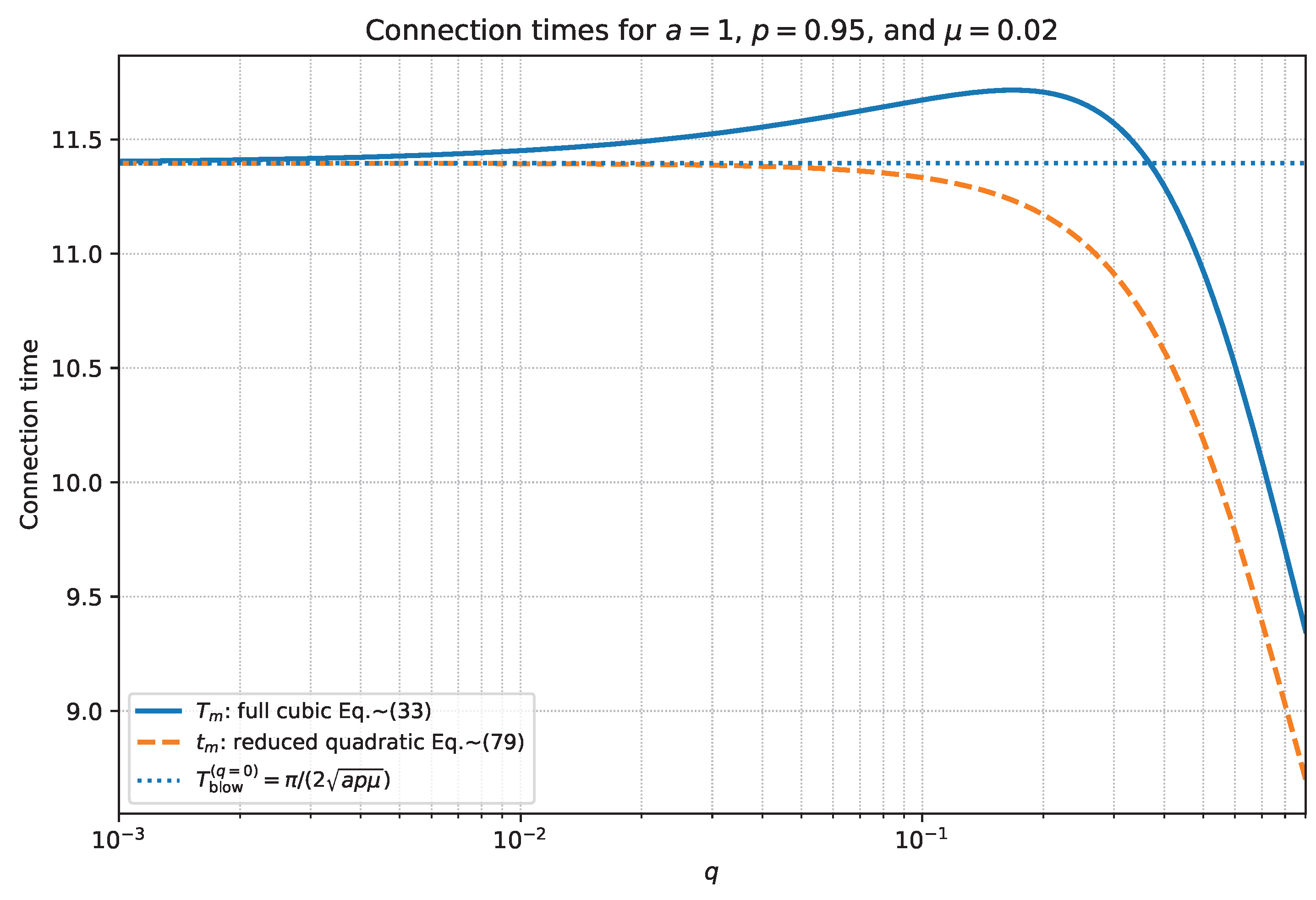
For example, when
we obtain
The connection point is
The reduced quadratic connection time in Eq. (A89) using the above is
The finite-time blow-up time of the corresponding reduced quadratic equation in Eq. (A92) is
The full cubic connection time in Eq. (A90) is obtained numerically:
For comparison, the limiting pure quadratic blow-up time obtained by setting , so that in Eq. (A93), is
These values show that, for , the full cubic trajectory reaches the very large connection point at nearly the same time that the quadratic model blows up. The reduced quadratic solution reaches slightly before its own blow-up time, whereas the full cubic solution reaches slightly after that time because the cubic term weakens the acceleration near large Z.
References
- Alligood, K., Sauer, T., & Yorke, J. [1996] Chaos: An Introduction to Dynamical Systems (Springer: New York, NY, USA).
- Ashwin, P., Wieczorek, S., Vitolo, R., & Cox, P. [2012] “Tipping points in open systems: Bifurcation, noise-induced and rate-dependent examples in the climate system,” Philosophical Transactions of the Royal Society A: Mathematical, Physical and Engineering Sciences, 370(1962), 1166–1184.
- Bender, C. M. & Orszag, S. A. [1999] Advanced Mathematical Methods for Scientists and Engineers: Asymptotic Methods and Perturbation Theory. (Springer, New York).
- Blanchard, P., Devaney, R. L., & Hall, G. R. [2012] Differential Equations, 4th ed., Cengage Learning.
- Bostrom, N. [2014]. Superintelligence. Oxford University Press.
- Callaghan, V.; Miller, J.; Yampolskiy, R.; Armstrong, S., Eds. The Technological Singularity: Managing the Journey; The Frontiers Collection; Springer: Berlin/Heidelberg, Germany, 2017. [CrossRef]
- Chalmers, D. J., 2010: The Singularity: A Philosophical Analysis. Journal of Consciousness Studies 17, no. 9–10 (2010): 9–10.
- Chen, M. A Trilemma for the Singularitarian. Philosophy & Technology 2023, 36, 62. [CrossRef]
- Dakos, V., Boulton, C., Buxton, J. et al. [2024] “Tipping point detection and early warnings in climate, ecological, and human systems,” Earth System Dynamics, 15, 1117—1135.
- Dietz, S., Rising, J., Stoerk, T., & Wagner, G. [2021] “Economic impacts of tipping points in the climate system.” Proceedings of the National Academy of Sciences, 118(34), e2103081118. [CrossRef]
- Eden, A. H. et al. (eds.), Singularity Hypotheses, The Frontiers Collection, Springer-Verlag Berlin Heidelberg 2012.
- Feudel, U. [2023] “Rate-induced tipping in ecosystems and climate: the role of unstable states, basin boundaries and transient dynamics,” Nonlin. Processes Geophys., 30, 481–502.
- Feudel, U., Pisarchik, A. N., & Showalter, K. [2018] “Multistability and tipping: From mathematics and physics to climate and brain— Minireview and preface to the focus issue.” Chaos, 28(3), 033501. [CrossRef]
- Gladwell, M. [2000] The Tipping Point: How Little Things Can Make a Big Difference. (Little Brown.).
- Grodzins, M. [1957] “Metropolitan segregation,” Scientific American 197 (October 1957), pp. 33–41.
- Good, I. J., 1965: Speculations Concerning the First Ultraintelligent Machine. Advances in Computers, Vol. 6, pp. 31–88, Academic Press, 1965.
- Hirsch, M.; Smale, S.; Devaney, R.L. Differential Equations, Dynamical Systems, and an Introduction to Chaos, 3rd ed.; Academic Press: Waltham, MA, USA, 2013; 432p.
- Holmes, M. H. [2013] Introduction to Perturbation Methods, 2nd edn., Springer, New York. [CrossRef]
- IPCC, 2021: Climate Change [2021] The Physical Science Basis. Contribution of Working Group I to the Sixth Assessment Report of the Intergovernmental Panel on Climate Change [Masson-Delmotte, V., Zhai, P., Pirani, A., Connors, S.L., Péan, C., Berger, S., Caud, N., Chen, Y., Goldfarb, L., Gomis, M.I., Huang, M., Leitzell, K., Connoy, E., Matthews, J.B.R., Maycock, T.K., Waterfield, T., Yelekçi, O., Yu, R., & Zhou, B. (eds.)]. (Cambridge University Press, Cambridge, United Kingdom and New York, NY, USA).
- Johansen, A. and Sornette, D. [2001] Finite-time singularity in the dynamics of world population, economic and financial indices, Physica A: Statistical Mechanics and its Applications, 294(3-4), 465–502.
- Kaplan, J.; McCandlish, S.; Henighan, T.; Brown, T.B.; Chess, B.; Child, R.; Gray, S.; Radford, A.; Wu, J.; Amodei, D. Scaling Laws for Neural Language Models. arXiv 2020, arXiv:2001.08361. [Google Scholar] [CrossRef].
- Kendiukhov, I. [2020] A finite-time technological singularity model with artificial intelligence self-improvement, arXiv:2010.01961 [cs.AI], https://arxiv.org/abs/2010.01961. [CrossRef]
- Kuehn, C. [2011] A mathematical framework for critical transitions: Bifurcations, fast-slow systems and stochastic dynamics. Physica D: Nonlinear Phenomena 2011, 240, 1020–1035.
- Kurzweil, R., (2006) “The Singularity is Near”, Duckworth.
- Llama Team. The Llama 3 Herd of Models. 2024. Available online: https://llama.meta.com/ (accessed on 4 July 2024).
- Lenton, T.M., Held, H., Kriegler, E., Hall, J. W., Lucht, W., Rahmstorf, S., & Schellnhuber, H. J. [2008] “Tipping elements in the Earth’s climate system,” Proceedings of the National Academy of Sciences, 105, 1786–1793.
- Lorenz, E.N. [1963] “Deterministic nonperiodic flow,” J. Atmos. Sci. 20, 130–141.
- McGuffie, K. & Henderson-Sellers, A. [2014] The Climate Modelling Primer, 4th Edition. (Wiley-Blackwell).
- Meiss, J. D. [2007] Differential Dynamical Systems. Society for Industrial and Applied Mathematics, Philadelphia. Mathematical Modeling and Computation, Vol. 14.
- Milkoreit, M., Hodbod, J., Baggio, J., Benessaiah, K., Calderón-Contreras, R., Donges, J. F., Mathias, J.-D., Rocha, J. C., Schoon, M., & Werners, S. E. [2018] “Defining tipping points for social-ecological systems scholarship — an interdisciplinary literature review.” Environmental Research Letters, 13(3), 033005. [CrossRef]
- Mucci, T., 2025: What Is the Technological Singularity? IBM Think, 2025. Available at: https://www.ibm.com/think/topics/technological-singularity (accessed 27 February 2026).
- Neishtadt, A.I. Prolongation of the loss of stability in the case of dynamic bifurcations. I. Differential Equations 1987, 23, 1385–1391. Original Russian version: Differ. Uravn. 1987, 23, 2060–2067.
- Neishtadt, A.I. Prolongation of the loss of stability in the case of dynamic bifurcations. II. Differential Equations 1988, 24, 171–176. Original Russian version: Differ. Uravn. 1988, 24, 226–233.
- Neishtadt, A. On stability loss delay for dynamical bifurcations. Discrete and Continuous Dynamical Systems - Series S 2009, 2, 897–909.
- Neishtadt, A. On maximal delay of stability loss for dynamical bifurcations. arXiv 2026, arXiv:2606.07662.
- Schelling, T. [1972] “Dynamic models of segregation.” Journal of Mathematical Sociology 1, 143–186.
- Shen, B.-W., X. Zeng, and R. Pielke Sr., 2026: Climate Tipping Revealed by Seesaws, Dominoes, and Dynamical Systems Analysis. (revised). [CrossRef]
- Shen, B.-W. [2026b] “Tipping, Nonlinear Feedback, and Bistability in a Cubic Energy Balance Model.” International Journal of Bifurcation and Chaos. Vol. 36, No. 09, 2650125. [CrossRef]
- Shen, B.-W. [2026a] “Bifurcation, tipping, and regime shifts in nonlinear energy-balance models.” International Journal of Bifurcation and Chaos. Vol. 36, No. 6, 2630014. [CrossRef]
- Shen, B.-W. [2025] “From Airy’s equation to the non-dissipative Lorenz model: turning points, quantum tunneling and solitary waves,” Encyclopedia, 5(4):208. [CrossRef]
- Shen, B.-W., Pielke Sr.,R. A., Zeng, X., Baik, J.-J., Faghih-Naini, S., Cui, J., & Atlas, R. [2021] “Is weather chaotic? Coexistence of chaos and order within a generalized Lorenz model,” Bulletin of the American Meteorological Society, 102(1), E148-E158. [CrossRef]
- Shen, B.-W. [2020]Lecture Notes on Perturbation Methods and Boundary Layer Theory; Math 537: Ordinary Differential Equations, Fall 2020; San Diego State University: San Diego, CA, USA, 2020. [CrossRef]
- Shen, B.-W. [2019] “Aggregated negative feedback in a generalized Lorenz model,” Int. J. Bifurcation and Chaos 29(3), 1950037.
- Strogatz, S. H. [2015] Nonlinear Dynamics and Chaos: With Applications to Physics, Biology, Chemistry, and Engineering, (Westview Press: Boulder, CO, USA).
- Strogatz, S. H. [2003] SYNC: The Emerging Science of Spontaneous Order. (Penguin Group).
- Thompson, J. M. T., & Sieber, J. [2011] “Predicting climate tipping as a noisy bifurcation: a review.” International Journal of Bifurcation and Chaos, 21(2), 399–423. [CrossRef]
- Thompson, N., Ge, S., & Manso, G. (2022). The importance of (exponentially more) computing power. https://arxiv.org/abs/2206.14007.
- Thorstad, D. Against the singularity hypothesis. Philosophical Studies 2025, 182, 1627–1651. [CrossRef]
- Vinge, Vernor. [1993] "The Coming Technological Singularity: How to Survive in the Post-Human Era", in Vision-21: Interdisciplinary Science and Engineering in the Era of Cyberspace, G. A. Landis, ed., NASA Publication CP-10129, pp. 11–22, 1993.
- Wikipedia contributors, “Gravitational singularity,” Wikipedia, The Free Encyclopedia, available at: https://en.wikipedia.org/wiki/Gravitational_singularity (accessed 27 February 2026).
Figure 1.
Mechanical analogy comparing cubic and quadratic ODEs. (a) Bistable W-shaped potential corresponding to the cubic ODE, with two stable equilibria (outer bowls) separated by an unstable equilibrium (central peak). (b) Degenerate W-shaped potential corresponding to the quadratic ODE, obtained by removing the right-most segment of the W-shaped landscape. This reduced geometry contains a single stable equilibrium and only one fold structure. (c) Rotated view of the degenerate potential, illustrating the single-fold (saddle-node) bifurcation. At the fold threshold, the stable and unstable equilibria merge and disappear, leaving no restoring minimum. The remaining steep segment (shown in green) acts as a cliff-like slope, along which the system rapidly accelerates once stability is lost. The dashed horizontal line marks a common reference level.
Figure 1.
Mechanical analogy comparing cubic and quadratic ODEs. (a) Bistable W-shaped potential corresponding to the cubic ODE, with two stable equilibria (outer bowls) separated by an unstable equilibrium (central peak). (b) Degenerate W-shaped potential corresponding to the quadratic ODE, obtained by removing the right-most segment of the W-shaped landscape. This reduced geometry contains a single stable equilibrium and only one fold structure. (c) Rotated view of the degenerate potential, illustrating the single-fold (saddle-node) bifurcation. At the fold threshold, the stable and unstable equilibria merge and disappear, leaving no restoring minimum. The remaining steep segment (shown in green) acts as a cliff-like slope, along which the system rapidly accelerates once stability is lost. The dashed horizontal line marks a common reference level.
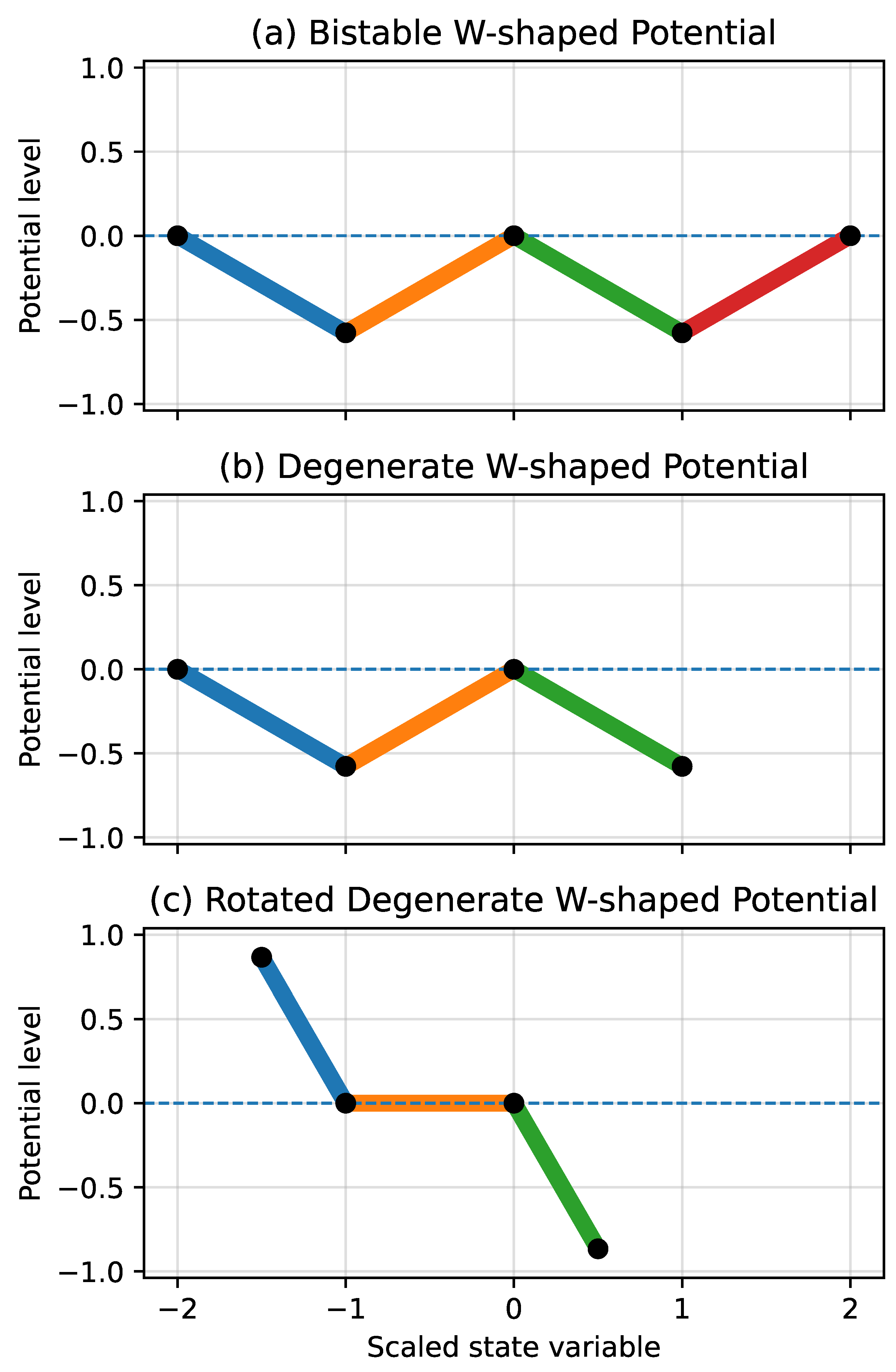
Figure 2.
Potential function and its derivatives for the unified cubic system with , , , and . (a) The potential , with critical points , , and marked in black and fold points and marked in blue. (b) The first derivative , whose zeros identify the critical points. (c) The second derivative , whose zeros identify the fold points, with the stability extremum marked in red. (d) The third derivative , whose zero identifies the stability extremum . Black, blue, and red markers denote critical points, fold points, and the stability extremum, respectively.
Figure 2.
Potential function and its derivatives for the unified cubic system with , , , and . (a) The potential , with critical points , , and marked in black and fold points and marked in blue. (b) The first derivative , whose zeros identify the critical points. (c) The second derivative , whose zeros identify the fold points, with the stability extremum marked in red. (d) The third derivative , whose zero identifies the stability extremum . Black, blue, and red markers denote critical points, fold points, and the stability extremum, respectively.
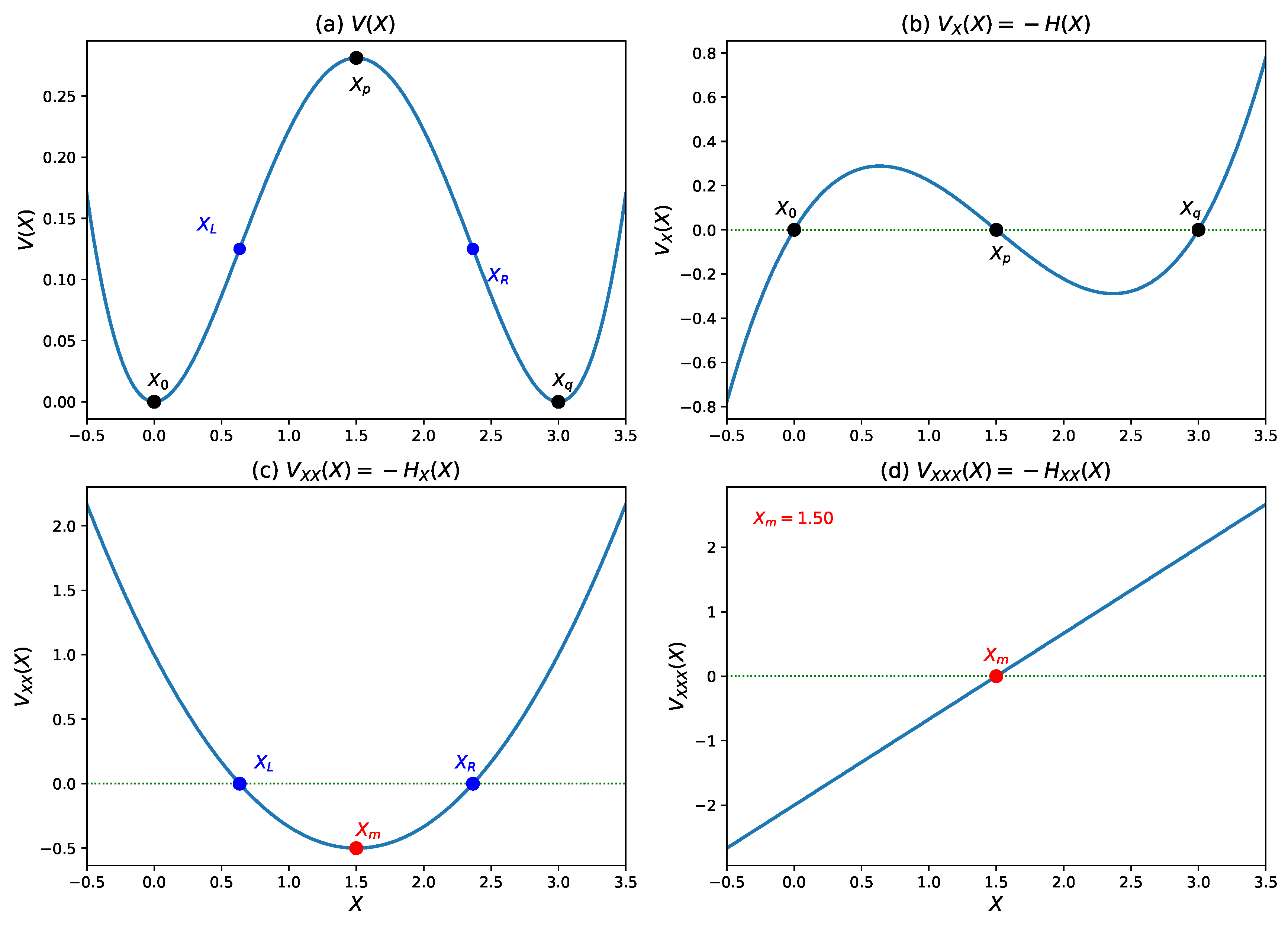
Figure 3.
Schematic comparison of the unified cubic model, the left- and right-fold-centered post-fold equations, and their reduced quadratic approximations. The left reduced equation gives a tan-type solution, which is not identical to exponential growth, while the right reduced equation gives a tanh-type solution, which is equivalent, after a suitable normalization, to a sigmoid function.
Figure 3.
Schematic comparison of the unified cubic model, the left- and right-fold-centered post-fold equations, and their reduced quadratic approximations. The left reduced equation gives a tan-type solution, which is not identical to exponential growth, while the right reduced equation gives a tanh-type solution, which is equivalent, after a suitable normalization, to a sigmoid function.
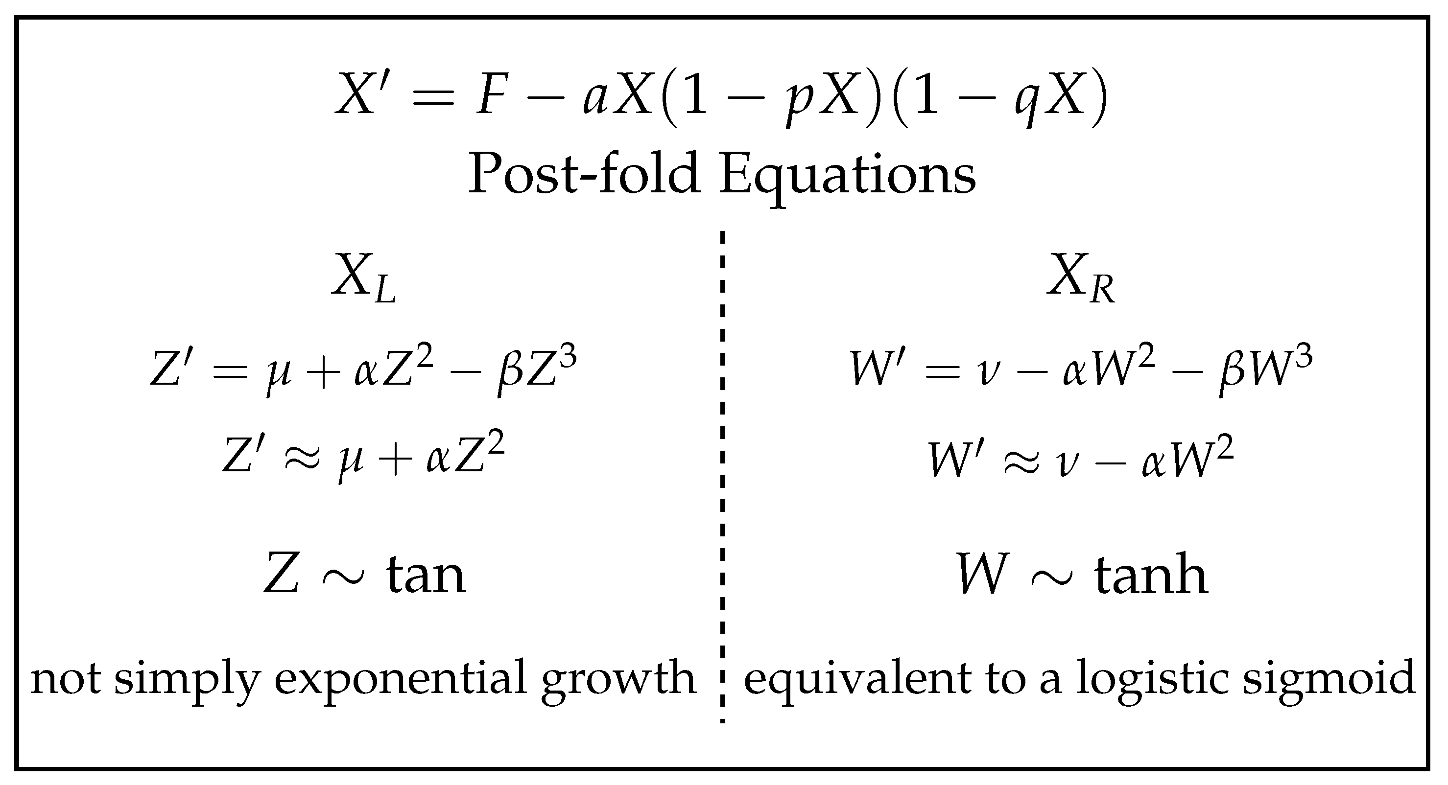
Figure 4.
Single-fold tipping dynamics for the quadratic model. The solid blue curve shows the numerical solution of the governing ODE in Eq. (19). The dashed orange curve represents the quasi-steady stable branch, and the dotted green curve denotes the quasi-steady unstable branch obtained from the corresponding algebraic equilibrium equation. The stable and unstable branches merge at the fold threshold. Beyond this point, no equilibrium exists and the trajectory undergoes a rapid, self-amplifying transition. We define the transition interval as the time span between the fold time and the diagnosed blow-up time.
Figure 4.
Single-fold tipping dynamics for the quadratic model. The solid blue curve shows the numerical solution of the governing ODE in Eq. (19). The dashed orange curve represents the quasi-steady stable branch, and the dotted green curve denotes the quasi-steady unstable branch obtained from the corresponding algebraic equilibrium equation. The stable and unstable branches merge at the fold threshold. Beyond this point, no equilibrium exists and the trajectory undergoes a rapid, self-amplifying transition. We define the transition interval as the time span between the fold time and the diagnosed blow-up time.
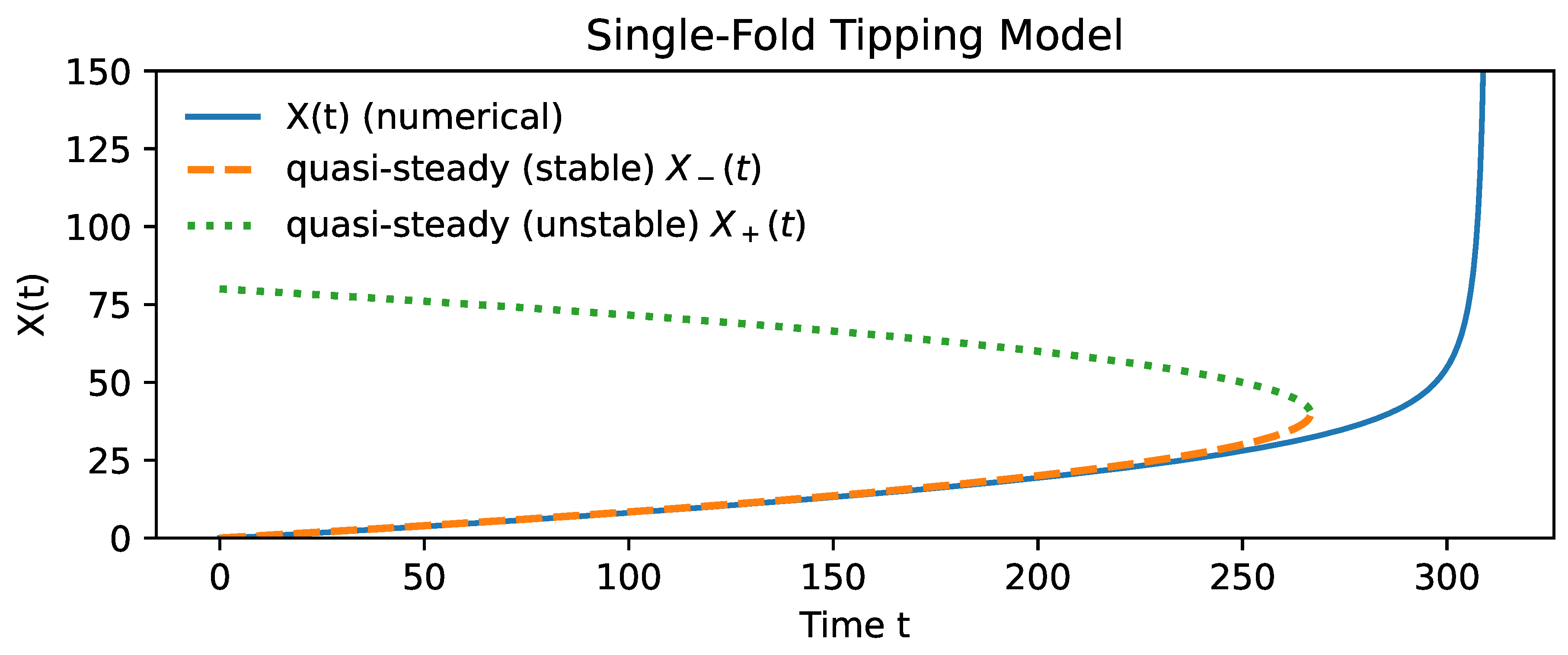
Figure 5.
Numerical solution of the full non-autonomous cubic equation compared with two fold-centered post-fold cubic approximations. The light-green curve shows the full non-autonomous cubic solution. The orange dashed curve shows the left-fold-centered post-fold approximation. The blue dashed curve with markers shows the right-fold-centered post-fold approximation, initialized at the trajectory-based time , where . The vertical dotted lines mark the left-fold time and the trajectory-based time . The horizontal dotted lines mark the fold levels and .
Figure 5.
Numerical solution of the full non-autonomous cubic equation compared with two fold-centered post-fold cubic approximations. The light-green curve shows the full non-autonomous cubic solution. The orange dashed curve shows the left-fold-centered post-fold approximation. The blue dashed curve with markers shows the right-fold-centered post-fold approximation, initialized at the trajectory-based time , where . The vertical dotted lines mark the left-fold time and the trajectory-based time . The horizontal dotted lines mark the fold levels and .
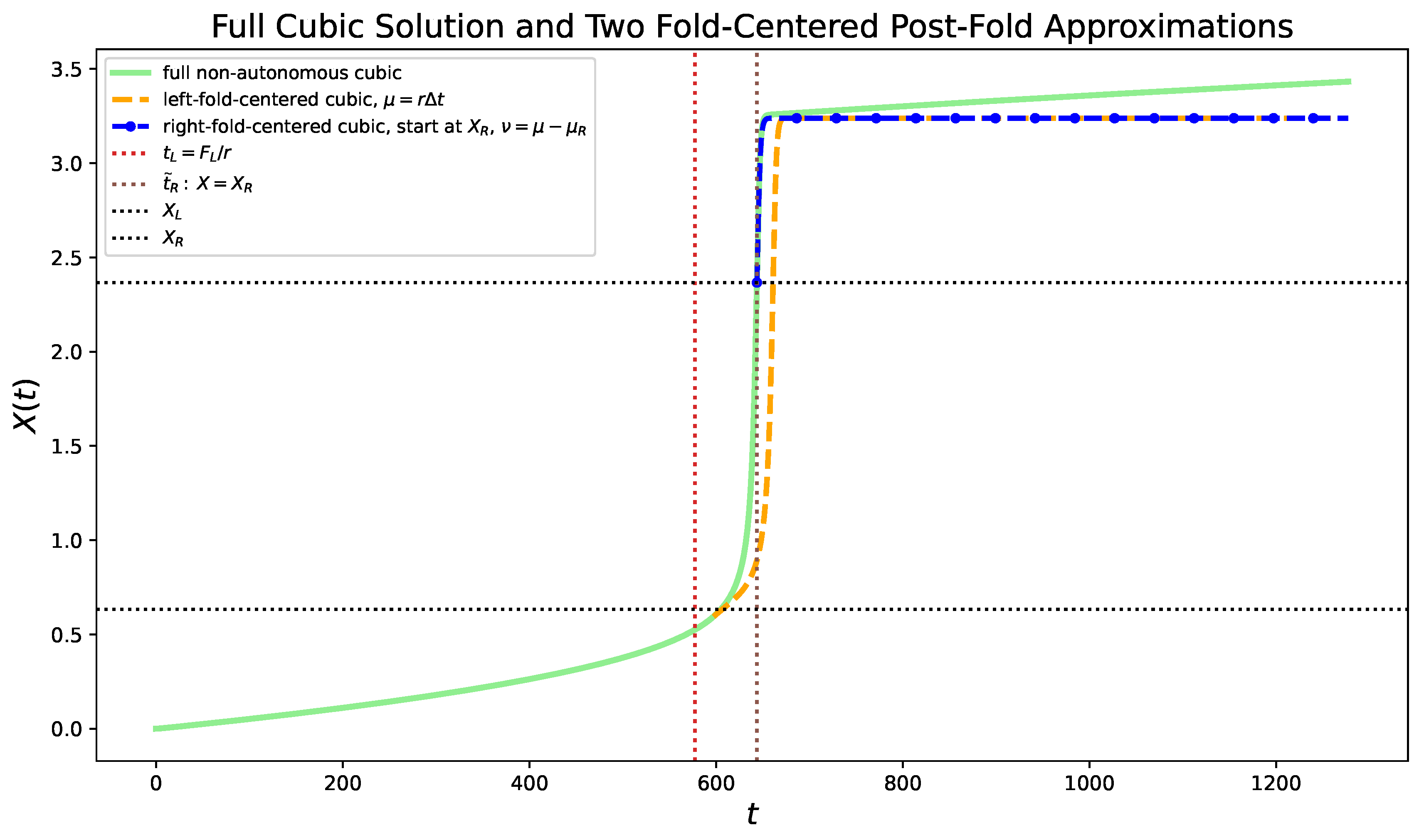
Figure 6.
-connected tan–tanh approximation and comparison with the full post-fold cubic equation. (a) The connected analytical approximation, where the tan branch describes the initial slow growth and subsequent rapid growth, while the tanh branch describes the rapid transition, slowdown, and saturation. (b) Comparison between the -connected tan–tanh approximation and the numerical solution of the full post-fold cubic equation. The horizontal dotted line marks the stability-extremum level , and the vertical dotted line marks the connection time .
Figure 6.
-connected tan–tanh approximation and comparison with the full post-fold cubic equation. (a) The connected analytical approximation, where the tan branch describes the initial slow growth and subsequent rapid growth, while the tanh branch describes the rapid transition, slowdown, and saturation. (b) Comparison between the -connected tan–tanh approximation and the numerical solution of the full post-fold cubic equation. The horizontal dotted line marks the stability-extremum level , and the vertical dotted line marks the connection time .
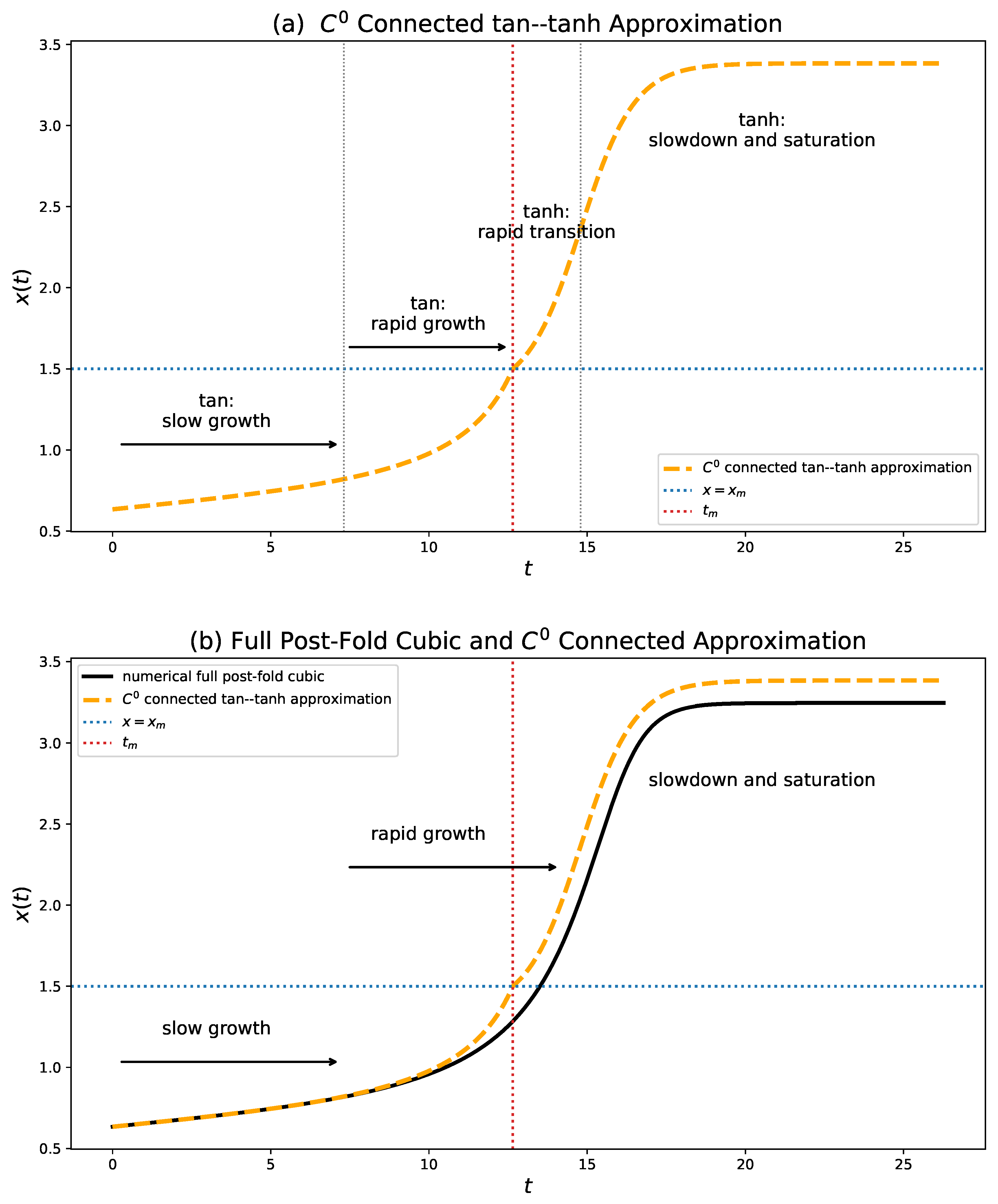

Table 1.
Hierarchy of derivative conditions for the unified cubic system. The condition identifies equilibrium points. The condition , together with , identifies fold bifurcation points. The condition , equivalently , identifies the midpoint between the two folds, where the potential curvature is most negative and the local linear growth rate is most positive.
Table 1.
Hierarchy of derivative conditions for the unified cubic system. The condition identifies equilibrium points. The condition , together with , identifies fold bifurcation points. The condition , equivalently , identifies the midpoint between the two folds, where the potential curvature is most negative and the local linear growth rate is most positive.
| Name | Condition | Location for fixed F | Alternative names & interpretation |
|---|---|---|---|
| Critical points | Equilibrium points or fixed points | ||
| Fold points | Potential inflection points or turning points | ||
| Stability maximum | Stability extremum, connection point, or potential-curvature extremum |
Table 2.
Three types of ODEs revealing finite-time singularity.
| Type | Equation | Solution | Role | Eq. No. |
| I | Airy reduction | Airy structure; delayed blow-up | (47) | |
| II | tan function | Frozen-forcing autonomous transition | (50) | |
| III | Pure quadratic self-amplification | (54) |
Table 3.
Analogy of Single-Fold Tipping and AI Singularity.
| Single-Fold Tipping | AI Singularity Analogy | |
|---|---|---|
| Stable equilibrium branch | ↔ | Constrained technological growth |
| Bifurcation (fold; loss of equilibrium) | ↔ | Threshold for recursive self-improvement |
| Transition phase | ↔ | Self-amplifying intelligence growth |
| Finite-time blow-up | ↔ | Idealized technological singularity |
Disclaimer/Publisher’s Note: The statements, opinions and data contained in all publications are solely those of the individual author(s) and contributor(s) and not of MDPI and/or the editor(s). MDPI and/or the editor(s) disclaim responsibility for any injury to people or property resulting from any ideas, methods, instructions or products referred to in the content. |
© 2026 by the authors. Licensee MDPI, Basel, Switzerland. This article is an open access article distributed under the terms and conditions of the Creative Commons Attribution (CC BY) license (http://creativecommons.org/licenses/by/4.0/).
Copyright: This open access article is published under a Creative Commons CC BY 4.0 license, which permit the free download, distribution, and reuse, provided that the author and preprint are cited in any reuse.


