

Submitted:
17 June 2026
Posted:
23 June 2026
You are already at the latest version
Abstract
Fractional Brownian motion has been widely used in financial modeling to capture long-range dependence and persistent behavior observed in asset dynamics. In the fractional Black-Scholes framework, accurate estimation of the Hurst parameter is essential, since estimation uncertainty can directly affect option pricing results. In this paper, we propose a Bayesian framework for joint inference on the Hurst parameter and volatility in fractional stochastic differential equation models. In contrast to approaches based solely on point estimation, the proposed method propagates posterior uncertainty directly into option pricing distributions under the fractional Black-Scholes model. Simulation studies are conducted across multiple values of the Hurst parameter and sample sizes to evaluate estimation accuracy, posterior coverage, and pricing uncertainty. The results demonstrate stable posterior inference and coherent uncertainty quantification for both model parameters and option prices. The methodology is further illustrated using WTI crude oil and natural gas data under different market regimes. The empirical analysis indicates that differences in market behavior are driven primarily by changes in volatility rather than strong long-range dependence, while posterior option price distributions reflect substantial variation in pricing uncertainty across regimes. These findings highlight the importance of incorporating joint parameter uncertainty in fractional financial models and demonstrate the practical value of Bayesian methods for option pricing applications.
Keywords:
fractional Brownian motion
; Hurst parameter
; Bayesian inference
; fractional Black–Scholes model
; option pricing
; long-memory processes
; posterior uncertainty
1. Introduction
The pricing of financial derivatives remains a central topic in mathematical finance, with the Black–Scholes model representing a fundamental breakthrough in the field [7,25]. By modeling asset prices through geometric Brownian motion under a no-arbitrage framework, the model provides a closed-form solution for European option pricing and has become a cornerstone of modern financial theory. Despite its widespread use, empirical studies have shown that financial time series often exhibit features that are inconsistent with the model assumptions, including long-range dependence, volatility clustering, and heavy-tailed return distributions.
Fractional Brownian motion directly addresses these shortcomings by introducing memory into the stochastic dynamics of asset prices. Fractional Brownian motion (fBm) was formally introduced by Mandelbrot Van Ness [22], who defined it as a generalization of standard Brownian motion with stationary, correlated increments. Its relevance to financial time series—particularly the presence of long-range dependence—was subsequently argued by Mandelbrot [21]. Fractional Brownian motion incorporates a Hurst parameter that characterizes long-range dependence in stochastic processes. In this framework, the Hurst parameter governs the degree of dependence in the process, while denotes the volatility. In particular, when the Hurst parameter exceeds one-half, the process exhibits persistence, reflecting the tendency of financial returns to display long memory. This has led to the development of fractional Black–Scholes models, which extend the classical framework by incorporating memory effects and providing a more flexible representation of asset dynamics [6]. More recent developments in financial modeling have also emphasized rough volatility and fractional dynamics as realistic representations of market behavior, particularly at high frequencies [3,14]. Several studies have proposed explicit formulations of such models based on fractional Brownian motion, illustrating how the Hurst parameter influences option pricing and volatility dynamics [10,16,27].
Early studies also investigated option pricing in markets driven by fractional Brownian motion and demonstrated the potential impact of long-range dependence on derivative valuation [28]. Notwithstanding these advances, the problem of jointly estimating the Hurst parameter H and the volatility within a unified statistical framework has received comparatively little attention. In particular, Bayesian approaches that simultaneously quantify uncertainty in both parameters remain underdeveloped, despite their natural suitability for this inference problem.
While fractional models offer improved realism, their practical implementation introduces significant statistical challenges. In particular, the Hurst index and volatility must be inferred from observed data, and their joint behavior directly influences pricing outcomes. Many existing approaches rely on point estimates or marginal intervals, which may fail to adequately capture the dependence between these quantities. As a result, estimation error can be misrepresented, potentially leading to inaccurate assessments in financial applications. From a practical perspective, these challenges are especially important in decision-making, where even small inaccuracies can lead to meaningful differences in option values and affect hedging strategies, risk management, and portfolio allocation.
Accurate estimation of the Hurst parameter has been a central challenge in the application of fractional models to financial data. The statistical theory of long-range dependence has been extensively developed in both Gaussian and non-Gaussian settings, with applications across telecommunications, hydrology, economics, and finance [4,12,13,33]. These developments have established the Hurst parameter as a key measure of persistence and dependence in stochastic processes.
A wide range of methods has been proposed for estimating long-range dependence, each with different trade-offs between bias, efficiency, and computational complexity. Early work by Beran [4] provided a systematic treatment of statistical methods for long-memory processes, while subsequent studies highlighted the sensitivity of classical estimators to short-range dependence and finite-sample effects [34]. Semi-parametric approaches, such as log-periodogram regression and local Whittle estimation, have been widely used because of their attractive asymptotic properties, although they often require relatively large sample sizes to achieve reliable performance [17,31]. Alternative approaches include wavelet-based estimators, which exploit the scale invariance of fractional processes and have been shown to improve estimation accuracy in certain settings [1,2]. A broader overview of commonly used Hurst exponent estimation procedures and their practical characteristics is provided by Zhang et al. [37].
Despite these developments, much of the existing literature focuses primarily on point estimation and does not fully account for uncertainty in the estimated parameters. This limitation is particularly important in financial applications, where small errors in estimating the Hurst parameter and volatility can propagate through pricing formulas and lead to substantial differences in option valuation. These considerations motivate the use of Bayesian approaches, which provide full posterior distributions and allow uncertainty in model parameters to be carried directly into subsequent inference and pricing decisions.
More recently, Bayesian approaches have been proposed as a flexible framework for estimation in long-memory models, allowing for the incorporation of prior information and providing full posterior distributions [5,8,11,20,35,36]. These methods offer a natural way to quantify uncertainty through posterior distributions. In many applications, however, inference is primarily reported through marginal posterior summaries such as posterior means and credible intervals [9,19,20].
At the same time, maximum likelihood and the method of moments estimators are known to exhibit systematic bias when applied to fractional stochastic differential equation models, particularly for values of the Hurst parameter away from 0.5. This issue has been documented in both parametric and moment-based settings [29,32], where it is shown that both maximum likelihood and method of moments estimators require bias correction for reliable practical use.
Recent work has also considered Bayesian modeling of static and dynamic Hurst parameters under stochastic volatility frameworks, further highlighting the importance of jointly modeling persistence and volatility in long-memory processes [35]. Despite these developments, the joint dependence between key parameters, such as the Hurst parameter and volatility, is often not fully captured, even though this dependence has a direct impact on derived quantities such as option prices. In particular, while bias-corrected estimators improve point estimation, they do not address the propagation of joint parameter uncertainty into financial quantities. This limitation is especially important in financial applications, where interactions between parameters can significantly influence pricing outcomes. These observations highlight the need for methods that explicitly account for joint parameter uncertainty in fractional models.
Bayesian inference provides a coherent framework for addressing these challenges by combining prior information with observed data to produce a full posterior distribution over model parameters [26]. A key advantage of the Bayesian approach is its ability to capture dependence between parameters through joint inference. In this context, joint highest-density regions (HDRs) offer a principled method for summarizing uncertainty in a multidimensional setting, providing a more accurate representation than separate marginal intervals.
Motivated by these considerations, this paper focuses on Bayesian estimation of the Hurst parameter and volatility within a fractional Gaussian noise framework. Using a simulation-based approach, we construct empirical joint highest-density regions for and evaluate their repeated-sampling performance. The results reveal strong posterior dependence between parameters and highlight the limitations of marginal interval-based inference.
To assess the practical implications of parameter uncertainty, posterior samples are propagated through the fractional Black–Scholes pricing formula to obtain distributions of option prices. This approach allows for the construction of credible intervals that reflect joint parameter uncertainty, providing a more informative basis for decision-making compared to traditional point estimates.
In this paper, we address this gap by developing a Bayesian framework for the joint estimation of H and from discretely observed asset price data following a fractional Black–Scholes model. We construct prior distributions informed by the theoretical constraints on each parameter, derive the corresponding posterior, and employ Markov chain Monte Carlo (MCMC) methods for inference. The resulting estimates are then applied to fractional option pricing, where we demonstrate that incorporating posterior uncertainty in H and leads to materially different option prices compared to approaches that treat these parameters as fixed or known. The remainder of the paper is organized as follows. Section 2 presents the fractional Black–Scholes framework and the Bayesian methodology used to jointly estimate H and , including prior specification, posterior computation, and the construction of joint highest-density regions. Section 3 reports a simulation study evaluating the performance of the proposed estimators, with emphasis on coverage, posterior dependence, and estimation accuracy. Section 4 provides an empirical application in which posterior parameter draws are propagated through the fractional Black–Scholes pricing formula to quantify option pricing uncertainty. Section 5 concludes the paper and discusses limitations and directions for future research.
2. Methodology
This section describes the simulation framework used to study Bayesian estimation of the Hurst parameter H and the scale parameter under fractional Gaussian noise (fGn). We construct joint highest-density regions (HDRs) for and assess repeated-sampling coverage with respect to the true pair .
2.1. Data-Generating Mechanism
Let denote an observed fGn sample of length n. For a fixed Hurst parameter , the lag-k autocovariance of unit-variance fGn is
Using (1), the Toeplitz correlation matrix is defined by
This Toeplitz structure is standard in long-memory Gaussian processes [4] and provides the basis for data generation in our simulation study. For fixed true values , the simulated sample is generated from the corresponding Gaussian model using this covariance structure.
where denotes the n-vector of ones.
This yields an exact Gaussian sample with mean and covariance . Cholesky factorization provides a numerically stable and computationally efficient approach for simulating Gaussian vectors with positive-definite covariance matrices [15].
2.2. Bayesian Model Specification
Conditional on , the data are modeled as
with , where in our implementation and .
The prior distributions are chosen as
where , , , and are fixed hyperparameters, following standard Bayesian modeling practice [26].
Hence, the posterior density is
where is the multivariate normal likelihood induced by (6).
2.3. Posterior Computation
Under (6), the log-likelihood is
which follows from the multivariate Gaussian likelihood [4]. To compute this efficiently, we use the Cholesky factorization
so that
and the quadratic form is evaluated through triangular solves rather than direct matrix inversion, which improves numerical stability and computational efficiency.
2.4. Bayesian Implementation
To facilitate efficient MCMC sampling and avoid boundary issues, we work with transformed parameters [9]. For the volatility parameter , we define . For the Hurst parameter , we apply a logit transformation
which maps H to the real line. The corresponding Jacobian adjustments are included in the posterior target density.
Posterior inference is carried out using a Metropolis-within-Gibbs scheme with random-walk proposals [9]. To improve sampling efficiency, we incorporate a joint block update for , motivated by their strong posterior dependence. The proposal covariance is estimated from a preliminary pilot run and used to construct a bivariate Gaussian random-walk proposal aligned with the posterior geometry. This substantially improves mixing in regions of high posterior curvature.
2.5. Joint Highest-Density Region Coverage
Following the posterior sampling step, we evaluate the transformed posterior log-density at each draw as
which is used to construct the joint highest-density regions.
The transformed posterior log-density is evaluated at each retained posterior draw , producing a set of posterior heights . These values are ranked from largest to smallest. For a target probability level , we retain the top posterior draws following the highest-density region (HDR) construction of [18]. The retained subset defines an empirical joint HDR for :
where is the empirical cutoff corresponding to the top fraction of posterior heights. This construction is preferable to separate marginal intervals for H and , since the posterior draws exhibit substantial dependence and lie on a curved ridge rather than in an approximately rectangular region.
To evaluate repeated-sampling performance, we repeat the above procedure over B simulated datasets. For each replication, we check whether the true parameter pair lies inside the estimated joint HDR:
The empirical coverage is then
In addition, we summarize posterior medians, biases and posterior correlations between H and .
2.6. Posterior Option Pricing
To connect parameter uncertainty with option pricing, each retained posterior draw is mapped through the fractional Black–Scholes pricing framework [6,16,27]. The pricing equation is used here as a sensitivity-based mechanism for propagating posterior uncertainty in into option values. Let
Then
and the call price is
where denotes the standard normal distribution function.
Applying (23) to every posterior draw produces a posterior sample of option prices,
from which posterior medians and credible intervals for the option price are obtained.
3. Simulation Study
This section evaluates the repeated-sampling performance of the proposed Bayesian procedure under fractional Gaussian noise. For each replication, we (i) generate an exact Gaussian fGn sample from the true covariance structure, (ii) estimate via Bayesian MCMC under the multivariate normal model, (iii) construct an empirical joint HDR by ranking posterior draws according to posterior height, (iv) record whether the true pair falls inside the estimated HDR, and (v) propagate posterior draws through the fractional Black–Scholes formula to obtain a posterior distribution for the call price.
Posterior inference was based on 3,000 MCMC iterations following an initial pilot run of 1,000 iterations. The first 500 iterations of the main chain were discarded as burn-in, leaving 2,500 posterior draws for inference. For each design point, 100 simulated datasets were generated. Computation times are based on a MacBook Air with an Apple M4 processor and 24GB of RAM. Approximate runtimes for the full simulation grid under the sequential implementation were 6.6 minutes for , 16.9 minutes for , and 4.5 hours for , demonstrating the substantial increase in computational cost as sample size grows. The largest setting, , required approximately 72 hours under the sequential implementation. To improve computational efficiency, a parallelized version of the simulation procedure was also implemented, reducing the runtime for to approximately four hours while producing qualitatively consistent results.
Across all simulation settings, estimation accuracy improved as the sample size increased, with narrower posterior regions and reduced bias observed for larger values of n. However, the overall pricing behavior and uncertainty structure remained qualitatively similar for . This suggests that moderate sample sizes already provide stable inference for the proposed Bayesian framework while avoiding the substantially higher computational cost associated with larger datasets. Similar computational trade-offs have been noted in recent studies of Bayesian Hurst exponent estimation for long-memory models [24].
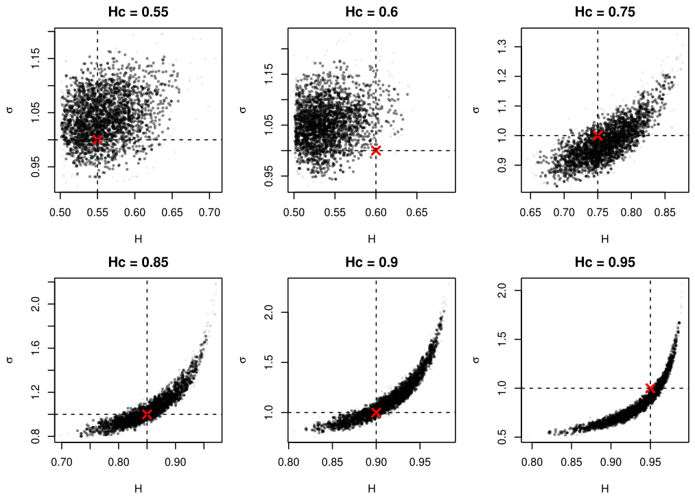
Figure 1 and Figure 2 illustrate the joint posterior draws and corresponding 95% HDR clouds for the smallest and largest sample sizes considered. These figures demonstrate the substantial posterior dependence between H and and show the improvement in posterior concentration as sample size increases. Corresponding results for the intermediate sample sizes and are provided in Appendix A. Figure 3a–d summarize empirical coverage and posterior dependence across sample sizes on a common scale. Coverage remains close to the nominal 0.95 level across most settings, while generally increases with , indicating that separate marginal intervals may fail to capture important joint posterior structure.
It is well known that fractional Brownian motion models may violate the semimartingale structure underlying classical arbitrage-free pricing theory [6,30]. Consequently, the fractional Black–Scholes framework is used here primarily as a sensitivity-based tool for studying how posterior uncertainty in propagates into option values, rather than as a complete market equilibrium model under all fractional specifications. Nevertheless, recent developments in rough volatility modeling further supports the usefulness of fractional dynamics as flexible representations of financial dependence structures [3,14].
To quantify the implications for option valuation, Figure 4 reports posterior medians and 95% credible intervals for the call price obtained by mapping posterior draws through the fractional Black–Scholes pricing equation. The results show a clear decline in the posterior median call price as increases, with the decrease becoming especially pronounced when approaches one. This behavior indicates that, under the chosen option-pricing parameters, stronger persistence can substantially reduce the recommended posterior median call price.
The uncertainty bands also widen noticeably for larger values of , particularly near and . In this region, the posterior price distributions become more dispersed and appear left-skewed, with lower posterior medians observed for smaller sample sizes. This suggests that when the true dependence is very strong, limited sample sizes may lead to greater uncertainty and more conservative pricing recommendations.
From a practical perspective, increasing the sample size improves posterior concentration, but the gain must be balanced against computational cost. The difference between and is relatively small compared with the substantial increase in runtime required for . In contrast, produces wider intervals, but these intervals often contain the corresponding intervals for larger sample sizes. Therefore, may be sufficient for exploratory analysis or preliminary pricing decisions, while provides a more reliable compromise between statistical precision and computational feasibility. The use of is recommended only when very high precision is required or when parallel computation is available. Table 1 provides the corresponding numerical summaries, including the 95% interval and the 90% band , which may be interpreted as a conservative bid–ask range.
Figure 5 displays the posterior lower, median, and upper quantile curves of the option price as functions of the true Hurst parameter for each sample size. The lower and upper curves form a 95% credible interval. The shrinkage of the gap between and as n increases illustrates posterior concentration in the joint parameter space. The median call price decreases with under the chosen option parameters, while uncertainty is substantially larger for small samples and tightens as n increases. These quantile curves also facilitate decision-oriented summaries, such as one-sided credible bounds, which may be preferable when overpricing and underpricing have asymmetric consequences.
4. Empirical Application
This section illustrates the practical performance of the proposed Bayesian framework using real financial data from energy markets. We consider daily log returns of WTI crude oil and natural gas futures, which are known for their pronounced volatility and relevance in derivative pricing applications.
To investigate the effect of market conditions, the oil data are divided into two distinct periods representing different volatility regimes. The first period corresponds to a high-volatility environment, while the second reflects relatively stable market behavior. Natural gas is included as an additional example of a persistently volatile asset, allowing us to examine the robustness of the proposed approach across different settings.
For each dataset, we estimate the Hurst parameter and volatility using the Bayesian methodology described in the previous section. These estimates are then incorporated into the fractional Black–Scholes framework to obtain posterior distributions of option prices. This approach allows us to assess not only point estimates but also the uncertainty associated with pricing decisions.
The empirical analysis is designed to distinguish between volatility-driven effects and genuine long-range dependence, and to quantify their impact on option pricing. This distinction is particularly important, as traditional methods may confound volatility with persistence, leading to misleading inference.
4.1. WTI Crude Oil: Regime Comparison
We begin with WTI crude oil, which exhibits distinct regimes of market behavior. The period 2020–2022 is characterized by elevated volatility, while 2023–2025 reflects comparatively more stable market conditions. This provides a natural setting for examining how changes in market volatility influence posterior inference and option pricing uncertainty.
Table 2 shows that the earlier period exhibits substantially higher volatility, while the average returns remain close to zero in both regimes. This suggests that differences between the two periods are driven primarily by changes in market variability rather than systematic shifts in mean returns.
For pricing, we consider a European call option with , , , and , holding these contract inputs fixed when comparing classical Black–Scholes and fractional Black–Scholes prices.
Table 3 reports posterior summaries for the Hurst parameter and volatility. Across both periods, the estimated Hurst parameter remains close to 0.5, indicating weak long-range dependence in returns. In contrast, posterior volatility estimates differ substantially between periods, with the 2020–2022 regime exhibiting considerably higher uncertainty. The wider posterior pricing interval during this period, with a width 1.63 compared to 0.59 in the later regime, indicates that elevated volatility translates directly into greater uncertainty in option valuation.
Figure 6 further illustrates that the posterior distribution of the Hurst parameter remains relatively stable across periods, whereas volatility exhibits substantial variation between market regimes. The posterior clouds also reveal noticeable dependence between H and , emphasizing the importance of joint uncertainty quantification in the Bayesian framework.
The fractional Black–Scholes formula is used here as a sensitivity-based pricing framework to study how posterior uncertainty in propagates into option values, rather than as a claim of complete market arbitrage-free dynamics under all fractional specifications.
Figure 7 shows that the high-volatility period produces a substantially wider posterior distribution of option prices, reflecting increased pricing uncertainty. In contrast, the more stable 2023–2025 regime yields a considerably tighter distribution. Although the posterior median prices remain reasonably close to the corresponding classical Black–Scholes prices, the range of plausible option values differs substantially across market regimes.
Overall, these findings suggest that differences in market regimes affect option pricing uncertainty primarily through changes in volatility rather than through strong long-range dependence in returns.
4.2. Natural Gas: High-Volatility Market
We next consider natural gas as an example of a persistently high-volatility commodity market. In contrast to the regime-based behavior observed in oil, natural gas exhibits consistently high volatility over the entire sample period.

Table 4.
Summary statistics for the natural gas return series used in the empirical analysis.
| Asset | Ticker | Period | n | Mean Return | Annualized Volatility |
|---|---|---|---|---|---|
| Natural Gas Futures | NG=F | 2022–2024 | 711 | 0.832 |
For pricing, we consider a European call with , , , and , holding these contract inputs fixed when comparing BSM and fBSM prices.
Table 5 reports posterior summaries of the Hurst parameter and volatility. The estimated Hurst parameter remains close to 0.5, indicating weak long-range dependence in returns. In contrast, the volatility is relatively high, reflecting the pronounced variability of the natural gas market. The corresponding posterior pricing interval width of 1.62 further indicates substantial uncertainty in option valuation under highly volatile market conditions.
The joint posterior distribution in Figure 8 reveals a concentration of H around 0.5, while the volatility parameter displays considerable variability. This pattern suggests that the observed dynamics are primarily driven by volatility rather than persistence. The substantial posterior dispersion in also contributes directly to the wider range of plausible option prices observed under the fractional pricing framework.
Figure 9 illustrates the posterior distribution of option prices. The posterior distribution is relatively wide, reflecting substantial uncertainty in pricing outcomes. Although the classical Black–Scholes price lies within the posterior pricing interval, it represents only a single point estimate and therefore does not capture the full uncertainty associated with the joint estimation of .
Overall, these results indicate that, in highly volatile markets, parameter uncertainty can translate into meaningful variation in option values, even in the absence of strong long-range dependence.
5. Discussion and Conclusions
This paper develops a Bayesian framework for estimating the Hurst parameter and volatility in the fractional Black–Scholes model and examines their impact on option pricing in energy markets. The empirical results provide several important insights.
First, across all datasets considered, the estimated Hurst parameter remains close to 0.5, suggesting weak evidence of long-range dependence in returns despite elevated market volatility. This finding is consistent across different assets and market conditions, indicating that persistence plays a limited role in describing return dynamics. Although the estimated Hurst parameter for returns remains close to 0.5, financial markets may still exhibit persistence in volatility dynamics, which is consistent with the broader literature on volatility clustering and rough volatility models. This suggests that fractional dynamics may remain useful for uncertainty quantification even when strong long-range dependence is not directly observed in return series.
However, the posterior distributions also demonstrate non-negligible uncertainty surrounding these estimates. Consequently, the analysis does not support imposing the classical Brownian motion assumption with certainty. From a risk management perspective, it is preferable to allow for the possibility that the true persistence structure may deviate from standard Brownian motion, even if the posterior center lies near 0.5. The Bayesian framework, therefore, provides a natural mechanism for incorporating parameter uncertainty directly into inference and option pricing, thereby avoiding overconfidence in a single fixed persistence assumption. In this sense, the fractional model serves not only as a tool for detecting strong long-range dependence, but also as a framework for quantifying uncertainty about persistence in financial markets.
An important contribution of the proposed framework is not necessarily the detection of strong long-range dependence itself, but rather the quantification of uncertainty surrounding persistence. Although the posterior distributions of the Hurst parameter were centered near 0.5 in the empirical applications, the results do not support treating the classical Brownian motion assumption H = 0.5 as known with certainty. Instead, the Bayesian framework provides a probabilistic assessment of persistence by propagating uncertainty in the Hurst parameter directly into option pricing inference. Consequently, the methodology remains informative even when strong long-range dependence is not conclusively supported by the data, since uncertainty regarding persistence can still influence financial decision-making and risk assessment.
Second, volatility emerges as the primary driver of market behavior. In the case of WTI crude oil, the comparison of two distinct periods reveals that differences in market regimes are characterized by substantial changes in volatility, while the Hurst parameter remains relatively stable. Similarly, natural gas exhibits consistently high volatility, leading to greater uncertainty in parameter estimates.
Third, these differences in volatility translate directly into differences in option pricing uncertainty. While the median fractional Black–Scholes prices remain close to the classical Black–Scholes values, the posterior distributions reveal that the range of possible option prices can vary considerably, particularly in high-volatility environments. This highlights that classical pricing models may underestimate the uncertainty associated with option valuation.
From a methodological perspective, the results emphasize the importance of jointly modeling dependence and volatility. The Bayesian approach provides a flexible framework that captures parameter uncertainty and avoids over-reliance on point estimates. These findings are consistent with recent studies emphasizing the advantages of Bayesian approaches for uncertainty quantification in long-memory estimation problems [23,24]. In contrast, methods based solely on moment conditions may be more sensitive to volatility-driven variation, potentially leading to misleading interpretations of persistence.
Overall, the findings suggest that, in financial markets, uncertainty in volatility plays a more significant role than long-range dependence in determining option prices. This has important implications for risk management, as it indicates that accounting for parameter uncertainty is essential for accurate pricing and hedging decisions.
This study has several limitations. The return series are modeled using a Gaussian fractional Gaussian noise likelihood with a constant volatility parameter within each sample period. Consequently, the framework does not explicitly account for stochastic volatility, jumps, heavy tails, or structural breaks that may arise in financial markets. In addition, the empirical analysis is based on daily data, which may mask microstructure effects and intraday dependence patterns.
Future research may extend this framework to incorporate stochastic volatility models, alternative prior structures, and heavy-tailed likelihoods. Additional directions include applications to high-frequency financial data and the integration of fractional dynamics with more complex market mechanisms such as jumps, leverage effects, and regime-switching behavior. Overall, the proposed Bayesian framework demonstrates that uncertainty quantification in fractional financial models can provide valuable insight into the stability and reliability of option pricing decisions under complex market conditions.
Author Contributions
Conceptualization, E.B. and R.G.; methodology, H.S.; software, H.S.; validation, E.B. and R.G.; formal analysis, H.S.; investigation, H.S.; resources, R.G.; data curation, H.S.; writing—original draft preparation, H.S.; writing—review and editing, E.B and R.G.; visualization, H.S.; supervision, E.B.; project administration, R.G.
Institutional Review Board Statement
Not applicable. No humans were involved in the study.
Informed Consent Statement
Not applicable. No humans were used in this study.
Data Availability Statement
The data used in the empirical application are publicly available financial market data obtained from Yahoo Finance. Simulated datasets used in the simulation study were generated using the methodology described in the paper. The R code and data supporting the findings of this study are available from the corresponding author upon reasonable request.
Acknowledgments
Hana Sagor would like to thank supervisors Ryad A. Ghanam and Edward L. Boone for their guidance, encouragement, and continuous support throughout this research. I also gratefully acknowledge the University of Jeddah, Saudi Arabia, for their support during my PhD studies. Additional thanks are extended to the Department of Statistical Sciences and Operations Research at Virginia Commonwealth University. Ryad A. Ghanam and Edward L. Boone would like to thank VCUQatar and Qatar Foundation for their funding through the Mathematical Data Science Lab.
Conflicts of Interest
The authors declare no conflict of interest.
Appendix A. Additional Posterior Diagnostic Figures
Figure A1.
Joint posterior draws and 95% HDR cloud for (gray: posterior draws; darker: top 95% HDR; red marker: true ).
Figure A1.
Joint posterior draws and 95% HDR cloud for (gray: posterior draws; darker: top 95% HDR; red marker: true ).
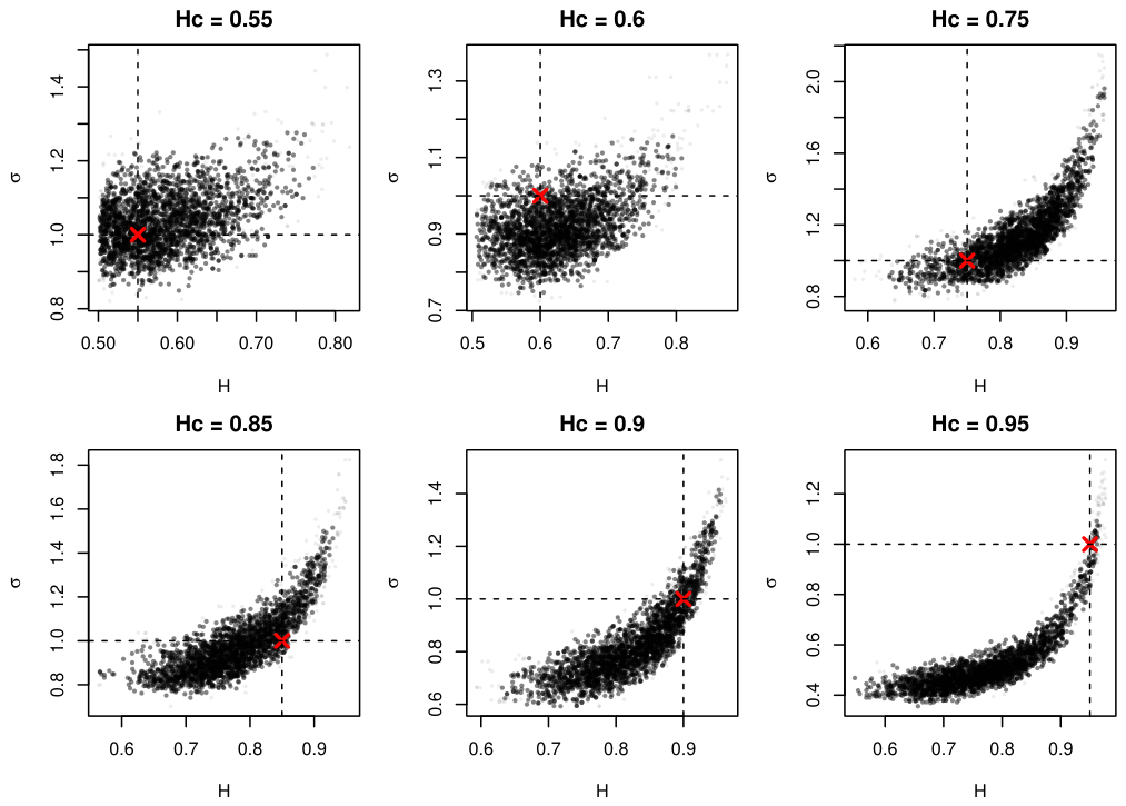
Figure A2.
Joint posterior draws and 95% HDR cloud for (gray: posterior draws; darker: top 95% HDR; red marker: true ).
Figure A2.
Joint posterior draws and 95% HDR cloud for (gray: posterior draws; darker: top 95% HDR; red marker: true ).
References
- Abry, P.; Veitch, D. Wavelet analysis of long-range dependent traffic. IEEE Trans. Inf. Theory 1998, 44(1), 2–15. [Google Scholar] [CrossRef]
- Bardet, J. M.; Lang, G.; Moulines, E.; Soulier, P. Wavelet estimator of long-range dependent processes. Stat. Inference Stoch. Process. 2000, 3(1), 85–99. [Google Scholar] [CrossRef]
- Bennedsen, M.; Lunde, A.; Pakkanen, M. S. Decoupling the short- and long-term behavior of stochastic volatility. J. Financ. Econom. 2022, 20(5), 961–1006. [Google Scholar] [CrossRef]
- Beran, J. Statistics for Long-Memory Processes; Chapman & Hall, New York, 1994. [Google Scholar]
- Beskos, A.; Dureau, J.; Kalogeropoulos, K. Bayesian inference for partially observed stochastic differential equations driven by fractional Brownian motion. Biometrika 2015, 102(4), 809–827. [Google Scholar] [CrossRef]
- Biagini, F.; Hu, Y.; ksendal, B.; Zhang, T. Stochastic calculus for fractional Brownian motion and applications; Springer, 2008. [Google Scholar] [CrossRef]
- Black, F.; Scholes, M. The pricing of options and corporate liabilities. J. Political Econ. 1973, 81(3), 637–654. [Google Scholar] [CrossRef] [PubMed]
- Chen, C.-Y.; Shafie, K.; Lin, Y.-K. Bayesian estimation of the Hurst parameter of fractional Brownian motion. Commun. Stat. – Simul. Comput. 2017, 46(6), 4760–4766. [Google Scholar] [CrossRef]
- Chopin, N.; Papaspiliopoulos, O. An Introduction to Sequential Monte Carlo; Springer, 2020. [Google Scholar] [CrossRef]
- Comte, F.; Renault, E. Long memory in continuous-time stochastic volatility models. Math. Financ. 1998, 8(4), 291–323. [Google Scholar] [CrossRef]
- Dlask, M.; Kukal, J.; Vyšata, O. Bayesian approach to Hurst exponent estimation. Methodol. Comput. Appl. Probab. 2017, 19(3), 973–983. [Google Scholar] [CrossRef]
- Doukhan, P.; Oppenheim, G.; Taqqu, M. S. (Eds.) Theory and Applications of Long-Range Dependence; Birkhäuser: Boston, MA, 2003. [Google Scholar]
- Embrechts, P.; Maejima, M. Selfsimilar Processes; Princeton University Press: Princeton, NJ, 2002. [Google Scholar]
- Gatheral, J.; Jaisson, T.; Rosenbaum, M. Volatility is rough. Quant. Financ. 2018, 18(6), 933–949. [Google Scholar] [CrossRef]
- Golub, G. H.; Van Loan, C. F. Matrix Computations, 4th ed.; Johns Hopkins University Press: Baltimore, MD, 2013. [Google Scholar]
- Hu, Y.; ksendal, B. Fractional white noise calculus and applications to finance. Infin. Dimens. Anal. Quantum Probab. Relat. Top. 2003, 6(1), 1–32. [Google Scholar] [CrossRef]
- Hurvich, C. M.; Deo, R.; Brodsky, J. The mean squared error of Geweke and Porter-Hudak’s estimator. J. Time Ser. Anal. 1998, 19(1), 19–46. [Google Scholar] [CrossRef]
- Hyndman, R. J. Computing and graphing highest density regions. Am. Stat. 1996, 50(2), 120–126. [Google Scholar] [CrossRef]
- Jacquier, E.; Polson, N. G.; Rossi, P. E. Bayesian analysis of stochastic volatility models. J. Bus. Econ. Stat. 1994, 12(4), 371–389. [Google Scholar] [CrossRef]
- Makarava, N.; Holschneider, M. Estimation of the Hurst exponent from noisy data: A Bayesian approach. Eur. Phys. J. B 2012, 85, 379. [Google Scholar] [CrossRef]
- Mandelbrot, B. B. When can price be arbitraged efficiently? A limit to the validity of the random walk and martingale models. Rev. Econ. Stat. 1971, 53(3), 225–236. Available online: https://www.jstor.org/stable/1937966. [CrossRef]
- Mandelbrot, B.; Van Ness, J. Fractional Brownian motions, fractional noises and applications. SIAM Rev. 1968, 10(4), 422–437. [Google Scholar] [CrossRef]
- Mangalam, M.; Likens, A. D. Precision in Brief: The Bayesian Hurst–Kolmogorov Method for the Assessment of Long-Range Temporal Correlations in Short Behavioral Time Series. Entropy 2025, 27(5), 500. [Google Scholar] [CrossRef] [PubMed]
- Mangalam, M.; Wilson, T. J.; Sommerfeld, J. H.; Likens, A. D. Optimizing a Bayesian method for estimating the Hurst exponent in behavioral sciences. Axioms 2025, 14(6), 421. [Google Scholar] [CrossRef]
- Merton, R. C. Theory of rational option pricing. Bell J. Econ. 1973, 4(1), 141–183. [Google Scholar] [CrossRef]
- Murphy, K. P. Machine learning: A probabilistic perspective; MIT Press, 2012; Available online: https://mitpress.mit.edu/9780262018029.
- Njomen Njomen, D. A.; Djeutcha, E. Solving Black–Scholes equation using standard fractional Brownian motion. J. Math. Res. 2019, 11(2), 142–149. [Google Scholar] [CrossRef]
- Necula, C. Option Pricing in a Fractional Brownian Motion Environment. SSRN Electron. J. 2002. [Google Scholar] [CrossRef]
- Pramanik, P.; Boone, E. L.; Ghanam, R. A. Parametric estimation in fractional stochastic differential equation. Stats 2024, 7(3), 745–760. [Google Scholar] [CrossRef]
- Rogers, L. C. G. Arbitrage with fractional Brownian motion. Math. Financ. 1997, 7(1), 95–105. [Google Scholar] [CrossRef]
- Robinson, P. M. Gaussian semiparametric estimation of long range dependence. Ann. Stat. 1995, 23(5), 1630–1661. [Google Scholar] [CrossRef]
- Sagor, H.; Boone, E. L.; Ghanam, R. A. Bias-corrected method of moments estimation of the Hurst parameter for improved option pricing under the fractional Black–Scholes model. J. Risk Financ. Manag. 2025, 18(10), 588. [Google Scholar] [CrossRef]
- Samorodnitsky, G.; Taqqu, M. S. Stable Non-Gaussian Random Processes: Stochastic Models with Infinite Variance; Chapman & Hall: New York, NY, 1994. [Google Scholar] [CrossRef]
- Taqqu, M. S.; Teverovsky, V.; Willinger, W. Estimators for long-range dependence: An empirical study. Fractals 1995, 3(4), 785–798. [Google Scholar] [CrossRef]
- Tsionas, M. G. Bayesian analysis of static and dynamic Hurst parameters under stochastic volatility. Phys. A Stat. Mech. Its Appl. 2021, 567, 125647. [Google Scholar] [CrossRef]
- Weron, R. Estimating long-range dependence: Finite sample properties and confidence intervals. Phys. A Stat. Mech. Its Appl. 2002, 312(1–2), 285–299. [Google Scholar] [CrossRef]
- Zhang, H.-Y.; Feng, Z.-Q.; Feng, S.-Y.; Zhou, Y. Typical algorithms for estimating Hurst exponent of time sequence: A comprehensive review with pseudo-code implementations. IEEE Access 2024, 12, 185528–185556. [Google Scholar] [CrossRef]
Figure 1.
Joint posterior draws and 95% HDR cloud for (gray: posterior draws; darker: top 95% HDR; red marker: true ).
Figure 1.
Joint posterior draws and 95% HDR cloud for (gray: posterior draws; darker: top 95% HDR; red marker: true ).
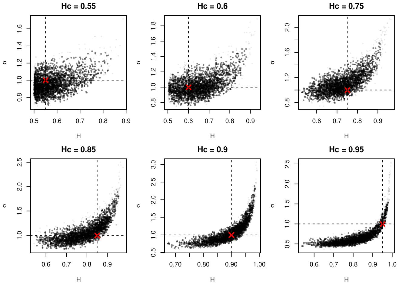
Figure 2.
Joint posterior draws and 95% HDR cloud for (gray: posterior draws; darker: top 95% HDR; red marker: true ).
Figure 2.
Joint posterior draws and 95% HDR cloud for (gray: posterior draws; darker: top 95% HDR; red marker: true ).
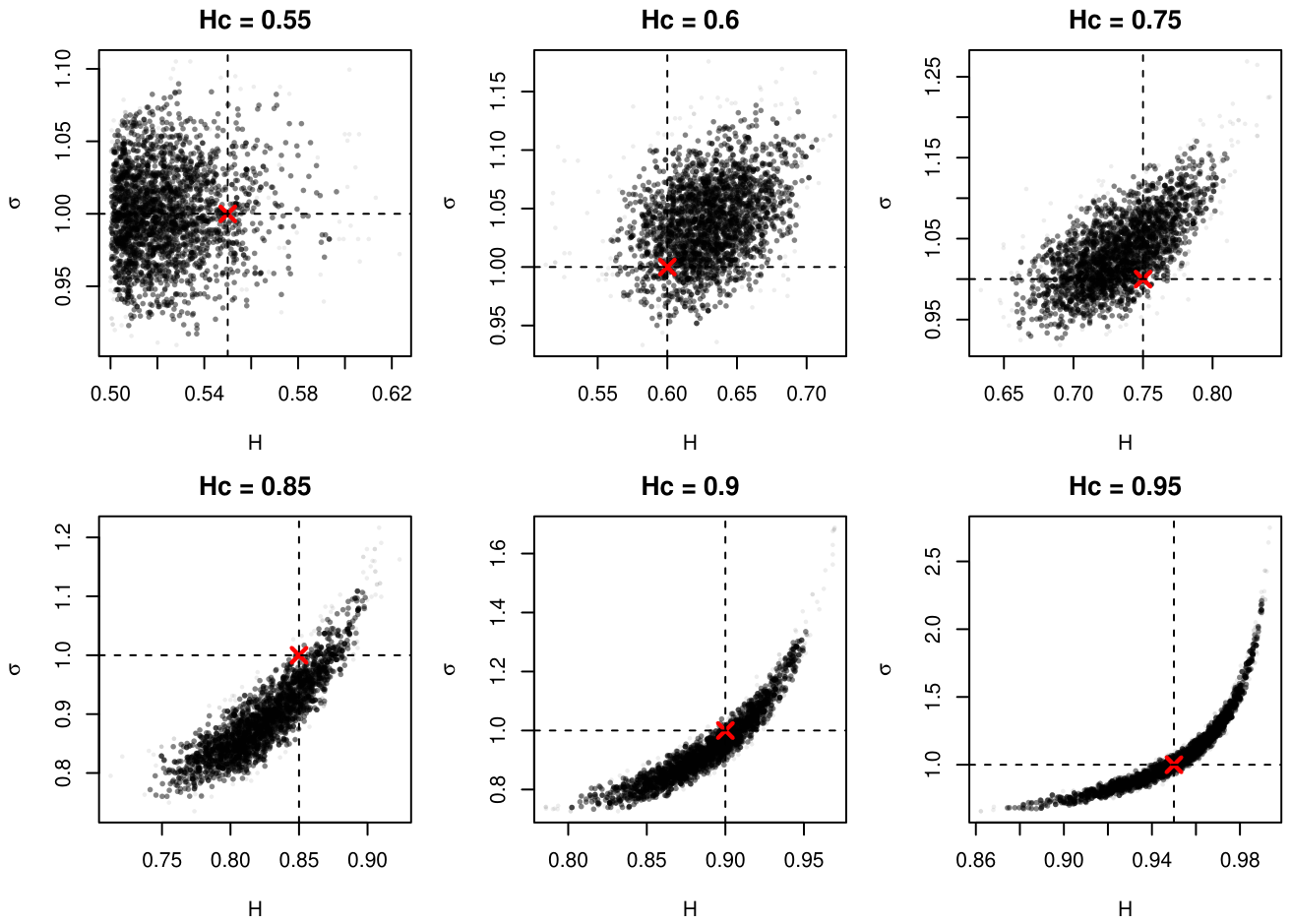
Figure 3.
Summary panels for the simulation study. Each line corresponds to a different sample size .
Figure 3.
Summary panels for the simulation study. Each line corresponds to a different sample size .
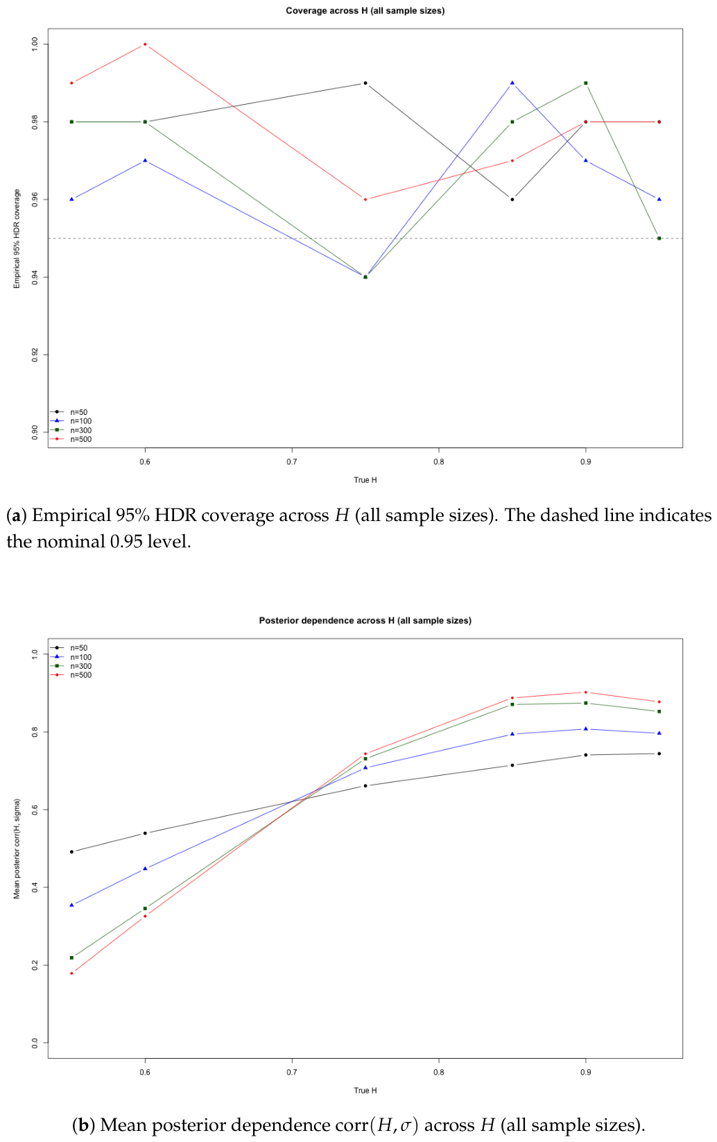
Figure 4.
Recommended call price (posterior median) versus the true Hurst parameter with 95% posterior intervals. Curves correspond to sample sizes .
Figure 4.
Recommended call price (posterior median) versus the true Hurst parameter with 95% posterior intervals. Curves correspond to sample sizes .
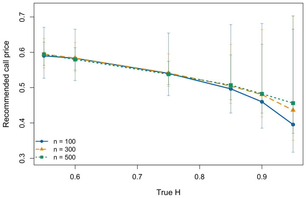
Figure 5.
Posterior call-price quantiles as functions of the true Hurst parameter . Each panel corresponds to a different sample size . Solid lines represent the posterior median , while dashed lines represent the lower and upper 95% credible bounds and . Interval width decreases as n increases, reflecting posterior concentration.
Figure 5.
Posterior call-price quantiles as functions of the true Hurst parameter . Each panel corresponds to a different sample size . Solid lines represent the posterior median , while dashed lines represent the lower and upper 95% credible bounds and . Interval width decreases as n increases, reflecting posterior concentration.
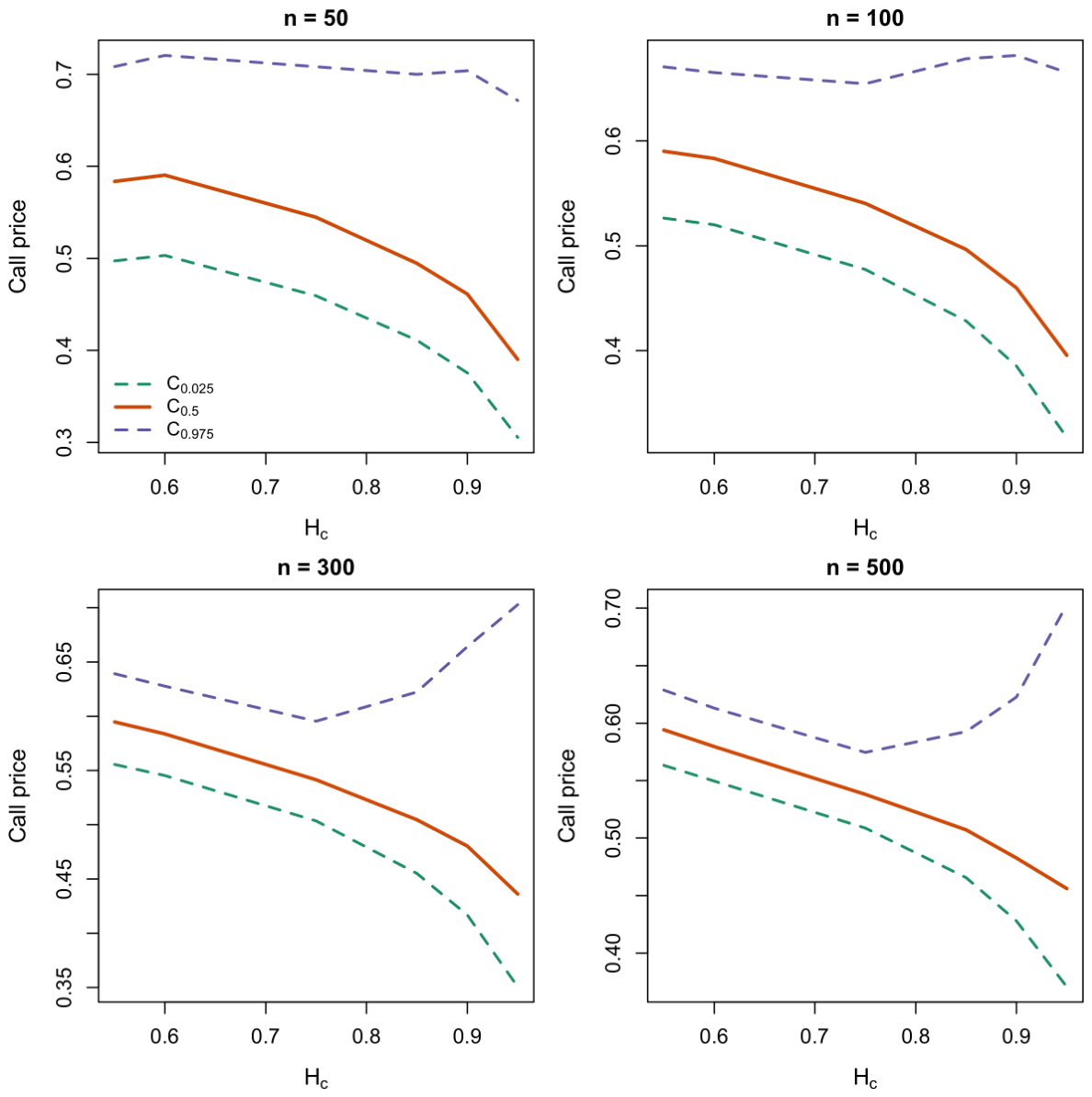
Figure 6.
Joint posterior distribution of the Hurst parameter H and volatility for WTI crude oil across two periods. While H remains concentrated around 0.5, volatility differs substantially between regimes.
Figure 6.
Joint posterior distribution of the Hurst parameter H and volatility for WTI crude oil across two periods. While H remains concentrated around 0.5, volatility differs substantially between regimes.
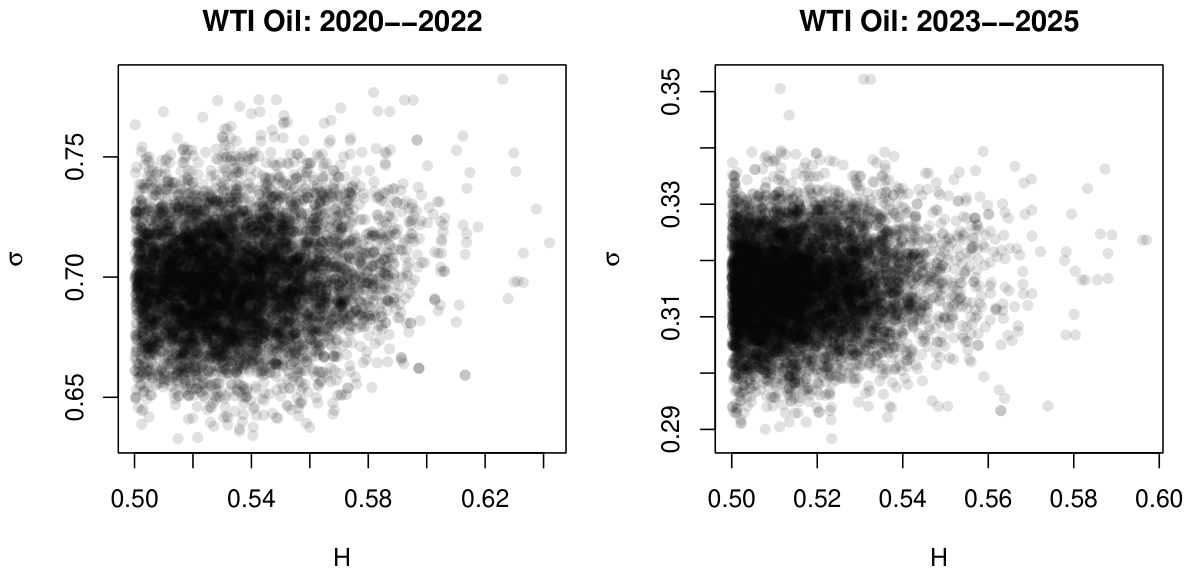
Figure 7.
Posterior distribution of option prices under the fractional Black–Scholes model for WTI crude oil across two periods.
Figure 7.
Posterior distribution of option prices under the fractional Black–Scholes model for WTI crude oil across two periods.
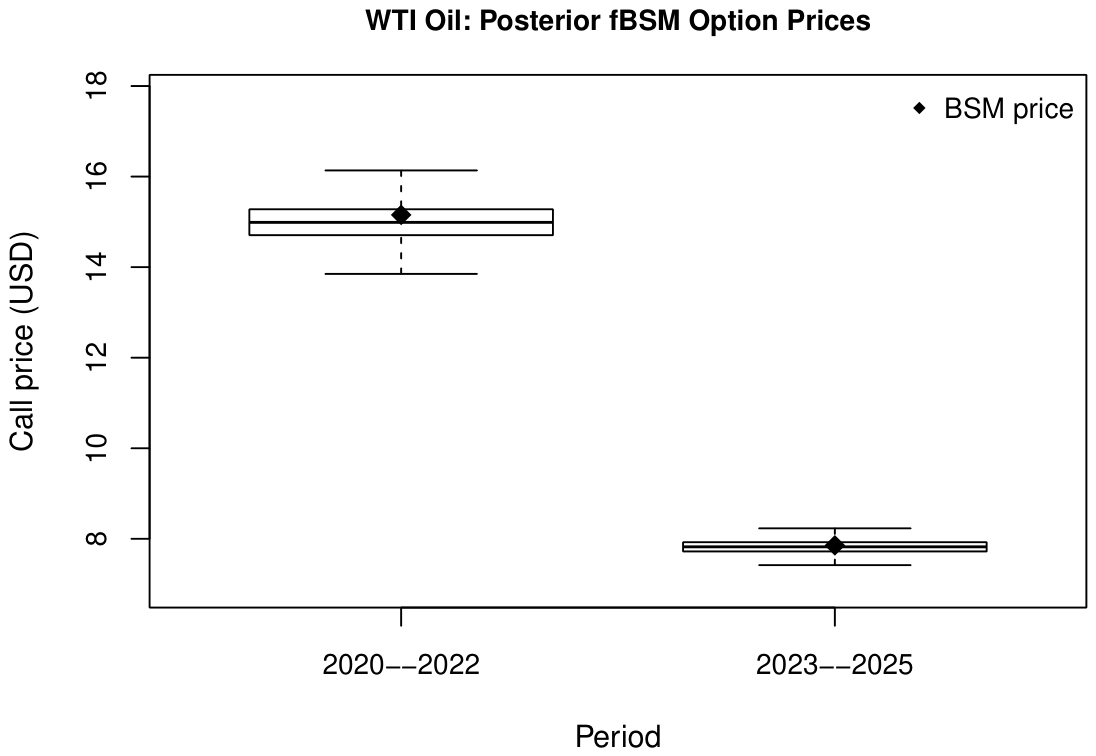
Figure 8.
Joint posterior distribution of the Hurst parameter H and volatility for natural gas. The estimates of H are concentrated around 0.5, while exhibits substantial dispersion.
Figure 8.
Joint posterior distribution of the Hurst parameter H and volatility for natural gas. The estimates of H are concentrated around 0.5, while exhibits substantial dispersion.
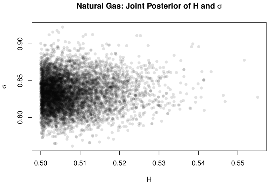
Figure 9.
Posterior distribution of option prices under the fractional Black–Scholes model for natural gas. The Black–Scholes price is shown for comparison.
Figure 9.
Posterior distribution of option prices under the fractional Black–Scholes model for natural gas. The Black–Scholes price is shown for comparison.
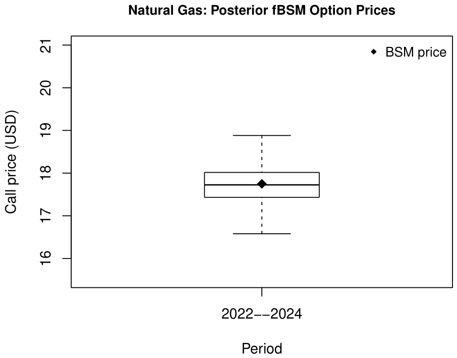
Table 1.
Simulation summary (). Coverage is the empirical proportion of replications where the true pair lies inside the estimated 95% joint HDR. Posterior call-price quantiles are reported in increasing order.
Table 1.
Simulation summary (). Coverage is the empirical proportion of replications where the true pair lies inside the estimated 95% joint HDR. Posterior call-price quantiles are reported in increasing order.
| n | Coverage | Mean H Bias | Mean Bias | Mean Corr | ||||||
|---|---|---|---|---|---|---|---|---|---|---|
| 50 | 0.55 | 0.98 | 0.0617 | 0.0213 | 0.4914 | 0.4974 | 0.5097 | 0.5836 | 0.6840 | 0.7085 |
| 50 | 0.60 | 0.98 | 0.0379 | 0.0495 | 0.5392 | 0.5033 | 0.5153 | 0.5904 | 0.6947 | 0.7206 |
| 50 | 0.75 | 0.99 | -0.0204 | 0.0103 | 0.6613 | 0.4593 | 0.4710 | 0.5447 | 0.6685 | 0.7083 |
| 50 | 0.85 | 0.96 | -0.0541 | -0.0550 | 0.7143 | 0.4110 | 0.4215 | 0.4948 | 0.6471 | 0.7001 |
| 50 | 0.90 | 0.98 | -0.0542 | -0.0970 | 0.7407 | 0.3755 | 0.3857 | 0.4613 | 0.6427 | 0.7040 |
| 50 | 0.95 | 0.98 | -0.0641 | -0.2362 | 0.7440 | 0.3054 | 0.3143 | 0.3901 | 0.6005 | 0.6716 |
| 100 | 0.55 | 0.94 | 0.0250 | 0.0226 | 0.3538 | 0.5243 | 0.5356 | 0.5955 | 0.6561 | 0.6706 |
| 100 | 0.60 | 0.98 | 0.0152 | 0.0265 | 0.4477 | 0.5167 | 0.5293 | 0.5863 | 0.6502 | 0.6652 |
| 100 | 0.75 | 0.96 | 0.0007 | 0.0274 | 0.7076 | 0.4413 | 0.4545 | 0.5456 | 0.6590 | 0.6775 |
| 100 | 0.85 | 0.98 | -0.0182 | -0.0043 | 0.7941 | 0.4092 | 0.4211 | 0.5044 | 0.6503 | 0.6696 |
| 100 | 0.90 | 0.98 | -0.0199 | -0.0314 | 0.8077 | 0.3838 | 0.3956 | 0.4762 | 0.6419 | 0.6664 |
| 100 | 0.95 | 0.99 | -0.0341 | -0.1552 | 0.7962 | 0.3056 | 0.3167 | 0.4141 | 0.5901 | 0.6168 |
| 300 | 0.55 | 0.98 | 0.0081 | -0.0004 | 0.2188 | 0.5534 | 0.5616 | 0.5898 | 0.6318 | 0.6392 |
| 300 | 0.60 | 0.98 | 0.0057 | 0.0113 | 0.3457 | 0.5456 | 0.5511 | 0.5832 | 0.6204 | 0.6278 |
| 300 | 0.75 | 0.94 | -0.0040 | 0.0072 | 0.7310 | 0.4921 | 0.5007 | 0.5380 | 0.5929 | 0.6012 |
| 300 | 0.85 | 0.98 | 0.0006 | 0.0148 | 0.8708 | 0.4496 | 0.4566 | 0.5053 | 0.5814 | 0.5908 |
| 300 | 0.90 | 0.99 | -0.0106 | -0.0102 | 0.8743 | 0.4187 | 0.4259 | 0.4810 | 0.5802 | 0.5904 |
| 300 | 0.95 | 0.95 | -0.0215 | -0.1101 | 0.8526 | 0.3382 | 0.3461 | 0.4283 | 0.5654 | 0.5866 |
| 500 | 0.55 | 0.97 | 0.0010 | 0.0036 | 0.1787 | 0.5644 | 0.5680 | 0.5941 | 0.6229 | 0.6288 |
| 500 | 0.60 | 0.93 | 0.0050 | 0.0065 | 0.3258 | 0.5510 | 0.5541 | 0.5812 | 0.6074 | 0.6131 |
| 500 | 0.75 | 0.96 | 0.0017 | 0.0092 | 0.7437 | 0.4956 | 0.5024 | 0.5371 | 0.5886 | 0.5948 |
| 500 | 0.85 | 0.97 | -0.0054 | -0.0052 | 0.8876 | 0.4427 | 0.4487 | 0.4989 | 0.5719 | 0.5800 |
| 500 | 0.90 | 0.98 | -0.0065 | -0.0024 | 0.9022 | 0.4256 | 0.4302 | 0.4829 | 0.5693 | 0.5773 |
| 500 | 0.95 | 0.98 | -0.0148 | -0.0809 | 0.8774 | 0.3526 | 0.3602 | 0.4379 | 0.5863 | 0.6064 |
Table 2.
Summary statistics for the WTI crude oil return series used in the empirical analysis.
| Asset | Ticker | Period | n | Mean Return | Annualized Volatility |
|---|---|---|---|---|---|
| WTI Crude Oil | CL=F | 2020–2022 | 522 | 0.00185 | 0.696 |
| WTI Crude Oil | CL=F | 2023–2025 | 752 | 0.314 |
Table 3.
Posterior summaries and option pricing results for WTI crude oil across two market periods. The width column represents the length of the 95% posterior credible interval for the fractional Black–Scholes option price.
Table 3.
Posterior summaries and option pricing results for WTI crude oil across two market periods. The width column represents the length of the 95% posterior credible interval for the fractional Black–Scholes option price.
| Period | H (95% CI) | BSM | fBSM (95% CI) | Width | |
|---|---|---|---|---|---|
| 2020–2022 | 0.532 (0.502, 0.586) | 0.698 | 15.15 | 14.99 (14.21, 15.84) | 1.63 |
| 2023–2025 | 0.515 (0.501, 0.551) | 0.315 | 7.86 | 7.82 (7.53, 8.12) | 0.59 |
Table 5.
Posterior summaries and option pricing results for natural gas. The width column represents the length of the 95% posterior credible interval for the fractional Black–Scholes option price.
Table 5.
Posterior summaries and option pricing results for natural gas. The width column represents the length of the 95% posterior credible interval for the fractional Black–Scholes option price.
| Period | H (95% CI) | BSM | fBSM (95% CI) | Width | |
|---|---|---|---|---|---|
| 2022–2024 | 0.505 (0.500, 0.526) | 0.833 | 17.75 | 17.72 (16.94, 18.56) | 1.62 |
Disclaimer/Publisher’s Note: The statements, opinions and data contained in all publications are solely those of the individual author(s) and contributor(s) and not of MDPI and/or the editor(s). MDPI and/or the editor(s) disclaim responsibility for any injury to people or property resulting from any ideas, methods, instructions or products referred to in the content. |
© 2026 by the authors. Licensee MDPI, Basel, Switzerland. This article is an open access article distributed under the terms and conditions of the Creative Commons Attribution (CC BY) license (http://creativecommons.org/licenses/by/4.0/).
Copyright: This open access article is published under a Creative Commons CC BY 4.0 license, which permit the free download, distribution, and reuse, provided that the author and preprint are cited in any reuse.


