

Submitted:
18 June 2026
Posted:
19 June 2026
You are already at the latest version
Abstract
Petroleum, also known as crude oil, is a natural, non-renewable, and essential energy resource. Its extraction and transportation require specific precautions/recommendations to prevent or mitigate potential emergency scenarios, and pollution of soil, air, and water resources. One of the safest ways of transporting crude oil is through pipelines. However, they are subject to corrosion that may lead to leaks that cause severe environmental and water pollution. In this paper, we investigate the migration of petroleum in a scenario mimicking a pipeline leakage (with the pipeline included in the numerical simulation) and the consequent spread of the contaminant in the environment. We use the numerical code CactusHydro, which accurately resolves the sharp discontinuities and temporal dynamics of three-phase fluid flow and thereby accurately tracks contaminant migration in space and time through a variably saturated zone with variable permeability and porosity. We analyze various scenarios encompassing different climatic conditions, including rainfall-induced water saturation, in the variable-saturation porous medium zone and different porosity values, for a total of sixteen transient numerical simulations. Hydraulic conductivity is linked to saturation and provides information on the type of porous soil that facilitates contaminant migration. Also, the porosity can vehicle more or less rapidly its vertical movement in the unsaturated zone. The numerical results show that the vertical migration of the petroleum is primarily driven by the high pressure within the pipeline, since the contaminant has a very limited mobility. Moreover, hydraulic conductivity and porosity play important roles in petroleum migration. Our results suggest that, for crude oil, the distribution of leaked oil may not extend below 2 meters in elevation within 10 days. Our conclusions show that certain types of soil are more adaptable at preventing possible spill migration and can be helpful in constructing pipeline paths that avoid or reduce pollution.
Keywords:
petroleum leakage
; crude oil migration
; LNAPL
; groundwater contamination modeling
; numerical simulations
; variably saturated zones
1. Introduction
Petroleum, also known as crude oil, remains one of the most essential sources of energy. However, because of their non-sustainable and non-renewable nature, petroleum resources eventually deplete, while their extraction or transportation can cause environmental pollution and human health concerns [1,2,3,4,5,6]. Moreover, environmental conditions are crucial to the fate and impact of a crude oil spill [7,8]. Therefore, it is necessary to study ways to safely transport it into the environment [9,10].
Crude oil is classified by geographic location, sulfur content, and API gravity [11], a measure of oil density that indicates whether the crude oil is heavy or light compared to water. If API gravity is greater than 10, then the petroleum floats; if it is less than 10, it sinks. Although most crude oils are light nonaqueous phase liquids (LNAPLs), with densities lower than water, they may contain asphaltenes, which are heavy organic macromolecules classified as dense nonaqueous phase liquids (DNAPLs) [12]. It can also be considered its viscosity, which typically ranges approximately from to , and relies on the values of the American Petroleum Institute (API) gravity and temperature [13],[14]. Usually, to transport crude oil with elevated viscosity through a pipeline, it is necessary to increase the temperature using a hot-pumping method. When pumping is shut down, the system temperature is decreased, and therefore the crude oil viscosity increases [14,15].
Oil seepage and spills are environmental disasters with lasting, harmful effects on marine ecosystems. Recently, the introduction of nanoparticles into contaminated areas to enhance bioremediation of oil spills has emerged as a successful method, especially for marine microorganisms [16,17]. Other oil spills cleanup techniques include mechanical methods using containment booms, and an underflow dam [18], in situ chemical oxidation of petroleum hydrocarbons [19], thermal methods for a rapid recovery of oil and microplastics in marine oil spill co-contamination [20], bioremediation techniques [21] using green composites [22], or natural mineral sorbents as green materials [23]. All these techniques have advantages and disadvantages, as the efficacy of each depends on factors such as viscosity, volume, density, location, and weather conditions [16].
Numerical modeling of crude oil leakage and migration from pipelines and storage facilities is challenging. Risk analysis using different models and numerical methods has been studied for petroleum/crude oil migration due to stress-induced corrosion, corroded ions, and microorganisms [24]. The length of parallel pipelines for transporting petroleum is continuously increasing. Ref. [25] uses numerical simulations to investigate the impact of oil spill and fires accidents nearby natural gas pipelines and indicates that vapor concentration and the size of are the most critical factors. Ref. [26], analyzes the migration from an accidental hole in a tank containing petroleum and the influence of hole diameter, tank height, and tank width. Ref. [27] uses the lattice Boltzmann method to investigate hydrocarbon migration and accumulation and multi-scale quantitative numerical simulation method and a comparison with a sandbox experiment results. Other numerical results include FEM (finite element method) [28] with COMSOL, FDM (finite difference method) [29] investigates BTEX plume using MT3DMS, lattice Boltzmann method [30,31], smooth particle hydrodynamics (SPH) [32].
This paper investigates the influence of hydrogeological features, such as the porosity of the porous medium, and different climatic conditions, including rainfall-induced water saturation, on petroleum migration in the variable-saturated zone. The objective is to select a better location based on its hydrogeological features for the possible construction of onshore petroleum pipelines, as well as to suggest possible technical solutions in designing the pipeline features and give useful information to optimize remediation activities in emergency scenarios. Saturation is linked to hydraulic conductivity and provides information on the type of porous soil that facilitates contaminant migration. Also, porosity can influence the velocity of the vertical migration in the unsaturated zone. We analyze the risk analysis of various scenarios that mimic a pipeline leakage (where the pipeline is included in the numerical simulation) and the consequent spread of the contaminant material in the environment.
We use the numerical CactusHydro code [33,34], that has been validated for several scenarios, in particular, using a sandbox laboratory experiment [35], and various applications including PCE extraction in potential emergency scenarios [36]. The CactusHydro code accurately resolves the sharp discontinuities and temporal dynamics of three-phase fluid flow, thereby accurately tracking contaminant migration in space and time through a variably saturated zone. We present sixteen numerical simulation results that mimic petroleum outflow from a broken pipeline (the most extreme event) and migration toward the saturated zone under the forces of gravity and capillary pressures, to quantify the environmental damage that can be caused over time. Due to its elevated viscosity, crude oil has very limited mobility; for this reason, it migrates very little vertically, and most of it moves under the pressure from the pipeline outflow. The broken pipeline is included in the numerical simulations and modeled as a low-permeability material. Previous investigations using pipelines, but not with petroleum, and with different geometries have been reported in Refs. [37,38].
2. Materials and Methods
2.1. Hydrogeological and Geological Data
In Italy, natural hydrocarbon emissions are mostly located in the Southern Apennine thrust belt [39]. Based on the structural units present in the area and their relative permeabilities, distinct hydrogeological complexes are identified. For example, carbonate complex and high permeability due to fracturing and karst phenomena, and alluvional complex with variable permeability, among others.
We investigate the possible consequences of an emergency scenario in the area where a possible network of onshore pipelines could be constructed to transport crude oil, with hydrogeological features including an alluvial complex and a lithology of alternating clay, gravel, and sand. Currently, comparison with experimental results is not possible because such data are not publicly available. However, this study employs real hydrogeological values consistent with previously described lithological features. Therefore, the results are applicable and reproducible in any region exhibiting similar hydrogeological characteristics.
In this area, a risk analysis is developed to estimate the quantity of petroleum released into the environment in the event of an accidental loss of containment from an onshore pipeline. We are also interested in the time required for crude oil to migrate from the leak site toward the groundwater table, and the quantity of petroleum mass released, under different climate conditions, to plan the time needed to begin possible remediation. Since crude oil has very limited mobility due to its high dynamic viscosity, we are interested in determining the minimum time beyond which crude oil does not reach the groundwater table under various climate conditions, including the dry season and rainfall-induced saturation, for different values of the porous medium’s porosity. We are interested in providing guidelines to minimize the damage of crude oil spills in emergency situations.
2.2. Mathematical Model
For a three-phase immiscible fluid flow composed of nonaqueous (n), i.e., petroleum, water (w), and air (a) in a variably saturated zone, CactusHydro resolves the system of three partial differential equations as a function of the saturations of the three-phase fluid flow, and pressure variables: , , , and . The conservation relation, holds. See Refs. [33,34,37]. The rock compressibility as a function of the porosity and pressure is given by: . We use a linear approximation of this expression, obtained by a Taylor expansion up to order one in . The resulting porosity is given by: , where is the porosity value at the reference pressure (the atmospheric). We use the product of the saturation times the porosity: , , and . The system of equations can be written as (assuming constant density and viscosity for each phase fluid flow),
and
where , and
do not depend on the spatial derivative of the saturation, while
depend on the spatial derivative of the saturation. In the regime of interest, the dominant part is the hyperbolic one (Eq.(3)), and is the one that produces and propagating the shock fronts. Eq.(4) instead, is the parabolic part that depends on the capillary pressures, and it is also responsible for the lateral migration of nonacqueous contaminant. CactusHydro uses a High-Resolution Shock-Capturing (HRSC) flux conservative method [40,41,42] that treats the hyperbolic (advective) part of the flow equations better than other numerical methods. See Refs. [33,34] for details. This technique requires a time step size sufficiently small and for this reason the use of High-Performance Computing (HPC). The numerical code is based on an open source software framework to develop parallel HPC simulation codes called Cactus computational toolkit [43,44,45]. Data are evolved on a cartesian mesh wit six refinement level using Carpet [46,47].
The relative permeabilities, , , and , are given by Parker et al. [48]:
where , and is the total effective liquid saturation, and is the irreducible wetting phase saturation. For the capillary pressure we use the van Genuchten model [49], which for the effective saturation has the following form: , where is the capillary pressure head and , m, and n are model parameters.
2.3. Hydrogeological Features and Crude Oil Parameters
The 3D numerical model investigated in this paper simulates an emergency scenario in which an onshore pipeline transporting high-pressure petroleum ruptures, releasing petroleum into the environment. The system is then turned off after one hour, and the spatial and temporal distribution of the petroleum is examined. Since crude oil has a high viscosity, its mobility is very limited. Therefore, we are interested in defining a temporal window during which the petroleum remains in the unsaturated zone and can be mechanically remediated before reaching the groundwater table. We applied the numerical code CactusHydro, originally introduced in Refs. [33,34], which has been checked and expanded over the years using several different initial and boundary conditions and simulates different scenarios of the petroleum plume migration in a variably saturated zone. We briefly summarized the mathematical model we use, which will help fix notation and clarify parameter notation.
The hydraulic conductivity is considered homogeneous and isotropic in the porous medium, and consistent with the hydrogeological features previously mentioned, and it is given by . Consequently, the permeability k, where , is given by , where is the gravity constant on Earth, is the density of the water, and its dynamic viscosity. The porosity is fixed to , at the reference pressure (the atmospheric, ), and it is compatible with ’sand’ [50]. The rock compressibility, for ’sand’ is given in Ref. [51]. The hydrogeological parameter features are listed in Table 1.
The petroleum crude oil investigated in this work has a density of and an elevated dynamic viscosity, [52] (compared with previous investigations, as for example, for the diesel oil [37], and for the gasoline [38]). The dynamic viscosity limits its displacement, which is why a pressure of is required along the pipeline. The numerical simulation mimics a scenario in which the onshore pipeline is completely broken, and crude oil is released at a pressure of Pascal for 3600 seconds. This is how long it takes to intervene and shut down the pipeline.
The numerical model also includes the broken pipeline (not just the volume cell where the contaminant is ejected), represented as an impermeable parallelepiped with a very low permeability, . We also assumed a hydraulic gradient of 0.01, so that crude oil, as an LNAPL, would remain near the groundwater table and eventually be transported with the flow. In this work, we aim to investigate the time at which remediation can be initiated before the contaminant reaches the groundwater table. We are not interested in letting the crude oil reach the groundwater table, also because the time is very long. In any case, the bottom part of the parallelepiped also has a low permeability, , similar to .
The capillary pressures in Table 1 are calculated from the superficial tensions. The superficial tension air-nonaqueous is [53]. The interfacial tension air-water is [54]. From here we get, , and , where , and (from here, [50]). Using the relation that for three-phase fluid flow only two capillary pressures are independent, we have .
2.4. The Numerical Model, Initial and Boundary Conditions of the Petroleum Leakage
We consider a petroleum leakage with the features given in Table 1 from an onshore pipeline located in a variably saturated zone at one meter depth. We analyze two different initial positions for the petroleum spill: a) , and b) , from the groundwater table surface, which crosses the point . For case a), the grid geometry shown is a parallelepiped with an extension of long from , wide from , and depth from . For case b), the grid geometry shown is a parallelepiped with similar measures in x and y, and a depth of from . The petroleum spill is released with a pressure of for one hour, and has an initial saturation of one, . The remaining vadose zone is at atmospheric pressure. A low permeability zone () is situated between in both cases. We also constructed a real onshore pipeline (depicted in the Figures with light grey) using a low permeability value () that goes from , , and , , for case a). For case b), the onshore pipeline goes from , , and , . Boundary conditions are no-flow, except at the top of the parallelepiped in the infiltration zone.
In this work we performed the following transient numerical simulations of crude oil,
- petroleum spill at from the groundwater table, and in the unsaturated zone,
- petroleum spill at from the groundwater table, and in the unsaturated zone,
- petroleum spill at from the groundwater table, , and initial porosity values in the variably saturated zone.
where these scenarios represent conditions such as dry season (corresponding to zero water saturation), rainfall-induced saturation and different porosities texture.
3. Results and Discussions
In this section, we present the results of sixteen transient numerical simulations of petroleum crude oil migration in a variably saturated zone following a spill from an onshore pipeline. The spill migration is investigated at two different distances from the groundwater table, and . Moreover, the migration of the leaked petroleum is investigated using different values of water saturation in the unsaturated zone to mimic different climatic conditions, , corresponding to different situations starting with dry soil and increasing constant rainfall percolation. The migration of the petroleum spill is also investigated using different values of the porosity in the porous medium, , with constant , and a petroleum spill at .
3.1. 3D Transient Numerical Simulations Results for Water Saturation Values with a Spill Situated at , and
Figure 1 shows the migration of a spilled crude oil at , in a variably saturated zone from an onshore pipeline. The unsaturated zone is dry soil, , and the transient numerical simulations are at different times. The left-hand side shows the 3D numerical saturation contours, , of the three-phase immiscible fluid flow (crude oil, water, air) versus the position, at different times, and corresponds to the plane. The right-hand side instead shows similar results, but in the plane. We show a parallelepiped with dimensions , with a grid spatial resolution of . Zoomed inset on the plane. Color bars on the right state , and . On the left-hand side, the onshore pipeline is depicted in light grey and simulated with a low permeability value (see Table 1).
After the release of petroleum from the onshore pipeline, it moves downward toward the saturated zone due to the gravity force, see Figure 1 a), which shows the migration at . Since petroleum has very limited mobility after 31 days and 8.1 hours, it remains in the unsaturated zone (and has not reached the saturated zone). See Figure 1 b).
A similar behavior happens if the water saturation of the unsaturated zone increases. See for example, Figure 2 with , Figure 3 with , Figure 4 with , Figure 5 with , respectively. They have similar behavior after 204 seconds, see Figure 2 a), Figure 3 a),Figure 4 a), Figure 5 a), and basically the only difference is the water saturation of the unsaturated zone.
In Figure 2 b), the petroleum did not reach the groundwater table after 20 days and 2.2 hours. In Figure 3 b), the petroleum just reaches the groundwater table after 20 days and 6.4 hours. In Figure 4 b), the contaminant arrived at the groundwater table after 18 days and 11.1 hours. In Figure 5 b), the contaminant arrives at the groundwater table after 15 days and 22.7 hours. It seems that the water content (water saturation) in the vadose zone increases the contaminant’s velocity of arrival, even though a smaller quantity of contaminant is released as increases, because water occupies part of the porous medium. The same happens for the right-hand side of each of these figures. Also, the contaminant concentration , decreases as increases. Notice that the right-hand side of each figure is symmetric, since it represents the plane. We will conduct a quantitative study of this issue to determine the mass released in each case.
It is worth noting that the groundwater surface level rises as water saturation increases, since the boundary conditions are held constant in the head. As a result, we observe that petroleum is moving more rapidly toward the groundwater table as the groundwater table rises. From the previous figures, one notices that as far as the water saturation of the unsaturated zone increases, it takes less time for crude oil to arrive near the groundwater table. To resolve this issue, the following subsection presents a migration for a scenario similar to the previous one, but using a spill located 5 meters from the groundwater table.
Table 2,Table 3,Table 4,Table 5,Table 6 show the elevation of the spilled crude oil at the initial position , water saturation , respectively, and different times. The data are the one used for Figure 1,Figure 2,Figure 3,Figure 4,Figure 5, respectively. We show the distribution of the petroleum mass as a function of elevation for different values of and times: 1 hour, 5 hours, 1 day, 5 days, 15 days, etc, and the percentage of trapped contaminant spread all over the space.
Figure 6 shows the elevation as a function of the crude oil mass and the spill at , at fixed water saturation in the unsaturated zone and at different times. To reconstruct the spilled crude oil mass, we use Roe’s Riemann Solver [55] and the data in the previous Table 2,Table 3,Table 4,Table 5,Table 6. Basically, the amount of contaminant initially located on top of the grid slowly moves downward for all values of water saturation in the unsaturated zone.
After 1 hour, the contaminant is almost at the top of the pipeline, and the situation is the same for all values of . As time increases, the contaminant slowly goes downward due to the gravitational force. After 31 days, for , the contaminant has not yet reached the groundwater table, which crosses the point . See Table 2.
For the case and after 15 days (bottom panel), the petroleum has reached the same elevation in meters as in the case after 31 days. This implies that the contaminant is moving downward faster as water saturation in the unsaturated zone increases. See also Table 6. Indeed, for , after 31 days the petroleum has reached the region with a percentage of trapped mass contaminant of 8.93, while for the petroleum reaches the same region with a percentage of trapped mass contaminant of 10.34 just after 15 days.
Figure 7 shows the elevation as a function of the crude oil mass (spill at ) at fixed time and different water-saturation values in the unsaturated zone. Basically, there is no substantial difference in the values of after 1 hour. Similarly, after 5 hours.
For the 5-day and 10-day cases, it is observed that petroleum is moving downward similarly at all saturation values, although its mobility is very limited due to its high viscosity, compared with previous studies using diesel oil [37]. After 15 days, the situation is very similar across all values, but for , the contaminant arrives faster than in the other cases. See the line read in the last panel, which shows a greater quantity of contaminant mass at the elevation of .
3.2. 3D Transient Numerical Simulations Results for Water Saturation Values with a Spill Situated at , and
Let us investigate a similar scenario as before, but using a spilled crude oil situated at instead of . This is to avoid potential interference between the pipeline location and the rising groundwater surface due to rainfall recharge (see Figure 5).
Figure 8 shows the migration of a spilled crude oil at , in a variably saturated zone from an onshore pipeline. The unsaturated zone is dry soil (), and the transient numerical simulations are conducted at different times. The left-hand side shows the 3D numerical saturation contours () of the th three-phase immiscible fluid flow (crude oil, water, air) versus the position, at different times, and corresponds to the plane. The right-hand side, instead, shows similar results but in the plane.
We show a parallelepiped grid with dimensions , with a spatial resolution of . Zoomed inset on the plane. Color bars on the right state , and . On the left-hand side, the onshore pipeline is depicted in light grey along the grid and is simulated with a very low permeability, (see Table 1).
Figure 8 and Figure 1, which differ only in the initial position of the spilled crude oil, are very similar in the contaminant’s spatial and temporal migration. See Table 2, Table 7 for . This result is expected, since the contaminant released from the onshore pipeline does not know the distance to the groundwater surface. After 18 days, the petroleum has moved very little and is far from the groundwater surface.
Figure 9,Figure 10,Figure 11,Figure 12 show similar scenarios with , and , respectively. Since the distance from the spilled contaminant to the groundwater table has increased compared to previous cases, we can now analyze in more detail the impact of vadose-zone water saturation on petroleum mobility. For these figures, we show results for contour saturations of the three-phase fluid flow up to six days. Indeed, after 6 days, the scenario is very similar among the three of them, due to the petroleum’s limited mobility. Nevertheless, it shows that the contaminant moves more easily as increases. See both the left- and right-hand sides of these figures. Also, the contaminant concentration, , decreases as increases. This is because the contaminant can spread more easily when there is water in the unsaturated zone, and fewer contaminant particles occupy the void spaces (which are now occupied by water). Similar situation happens in the case of spill at (see Figure 1, Figure 2, Figure 3, Figure 4 and Figure 5).
Table 7,Table 8,Table 9,Table 10,Table 11, show the elevation of the spilled crude oil at the initial position , water saturation , respectively, and different times. The data are the one used for Figure 8,Figure 9,Figure 10,Figure 11,Figure 12, respectively. We show the distribution of the petroleum mass as a function of elevation for different values of and times: 1 hour, 5 hours, 1 day, 5 days, etc, and the percentage of trapped contaminant spread all over the space.
From the previous tables, we observe that after 5 days and for the range , the spilled contaminant mass is 14.8 Kg and 2.67 % of trapped contaminant; (15.5 Kg, 2.82 %) for ; (17.0 Kg, 3.10 %) for ; (20.4 Kg, 3.74 %) for ; and (22.3 Kg, 4.09 %) for . Moreover, the spilled contaminant mass and the percentage of trapped contaminant mass left after 5 days, in the range is 212.0 Kg and 38.2 % for ; (207.4 Kg, 37.7 %) for , (199.1 Kg, 36.34 %) for ; (196.7 Kg, 35.9 %) for ; and (191.7 Kg, 35.1 %) for . These results suggest that as increases, less contaminant is trapped on top of the grid where the petroleum was released. At the same time, more contaminants are spread in the saturated zone. This suggests that the presence of water (due to rainfall) in the unsaturated zone facilitates the migration of the contaminant toward the saturated zone.
Figure 13 shows the elevation as a function of the crude oil mass at the spill, , at fixed values of in the unsaturated zone and at different times (15 days only for ). To reconstruct the spilled crude oil mass, we use Roe’s Riemann Solver [55] and the data in the previous Table 2, Table 3. Table 4, Table 5, Table 6. For dry soil (), the contaminant is reduced over time. Initially, after 1 hour, the contaminant is almost at the top of the pipeline, and over time, it slowly moves downward due to gravity. After 5 days, the contaminant has not yet reached the groundwater table, even though is increasing. In all scenarios in Figure 13, the contaminant never reaches the groundwater table before 15 days. For (bottom panel), there is more contaminant in the lower part near the saturated zone (see the green line).
Figure 14 shows the elevation as a function of the crude oil mass at , at fixed time values, and for different water-saturation levels in the unsaturated zone. Basically, there is no substantial difference in the value of across the four panels, which correspond to different time intervals (1 hour, 5 hours, 1 day, 5 days). The only difference is noticed in the last panel (after 5 days). Here, we can clearly see that the contaminant is released faster for . See the red line. Also, it arrives downward faster than the other water saturation values. This corroborated the previous figures and data.
3.3. 3D Transient Numerical Simulations Results for Different Initial Porosity Values with a Spill Situated at
Up to here, we were using a fixed initial value of the porosity ( at the atmospheric pressure) given in Table 1, for all the simulations investigated, since we were interested in describing a porous medium composed of ’sand’ with the hydrogeological features described in the section methods and materials.
Let us now investigate the influence on the porosity value for the scenario and a petroleum spill at . The porosity values investigated are , where we included the value (previously shown) to facilitate comparisons, and is the porosity at (the atmospheric pressure).
Figure 15 shows the saturation contours of three immiscible phases (water, crude oil, and air) as a function of position at different times, for an initial porosity of . The first panel shows the initial time , and the second panel shows days and 1.7 hours. As can be seen, the quantity of contaminant mass expelled from the onshore pipeline is smaller than the previous cases with , since there are fewer void spaces in the porous medium. However, it migrates more rapidly toward the groundwater table as it spills out with a very high pressure from the pipeline, and the available space to move is reduced compared to the previous cases with . See Figure 8 for .
Figure 16, Figure 17, Figure 18, and Figure 19 show a similar scenario as before with , but with , respectively. These results suggest that as increases, the amount of expelled contaminant increases, but it moves less. Indeed, the contaminant concentration increases accordingly, as shown in these figures. This is due to its highly dynamic viscosity.
Table 12 refers to data used in Figure 15 with , and Table 13, Table 14, Table 15, Table 16, shows the data used Figure 16 with , Figure 17 with , Figure 18 with , Figure 19 with , respectively. We also include the data in Table 7 for porosity . As can be seen from these data, when the porous medium porosity is very low, such as in Table 12, the spilled contaminant mass, after one hour, and in the range meters is 207.5 Kg and 44.8 % of trapped contaminant. As porosity increases, the amount of petroleum that can be accommodated outside the pipeline increases. See for example, Table 13 for with 235.9 Kg (45.7 %), Table 7 for with 261.0 Kg (46.2 %), Table 14 for with 278.7 Kg (46.4 %), Table 15 for with 294.3 Kg (46.6 %), Table 16 for with 309.9 Kg (46.7 %).
Regarding the migration time, after 5 days, a very small but nonzero quantity of contaminant (0.34 Kg, 0.08 %) arrives in the range m, and (17.4 Kg, 4.2 %) in the range for the porosity value . See Table 12. For the other porosity values the most extended contaminant migration are situated in the range with 0.093 kg for (Table 13); with 0.0006 kg for (Table 7); with 10.64 kg for (Table 14); with 4.47 kg for (Table 15); with 1.51 kg for (Table 16).
Figure 20 shows the z elevation as a function of the spilled petroleum mass at for , different values of the porosities, , and different times. As the porosity increases, the amount of contaminant expelled also increases. This can be clearly seen, for example, in the black line (representing one hour) that runs across all the panels. At the same time, as porosity increases, the contaminant migration velocity decreases, since the upper part empties more quickly for low porosity values, such as and , whereas for higher porosity values the mobility of the contaminant decreases drastically. In a certain sense, the low porosity values force the contaminant, which flows out of the pipeline at very high pressure, to find space as it moves downward. Indeed, for , after 5 days (see the green line), the contaminant quantity is higher than in the other porosity cases, indicating that the contaminant moves at a higher velocity. For the scenarios with , , and , the contaminant discharge is larger than in the previous cases, but its mobility is compromised by the high viscosity. Indeed, these three values are basically similar.
Figure 21 shows the z elevation as a function of the spilled petroleum mass at for , different values of the time, and different porosities, . After one hour (top left panel), it is clearly seen that the biggest quantity of contaminant mass expelled corresponds to the biggest value of the porosity, . This mass decreases with decreasing porosity: . After 5 hours (top-right panel), the contaminant is moving downward due to gravity. The contaminant mass moving more rapidly is the one corresponding to (see the blue line). Similar behavior is confirmed at later times, such as 1 day and 5 days (see bottom panels). That would imply that a low porosity porous medium tends to be contaminated more quickly, although the amount of contaminant is lower than for higher porosity values. This can be used as a recommendation when planning an onshore pipeline: it is better to build an oil pipeline in an area with higher porosity (and/or drier soil) to avoid potential spill migration into the aquifer and reduce water pollution.
3.4. Convergence Study for the Numerical Simulations
The results obtained using CactusHydro and the HRSC method were previously validated in [33,34], using different analytical models, and results from a sandbox experiment [35]. Here, we do not yet have experimental results to compare, since they are not yet available. We have relied on classical convergence tests performed with the same numerical code at different grid resolutions. Figure 22 shows a comparison between results on the saturation contours for petroleum leakage at three different times using two different grid resolutions: and a time step of a),c),e), and and a time step of b),d),f). As can be seen from Figure 22, both results using different times (0.3 hours, 1.0 hour, and 2 days and 8.9 hours are very similar within a error.
4. Conclusions
One of the safest methods of transporting petroleum is through onshore pipelines. However, they are subject to risks such as pipeline corrosion and environmental hazards, which can lead to groundwater pollution and soil poisoning. In this paper, we quantitatively investigate the migration of petroleum in a scenario resembling a broken pipeline (where the pipeline is included in the numerical simulation), and the consequent spread of the contaminant material in the environment.
We use the numerical code CactusHydro, which accurately resolves the sharp discontinuities and temporal dynamics of three-phase fluid flow and thereby accurately tracks contaminant migration in time through a variably saturated zone with variable permeability and porosity. We analyze various scenarios encompassing different climatic conditions, including rainfall-induced water saturation, in the variable-saturation porous medium zone, and different porosity values, for a total of sixteen transient numerical simulations. Hydraulic conductivity is linked to saturation and provides information on the type of porous soil that facilitates contaminant migration. Also, the porosity can convey vertical movement more or less rapidly through the unsaturated zone. The numerical results show that the vertical migration of the petroleum is primarily driven by the high pressure within the pipeline, since the contaminant has a very limited mobility due to its high viscosity. Moreover, hydraulic conductivity and porosity play an important role in petroleum vertical migration. Our results suggest that, for crude oil, the distribution of leaked oil may not extend as deep as two meters in elevation before 10 days.
Our conclusions show that the average seasonal water saturation of the porous medium, its related hydraulic conductivity, and effective porosity must be carefully evaluated when assessing the location of an onshore pipeline and the potential environmental impact of a leak. Our results also suggest that the distribution of leaked petroleum mass for the scenarios investigated may not extend deeper than 2 meters within 10 days. These results may serve as a guideline for constructing an onshore pipeline path that avoids or reduces extreme pollution in a groundwater system.
Our findings on building a sustainable transportation path for petroleum to minimize emergency scenarios include recommendations for constructing a pipeline in a region where a) the aquifer depth is sufficient to protect the groundwater. We find out that constructing a pipeline more than two meters from the groundwater table helps to mechanically remediate the harmful material within a week; b) the characteristics of the soil matrix are important and help to contain the spreading of the crude oil. Indeed, if possible, the choice of constructing a pipeline should prefer a porous medium with lower permeability over one with higher permeability. We have demonstrated that, with a saturation different from zero, crude oil migrates more rapidly downward, as previously reported in other papers using different hydrocarbons [37]. The difference here is that petroleum is highly viscous compared to previous studies, which is good news since its spread is contained. With these recommendations fulfilled, a safer onshore pipeline can be constructed, and in the case of an emergency, less damage is expected.
Author Contributions
Conceptualization, A.F., and F.C.; methodology, A.F.; software, A.F. and M.P.; validation, A.F. and M.P.; formal analysis, A.F.; investigation, A.F.; resources, A.F., and F.C.; data curation, A.F. and M.P.; writing—original draft preparation, A.F.; writing—review and editing, A.F., M.P., and F.C.; visualization, A.F. and M.P. All authors have read and agreed to the published version of the manuscript.
Funding
This research received no external funding.
Institutional Review Board Statement
Not applicable.
Informed Consent Statement
Not applicable.
Data Availability Statement
The original contributions presented in this study are included in the article. Further inquires can be directed to the corresponding author.
Acknowledgments
This work used high-performance computing resources of the University of Parma (https://www.hpc.unipr.it, accessed on 1 January 2025). This research benefited from the equipment and framework of the COMP-R Initiative, funded by the ‘Department of Excellence’ program of the Italian Ministry for the University and Research (MUR 2023-2027). A.F., M.P., and F.C. acknowledge the financial support from: Project funded under the National Recovery and Resilience Plan (NRRP), Mission 4 Component 2 Investment 1.5—Call for Tender No. 3277 of 30/12/2021 of the Italian Ministry of University and Research funded by the European Union—NextGenerationEU. Award Number: Project code ECS00000033, Concession Decree No. 1052 of 23/06/2022 adopted by the Italian Ministry of University and Research, CUP D91B21005370003, “Ecosystem for Sustainable Transition in Emilia-Romagna” (Ecosister).
Conflicts of Interest
The authors declare no conflicts of interest.
References
- United States Environmental Protection Agency. Understanding oil spills and oil spill response. 1999. Available online: https://www.epa.gov/emergency-response/understanding-oil-spills-and-oil-spill-response (accessed on 2026 January 1).
- Hasan, A.M.A.; Nassar, A.M.; Nassar, I.; et al. Environmental impacts for the transportation of crude oil and refined products. Env. Sci. Pollut. Res. Int. 2025, 32, 17869–-17896. [Google Scholar] [CrossRef] [PubMed]
- Fan, K.; Ma, Y.; Li, P.; Yu, C.; Lei, Y.; Li, S.; Zhou, S.; Li, R.; Li, W. Review on Radial Properties of Wax Deposits in Crude Oil Pipelines: Mechanism, Experiment, Property Variation, and Prediction. Energy Fuels 2025, 39(20), 9262–9284. Available online: https://pubs.acs.org/doi/10.1021/acs.energyfuels.5c00484. [CrossRef]
- Zhao, H. J.; Zhang, D.; Lv, X. F.; Song, L. L.; Li, J. W.; Chen, F.; Xie, X. Q. Numerical Simulation of Crude Oil Leakage from Damaged Submarine-Buried Pipeline. J. Appl. Fluid Mech. 2023, 17(1), 75–88. [Google Scholar] [CrossRef]
- Bellegoni, M.; Ovidi, F.; Landucci, G.; Tognotti, L.; Galletti, C. CFD analysis of the influence of a perimeter wall on the natural gas dispersion from an LNG pool. Process Saf. Environ. Prot. 148 2021, 751–764. [CrossRef]
- Kraidi, L.; Shah, R.; Matipa, W.; Borthwick, F. An investigation of mitigating the safety and security risks allied with oil and gas pipeline projects. J. Pipeline Sci. Eng. 1((3) 2021), 349–359. [CrossRef]
- Trainiti, G.M.; Cianelli, D.; Piscopo, V.; Zambianchi, E. Oil spill model in the Gulf of Naples following collision events. Ocean Eng. 2025, 342(3), 123081. [Google Scholar] [CrossRef]
- Nadim, F.; Hoag, G.E.; Liu, S.; Carley, R.J.; Zack, P. Detection and remediation of soil and aquifer systems contaminated with petroleum products: an overview. J. Pet. Sci. Eng. 2000, 26(1–4), 169–178. [Google Scholar] [CrossRef]
- Selva Filho, A.A.P.; Converti, A.; Soares da Silva, R.d.C.F.; Sarubbo, L.A. Biosurfactants as Multifunctional Remediation Agents of Environmental Pollutants Generated by the Petroleum Industry. Energies 2023, 16, 1209. [Google Scholar] [CrossRef]
- Li, H.; Chen, B.; Cao, Y.; Yang, M.; Brydie, J.; Lee, K.; Zhang, B. Wood oil biodegradation in the marine environment: Behavior, mechanism, and impact. Water Res. 2026, 291, 125155. [Google Scholar] [CrossRef] [PubMed]
- Available online: https://en.wikipedia.org/wiki/API_gravity (accessed on 1 January 2026).
- Javanbakht, G.; Lamia Goual, L. Mobilization and micellar solubilization of NAPL contaminants in aquifer rocks. J. Contam. Hydrol. 2016, 185–186, 61–73. [Google Scholar] [CrossRef] [PubMed]
- Gao, X.; Jiang, T.; Li, Y. A Generalized Model for Estimating the Viscosity of Crude Oil. Processes 2025, 13, 1433. [Google Scholar] [CrossRef]
- Bossinov, D.; Ramazanova, G.; Turalina, D. Comparison of measured and calculated high-viscosity crude oil temperature values in a pipeline during continuous pumping and shutdown modes. Int. J. Thermofluid 2024, 24, 10095. [Google Scholar] [CrossRef]
- Flores-Quirino, R.; Pastor-Reyes, O.; Aguayo, J.P.; Ascanio, G.; Méndez, F.; Hernández-Sánchez, J.F.; Sánchez, S. Thermal impact induced by the environment in the transport of heavy oils in offshore insulated pipelines: Evaluation of heat transfer. J. Pet. Sci. Eng. 2022, 2017, 110819. [Google Scholar] [CrossRef]
- Pete, A.J.; Bharti, B.; Benton, M.G. Nano-enhanced Bioremediation for Oil Spills: A Review. ACS ES T Eng. 2021, 1(6), 928–946. [Google Scholar] [CrossRef]
- Dave, D.; Ghaly, A.E. Remediation technologies for marine oil spills: a critical review and comparative analysis. Am. J. Environ. Sci. 2011, 7, 424–440. [Google Scholar] [CrossRef]
- Stanley, M.J.; Timlick, L.; Peters, L.E.; Rodríguez Gil, J.L.; Tomy, G.; Taylor, E.; Havens, S.; Palace, V.P. Rapid Chemical Remediation of Freshwater Enclosures Treated with Conventional Heavy Crude Oil Spills Followed by Enhanced Monitored Natural Recovery. Water 2026, 18, 363. [Google Scholar] [CrossRef]
- Zhang, T.; Zheng, W.; Zhang, N.; Wei, T.; Liu, Y. Efficient in situ chemical oxidation of petroleum hydrocarbons in soil by foaming percarbonate. Chem. Eng. J. 2026, 531, 174166. [Google Scholar] [CrossRef]
- Zhao, C.; Peng, S.; Wu, B.; Kang, L.; Liang, L.; Liu, M.; Yang, L.; Wang, W.; Xu, X. Solar-driven superhydrophobic modified polyurethane sponge for rapid in-situ recovery of oil and microplastics in marine oil spill co-contamination. J. Hazard. Mater. 2025 500, 140470. [Google Scholar] [CrossRef]
- Doshi, B.; Sillanpaa, M.; Kalliola, S. A review of bio-based materials for oil spill treatment. Water Res. 2018, 135, 262–277. [Google Scholar] [CrossRef] [PubMed]
- Ozyurek, S.B.; Soyuer, K.; Ustundag, A. A new approach to remediation of crude oil with promising green composites: Biosurfactant-producing Bacillus sp. consortium entrapped in chitosan, chitosan/glutaraldehyde and chitosan/Na-bentonite. Pet. Sci. 2025, 22(12), 5296–5313. [Google Scholar] [CrossRef]
- Belgibayeva, D.; Aikenova, N.; Abilova, G.; Biktasova, A.; Lepesbayeva, G.; Nazarov, S. Natural Mineral Sorbents as Green Materials for the Remediation of Oil-Contaminated Waters. Processes 2026, 14, 540. [Google Scholar] [CrossRef]
- Wang, C.; Hassanein, M.F.; Li, M. Numerical simulation of oil and gas pipeline corrosion based on single- or coupled-factor modeling: A critical review. Nat. Gas. Ind. B 2023, 10(5), 445–465. [Google Scholar] [CrossRef]
- Guoxi, H.; Xueshuang, Z.; Lu, C.; Yuanjie, H.; Hengyu, L.; et al. Influence of Pressurized Pipeline Leakage and Oil Pool Fires on Parallel Natural Gas Pipelines. Journal of Pipeline Systems Engineering and Practice. Journal of Pipeline Systems Engineering and Practice 2026, 13(1), 04025101. [Google Scholar] [CrossRef]
- Ge, Y.; Huang, W.; Li, X.; Yao, J.; Yang, Q.; Zhang, C.; Kong, X.; Zhou, N. Numerical investigation on oil leakage and migration from the accidental hole of tank wall in oil terminal of pipeline transportation system. J. Pipeline Sci. Eng. 2024, 4(2), 100175. [Google Scholar] [CrossRef]
- Zhao, W.; Jia, C.; Song, Y.; Li, X.; Hou, L.; Jiang, L.; Lu, X. Hydrocarbon migration and accumulation simulation: A review and a novel multi-scale quantitative numerical simulation method. Adv. Colloid Interface Sci. 2025 342, 103523. [Google Scholar] [CrossRef]
- Chen, T.; Zhang, Y.; Dong, Y. Bioremediation experiments and dynamic model of petroleum hydrocarbon contaminated soil. J. Environ. Manag. 2024, 365, 121247. [Google Scholar] [CrossRef] [PubMed]
- Schreiber, M.E.; Carey, G.R.; Feinstein, D.T.; Bahr, J.M. Mechanisms of electron acceptor utilization: implications for simulating anaerobic biodegradation. J. Contam. Hydrol. 2004, 73(1-4), 99–127. [Google Scholar] [CrossRef] [PubMed]
- Jiang, L.; Sun, H.; Li, Z. Lattice Boltzmann flux solver simulation of CO2 displacement in microscale porous media. Fuel 2026, 415, 138411. [Google Scholar] [CrossRef]
- Munarin, F.F.; Gouze, P.; Nepomuceno Filho, F. Two-phase flow dynamics in 3D fractures: Influence of aperture, wettability, and fluid properties from Lattice Boltzmann Simulations. Adv. Water Resour. 2025, 206, 105133. [Google Scholar] [CrossRef]
- Sun, L.; Liu, Y.; Zhu, X.; Wang, Y.; Li, Q.; Li, Z. Multiphase SPH Framework for Oil–Water–Gas Bubbly Flows: Validation, Application, and Extension. Processes 2025, 13, 3922. [Google Scholar] [CrossRef]
- Feo, A.; Celico, F. High-resolution shock-capturing numerical simulations of three-phase immiscible fluids from the unsaturated to the saturated zone. Sci. Rep. 2021, 11, 5212. [Google Scholar] [PubMed]
- Feo, A.; Celico, F. Investigating the migration of immiscible contaminant fluid flow in homogeneous and heterogeneous aquifers with high-precision numerical simulations. PLoS ONE 2022, 17, e0266486. [Google Scholar] [CrossRef] [PubMed]
- Feo, A.; Celico, F.; Zanini, A. Migration of DNAPL in Saturated Porous Media: Validation of High-Resolution Shock-Capturing Numerical Simulations through a Sandbox Experiment. Water 2023, 15, 1471. [Google Scholar] [CrossRef]
- Feo, A.; Pinardi, R.; Artoni, A.; Celico, F. Estimation of Free-Product PCE Distribution in Thick Multilayered Aquifers as Possible Long-Term Pollution Sources for Shallow and Deep Groundwaters, Using High-Precision Numerical Simulations. Water 2024, 16, 3053. [Google Scholar] [CrossRef]
- Feo, A.; Celico, F. Influence of Spill Pressure and Saturation on the Migration and Distribution of Diesel Oil Contaminant in Unconfined Aquifers Using Three-Dimensional Numerical Simulations. Appl. Sci. 2025, 15, 9303. [Google Scholar] [CrossRef]
- Feo, A.; Pinardi, R.; Scanferla, E.; Celico, F. How to Minimize the Environmental Contamination Caused by Hydrocarbon Releases by Onshore Pipelines: The Key Role of a Three-Dimensional Three-Phase Fluid Flow Numerical Model. Water 2023, 15, 1900. [Google Scholar] [CrossRef]
- Remelli, S.; Rizzo, P.; Celico, F.; Menta, C. Natural Surface Hydrocarbons and Soil Faunal Biodiversity: A Bioremediation Perspective. Water 2020, 12, 2358. [Google Scholar] [CrossRef]
- Kurganov, A.; Tadmor, E. New high-resolution central scheme for non-linear conservation laws and convection-diffusion equations. J. Comput. Phys. 2000, 160, 241–282. [Google Scholar]
- Lax, P.; Wendroff, B. Systems of conservation laws. Commun. Pure Appl. Math. 1960, 3, 217–237. [Google Scholar] [CrossRef]
- Hou, T.Y.; LeFloch, P.G. Why nonconservative schemes converge to wrong solutions: Error analysis. Math. Comp. 1994, 62, 497–530. [Google Scholar] [CrossRef]
- Allen, G.; Goodale, T.; Lanfermann, G.; Radke, T.; Rideout, D.; Thornburg, J. Cactus Users’ Guide. 2011. Available online: http://www.cactuscode.org/documentation/UsersGuide.pdf (accessed on 1 January 2025).
- Developers, Cactus. Cactus Computational Toolkit. Available online: http://www.cactuscode.org/ (accessed on 1 January 2025).
- Goodale, T.; Allen, G.; Lanfermann, G.; Massó, J.; Radke, T.; Seidel, E.; Shalf, J. The Cactus Framework and Toolkit: Design and Applications. In High Performance Computing for Computational Science—VECPAR 2002; Springer: Berlin, Germany, 2003. [Google Scholar]
- Schnetter, E.; Hawley, S.H.; Hawke, I. Evolutions in 3D numerical relativity using fixed mesh refinement. Class. Quantum Grav. 2004, 21, 1465–1488. [Google Scholar] [CrossRef]
- Schnetter, E.; Diener, P.; Dorband, E.N.; Tiglio, M. A multi-block infrastructure for three-dimensional time-dependent numerical relativity. Class. Quantum Grav. 2006, 23, S553. [Google Scholar]
- Parker, J.C.; Lenhard, R.J.; Kuppusamy, T. A parametric model for constitutive properties governing multi-phase flow in porous media. Water Resour. Res. 1987, 23, 618–624. [Google Scholar]
- van Genuchten, M.T. A closed form equation for predicting the hydraulic conductivity of unsaturated soils. Soil Sci. Soc. Am. J. 1980, 44, 892–898. [Google Scholar] [CrossRef]
- Carsel, R.F.; Parrish, R.S. Developing joint probability distributions of soil water retention characteristics. Water Resour. Res. 1988, 24, 755–769. [Google Scholar] [CrossRef]
- Freeze, R.A.; Cherry, J.A. Groundwater Book; Prentice-Hall Inc.: Englewood Cliffs, NJ, USA, 1979. [Google Scholar]
- Muñoz, J.A.D.; Ancheyta, J.; Castañeda, L.C. Required Viscosity Values To Ensure Proper Transportation of Crude Oil by Pipeline. Energy Fuels 2016, 30(11), 8850–8854. [Google Scholar] [CrossRef]
- Manara, P.; Bezergianni, S.; Pfisterer, U. Study on phase behavior and properties of binary blends of bio-oil/fossil-based refinery intermediates: A step toward bio-oil refinery integration. Energy Convers. Manag. 2018, 165, 304–315. [Google Scholar] [CrossRef]
- Lam-Maldonado, M.; Aranda-Jiménez, Y.G.; Arvizu-Sanchez, E.; Melo-Banda, J.A.; Díaz-Zavala, N.P.; Pérez-Sánchez, J.F.; Suarez-Dominguez, E.J. Extra heavy crude oil viscosity and surface tension behavior using a flow enhancer and water at different temperatures conditions. Heliyon 2023, 9(2), e12120. [Google Scholar] [CrossRef] [PubMed]
- Roe, P.L. Approximate Riemann solvers, parameter vectors and difference schemes. J. Comput. Phys. 1981, 43, 357–372. [Google Scholar] [CrossRef]
Figure 1.
3D transient numerical simulation results on the saturation contours of three immiscible phases (water, crude oil, and air) vs. the position, at different times. The crude oil is released from the pipeline at in the unsaturated zone with . The grid dimension of has a spatial grid resolution of . (a) ; (b) . The left-hand side shows the plane, and the right-hand side shows the plane. Zoomed inset on the plane. Color bars on the right stand for , and .
Figure 1.
3D transient numerical simulation results on the saturation contours of three immiscible phases (water, crude oil, and air) vs. the position, at different times. The crude oil is released from the pipeline at in the unsaturated zone with . The grid dimension of has a spatial grid resolution of . (a) ; (b) . The left-hand side shows the plane, and the right-hand side shows the plane. Zoomed inset on the plane. Color bars on the right stand for , and .
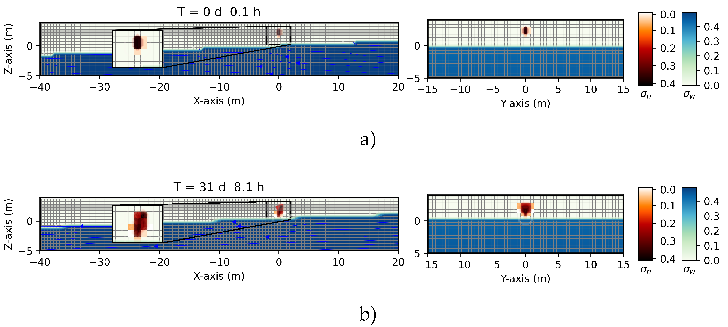
Figure 2.
3D transient numerical simulation results on the saturation contours of three immiscible phases (water, crude oil, and air) vs. position, at different times. The crude oil is released from the pipeline at in the unsaturated zone with . The grid dimension of has a spatial grid resolutio of . (a) ; (b) . The left-hand side shows the plane, and the right-hand side shows the plane. Zoomed inset on the plane. Color bars on the right stand for , and .
Figure 2.
3D transient numerical simulation results on the saturation contours of three immiscible phases (water, crude oil, and air) vs. position, at different times. The crude oil is released from the pipeline at in the unsaturated zone with . The grid dimension of has a spatial grid resolutio of . (a) ; (b) . The left-hand side shows the plane, and the right-hand side shows the plane. Zoomed inset on the plane. Color bars on the right stand for , and .
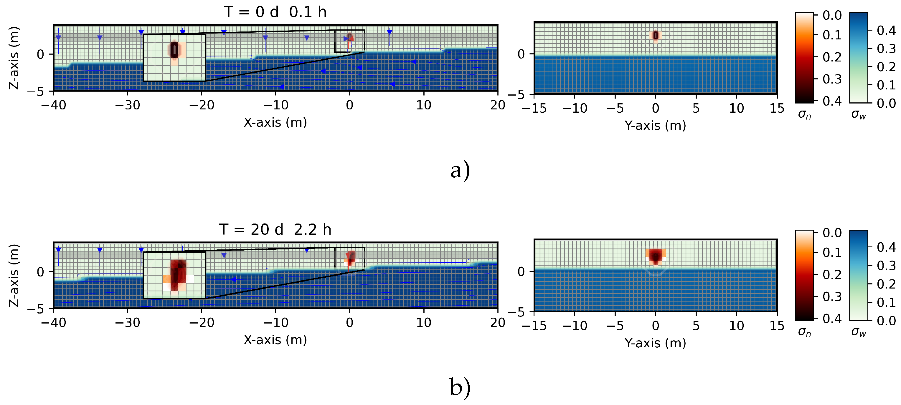
Figure 3.
3D transient numerical simulation results on the saturation contours of three immiscible phases (water, crude oil, and air) vs. the position, at different times. The crude oil is released from the pipeline at in the unsaturated zone with . The grid dimension of has a spatial grid resolution of . (a) ; (b) . The left-hand side shows the plane, and the right-hand side shows the plane. Zoomed inset on the plane. Color bars on the right stand for , and .
Figure 3.
3D transient numerical simulation results on the saturation contours of three immiscible phases (water, crude oil, and air) vs. the position, at different times. The crude oil is released from the pipeline at in the unsaturated zone with . The grid dimension of has a spatial grid resolution of . (a) ; (b) . The left-hand side shows the plane, and the right-hand side shows the plane. Zoomed inset on the plane. Color bars on the right stand for , and .
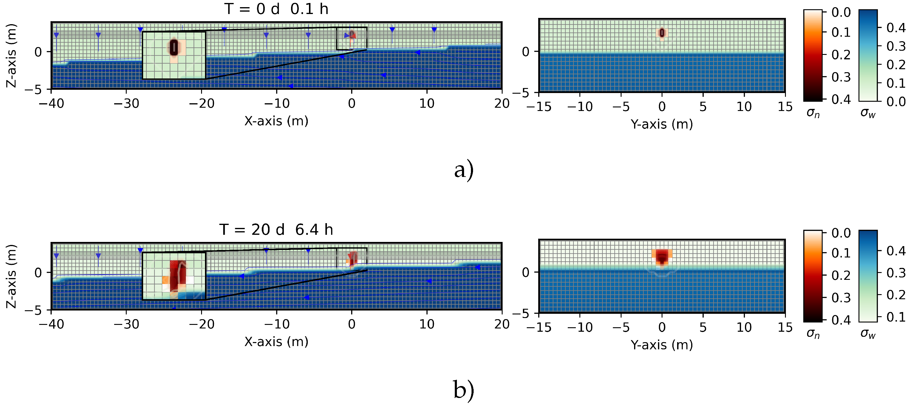
Figure 4.
3D transient numerical simulation results on the saturation contours of three immiscible phases (water, crude oil, and air) vs. the position, at different times. The crude oil is released from the pipeline at in the unsaturated zone with . The grid dimension of has a spatial grid resolution of . (a) ; (b) . The left-hand side shows the plane, and the right-hand side shows the plane. Zoomed inset on the plane. Color bars on the right stand for , and .
Figure 4.
3D transient numerical simulation results on the saturation contours of three immiscible phases (water, crude oil, and air) vs. the position, at different times. The crude oil is released from the pipeline at in the unsaturated zone with . The grid dimension of has a spatial grid resolution of . (a) ; (b) . The left-hand side shows the plane, and the right-hand side shows the plane. Zoomed inset on the plane. Color bars on the right stand for , and .
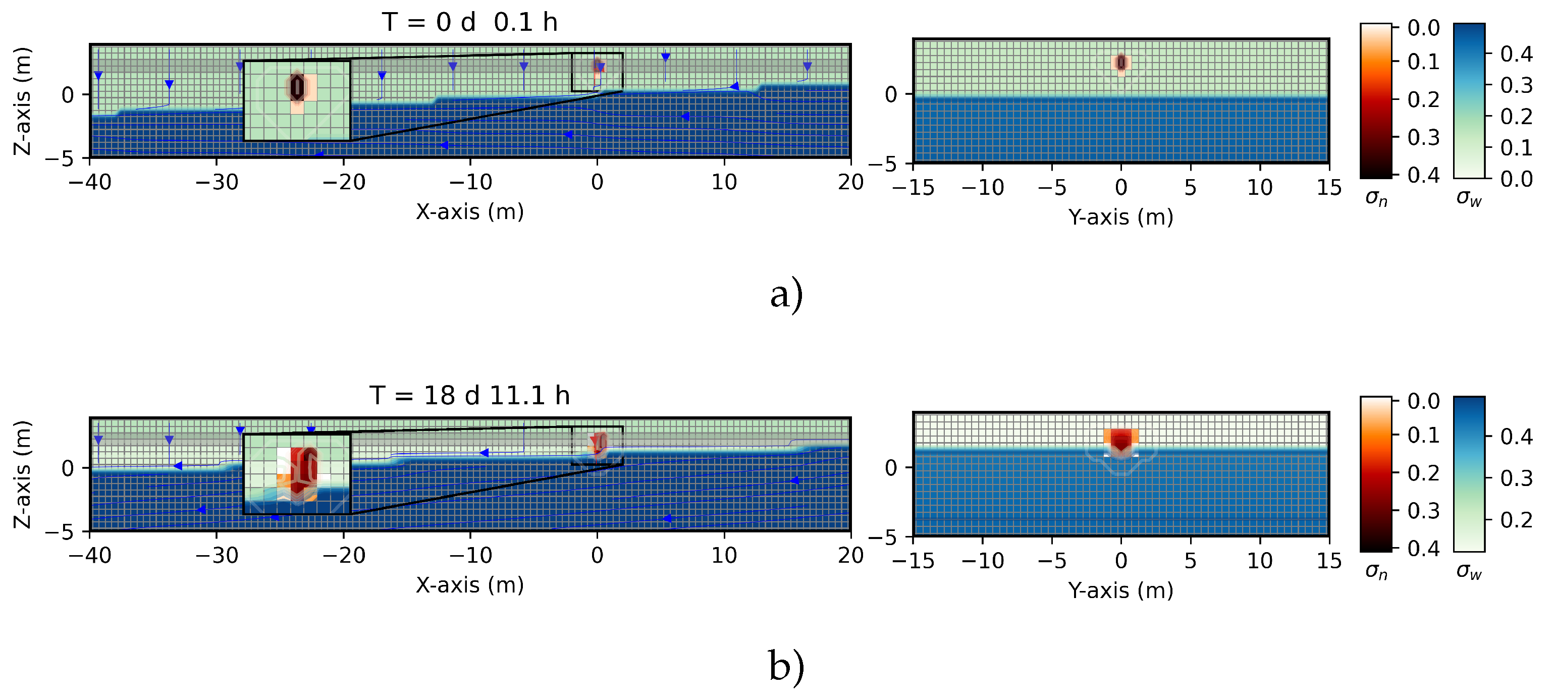
Figure 5.
3D transient numerical simulation results on the saturation contours of three immiscible phases (water, crude oil, and air) vs. the position, at different times. The crude oil is released from the pipeline at in the unsaturated zone with . The grid dimension of has a spatial grid resolution of . (a) ; (b) . The left-hand side shows the plane, and the right-hand side shows the plane. Zoomed inset on the plane. Color bars on the right stand for , and .
Figure 5.
3D transient numerical simulation results on the saturation contours of three immiscible phases (water, crude oil, and air) vs. the position, at different times. The crude oil is released from the pipeline at in the unsaturated zone with . The grid dimension of has a spatial grid resolution of . (a) ; (b) . The left-hand side shows the plane, and the right-hand side shows the plane. Zoomed inset on the plane. Color bars on the right stand for , and .
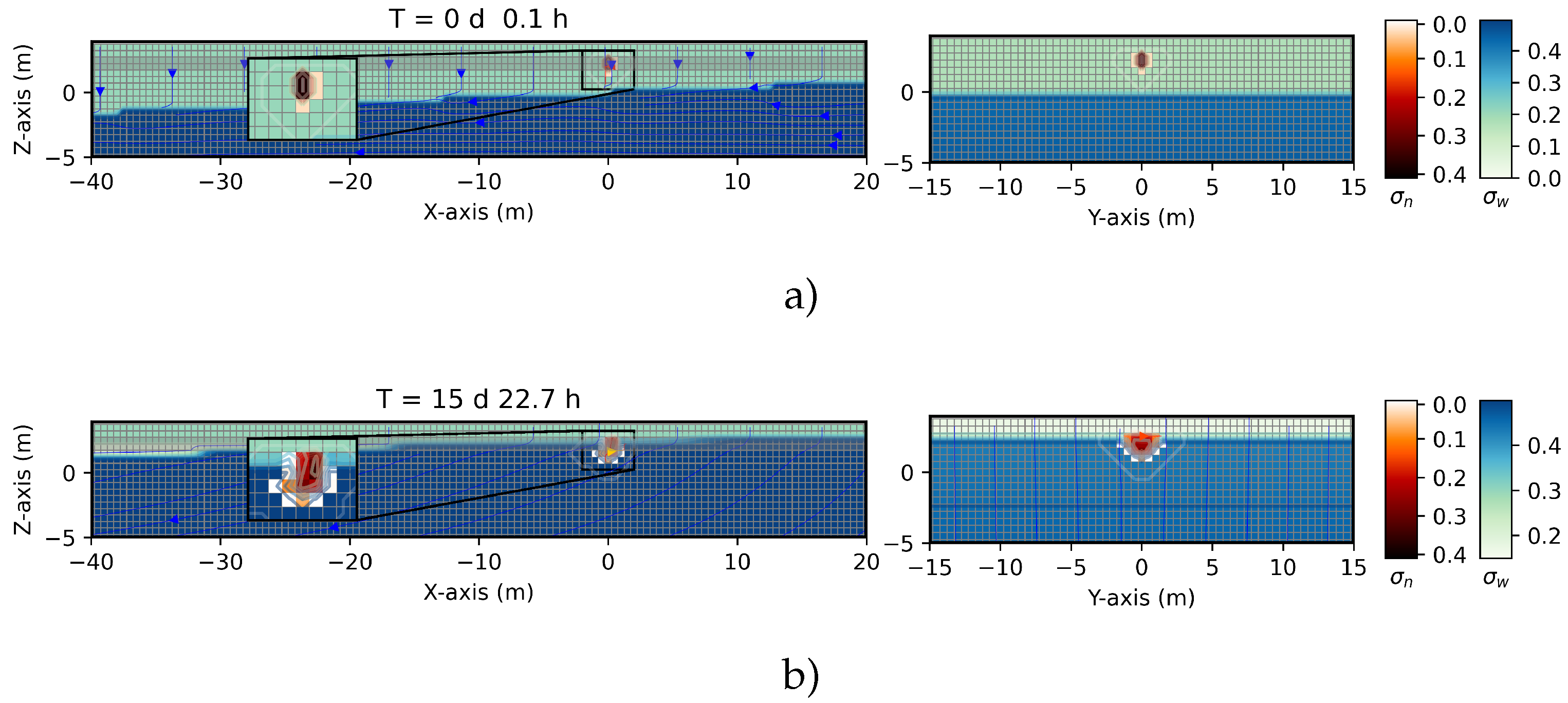
Figure 6.
Elevation vs. crude oil mass spilled at for a fixed value of the water saturation, , and different times.
Figure 6.
Elevation vs. crude oil mass spilled at for a fixed value of the water saturation, , and different times.
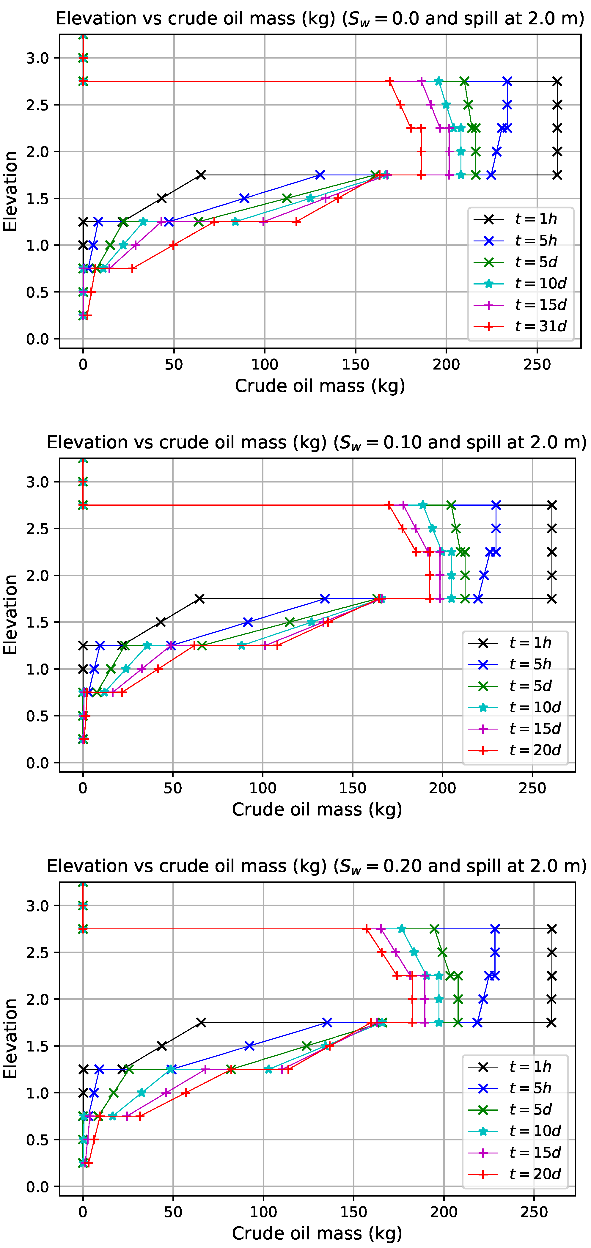
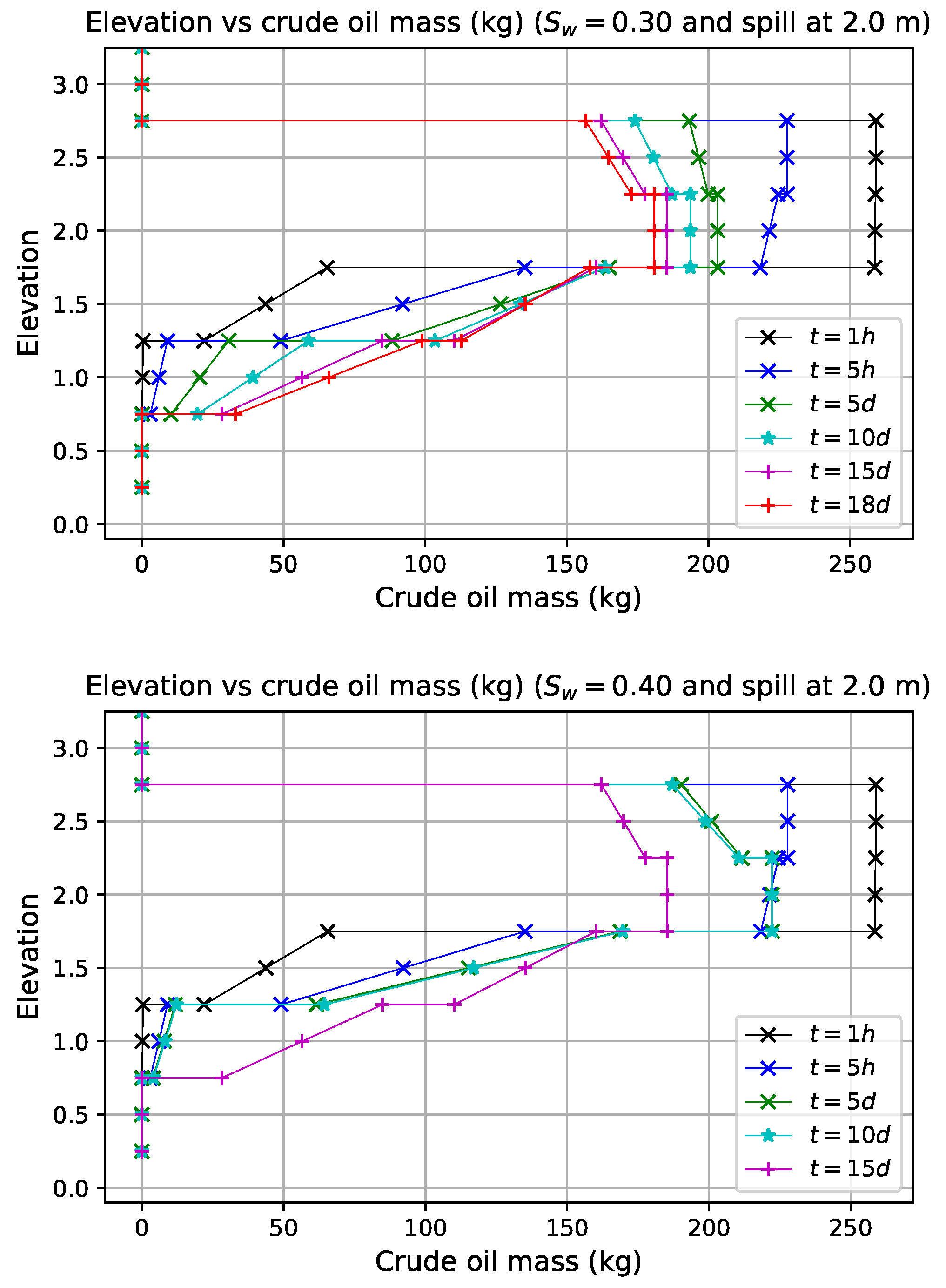
Figure 7.
Elevation vs. crude oil mass spilled at for a fixed value of the time, and different values of the water saturation, .
Figure 7.
Elevation vs. crude oil mass spilled at for a fixed value of the time, and different values of the water saturation, .
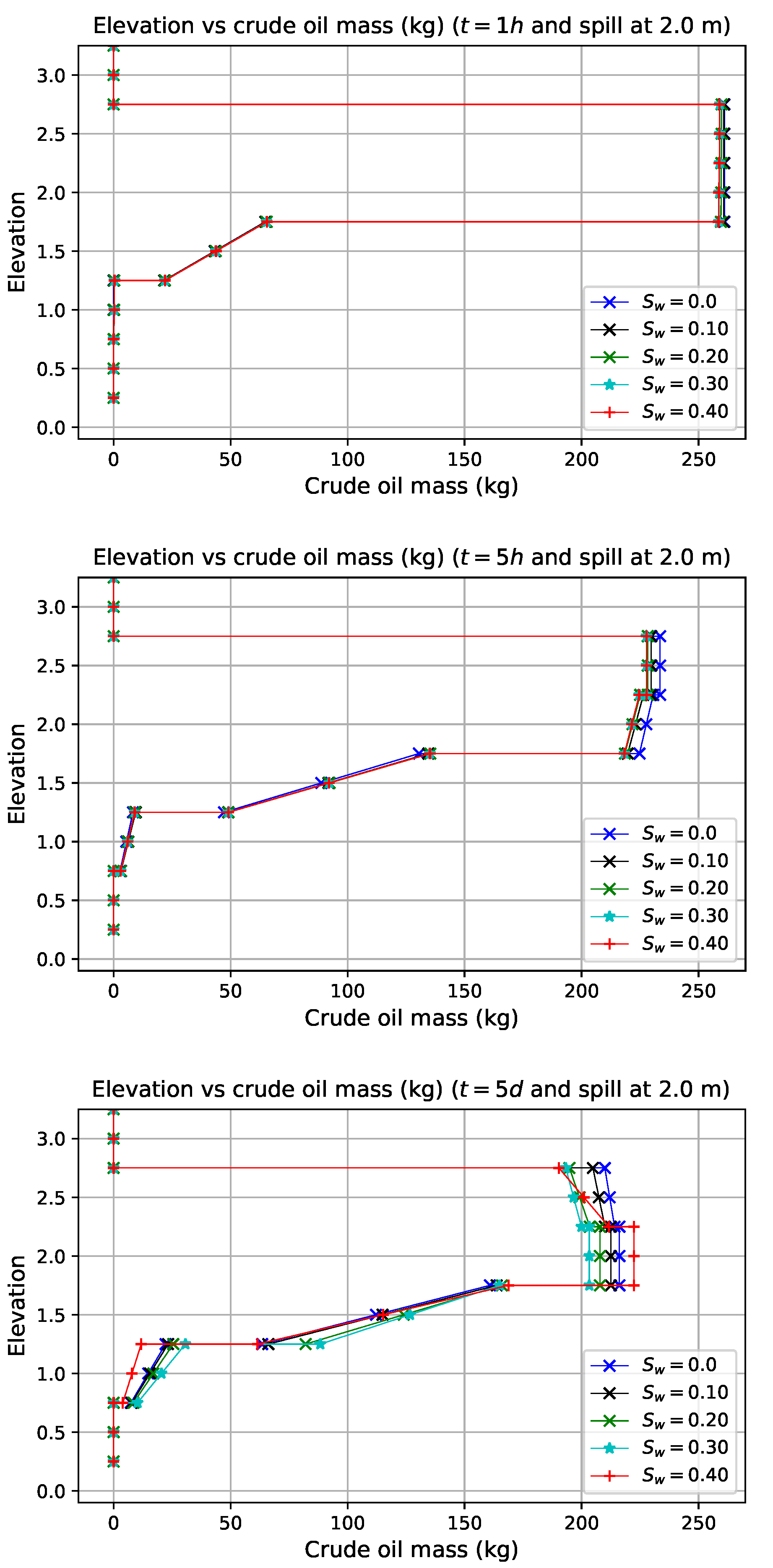
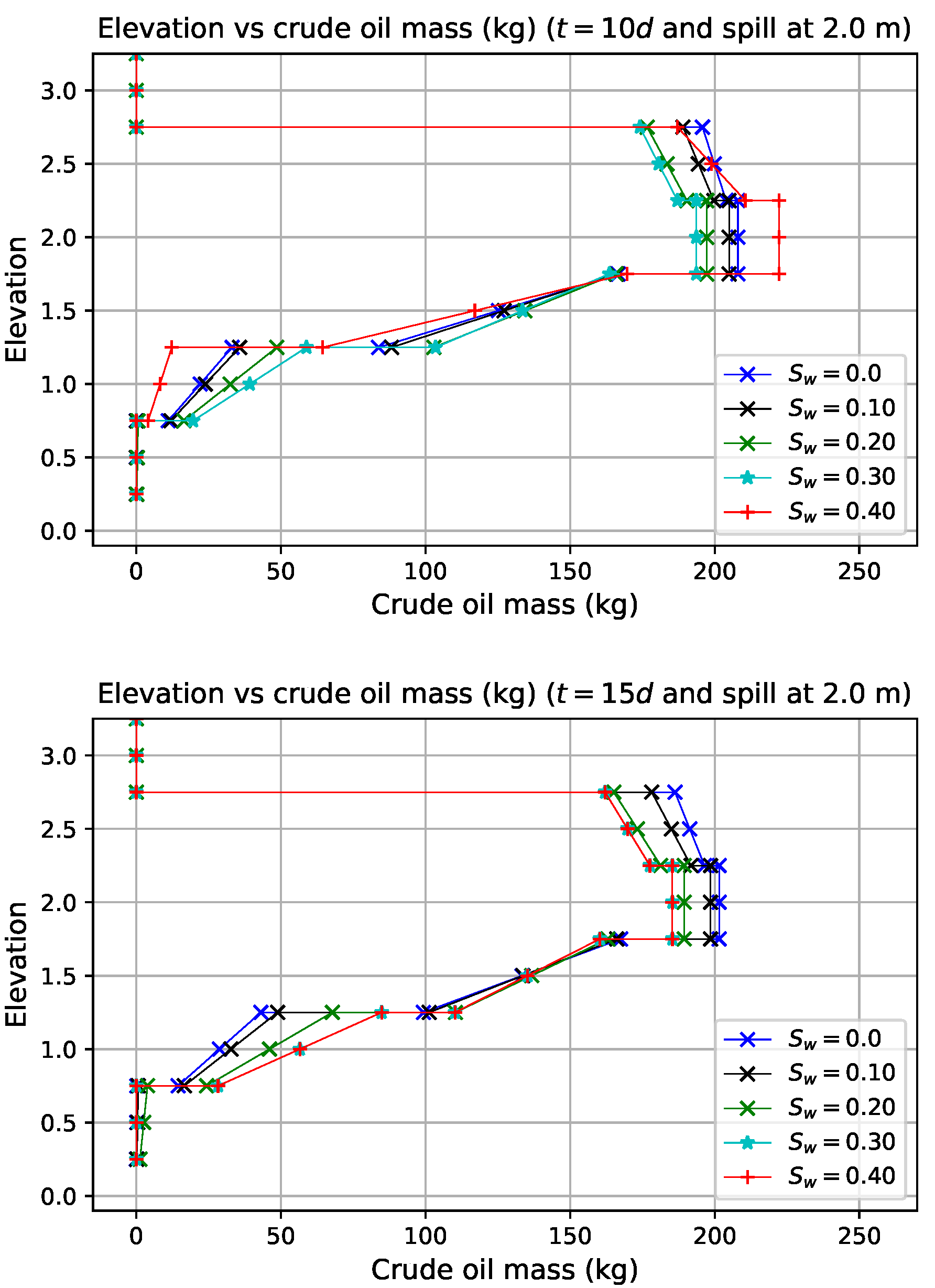
Figure 8.
3D transient numerical simulation results on the saturation contours of three immiscible phases (water, crude oil, and air) vs. the position, at different times. The crude oil is released from the pipeline at in the unsaturated zone with . The grid dimension of has a spatial grid resolution of . (a) ; (b) . The left-hand side shows the plane, and the right-hand side shows the plane. Zoomed inset on the plane. Color bars on the right stand for , and .
Figure 8.
3D transient numerical simulation results on the saturation contours of three immiscible phases (water, crude oil, and air) vs. the position, at different times. The crude oil is released from the pipeline at in the unsaturated zone with . The grid dimension of has a spatial grid resolution of . (a) ; (b) . The left-hand side shows the plane, and the right-hand side shows the plane. Zoomed inset on the plane. Color bars on the right stand for , and .
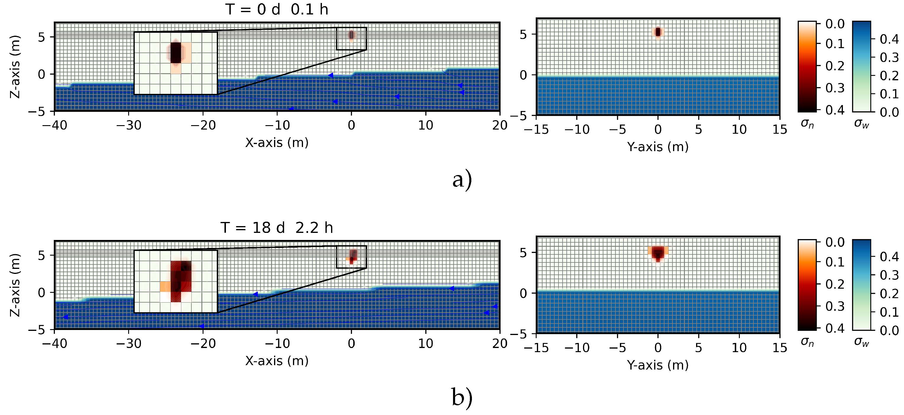
Figure 9.
3D transient numerical simulation results on the saturation contours of three immiscible phases (water, crude oil, and air) vs. the position, at different times. The crude oil is released from the pipeline at in the unsaturated zone with . The grid dimension of has a spatial grid resolution of . (a) ; (b) . The left-hand side shows the plane, and the right-hand side shows the plane. Zoomed inset on the plane. Color bars on the right stand for , and .
Figure 9.
3D transient numerical simulation results on the saturation contours of three immiscible phases (water, crude oil, and air) vs. the position, at different times. The crude oil is released from the pipeline at in the unsaturated zone with . The grid dimension of has a spatial grid resolution of . (a) ; (b) . The left-hand side shows the plane, and the right-hand side shows the plane. Zoomed inset on the plane. Color bars on the right stand for , and .
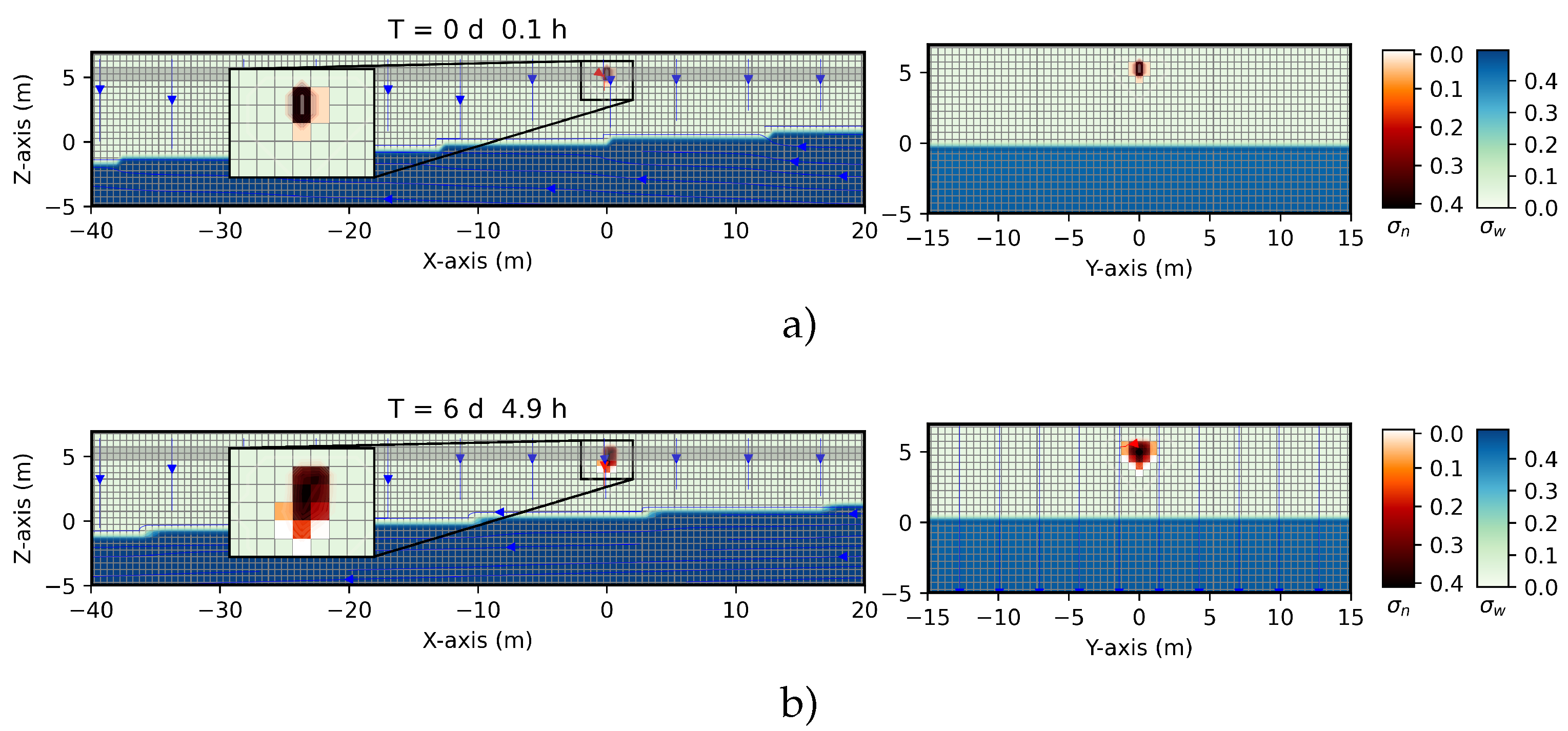
Figure 10.
3D transient numerical simulation results on the saturation contours of three immiscible phases (water, crude oil, and air) vs. the position, at different times. The crude oil is released from the pipeline at in the unsaturated zone with . The grid dimension of has a spatial grid resolution of . (a) ; (b) . The left-hand side shows the plane, and the right-hand side shows the plane. Zoomed inset on the plane. Color bars on the right stand for , and .
Figure 10.
3D transient numerical simulation results on the saturation contours of three immiscible phases (water, crude oil, and air) vs. the position, at different times. The crude oil is released from the pipeline at in the unsaturated zone with . The grid dimension of has a spatial grid resolution of . (a) ; (b) . The left-hand side shows the plane, and the right-hand side shows the plane. Zoomed inset on the plane. Color bars on the right stand for , and .
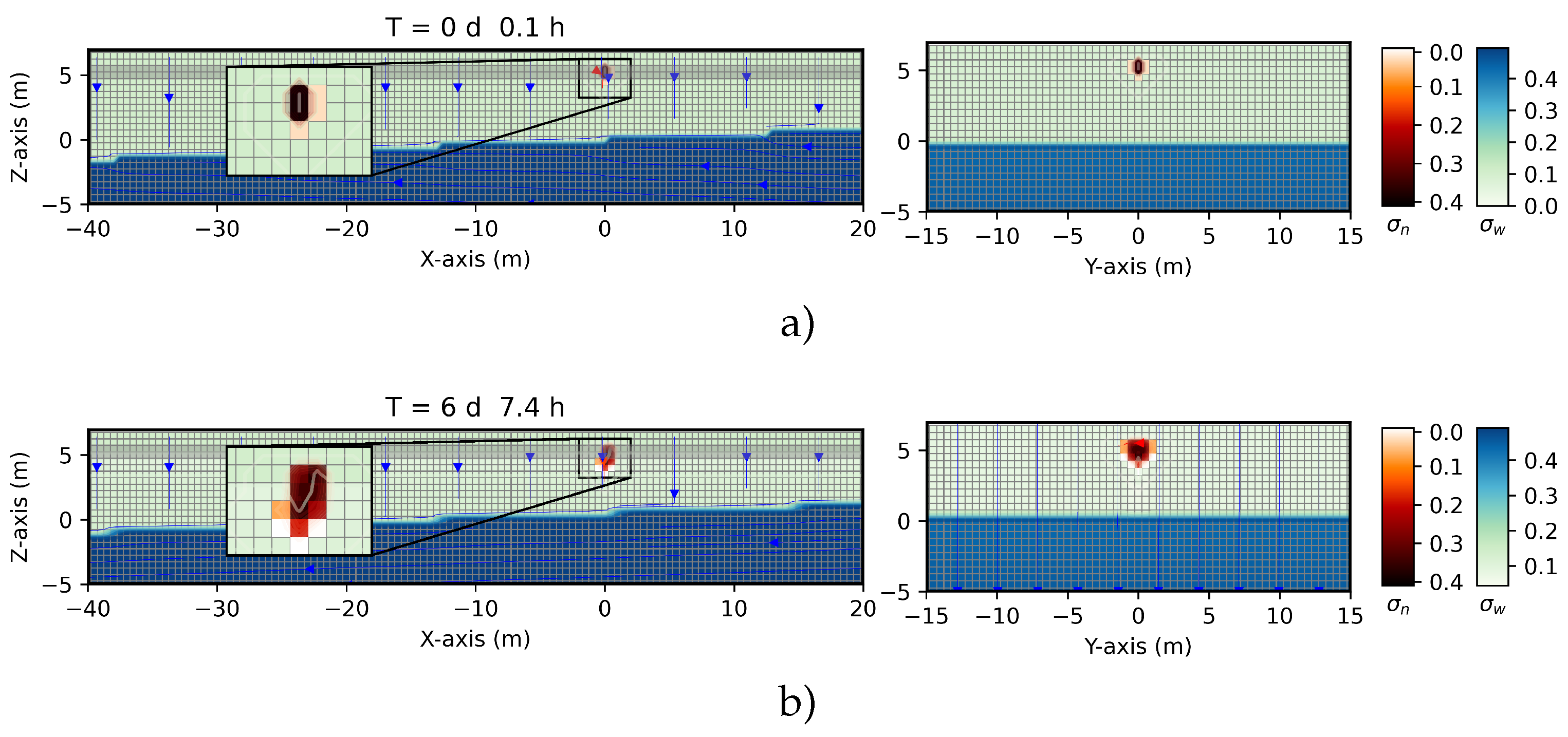
Figure 11.
3D transient numerical simulation results on the saturation contours of three immiscible phases (water, crude oil, and air) vs. the position, at different times. The crude oil is released from the pipeline at in the unsaturated zone with . The grid dimension of has a spatial grid resolution of . (a) ; (b) . The left-hand side shows the plane, and the right-hand side shows the plane. Zoomed inset on the plane. Color bars on the right stand for , and .
Figure 11.
3D transient numerical simulation results on the saturation contours of three immiscible phases (water, crude oil, and air) vs. the position, at different times. The crude oil is released from the pipeline at in the unsaturated zone with . The grid dimension of has a spatial grid resolution of . (a) ; (b) . The left-hand side shows the plane, and the right-hand side shows the plane. Zoomed inset on the plane. Color bars on the right stand for , and .
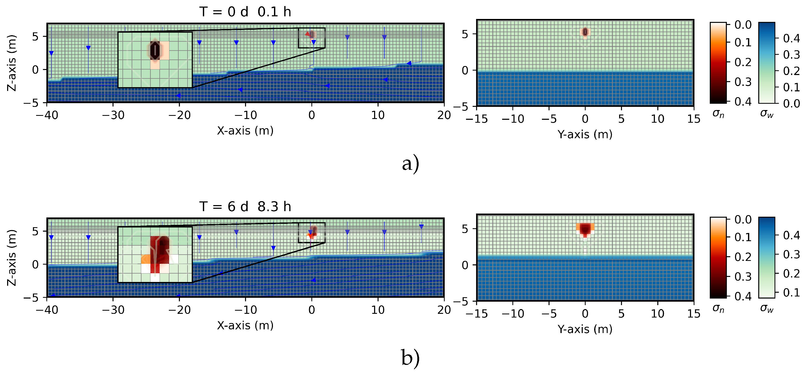
Figure 12.
3D transient numerical simulation results on the saturation contours of three immiscible phases (water, crude oil, and air) vs. the position, at different times. The crude oil is released from the pipeline at in the unsaturated zone with . The grid dimension of has a spatial grid resolution of . (a) ; (b) . The left-hand side shows the plane, and the right-hand side shows the plane. Zoomed inset on the plane. Color bars on the right stand for , and .
Figure 12.
3D transient numerical simulation results on the saturation contours of three immiscible phases (water, crude oil, and air) vs. the position, at different times. The crude oil is released from the pipeline at in the unsaturated zone with . The grid dimension of has a spatial grid resolution of . (a) ; (b) . The left-hand side shows the plane, and the right-hand side shows the plane. Zoomed inset on the plane. Color bars on the right stand for , and .
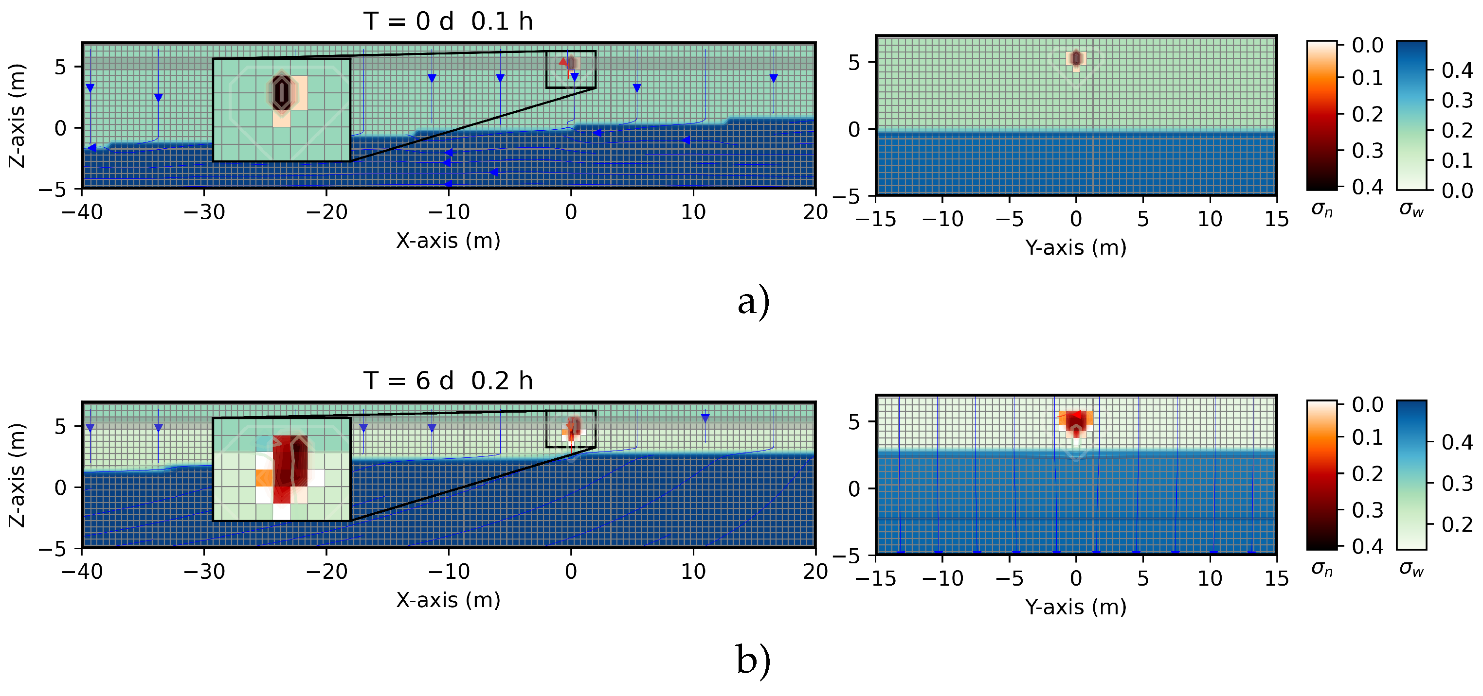
Figure 13.
Elevation vs. crude oil mass spilled at for a fixed value of the water saturation, , and different times.
Figure 13.
Elevation vs. crude oil mass spilled at for a fixed value of the water saturation, , and different times.
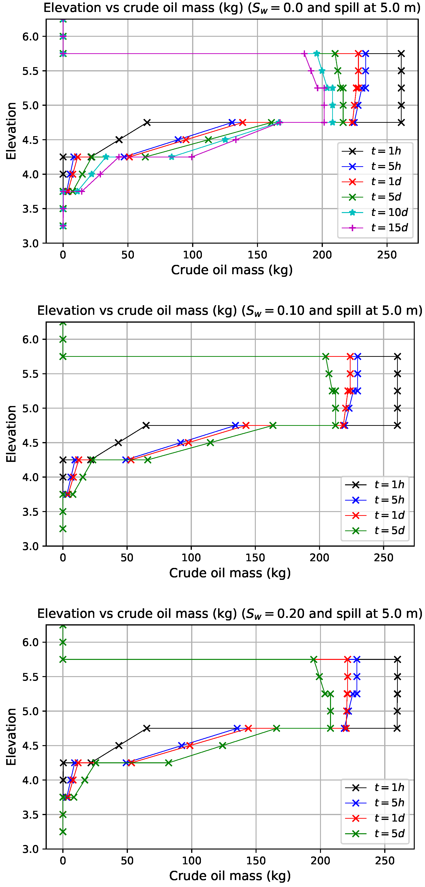
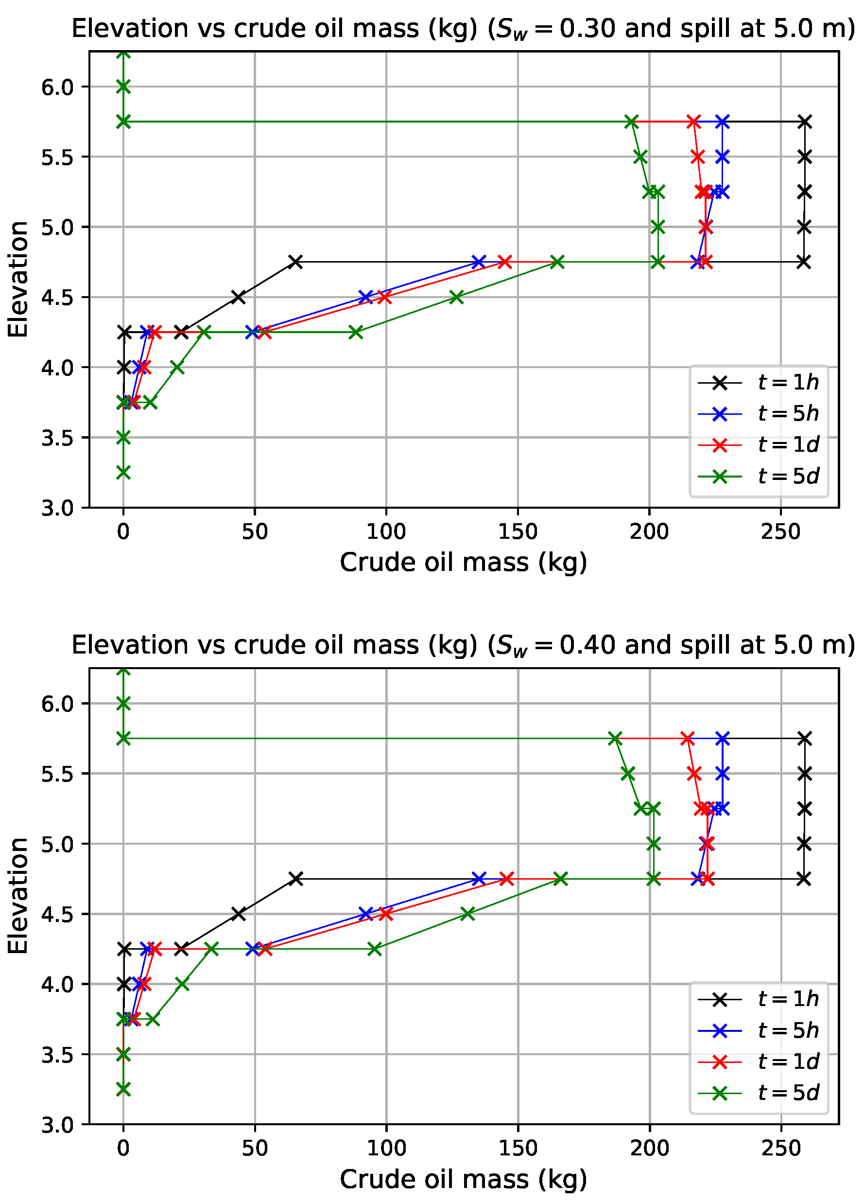
Figure 14.
Elevation vs. crude oil mass spilled at for a fixed value of the time, and different values of the water saturation, .
Figure 14.
Elevation vs. crude oil mass spilled at for a fixed value of the time, and different values of the water saturation, .
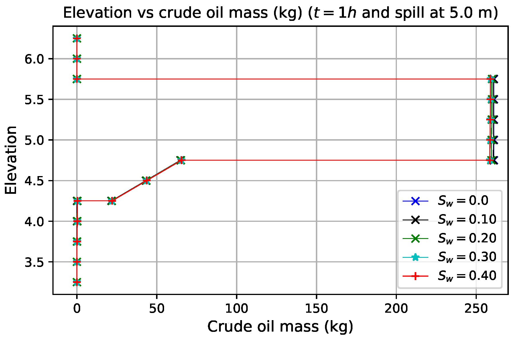
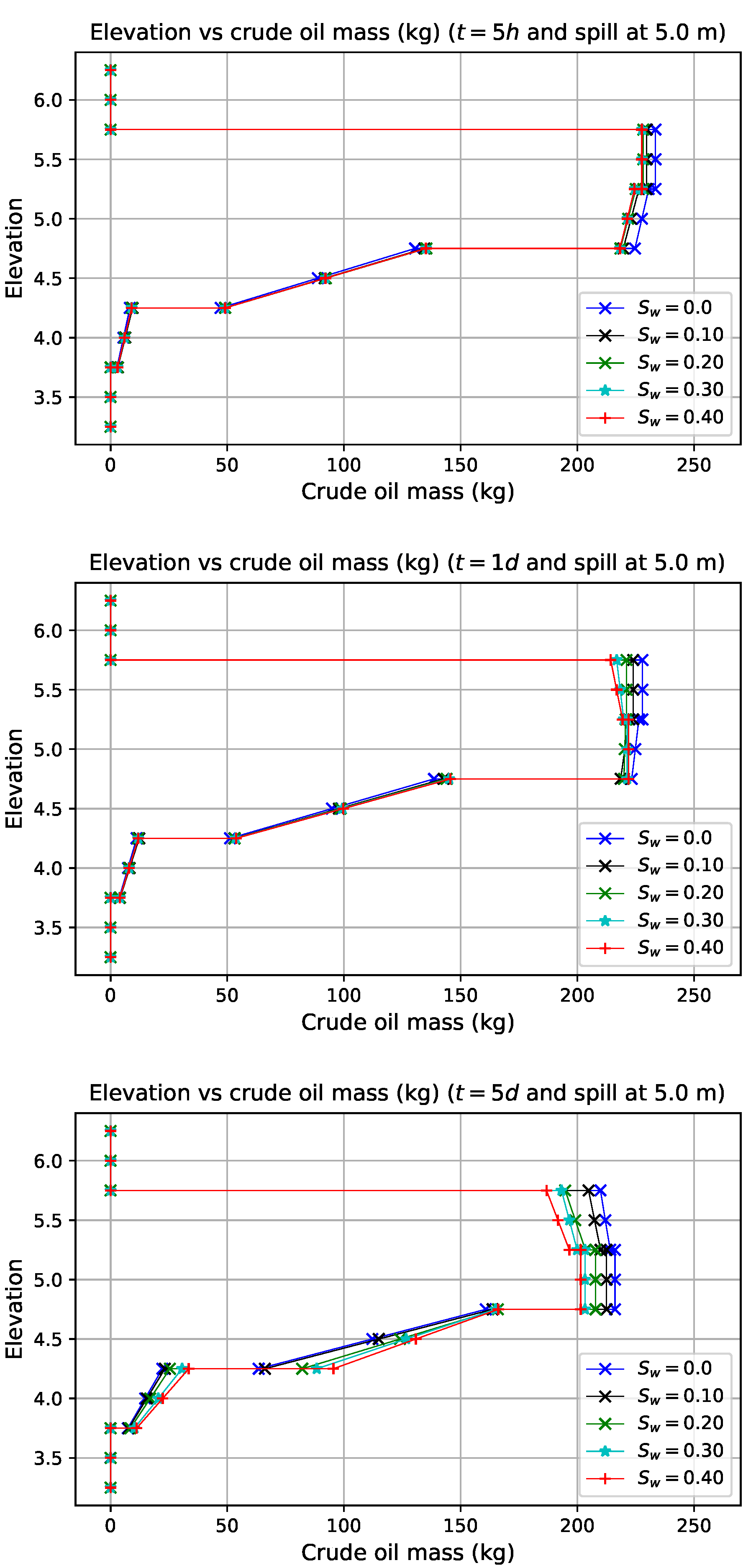
Figure 15.
3D transient numerical simulation results on the saturation contours of three immiscible phases (water, crude oil, and air) vs. the position, at different times. The crude oil is released from the pipeline at in the unsaturated zone with . Porosity value at the atmosphere pressure . (a) ; (b) . The left-hand side shows the plane, and the right-hand side shows the plane. Zoomed inset on the plane. Color bars on the right stand for , and .
Figure 15.
3D transient numerical simulation results on the saturation contours of three immiscible phases (water, crude oil, and air) vs. the position, at different times. The crude oil is released from the pipeline at in the unsaturated zone with . Porosity value at the atmosphere pressure . (a) ; (b) . The left-hand side shows the plane, and the right-hand side shows the plane. Zoomed inset on the plane. Color bars on the right stand for , and .
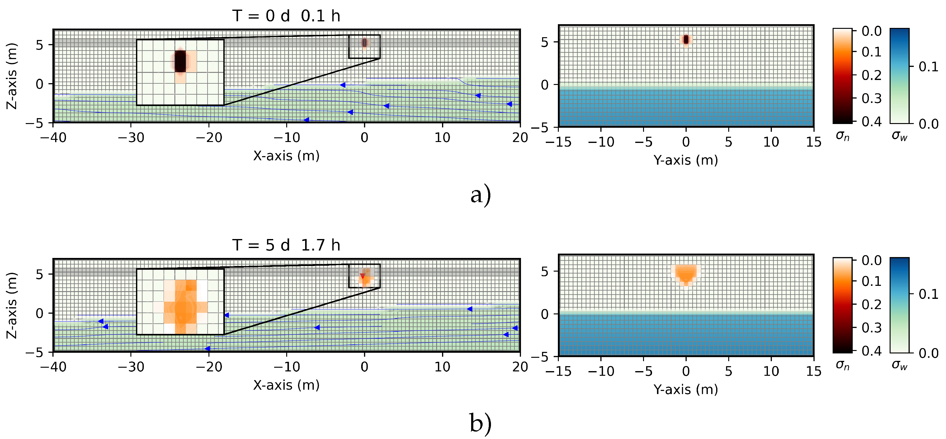
Figure 16.
3D transient numerical simulation results on the saturation contours of three immiscible phases (water, crude oil, and air) vs. the position, at different times. The crude oil is released from the pipeline at in the unsaturated zone with . Porosity value at the atmosphere pressure . (a) ; (b) . The left-hand side shows the plane, and the right-hand side shows the plane. Zoomed inset on the plane. Color bars on the right stand for , and .
Figure 16.
3D transient numerical simulation results on the saturation contours of three immiscible phases (water, crude oil, and air) vs. the position, at different times. The crude oil is released from the pipeline at in the unsaturated zone with . Porosity value at the atmosphere pressure . (a) ; (b) . The left-hand side shows the plane, and the right-hand side shows the plane. Zoomed inset on the plane. Color bars on the right stand for , and .
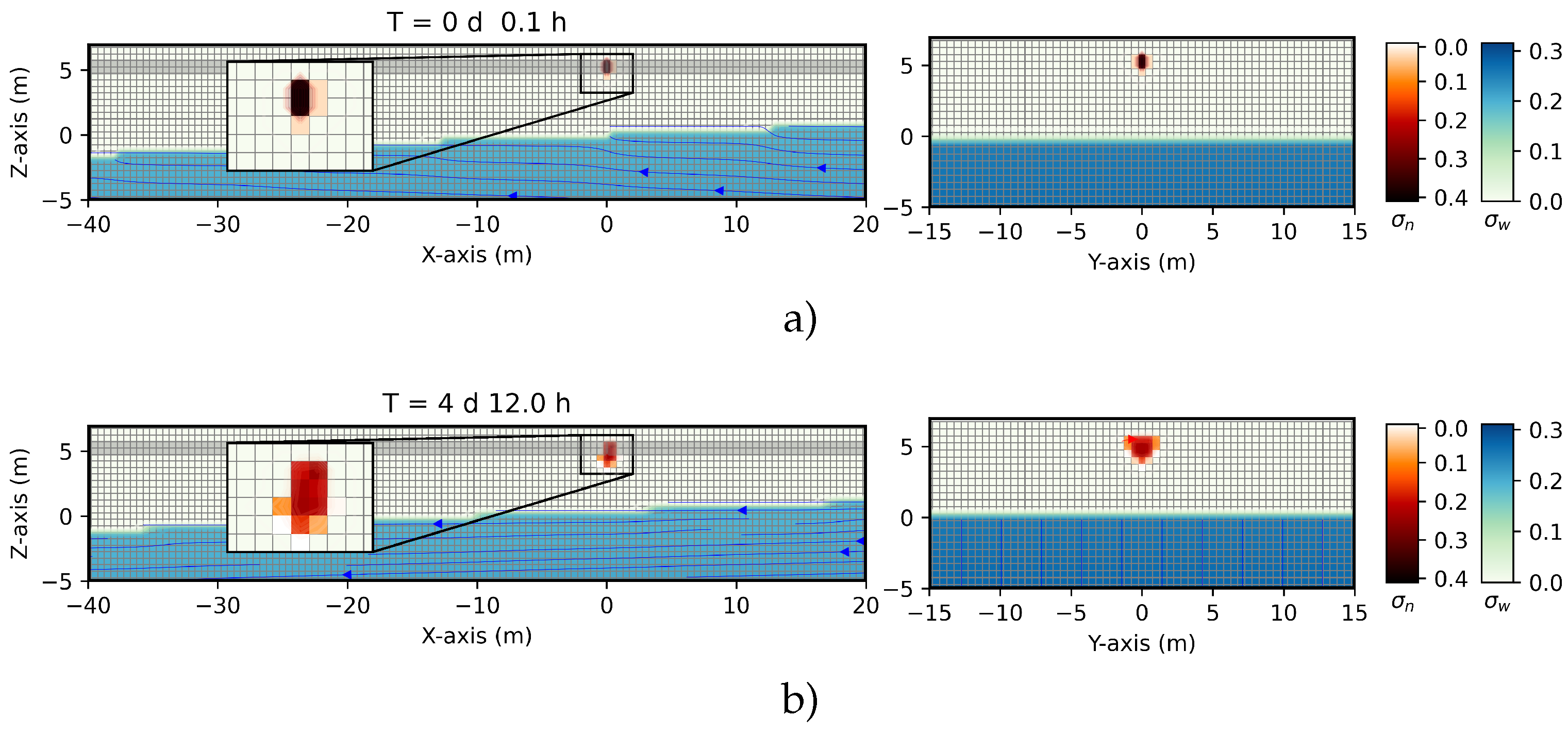
Figure 17.
3D transient numerical simulation results on the saturation contours of three immiscible phases (water, crude oil, and air) vs. the position, at different times. The crude oil is released from the pipeline at in the unsaturated zone with . Porosity value at the atmosphere pressure . (a) ; (b) . The left-hand side shows the plane, and the right-hand side shows the plane. Zoomed inset on the plane. Color bars on the right stand for , and .
Figure 17.
3D transient numerical simulation results on the saturation contours of three immiscible phases (water, crude oil, and air) vs. the position, at different times. The crude oil is released from the pipeline at in the unsaturated zone with . Porosity value at the atmosphere pressure . (a) ; (b) . The left-hand side shows the plane, and the right-hand side shows the plane. Zoomed inset on the plane. Color bars on the right stand for , and .
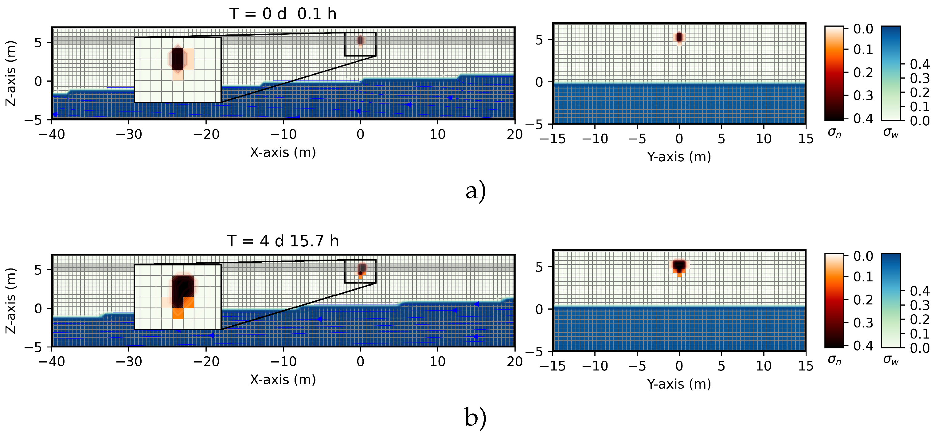
Figure 18.
3D transient numerical simulation results on the saturation contours of three immiscible phases (water, crude oil, and air) vs. the position, at different times. The crude oil is released from the pipeline at in the unsaturated zone with . Porosity value at the atmosphere pressure . (a) ; (b) . The left-hand side shows the plane, and the right-hand side shows the plane. Zoomed inset on the plane. Color bars on the right stand for , and .
Figure 18.
3D transient numerical simulation results on the saturation contours of three immiscible phases (water, crude oil, and air) vs. the position, at different times. The crude oil is released from the pipeline at in the unsaturated zone with . Porosity value at the atmosphere pressure . (a) ; (b) . The left-hand side shows the plane, and the right-hand side shows the plane. Zoomed inset on the plane. Color bars on the right stand for , and .
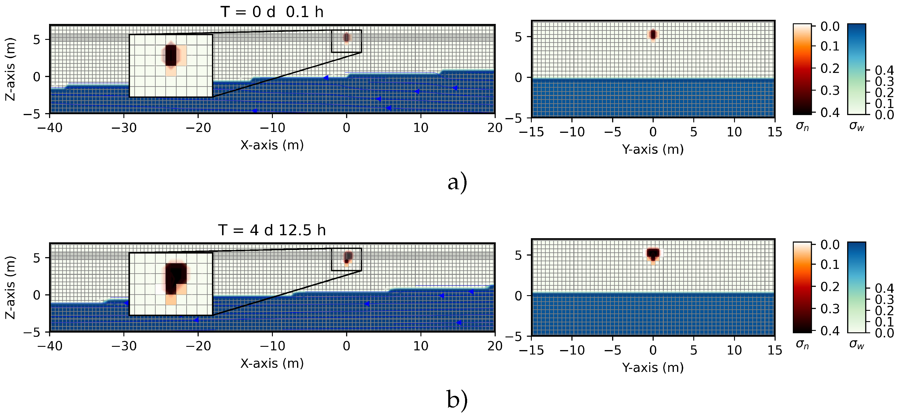
Figure 19.
3D transient numerical simulation results on the saturation contours of three immiscible phases (water, crude oil, and air) vs. the position, at different times. The crude oil is released from the pipeline at in the unsaturated zone with . Porosity value at the atmosphere pressure . (a) ; (b) . The left-hand side shows the plane, and the right-hand side shows the plane. Zoomed inset on the plane. Color bars on the right stand for , and .
Figure 19.
3D transient numerical simulation results on the saturation contours of three immiscible phases (water, crude oil, and air) vs. the position, at different times. The crude oil is released from the pipeline at in the unsaturated zone with . Porosity value at the atmosphere pressure . (a) ; (b) . The left-hand side shows the plane, and the right-hand side shows the plane. Zoomed inset on the plane. Color bars on the right stand for , and .
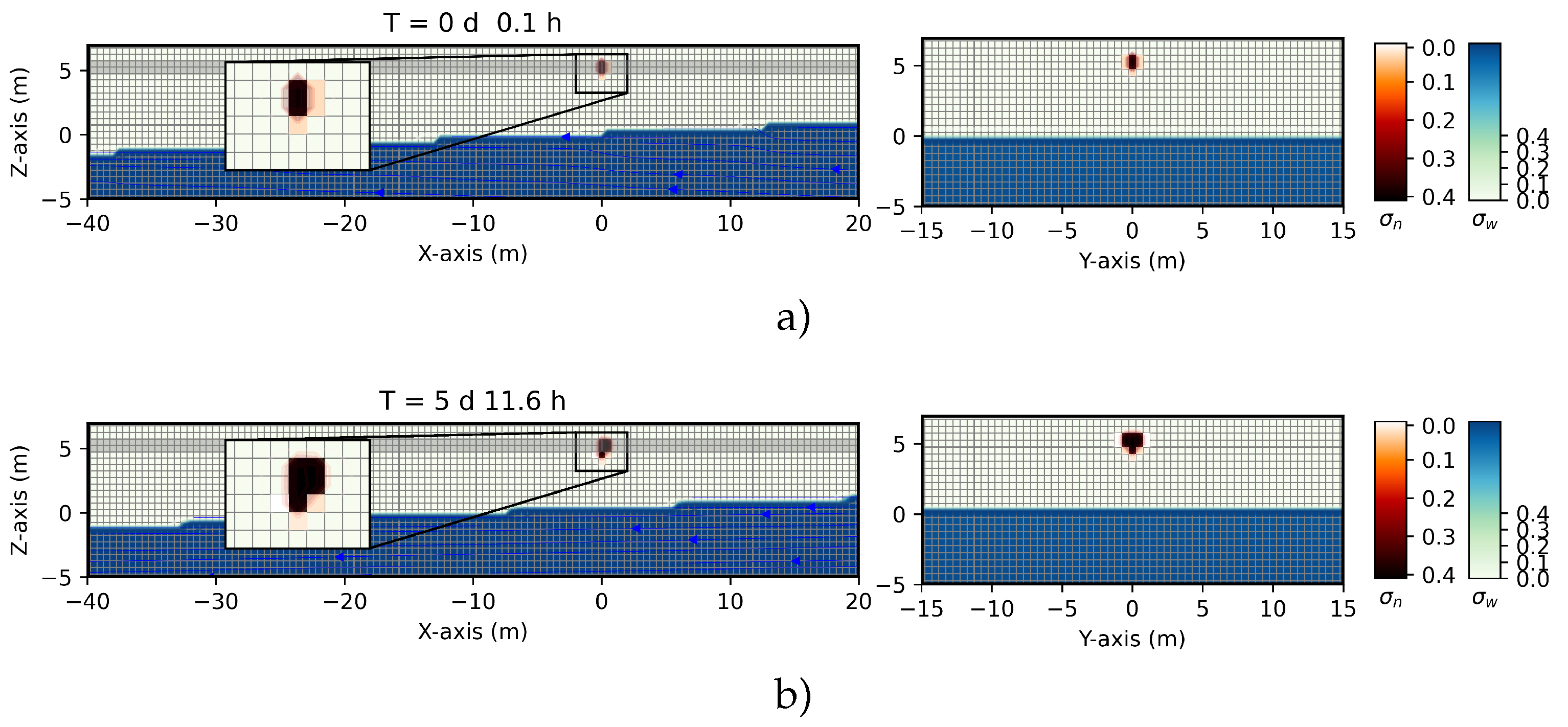
Figure 20.
Elevation vs. crude oil mass spilled at for and porosities values , and different times.
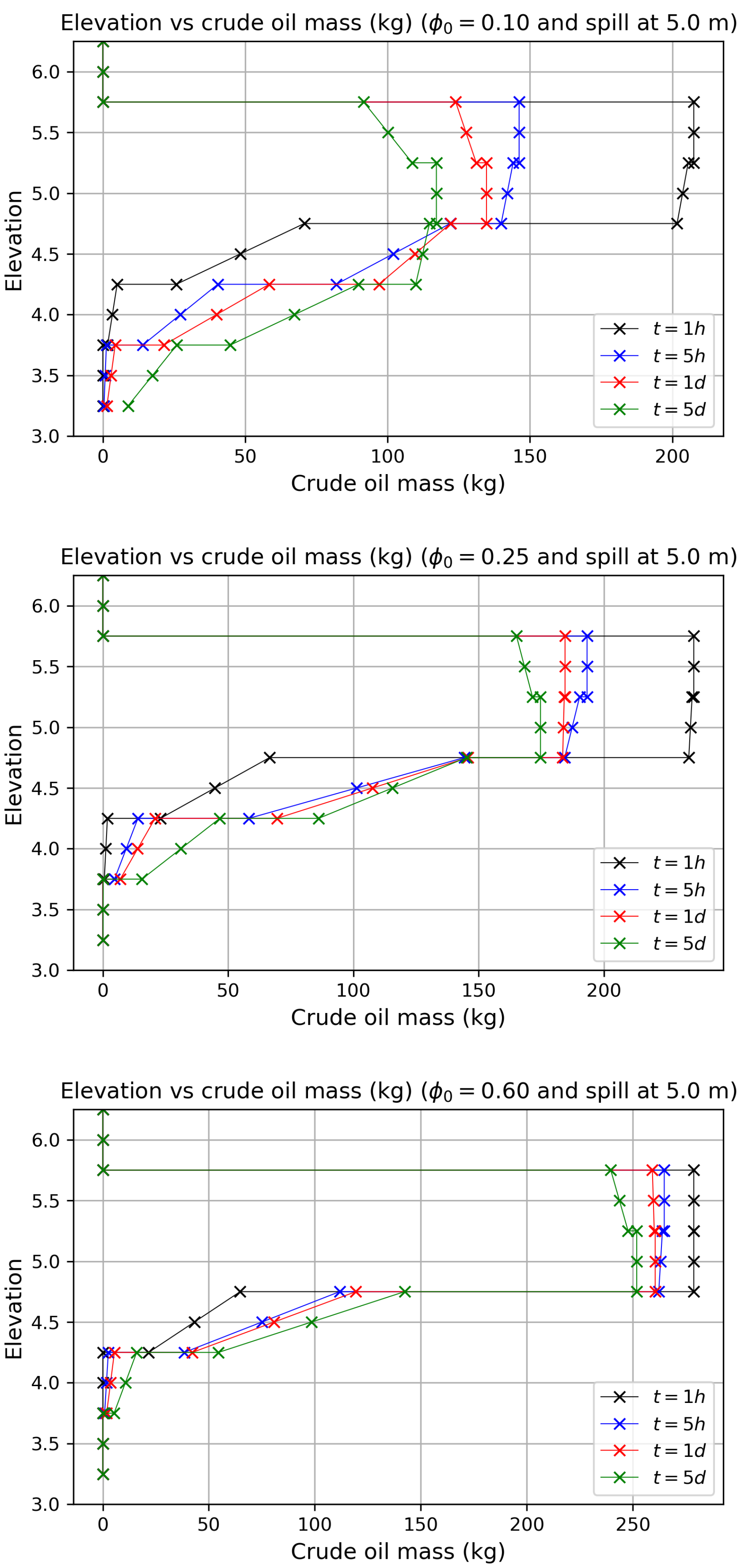
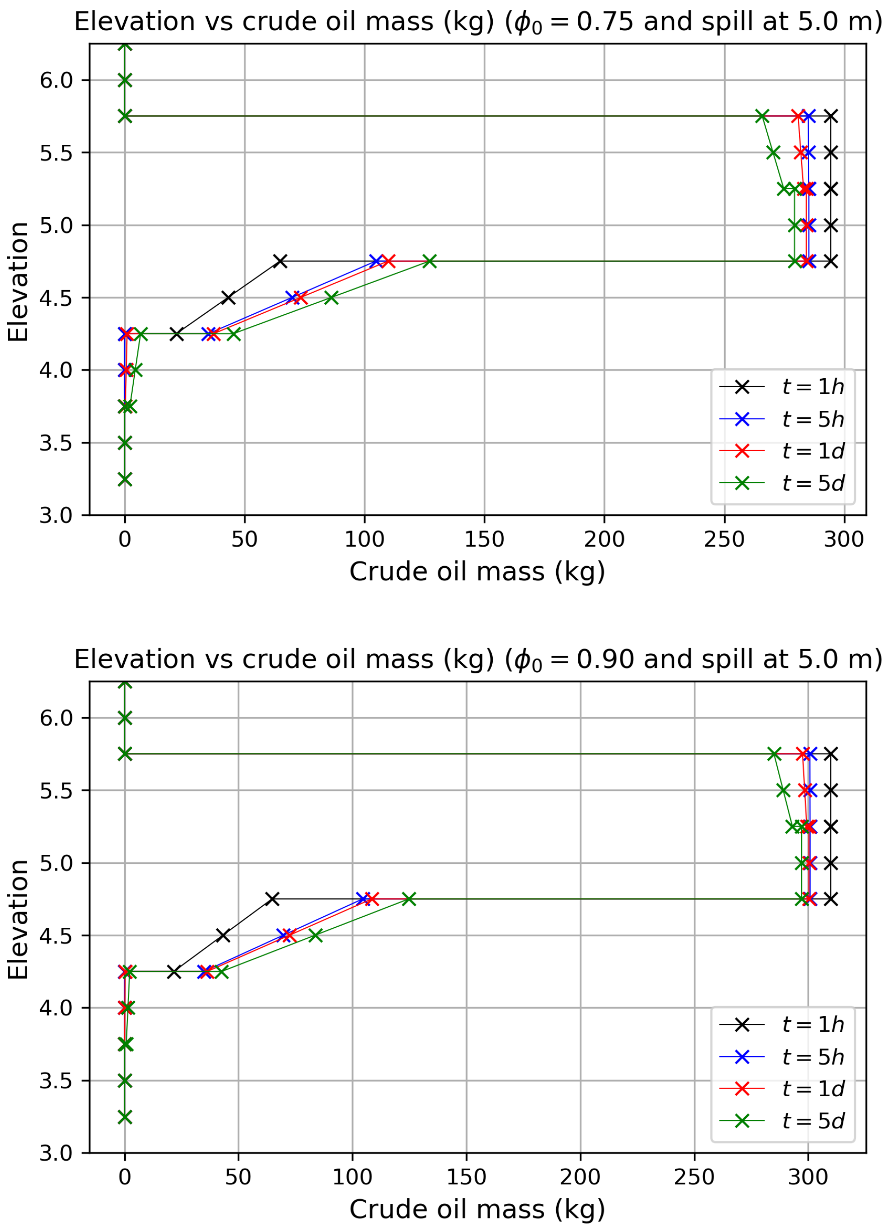
Figure 21.
Elevation vs. crude oil mass spilled at with , different porosity values , and different times:
Figure 21.
Elevation vs. crude oil mass spilled at with , different porosity values , and different times:
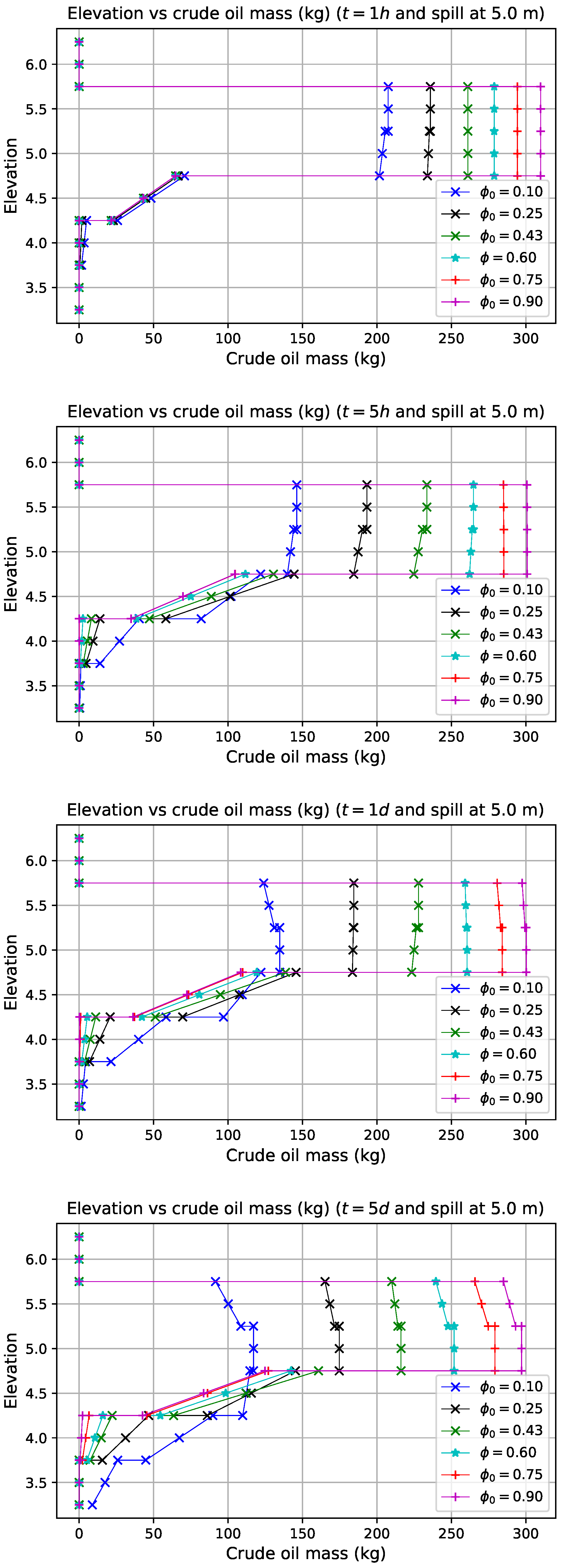
Figure 22.
Grid refinement scheme for the case of the crude oil spilled at and water saturation , and different times. (a) Spatial resolution of (b) Spatial resolution of (c) Spatial resolution of (d) Spatial resolution of (e) Spatial resolution of (f) Spatial resolution of .
Figure 22.
Grid refinement scheme for the case of the crude oil spilled at and water saturation , and different times. (a) Spatial resolution of (b) Spatial resolution of (c) Spatial resolution of (d) Spatial resolution of (e) Spatial resolution of (f) Spatial resolution of .
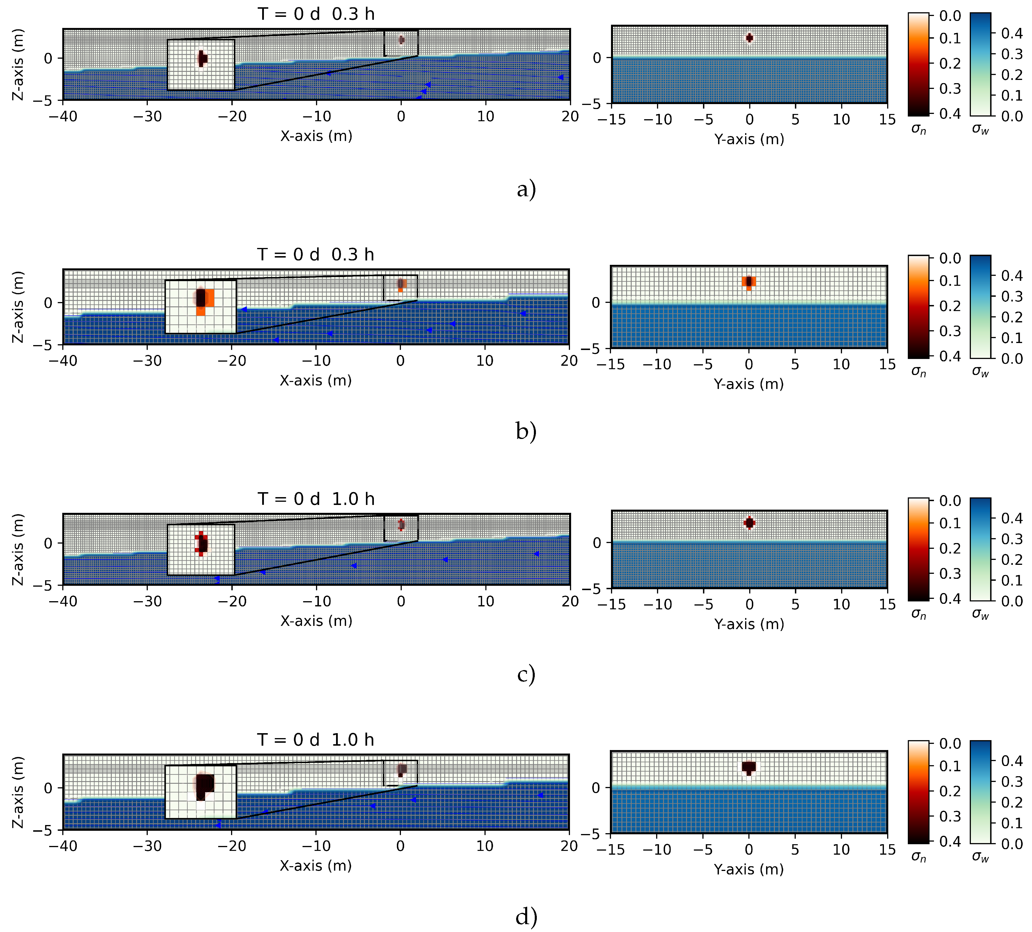
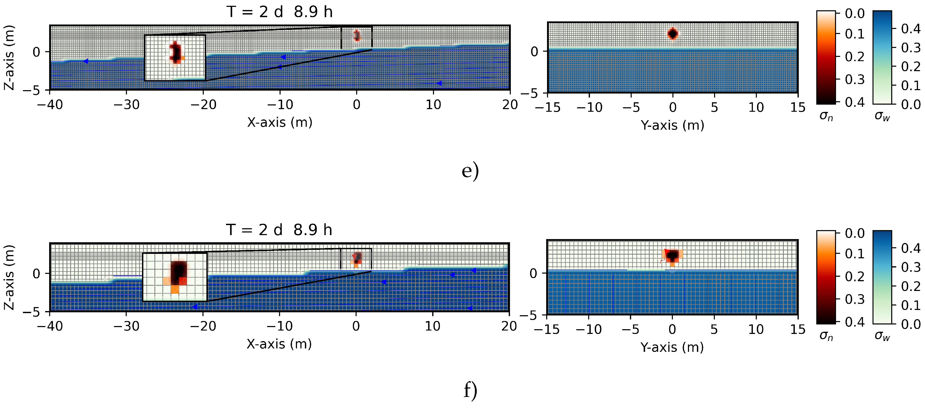

Table 1.
Crude oil features and hydrogeological parameters values used in the numerical simulations.
Table 1.
Crude oil features and hydrogeological parameters values used in the numerical simulations.
| Parameter | Definition | Value |
|---|---|---|
| Crude oil density | ||
| Crude oil dynamics viscosity | ||
| Water density | ||
| Water dynamics viscosity | ||
| Air density | ||
| Air dynamics viscosity | ||
| Superficial tension air-water | ||
| Superficial tension nonaqueous-water | ||
| Capillary pressure nonaqueous-water at zero saturation | ||
| Capillary pressure air-nonaqueous at zero saturation | ||
| Irreducible wetting phase saturation | 0.045 | |
| Absolute permeability | k | |
| Absolute permeability (bottom base and pipeline) | ||
| Porosity | 0.43 | |
| Rock compressibility | ||
| van Genuchten parameters |
Table 2.
Elevation of the crude oil spilled at the initial position , water saturation , and different times. The data are the one used in Figure 1.
Table 2.
Elevation of the crude oil spilled at the initial position , water saturation , and different times. The data are the one used in Figure 1.
| Water saturation | z elevation (m.a.s.l.) | crude oil mass per cell (kg) | Trapped contaminant in % |
|---|---|---|---|
| , hours | 0.0000 | 0.00 | |
| 261.0363 | 46.18 | ||
| 261.0449 | 46.18 | ||
| 43.2048 | 7.64 | ||
| 0.0060 | 0.00 | ||
| 0.0000 | 0.00 | ||
| , hours | 0.0000 | 0.00 | |
| 233.5149 | 42.04 | ||
| 227.6485 | 40.98 | ||
| 88.8148 | 15.99 | ||
| 5.5122 | 0.99 | ||
| 0.0000 | 0.00 | ||
| 0.0000 | 0.00 | ||
| , days | 0.0000 | 0.00 | |
| 212.0039 | 38.19 | ||
| 216.1497 | 38.94 | ||
| 112.1497 | 20.20 | ||
| 14.8048 | 2.67 | ||
| 0.0006 | 0.00 | ||
| 0.0000 | 0.00 | ||
| , days | 0.0000 | 0.00 | |
| 199.8475 | 36.00 | ||
| 208.0021 | 37.47 | ||
| 125.2007 | 22.55 | ||
| 22.0614 | 3.97 | ||
| 0.0088 | 0.00 | ||
| 0.0000 | 0.00 | ||
| , days | 0.0000 | 0.00 | |
| 191.3546 | 34.47 | ||
| 201.5328 | 36.30 | ||
| 133.3540 | 24.02 | ||
| 28.7539 | 5.18 | ||
| 0.1252 | 0.02 | ||
| 0.0000 | 0.00 | ||
| , days | 0.0000 | 0.00 | |
| 174.5964 | 31.45 | ||
| 186.2088 | 33.54 | ||
| 140.2680 | 25.27 | ||
| 49.5967 | 8.93 | ||
| 4.4506 | 0.80 | ||
| 0.0000 | 0.00 |
Table 3.
Elevation of the crude oil spilled at the initial position , water saturation , and different times. The data are the one used in Figure 2.
Table 3.
Elevation of the crude oil spilled at the initial position , water saturation , and different times. The data are the one used in Figure 2.
| Water saturation | z elevation (m.a.s.l.) | crude oil mass (kg) | Trapped contaminant in % |
|---|---|---|---|
| , hours | 0.0000 | 0.00 | |
| 260.8119 | 46.17 | ||
| 260.7718 | 46.16 | ||
| 43.2592 | 7.66 | ||
| 0.0581 | 0.01 | ||
| 0.0000 | 0.00 | ||
| 0.0000 | 0.00 | ||
| , hours | 0.0000 | 0.00 | |
| 229.7451 | 41.71 | ||
| 223.0453 | 40.49 | ||
| 91.7601 | 16.66 | ||
| 6.2896 | 1.14 | ||
| 0.0000 | 0.00 | ||
| 0.0000 | 0.00 | ||
| , days | 0.0000 | 0.00 | |
| 207.3996 | 37.68 | ||
| 212.5097 | 38.61 | ||
| 114.9301 | 20.88 | ||
| 15.5305 | 2.82 | ||
| 0.0072 | 0.00 | ||
| 0.0000 | 0.00 | ||
| , days | 0.0000 | 0.00 | |
| 194.3445 | 35.31 | ||
| 204.9642 | 37.24 | ||
| 127.1667 | 23.11 | ||
| 23.8446 | 4.33 | ||
| 0.0571 | 0.01 | ||
| 0.0000 | 0.00 | ||
| , days | 0.0000 | 0.00 | |
| 184.9861 | 33.61 | ||
| 198.5532 | 36.08 | ||
| 133.6930 | 24.29 | ||
| 32.7165 | 5.94 | ||
| 0.4283 | 0.08 | ||
| 0.0000 | 0.00 | ||
| , days | 0.0000 | 0.00 | |
| 177.7485 | 32.30 | ||
| 192.8687 | 35.04 | ||
| 136.3291 | 24.77 | ||
| 41.8632 | 7.61 | ||
| 1.5675 | 0.28 | ||
| 0.0000 | 0.00 |
Table 4.
Elevation of the crude oil spilled at the initial position , water saturation , and different times. The data are the one used in Figure 3.
Table 4.
Elevation of the crude oil spilled at the initial position , water saturation , and different times. The data are the one used in Figure 3.
| Water saturation | z elevation (m.a.s.l.) | crude oil mass (kg) | Trapped contaminant in % |
|---|---|---|---|
| , hours | 0.0000 | 0.00 | |
| 259.8364 | 46.14 | ||
| 259.6224 | 46.10 | ||
| 43.4674 | 7.72 | ||
| 0.2147 | 0.04 | ||
| 0.0000 | 0.00 | ||
| 0.0000 | 0.00 | ||
| , hours | 0.0000 | 0.00 | |
| 228.2995 | 41.63 | ||
| 221.7737 | 40.44 | ||
| 92.2273 | 16.82 | ||
| 6.0570 | 1.10 | ||
| 0.0001 | 0.00 | ||
| 0.0000 | 0.00 | ||
| , days | 0.0000 | 0.00 | |
| 199.1359 | 36.34 | ||
| 207.8144 | 37.93 | ||
| 123.9860 | 22.63 | ||
| 16.9984 | 3.10 | ||
| 0.0101 | 0.00 | ||
| 0.0000 | 0.00 | ||
| , days | 0.0000 | 0.00 | |
| 183.4905 | 33.49 | ||
| 197.2307 | 35.99 | ||
| 134.3200 | 24.51 | ||
| 32.5130 | 5.93 | ||
| 0.3907 | 0.07 | ||
| 0.0000 | 0.00 | ||
| , days | 0.0000 | 0.00 | |
| 173.2159 | 31.61 | ||
| 189.4214 | 34.57 | ||
| 136.6821 | 24.94 | ||
| 46.0553 | 8.41 | ||
| 2.5702 | 0.47 | ||
| 0.0000 | 0.00 | ||
| , days | 0.0000 | 0.00 | |
| 165.5615 | 30.22 | ||
| 182.4540 | 33.30 | ||
| 136.7272 | 24.95 | ||
| 56.9090 | 10.39 | ||
| 6.2931 | 1.15 | ||
| 0.0000 | 0.00 |
Table 5.
Elevation of the crude oil spilled at the initial position , water saturation , and different times. The data are the one used in Figure 4.
Table 5.
Elevation of the crude oil spilled at the initial position , water saturation , and different times. The data are the one used in Figure 4.
| Water saturation | z elevation (m.a.s.l.) | crude oil mass (kg) | Trapped contaminant in % |
|---|---|---|---|
| , hours | 0.0000 | 0.00 | |
| 259.0968 | 46.11 | ||
| 258.8111 | 46.06 | ||
| 43.6874 | 7.78 | ||
| 0.2662 | 0.05 | ||
| 0.0000 | 0.00 | ||
| 0.0000 | 0.00 | ||
| , hours | 0.0000 | 0.00 | |
| 227.7831 | 41.61 | ||
| 221.4593 | 40.46 | ||
| 92.1169 | 16.83 | ||
| 6.0144 | 1.10 | ||
| 0.0001 | 0.00 | ||
| 0.0000 | 0.00 | ||
| , days | 0.0000 | 0.00 | |
| 196.5772 | 35.94 | ||
| 203.2730 | 37.16 | ||
| 126.6544 | 23.16 | ||
| 20.4573 | 3.74 | ||
| 0.0034 | 0.00 | ||
| 0.0000 | 0.00 | ||
| , days | 0.0000 | 0.00 | |
| 180.6038 | 33.02 | ||
| 193.6267 | 35.40 | ||
| 133.5167 | 24.41 | ||
| 39.2148 | 7.17 | ||
| 0.0034 | 0.00 | ||
| 0.0000 | 0.00 | ||
| , days | 0.0000 | 0.00 | |
| 169.8303 | 31.05 | ||
| 185.3336 | 33.88 | ||
| 135.2435 | 24.73 | ||
| 56.5546 | 10.34 | ||
| 0.0034 | 0.00 | ||
| 0.0000 | 0.00 | ||
| , days | 0.0000 | 0.00 | |
| 164.7161 | 30.11 | ||
| 180.8585 | 33.07 | ||
| 135.4080 | 24.76 | ||
| 65.9773 | 12.06 | ||
| 0.0054 | 0.00 | ||
| 0.0000 | 0.00 |
Table 6.
Elevation of the crude oil spilled at the initial position , water saturation , and different times. The data are the one used in Figure 5.
Table 6.
Elevation of the crude oil spilled at the initial position , water saturation , and different times. The data are the one used in Figure 5.
| Water saturation | z elevation (m.a.s.l.) | crude oil mass (kg) | Trapped contaminant in % |
|---|---|---|---|
| , hours | 0.0000 | 0.00 | |
| 258.8941 | 46.10 | ||
| 258.6339 | 46.06 | ||
| 43.7718 | 7.79 | ||
| 0.2573 | 0.05 | ||
| 0.0000 | 0.00 | ||
| 0.0000 | 0.00 | ||
| , hours | 0.0000 | 0.00 | |
| 227.7831 | 41.61 | ||
| 221.4593 | 40.46 | ||
| 92.1169 | 16.83 | ||
| 6.0144 | 1.10 | ||
| 0.0001 | 0.00 | ||
| 0.0000 | 0.00 | ||
| , days | 0.0000 | 0.00 | |
| 200.9746 | 36.79 | ||
| 222.3319 | 40.70 | ||
| 115.1350 | 21.08 | ||
| 7.8671 | 1.44 | ||
| 0.0003 | 0.00 | ||
| 0.0000 | 0.00 | ||
| , days | 0.0000 | 0.00 | |
| 198.8378 | 36.40 | ||
| 222.2577 | 40.68 | ||
| 117.0380 | 21.42 | ||
| 8.1751 | 1.50 | ||
| 0.0003 | 0.00 | ||
| 0.0000 | 0.00 | ||
| , days | 0.0000 | 0.00 | |
| 169.8303 | 31.05 | ||
| 185.3336 | 33.88 | ||
| 135.2435 | 24.73 | ||
| 56.5546 | 10.34 | ||
| 0.0034 | 0.00 | ||
| 0.0000 | 0.00 |
Table 7.
Elevation of the crude oil spilled at the initial position , water saturation , and different times. The data are the one used in Figure 8.
Table 7.
Elevation of the crude oil spilled at the initial position , water saturation , and different times. The data are the one used in Figure 8.
| Water saturation | z elevation (m.a.s.l.) | crude oil mass per cell (kg) | Trapped contaminant in % |
|---|---|---|---|
| , hours | 0.0000 | 0.00 | |
| 261.0363 | 46.18 | ||
| 261.0449 | 46.18 | ||
| 43.2048 | 7.64 | ||
| 0.0060 | 0.00 | ||
| 0.0000 | 0.00 | ||
| , hours | 0.0000 | 0.00 | |
| 233.5149 | 42.04 | ||
| 227.6485 | 40.98 | ||
| 88.8148 | 15.99 | ||
| 5.5122 | 0.99 | ||
| 0.0000 | 0.00 | ||
| , days | 0.0000 | 0.00 | |
| 227.9310 | 41.06 | ||
| 224.8579 | 40.51 | ||
| 94.88008 | 17.09 | ||
| 7.4509 | 1.34 | ||
| 0.0000 | 0.00 | ||
| , days | 0.0000 | 0.00 | |
| 212.0039 | 38.19 | ||
| 216.1616 | 38.94 | ||
| 112.1497 | 20.20 | ||
| 14.8048 | 2.67 | ||
| 0.0006 | 0.00 | ||
| , days | 0.0000 | 0.00 | |
| 199.8475 | 36.00 | ||
| 208.0021 | 37.47 | ||
| 125.2007 | 22.55 | ||
| 22.0614 | 3.97 | ||
| 0.0088 | 0.00 | ||
| , days | 0.0000 | 0.00 | |
| 191.3546 | 34.47 | ||
| 201.5328 | 36.30 | ||
| 133.3540 | 24.02 | ||
| 28.7539 | 5.18 | ||
| 0.1252 | 0.02 |
Table 8.
Elevation of the crude oil spilled at , water saturation , and different times. The data are the one used in Figure 9.
Table 8.
Elevation of the crude oil spilled at , water saturation , and different times. The data are the one used in Figure 9.
| Water saturation | z elevation (m.a.s.l.) | crude oil mass per cell (kg) | Trapped contaminant in % |
|---|---|---|---|
| , hours | 0.0000 | 0.00 | |
| 260.8119 | 46.17 | ||
| 260.7718 | 46.16 | ||
| 43.2592 | 7.66 | ||
| 0.0581 | 0.01 | ||
| 0.0000 | 0.00 | ||
| , hours | 0.0000 | 0.00 | |
| 229.7451 | 41.71 | ||
| 233.0453 | 40.49 | ||
| 91.7601 | 16.66 | ||
| 6.2896 | 1.14 | ||
| 0.0000 | 0.00 | ||
| , days | 0.0000 | 0.00 | |
| 223.9634 | 40.69 | ||
| 220.3788 | 40.04 | ||
| 97.8541 | 17.78 | ||
| 8.1804 | 1.49 | ||
| 0.0003 | 0.00 | ||
| , days | 0.0000 | 0.00 | |
| 207.3996 | 37.68 | ||
| 212.5098 | 38.61 | ||
| 114.9306 | 20.88 | ||
| 15.5300 | 2.82 | ||
| 0.0071 | 0.00 |
Table 9.
Elevation of the crude oil spilled at the initial position , water saturation , and different times. The data are the one used in Figure 10.
Table 9.
Elevation of the crude oil spilled at the initial position , water saturation , and different times. The data are the one used in Figure 10.
| Water saturation | z elevation (m.a.s.l.) | crude oil mass per cell (kg) | Trapped contaminant in % |
|---|---|---|---|
| , hours | 0.0000 | 0.00 | |
| 259.8364 | 46.14 | ||
| 259.6224 | 46.10 | ||
| 43.4674 | 7.72 | ||
| 0.2147 | 0.04 | ||
| 0.0000 | 0.00 | ||
| , hours | 0.0000 | 0.00 | |
| 228.2995 | 41.63 | ||
| 221.7737 | 40.44 | ||
| 92.2273 | 16.82 | ||
| 6.0570 | 1.10 | ||
| 0.0001 | 0.00 | ||
| , days | 0.0000 | 0.00 | |
| 221.1071 | 40.35 | ||
| 220.3577 | 40.22 | ||
| 98.6146 | 18.00 | ||
| 7.8647 | 1.44 | ||
| 0.0006 | 0.00 | ||
| , days | 0.0000 | 0.00 | |
| 199.1366 | 36.34 | ||
| 207.8110 | 37.93 | ||
| 124.0196 | 22.63 | ||
| 16.9677 | 3.10 | ||
| 0.0098 | 0.00 |
Table 10.
Elevation of the crude oil spilled at the initial position , water saturation , and different times. The data are the one used in Figure 11.
Table 10.
Elevation of the crude oil spilled at the initial position , water saturation , and different times. The data are the one used in Figure 11.
| Water saturation | z elevation (m.a.s.l.) | crude oil mass per cell (kg) | Trapped contaminant in % |
|---|---|---|---|
| , hours | 0.0000 | 0.00 | |
| 259.0968 | 46.11 | ||
| 258.8111 | 46.06 | ||
| 43.6874 | 7.78 | ||
| 0.2662 | 0.05 | ||
| 0.0000 | 0.00 | ||
| , hours | 0.0000 | 0.00 | |
| 227.7831 | 41.61 | ||
| 221.4593 | 40.46 | ||
| 92.1169 | 16.83 | ||
| 6.0144 | 1.10 | ||
| 0.0001 | 0.00 | ||
| , days | 0.0000 | 0.00 | |
| 218.3717 | 39.92 | ||
| 221.3647 | 40.47 | ||
| 99.3309 | 18.16 | ||
| 7.8973 | 1.44 | ||
| 0.0007 | 0.00 | ||
| , days | 0.0000 | 0.00 | |
| 196.5739 | 35.94 | ||
| 203.2794 | 37.16 | ||
| 126.6577 | 23.16 | ||
| 20.4389 | 3.74 | ||
| 0.0154 | 0.00 |
Table 11.
Elevation of the crude oil spilled at the initial position , water saturation , and different times. The data are the one used in Figure 12.
Table 11.
Elevation of the crude oil spilled at the initial position , water saturation , and different times. The data are the one used in Figure 12.
| Water saturation | z elevation (m.a.s.l.) | crude oil mass per cell (kg) | Trapped contaminant in % |
|---|---|---|---|
| , hours | 0.0000 | 0.00 | |
| 258.8941 | 46.10 | ||
| 258.6339 | 46.06 | ||
| 43.7718 | 7.79 | ||
| 0.2573 | 0.05 | ||
| 0.0000 | 0.00 | ||
| , hours | 0.0000 | 0.00 | |
| 227.6235 | 41.47 | ||
| 221.3969 | 41.60 | ||
| 92.0988 | 16.83 | ||
| 6.0069 | 1.10 | ||
| 0.0001 | 0.00 | ||
| , days | 0.0000 | 0.00 | |
| 216.8538 | 39.68 | ||
| 221.9299 | 40.61 | ||
| 99.7383 | 18.25 | ||
| 7.9244 | 1.45 | ||
| 0.0007 | 0.00 | ||
| , days | 0.0000 | 0.00 | |
| 191.6971 | 35.09 | ||
| 201.4679 | 36.88 | ||
| 130.8024 | 23.94 | ||
| 22.3268 | 4.09 | ||
| 0.0239 | 0.00 |
Table 12.
Elevation of the crude oil spilled at the initial position , water saturation , porosity , and different times. The data are the one used in Figure 12.
Table 12.
Elevation of the crude oil spilled at the initial position , water saturation , porosity , and different times. The data are the one used in Figure 12.
| Porosity values | z elevation (m.a.s.l.) | crude oil mass per cell (kg) | Trapped contaminant in % |
|---|---|---|---|
| , hours | 0.0000 | 0.00 | |
| 207.5226 | 44.84 | ||
| 203.6071 | 44.00 | ||
| 48.2827 | 10.43 | ||
| 3.3613 | 0.73 | ||
| 0.0000 | 0.00 | ||
| 0.0000 | 0.00 | ||
| , hours | 0.0000 | 0.00 | |
| 146.1899 | 34.96 | ||
| 141.9819 | 33.95 | ||
| 101.9783 | 24.39 | ||
| 27.1917 | 6.50 | ||
| 0.8414 | 0.20 | ||
| 0.0000 | 0.00 | ||
| , days | 0.0000 | 0.00 | |
| 127.5240 | 30.76 | ||
| 134.7329 | 32.49 | ||
| 109.5543 | 26.42 | ||
| 39.9153 | 9.63 | ||
| 2.9017 | 0.70 | ||
| 0.0000 | 0.00 | ||
| , days | 0.0000 | 0.00 | |
| 100.1320 | 24.15 | ||
| 117.1464 | 28.25 | ||
| 112.3013 | 27.08 | ||
| 67.2712 | 16.22 | ||
| 17.4334 | 4.200 | ||
| 0.3441 | 0.08 |
Table 13.
Elevation of the crude oil spilled at the initial position , water saturation , porosity , and different times. The data are the one used in Figure 12.
Table 13.
Elevation of the crude oil spilled at the initial position , water saturation , porosity , and different times. The data are the one used in Figure 12.
| Porosity values | z elevation (m.a.s.l.) | crude oil mass per cell (kg) | Trapped contaminant in % |
|---|---|---|---|
| , hours | 0.0000 | 0.00 | |
| 235.8787 | 45.68 | ||
| 234.5438 | 45.42 | ||
| 44.7818 | 8.67 | ||
| 1.2240 | 0.24 | ||
| 0.0000 | 0.00 | ||
| 0.0000 | 0.00 | ||
| , hours | 0.0000 | 0.00 | |
| 193.2849 | 39.34 | ||
| 187.3403 | 38.13 | ||
| 101.3156 | 20.62 | ||
| 9.3446 | 1.90 | ||
| 0.0000 | 0.00 | ||
| 0.0000 | 0.00 | ||
| , days | 0.0000 | 0.00 | |
| 184.4936 | 37.66 | ||
| 183.8570 | 37.53 | ||
| 107.6380 | 21.97 | ||
| 13.9150 | 2.84 | ||
| 0.0010 | 0.00 | ||
| 0.0000 | 0.00 | ||
| , days | 0.0000 | 0.00 | |
| 168.3081 | 34.36 | ||
| 174.6942 | 35.66 | ||
| 115.6516 | 23.61 | ||
| 31.1579 | 6.36 | ||
| 0.0926 | 0.00 | ||
| 0.0000 | 0.00 |
Table 14.
Elevation of the crude oil spilled at the initial position , water saturation , porosity , and different times. The data are the one used in Figure 12.
Table 14.
Elevation of the crude oil spilled at the initial position , water saturation , porosity , and different times. The data are the one used in Figure 12.
| Porosity values | z elevation (m.a.s.l.) | crude oil mass per cell (kg) | Trapped contaminant in % |
|---|---|---|---|
| , hours | 0.0000 | 0.00 | |
| 278.7295 | 46.40 | ||
| 278.7314 | 46.41 | ||
| 43.1875 | 7.19 | ||
| 0.0004 | 0.00 | ||
| 0.0000 | 0.00 | ||
| 0.0000 | 0.00 | ||
| , hours | 0.0000 | 0.00 | |
| 264.8098 | 43.79 | ||
| 263.0759 | 43.51 | ||
| 75.0377 | 12.41 | ||
| 1.7378 | 0.29 | ||
| 0.0000 | 0.00 | ||
| 0.0000 | 0.00 | ||
| , days | 0.0000 | 0.00 | |
| 259.6473 | 42.95 | ||
| 260.5327 | 43.09 | ||
| 80.7632 | 13.36 | ||
| 3.6410 | 0.60 | ||
| 0.0010 | 0.00 | ||
| 0.0000 | 0.00 | ||
| , days | 0.0000 | 0.00 | |
| 243.6698 | 40.30 | ||
| 251.8302 | 41.65 | ||
| 98.4418 | 16.28 | ||
| 10.6424 | 1.76 | ||
| 0.0000 | 0.00 | ||
| 0.0000 | 0.00 |
Table 15.
Elevation of the crude oil spilled at the initial position , water saturation , porosity , and different times. The data are the one used in Figure 12.
Table 15.
Elevation of the crude oil spilled at the initial position , water saturation , porosity , and different times. The data are the one used in Figure 12.
| Porosity values | z elevation (m.a.s.l.) | crude oil mass per cell (kg) | Trapped contaminant in % |
|---|---|---|---|
| , hours | 0.0000 | 0.00 | |
| 294.3289 | 46.58 | ||
| 294.3296 | 46.58 | ||
| 43.1842 | 6.83 | ||
| 0.0000 | 0.00 | ||
| 0.0000 | 0.00 | ||
| 0.0000 | 0.00 | ||
| , hours | 0.0000 | 0.00 | |
| 285.0378 | 44.53 | ||
| 285.1806 | 44.55 | ||
| 69.8498 | 10.91 | ||
| 0.0866 | 0.01 | ||
| 0.0000 | 0.00 | ||
| 0.0000 | 0.00 | ||
| , days | 0.0000 | 0.00 | |
| 281.8594 | 44.03 | ||
| 284.1341 | 44.39 | ||
| 73.4374 | 11.47 | ||
| 0.7240 | 0.11 | ||
| 0.0000 | 0.00 | ||
| 0.0000 | 0.00 | ||
| , days | 0.0000 | 0.00 | |
| 270.2436 | 42.22 | ||
| 279.2238 | 43.62 | ||
| 86.2152 | 13.47 | ||
| 4.4723 | 0.70 | ||
| 0.0000 | 0.00 | ||
| 0.0000 | 0.00 |
Table 16.
Elevation of the crude oil spilled at the initial position , water saturation , porosity , and different times. The data are the one used in Figure 12.
Table 16.
Elevation of the crude oil spilled at the initial position , water saturation , porosity , and different times. The data are the one used in Figure 12.
| Porosity values | z elevation (m.a.s.l.) | crude oil mass per cell (kg) | Trapped contaminant in % |
|---|---|---|---|
| , hours | 0.0000 | 0.00 | |
| 309.9264 | 46.74 | ||
| 309.9267 | 46.74 | ||
| 43.1831 | 6.51 | ||
| 0.0000 | 0.00 | ||
| 0.0000 | 0.00 | ||
| 0.0000 | 0.00 | ||
| , hours | 0.0000 | 0.00 | |
| 300.7799 | 44.80 | ||
| 300.8593 | 44.81 | ||
| 69.6913 | 10.38 | ||
| 0.0203 | 0.00 | ||
| 0.0000 | 0.00 | ||
| 0.0000 | 0.00 | ||
| , days | 0.0000 | 0.00 | |
| 298.4708 | 44.46 | ||
| 300.3190 | 44.73 | ||
| 72.3847 | 10.78 | ||
| 0.1763 | 0.03 | ||
| 0.0000 | 0.00 | ||
| 0.0000 | 0.00 | ||
| , days | 0.0000 | 0.00 | |
| 289.0365 | 43.05 | ||
| 297.1403 | 44.26 | ||
| 83.6589 | 12.46 | ||
| 1.5153 | 0.23 | ||
| 0.0000 | 0.00 | ||
| 0.0000 | 0.00 |
Disclaimer/Publisher’s Note: The statements, opinions and data contained in all publications are solely those of the individual author(s) and contributor(s) and not of MDPI and/or the editor(s). MDPI and/or the editor(s) disclaim responsibility for any injury to people or property resulting from any ideas, methods, instructions or products referred to in the content. |
© 2026 by the authors. Licensee MDPI, Basel, Switzerland. This article is an open access article distributed under the terms and conditions of the Creative Commons Attribution (CC BY) license (http://creativecommons.org/licenses/by/4.0/).
Copyright: This open access article is published under a Creative Commons CC BY 4.0 license, which permit the free download, distribution, and reuse, provided that the author and preprint are cited in any reuse.


