

Submitted:
12 June 2026
Posted:
18 June 2026
You are already at the latest version
Abstract
The rapid expansion of artificial intelligence raises critical questions about its environmental implications in an increasingly globalized world. In this study, we explore the impact of Artificial Intelligence (AI) on environmental sustainability and its role in globalization, which bears significant implications for global sustainability in the digital era. We used the comprehensive evaluation index of the artificial intelligence index established by the Principal Component Analysis (PCA) method on a sample of 62 countries globally, from 2000 to 2022. Our study is based on the estimation of the Autoregressive Distributed Lag (ARDL) model, which distinguishes between short- and long-term dynamics. We noted that the overall level of global AI shows an upward trend. The research results show that AI has a positive and significant inhibitory effect on ecological footprints and greenhouse gas emissions in the long term. In addition, affected by globalization, the effects of AI on environmental sustainability show nonlinear characteristics. AI’s marginal effect on reducing environmental degradation increases. These findings emphasize the important role of AI in environmental governance and provide a new and comprehensive perspective for policymakers. Policymakers should prioritize AI R&D investment, promote cross-sectoral AI integration and strengthen international cooperation to maximize environmental benefits.
Keywords:
artificial intelligence
; greenhouse gas emissions
; ecological footprint of consumption
; globalization
; ARDL
; panel threshold model
; environmental sustainability
1. Introduction
The stability and sustainability of our climate are essential for humans to survive [1] and to reach sustainable development [2]. Nonetheless, the planet’s average temperature has risen by 1.5°C compared to pre-industrial levels [3], primarily due to anthropogenic greenhouse gas emissions [4]. This reality has led to widespread recognition of the need for transformative action to align development paradigms with climate mitigation principles [5,6,7,8].
Current environmental challenges, including overconsumption of natural resources, ecological degradation, and biodiversity loss [9] endanger the planet’s ecological balance [10]. The concept of the Ecological Footprint of Consumption (EFC), introduced by Wackernagel and Rees [11], provides a comprehensive assessment of environmental quality and reveals that 75% of countries are in ecological deficit [12], thus exacerbating ecological imbalances [13]. Artificial intelligence (AI) and globalization (GLB) play an increasingly significant role in this dynamic. Thanks to its ability to optimize renewable energy use and encourage energy-efficient choices [14,15], AI can contribute to reducing the EFC, despite its initial energy costs [16,17]. Globalization, on the other hand, has a dual impact on the environment, promoting both Economic Growth (EG) and ecological degradation [18,19]. Finally, Foreign direct investment (FDI) can either exacerbate pollution (pollution haven hypothesis) or improve environmental quality (pollution halo hypothesis) through green technologies [20]. These complex interactions require in-depth analysis in order to guide sustainable development policies. In light of the pressing issues surrounding global environmental concerns and greenhouse gas emissions, this study aims to address these pivotal issues:
Does AI influence environmental sustainability? Does AI affect environmental sustainability under the effect of globalization?
To investigate these issues, this work aims to empirically analyze the complex relationship between AI, environmental sustainability (ES) and globalization, based on a robust econometric approach applied to a panel of 62 high- and middle-income countries following the World Bank (WB) classification 2023 over the period 2000–2022. The influence of artificial intelligence on ES is studied by econometrically analyzing the relationships between the two indicators of environmental and artificial intelligence, while integrating relevant macroeconomic variables as well as control variables. This approach is based on the methodology of Wang et al [21], using data from the WB and the International Labour Organization (ILO).
The study first applies the principal composite analyses (PCA) method to measure comprehensive indices for artificial intelligence and institutional quality. Next, the short- and long-term relationships are estimated using the MG-ARDL, PMG-ARDL, and DFE-ARDL methods. In addition, a threshold model is applied to capture the potential nonlinear effects of artificial intelligence under different GLB intensities. They also shape strategies to fast-track digital transformation and create a greener and more sustainable future. Insights from the world’s largest economies can provide useful guidance for tackling environmental issues as well as other challenges in additional fields. Ultimately, this research encourages the use of AI as a way to drive automation, digital transformation and intelligent systems. It also enables resource demands reduction and environmental strain while promoting sustainable development. This approach guarantees the reliability of the results obtained and allows for a better understanding of the structural conditions under which artificial intelligence could effectively contribute to the global ecological transition.
Our study contributes to the literature in several ways. First, it draws on Ecological World System Theory (EWST) to analyze the short- and long-term effects of artificial intelligence (AI) on the environment and Pollution Haven or Helo Theory (PHHT) to assess the moderating role of globalization. Moreover, empirically, we use two complementary dependent variables: greenhouse gas (GHG) emissions and ecological footprint of consumption (EFC), which capture both the quality and quantity of environmental resources. This approach goes beyond studies limited to CO₂ and is in line with the most relevant sustainability indicators recently identified [22,23,24]. Finally, our models incorporate globalization to detect possible nonlinear effects, as well as FDI, ED, trade openness and the institutional quality index as control variables, reducing omitted variable bias. We also apply advanced estimation techniques: ARDL panel for the short- and long-term relationships of EWST theory, and threshold model to identify the level of globalization at which AI improves environmental performance of PHH theory. Figure 1 illustrates the conceptual framework of the artificial intelligence – environmental sustainability nexus and the moderation role of globalization. Figure 1 illustrates the conceptual framework of the artificial intelligence – environmental sustainability nexus and the moderation role of globalization of our study.
This study is structured into four sections. First, the "theoretical frameworks" section presents various theoretical perspectives. Next, the second section, "materials and methods", outlines the model specifications, data sources, and empirical methodologies. Then the third section presents the "results and discussion" of the findings. Finally, the "concluding" section offers recommendations based on our findings.
2. Theoretical Frameworks and Hypotheses
Due to global warming and climate change, the Pollution Haven or Helo Theory (PHHT) and Ecological World-Systems Theory (EWST) are considered two of the most significant issues in the literature. Furthermore, PHHT claims that some countries- especially developing countries that have lax environmental regulations, cheap labor force and abundant natural resources- gain comparative advantage in attracting multinational firms. In addition, developing countries´ governments support foreign investment inflows as a way to reduce the foreign trade deficit.
Nevertheless, it is argued that disparities between developed and developing countries – particularly in terms of labor costs, stringent environmental standards and availability of natural resources – can encourage multinational companies to relocate their investments to countries where environmental legislation is more flexible, less controlled or difficult to enforce as a way to cut costs and gain regulatory leeway. This strategy, often referred to as environmental dumping, enables them to circumvent the ecological constraints in force in their home countries, to the detriment of ES on a global scale. This means that an increase in FDI inflows may lead to a decrease in the host countries’ environmental quality. Finally, The EWST should take into account the regional distribution of the environmental impacts of digitalization, distinguishing between core regions that are economically developed, semi-peripheral regions that are emerging, and peripheral regions that remain less developed. One of the main arguments of EWST is that since core countries have been historically and still are dependent on exploiting the natural resources of peripheral countries, the latter bear the brunt of the environmental and social consequences [25].
In this context, we will present how environmental sustainability is influenced by multiple interconnected economical theories. The Ecological World Systems Theory (EWST) emphasizes global structural inequalities, with technologies like artificial intelligence offering both risks and opportunities for balancing environmental pressures. Meanwhile, we will present the pollution haven or halo hypotheses, how globalization can either worsen sustainability by shifting polluting industries to countries with weaker regulations or improve it by spreading greener practices and technologies. Together, these perspectives highlight that achieving sustainability requires managing the complex interplay between growth, technology, and globalization.
2.1. Theories of Digitalization and Environmental Sustainability
In this section, we provide an in-depth overview of the key theories that explore the connection between digitalization and environmental sustainability. Special attention is given to the role of hardware, ICT infrastructure, and software solutions in either improving or harming environmental quality, for example by increasing or decreasing Greenhouse Gas (GHG) emissions. The three theories discussed below highlight the important role of the digitalization product lifecycle, digitalization value chain (regional distribution of the environmental effects), and the use of smart devices. For instance, the production, use, and disposal of hardware devices (e.g., computers, servers, and networking equipment) contribute significantly to GHG emissions. It is well acknowledged that producing these hardware devices is highly energy-intensive and involves the extraction of raw materials with high carbon footprints. Likewise, the ICT infrastructure that enables digital systems- including data centers and data transmission equipment- requires a continuous power supply and energy-intensive cooling systems. Additionally, software products indirectly affect environmental quality through their development, distribution, and use. Together, these channels illustrate the various ways in which different components of digitalization can either improve or harm environmental conditions.
One relevant perspective, closely aligned with the work of Hilty et al. [26], is the Ecological World Systems Theory (EWST). Developed by Lennerfors et al. [25], this theory builds on earlier contributions by Hopkins and Wallerstein [27] and Hornborg [28,29]. Drawing from Hilty et al.'s [26] categorization of digitalization’s effects into first-, second-, and third-order impacts, EWST focuses on examining the unequal global distribution of environmental degradation driven by technological progress. It offers a framework for understanding how the environmental costs of digitalization are often disproportionately borne by certain regions or populations. From a practical standpoint, this framework proves valuable for assessing the environmental impact of digitalization through a life-cycle analysis approach. The authors argue that EWST should also account for the uneven regional distribution of digitalization’s environmental effects, categorizing the world into core (developed regions), semi-periphery (emerging economies), and periphery (less developed regions). A central claim of Ecological World Systems Theory is that core countries have historically relied — and continue to rely — on the exploitation of natural resources from peripheral nations, leaving these less developed regions to shoulder the greatest environmental and social burdens resulting from technological advancement [25].
The application of the EWST framework is most effectively demonstrated through an analysis of the digitalization value chain, covering stages such as raw material extraction, manufacturing, usage, refurbishment, reuse, and disposal. At each of these stages, the unequal distribution of environmental impacts becomes clearly visible. For example, rare earth elements — essential for producing digital technologies — are predominantly extracted from peripheral countries. This mining process often involves the use of explosives, large volumes of water for filtration, and the generation of toxic waste that severely harms local ecosystems. Consequently, while energy savings and efficiency gains are realized in core regions, they are frequently achieved at the cost of environmental degradation in peripheral areas [25].
As public demand for renewable energy resources has developed [30], policies promoting sustainable digitalization have also expanded. More credence has been given to concepts such as greening digitalization and greening through digitalization. The former is concerned with reducing the energy consumption levels of digitalization equipment, whereas the latter is achieved via measures such as automated lower-power options during idle times. More sustainable digitalization reduces the first-order effects and also contributes to reducing energy consumption at a societal level, leading to second-order effects.
Hilty et al. [26] suggest that the positive and negative effects of digitalization essentially balance each other out. In contrast, Lennerfors et al. [25] argue that these impacts should be assessed differently depending on their geographical distribution. While EWST expands on the first- and second-order effects of digitalization, it offers only limited attention to rebound effects within its analytical framework. In other words, EWST examines direct and indirect impacts but does not fully account for the unintended consequences or counterproductive effects that may arise in response to these changes. Indeed, digitalization has fundamentally transformed how people communicate, impacting social systems at every level — from individual organizations to the global community. This makes it essential to develop governance models or theoretical frameworks that can both leverage digitalization’s potential for sustainable solutions and limit its adverse effects on less developed countries [31].
From a theoretical perspective, three major hypotheses emerge from the application of the Ecological World System Theory (EWST) to the context of digitalization. Theoretical studies suggest that: First-order effects of digitalization tend to worsen environmental degradation due to the initial increase in energy consumption and greenhouse gas emissions associated with digital infrastructures. Second-order effects are generally environmentally beneficial, as digitalization enhances energy efficiency, streamlines production processes, and facilitates the adoption of clean technologies. Nonetheless, third-order effects, particularly rebound effects such as the Jevons paradox, may offset or even reverse these environmental gains, leading to renewed degradation despite improvements in efficiency. Based on these considerations, the following hypotheses are proposed:
H1:
Impact of artificial intelligence on environmental sustainability
H1a:
Artificial intelligence has a positive effect on environmental sustainability.
H1b:
Artificial intelligence has a negative effect on environmental sustainability.
H1c:
Jevons paradox, artificial intelligence contributes to a resurgence in environmental sustainability.
2.2. Globalization and Environmental Sustainability: An Approach to the Pollution Haven and Halo
Walter and Ugelow [32] saw the environment as a production factor and showed that environmental regulations can alter the flow of international capital. The theory was improved by Copeland and Taylor [33] by developing a two-country general equilibrium model to show that, when free trade takes place, the production of "dirty" goods shifts from the country with tight environmental regulations to another with lax regulations. They proposed a general framework of equilibrium to explain international trade and pollution claiming that the high environmental tax rate in the more developed "North" increases production costs and gives the "South" a comparative edge in attracting polluting industries. Inspired by this earlier work, researchers have devoted a great amount of effort to uncover empirical evidence consistent with the PHH theory. Since the theory originated from the Heckscher–Ohlin model without a directly estimable equation, most empirical research on PHH relies on reduced-form regressions.
Jaffe et al. [34] explored the processes of environmental regulation in western countries but found no evidence that this regulation would affect competitiveness, while recognizing that the limitations of data availability made it difficult to obtain conclusive results. Zeng and Zhao [35] extended this general framework and provided theoretical support for the hypothesis that countries with lax environmental regulations can attract polluting industries. Although there have been many theoretical contributions to the Pollution Haven or Helo Theory (PHHT) [36] since Pethig’s study [37], some researchers maintain that it is still theoretically debatable [38]. Nonetheless, these theoretical discussions establish a sound rationale for the hypothesis and outline the framework for empirical studies. Despite the surge in the empirical literature on PHHT since the early 2000s, the empirical findings on the impact of FDI on environmental pollution are still inconclusive. This weak empirical support for the validity of PHHT has led some researchers to dismiss it as a "popular myth" [39] or to refer to it as the pollution haven "effect" rather than a hypothesis [40].
Existing literature has effectively demonstrated the link between FDI and host-country environmental quality from three perspectives. The first is the pollution haven hypothesis, which states that corporations from developed countries relocate high-polluting factories to developing countries with lax environmental regulations via FDI to avoid stringent regulations and high costs in their home countries (Figure 2), resulting in rapid deterioration of environmental quality in the host developing countries [41].
According to the second perspective, FDI inflows do not worsen the quality of the environment. The pollution halo theory indicates that FDI often has more cutting-edge and emission-free production and manufacturing technologies than indigenous businesses in host developing nations. When international firms relocate to local corporations, there may be a technological spillover and improvement in the quality of the environment [42].
The third point of view asserts that FDI has an intricate process that influences environmental pollution. The firms’ "scale, structure, and technology" are specifically how FDI affects environmental quality. Moreover, the cumulative effect of these elements determines how FDI eventually influences the environment. The direction and significance of these effects have been the subject of contradictory results from earlier studies. In other words, FDI increased pollution via the scale and structural effects; but decreased pollution through the technology effect. Thus, the non-linear effect is contingent upon the direction and significance of the three effects: scale, structure, and technology [43]. Based on these considerations, the following hypotheses are proposed:
H2:
The moderating role of GLB on environmental sustainability
H2a:
Pollution Halo Hypothesis – GLB increases ES through the improvement of clean technologies, environmental awareness, and technology transfer.
H2b:
Pollution Haven Hypothesis – GLB reduces ES by relocating polluting industries to regions with more lenient regulations.
3. Materials and Methods
A thorough review of the literature highlights several limitations, both theoretical and empirical. First, while some studies have explored both the Pollution Haven or Halo Theory (PHHT) and the Ecological World System Theory (EWST), others have limited themselves to one or the other, often using a variety of environmental variables but neglecting climate uncertainty in their models.
Second, the alarming level of environmental degradation warrants a more integrated approach. To our knowledge, no study has yet simultaneously analyzed greenhouse gas emissions and the ecological footprint as combined indicators of environmental deterioration and sustainability, while mobilizing the two fundamental theories of EWST and PHHT in a single empirical framework. This lack of convergence in the literature highlights the need for such a multidimensional contribution.
Third, although some research has examined separately the effect of artificial intelligence, economic development, foreign direct investment, trade openness, institutional quality, and globalization on environmental indicators, the results remain fragmented and not very robust. The majority of their works rely on classical linear econometric approaches, without taking into account structural heterogeneity between countries or the asymmetric distribution of variables, which limits the scope of the conclusions drawn.
In light of these shortcomings, our study makes several original contributions. It proposes integrating the two key theories, such as EWST and PHHT, into a single empirical framework in order to analyze their interactions jointly. It also uses two complementary indicators, namely greenhouse gas emissions and ecological footprint, to assess both environmental deterioration and sustainability. Finally, it comprehensively examines the combined effect of artificial intelligence and globalization on environmental pressures, using an econometric methodology adapted to the heterogeneity and complexity of international data.
This study´s aim was to fill these gaps by analyzing the combined impact of artificial intelligence, economic development, foreign direct investment, institutional quality, and globalization on ecological footprint of consumption and GHG emissions for 62 countries. By integrating these dimensions into a unified and comparative approach, we examined relationships that have yet to be fully explored, thereby making an original contribution to the understanding of global environmental processes.
We began by presenting the empirical framework, the models applied, and the data collected. Following this, the sub-section on empirical results and discussion delivers the preliminary test results, provides an analysis of the benchmark regression outcomes, and includes a discussion. We also performed robustness tests and conducted a nonlinear panel analysis to ensure the reliability and depth of our findings.
3.1. Models Specification and Data Description
The objective of this section is to establish the empirical foundation of our study by presenting both the theoretical models and the data used in the analysis. First, in the subsection "empirical modeling framework", the econometric models, employed to examine the relationship between artificial intelligence and ES both independently and under the influence of globalization are introduced. Then key variables are defined and functional forms are specified. The methodological choices were based on relevant economic and criminological theories. Next, in the subsection "descriptive variables and sources", the datasets used in our analysis, detailing their sources, coverage, and reliability, are defined. Further precise definitions of the variables included in the study, to ensure clarity and consistency in the interpretation of results, are provided. This section thus serves as the foundation for empirical investigation, ensuring a well-defined and rigorous analytical approach.
3.1.1. Empirical Modeling Framework
3.1.1.1. Baseline Model for the Empirical Evaluation of Ecological World-System Theory
The first objective of our study is to examine the short- and long-term relationship between artificial intelligence and both the ecological footprint of consumption (EFC) and per capita greenhouse gas (GHGPC) emissions. The input variable Artificial Intelligence index (AIx) was integrated into the above model to test the three related hypotheses: H1a, H1b, and H1c. The EFC and GHGPC emissions are our output variable. Economic development level, foreign direct investment, institutional quality, and financial development are our control variables. The functional form of the model is presented as follows:
Standard ARDL models fall short in addressing bias within panel data models containing individual effects, primarily due to the correlation between explanatory variables and the error term. To overcome this limitation, the present study adopts a combined approach using the ARDL framework and the Pooled Mean Group (PMG) estimator, as proposed by Pesaran et al. [44]. The PMG-ARDL model employed in this study is specified as follows:
Where, ECT is the Error Correction Term and stands for the explanatory variables.
3.1.1.2. Panel Threshold Model (PTM) for the Empirical Evaluation of Pollution Haven and Halo Theory
The second objective of this study is to employ a PTM to further investigate the nonlinear relationship between artificial intelligence and environmental sustainability. Additionally, the GLB variable was incorporated into the above model to test our two hypotheses: H2a and H2b. The baseline specification of the PTM, introduced by Hansen [45], presented as follows
Where, is the explained variable, is the explanatory variable, is the threshold variable, and is the random error term.
Based on the above, a PTM is constructed to study the nonlinear relationship between AI and ES measured by EFC and GHGPC, as shown in the formulae (5) and (6).
In this model I (·) denotes an indicator function that takes the value of 1 or 0. The variable represents the threshold variable associated with globalization, while refers to the threshold value. In equation (12), the estimated value and the sum of squared residuals are obtained using the least squares method. Finally, the values of are ranked, and the threshold estimate is identified as the value of that minimizes .
Before proceeding with the PTM regression, it is necessary to perform a preliminary test, which involves the following two steps:
The first step involves testing for the presence of a threshold effect. Once the TV is identified, the sample is divided into two regimes, each associated with estimated coefficients α₁ & α₂ indicating no threshold effect. This hypothesis is evaluated using the Likelihood Ratio (LR) statistic, as defined in equation (6):
In this context, denotes the residual sum of squares under the null hypothesis of no threshold effect, while denotes the residual sum of squares when a threshold effect is present. The term refers to the variance of the residuals in the presence of a threshold effect. If the model does not exhibit a threshold effect, the TV cannot be identified, and the test statistic no longer follows a standard distribution. Consequently, following the Bootstrap methodology proposed by Hansen [45], the LR statistics can be computed. For a given significance level , the critical value of the LR test corresponds to the 1- quantile. If LR statistics exceed this critical value, the presence of a statistically significant threshold effect is then indicated. The second step consists of the TV test. The null hypothesis for this test states that γ = γ̂, implying that the estimated TV matches the true value, while the alternative hypothesis is γ ≠ γ̂. The corresponding test statistic is expressed as follows:
The critical value can be calculated using the formula . If the LR statistic exceeds this critical value, the null hypothesis is rejected, implying that the selected TV is incorrect. Conversely, if the LR statistics do not surpass the null hypothesis cannot be rejected, indicating that the chosen TV is appropriate.
3.1.2. Data Description
Based on data availability, this study uses a comprehensive panel dataset for 62 countries between 2000 and 2022, as listed in Table A1 of the appendix. Environmental sustainability is measured with total Greenhouse Gas Emissions Per Capita (GHGPC) measured tCO₂e per capita. Apart from the emissions variables, the EF of consumption measured in total global hectares per capita is also used to test the robustness of our results. The EF of consumption defines the consumption of biocapacity by a country's inhabitants. EF captures environmental degradation more broadly than the use of pollutant emissions. EF generally indicates the degree to which the activities of humans, such as crop and livestock production, grazing, fishing, mining, construction, and absorption of waste, particularly CO₂ emissions, affect the number of a country’s biologically productive areas [46]. Table 2 provides a detailed description of the different components of the ecological footprint of consumption.
We have used the following explicative variables: The Economic Development (ED) which is measured by per capita GDP at constant 2015 prices, artificial intelligence measured by the Artificial Intelligence Development Index (AIx), Foreign Direct Investment (FDI) measured by the ratio of net FDI inflows, Trade Openness (TROP) measured as the ratio a country's total trade to its GDP and last but not least Institutional Quality (IQx) measured by the six dimensions of governance. The threshold variable is Globalization (GLB), measured through the economic, social, and political GLB indices, during which significant technological advancements broke out. Gygli et al. [47], who differentiate three distinct aspects of globalization based on Dreher [48], Dreher et al. [49] and Nye and Keohane [50], served as our model. Long-distance flows of capital, goods, and services, together with the perspectives and knowledge that go along with trade, are what define economic globalization. The widespread sharing of concepts, data, media, and people is referred to as social globalization. A hallmark of political globalization is the dissemination of governmental policy.
The empirical study applied the dynamic model such as Pooled Mean Group-Autoregressive Distributed Lags (PMG-ARDL) approach, and nonlinear analysis, specifically the "threshold methods". Our study’s annual data were sourced from the World Bank’s World Development Indicators (WDI), Worldwide Governance Indicators (WGI), the Energy Information Administration (EIA) and the Global Footprint Network (GFN) database.
Table 1 details the selected variables. It indicates their unit of measurement, definition, and appropriate source. Our explained variables are Ecological Footprint of Consumption (EFC), measured in global hectares per capita (see Table 2), and Greenhouse Gas Emissions Per Capita (GHGPC), including Carbon Dioxide (CO₂), Methane (CH₄), Nitrous Oxide (N₂O), and others, measured in tonnes of CO₂ equivalent per capita (see Table 3). The primary variable of interest is the Artificial Intelligence Index (AIx), constructed using the Principal Component Analysis (PCA) method outlined above. Control variables included in the analysis are Log of Economic Development (LED), Institutional Quality Index (IQx), Foreign Direct Investment (FDI), and Log of Trade Openness (LTROP), which serve to account for the effects of artificial intelligence, following the methodologies of Wang et al. [21].
To better approximate the distribution of our dataset and to linearize our reference models, we applied the logarithmic transformation to all explanatory and endogenous variables. This methodological choice is justified by the demonstrated linearity of the relationships between ES and explanatory variables, as highlighted by Xie et al. [51] and Zheng & Wang [52].
All commodities carry with them an embedded amount of bio-productive land and sea, which are necessary areas to produce them and sequester the associated waste. International trade flows can thus be seen as flows of embedded EFC. The EFC uses yields of primary products from cropland, forest, grazing land and fisheries to calculate the area necessary to support a given activity. Table 3 provides a detailed description of the different components of the ecological footprint. As for Figure 3, it represents an illustration of the direct and indirect demand for domestic and global biocapacity.
Biocapacity is measured by calculating the amount of biologically productive land and sea area available to provide the resources a population consumes and to absorb its wastes, given current technology and management practices. To make biocapacity comparable across space and time, areas are adjusted proportionally to their biological productivity. These adjusted areas are expressed in "global hectares". Countries differ in the productivity of their ecosystems, and this is reflected in the Accounts.
Results from this analysis shed light on a country’s ecological impact. A country has an ecological reserve if its Footprint is smaller than its biocapacity; otherwise, it is operating with an ecological deficit. The former are often referred to as ecological creditors, and the latter ecological debtors. Today, most countries, and the world as a whole, are running ecological deficits. In fact, today over 85% of the world population lives in countries with an ecological deficit. The world’s ecological deficit is referred to as global ecological overshoot.
One of the main factors behind this ecological overshoot is the increase in the concentration of greenhouse gases in the atmosphere, which amplifies global warming and negatively affects ecosystems worldwide. Greenhouse gases are heat-trapping gases, including CO₂, CH₄ and N₂O, emitted mainly from fossil fuel use, industry, and agriculture. Their combined warming effect is expressed and measured in tonnes of carbon dioxide equivalents (tCO₂e). The main greenhouse gases contributing to climate change are listed in the table below (Table 3), along with their main sources and key characteristics (United States - Environmental Protection Agency (EPA)).
The relationship between greenhouse gases by gas and overall ecological impact is illustrated conceptually in Figure 4, which highlights that GHG emissions are an integral part of the carbon footprint, itself an essential component of the broader ecological footprint mentioned above.
Our study tackles a key challenge: precisely assessing a country's advancement in artificial intelligence, based on prior works like that Liu et al. [54,55] and Shen and Zhang [56], which depend on relatively straightforward individual metrics, including the density of industrial robots, the number of AI-related patents and localized policy initiatives.
However, these approaches offer a limited perspective and fail to capture the multifaceted nature of AI development. We argued that AI advancement is a complex and multidimensional phenomenon, making single indicators insufficient for precise evaluation. Therefore, we built upon the methodologies proposed by Ding et al. [57] and Li et al. [58] to develop a more comprehensive measurement framework. Building on this foundation, we have developed a multidimensional indicator framework designed to reflect overall global progress in AI development. In this context, Li et al. [58] employed principal component analysis to create an ICT index encompassing 3 dimensions: ICT, institutional support, and the competitiveness of ICT services and products. Similarly, Ding et al. [57] assessed China’s AI development by examining factors such as the innovation support environment, vitality and efficiency, and output. Nonetheless, the authors’ approach did not fully incorporate the critical roles of AI development itself and network, which are essential for holistic evaluation.
Considering data availability and research requirements, we constructed the Artificial Intelligence Index by integrating three key dimensions: AI-related technologies, ICT infrastructure and government support (see Table 4). The relevant data was collected from the International Federation of Robotics (IFR), World Development Indicators (WDI), and the United Nations E-Government Survey, with any missing values addressed through interpolation techniques. In terms of AI evaluation methods, existing research has primarily utilized the principal component index approach.
Consequently, we followed the Principal Component Analysis (PCA) method to calculate a composite indicator reflecting the development of artificial intelligence. This composite indicator, also known as a synthetic indicator, is an aggregate of individual indicators. In its simplest form, a composite indicator follows a linear representation, as shown in the example below:
Where, corresponds to the Component Score in unit n. corresponds to the individual indicator for attribute i in unit n. specifies the weight assigned to attribute i.
PCA is a data compression and synthesis tool, particularly useful when dealing with a large amount of quantitative data that needs to be processed and interpreted. PCA is a factorial analysis method in the sense that it produces factors (or principal axes), which are linear combinations of the original variables and are independent of each other. Based on the above indicators and using Principal Component Analysis (PCA) in IBM SPSS Statistics on all variables of artificial intelligence and all variables of governance, we calculated the AI development index and institutional quality index (IQx).
3.2. Empirical Methodology
Our methodology consists of four key steps to ensure a robust analysis. First, we assessed multicollinearity, which occurs when one independent variable can be accurately predicted by others, potentially undermining the stability of parameter estimates. Second, we performed a cross-sectional dependency test using the Pesaran [59] approach, which is essential given the cross-country nature of our dataset and helps identify dependencies across units that might bias the results. Third, we tested the stationarity properties of the specified variables using Im, Pesaran and Shin [60] and cross-sectionally augmented Im, Pesaran, and Shin (CIPS) test. These tests are crucial to verify that our time series data are free from unit roots, preventing the risk of spurious regression outcomes. Fourth, we applied the Pedroni cointegration test to examine whether a long-run equilibrium relationship exists among the variables, thereby confirming the presence of a stable long-term connection.
This study follows the methodology and empirical estimation applied by Mert and Bölük [61], Mensah et al. [62], Bosah et al. [63], Jebli & Hakimi [64] and Wang et al. [21] for various countries’ samples. Over the period 2000 - 2022, we used the PMG-ARDL approach to analyze the short- and long-run relationship between artificial intelligence and environmental performance. Then, a nonlinear analysis, specifically the "threshold methods", was applied to investigate the role of artificial intelligence and GLB in reducing both the EF of consumption and greenhouse gas emissions across these 62 countries. These steps are explained below.
3.2.1. Cross-Sectional Dependency Analysis in Panel Data
Before assessing the stationarity properties of the variables included in our analysis, it is imperative to examine the potential presence of Cross-Sectional Dependence (CSD) among the statistical units—in this case, the countries. To accomplish this, several tests have been employed to diagnose this interdependence.
First, the test developed by Pesaran [65] is based on the average of pairwise correlation coefficients between series. This statistic follows a normal distribution when both cross-sectional (N) and time series (T) dimensions approach infinity. Unlike this parametric approach, Friedman [66] offers a non-parametric alternative based on Spearman's rank correlations, as his statistics are asymptotically distributed according to a χ² law when N becomes large, for a fixed T. Furthermore, Frees [67,68] introduced a test based on the sum of squared rank Pesaran correlation coefficients. The resulting statistics are then compared to critical values derived from a theoretical quantile distribution (Q).
These three tests share a common null hypothesis: that of cross-sectional independence of residuals. Nonetheless, in a context characterized by strong interdependence between observational units, as is the case for our sample, relying on first-generation panel unit root tests may produce biased results. It thus becomes necessary to employ second-generation tests, which are better adapted to data structures marked by cross-sectional correlation.
Given the transnational nature of our panel, it is fundamental to rigorously evaluate cross-sectional dependency, not only to strengthen empirical validity but also to ensure the robustness of econometric inferences. Classical econometric approaches often neglect this phenomenon, which can lead to substantial biases. Moreover, several advanced procedures, such as the Westerlund cointegration test or the Cross-Sectionally Augmented IPS (CIPS) test, implicitly assume some form of dependency between sections. The cross-sectional dependence test utilized is based on Pesaran [59] and is represented by equation (9) below:
Here denotes the correlation coefficient between the residuals of different cross-sectional units, while T and N refer to the temporal and cross-sectional dimensions of the panel, respectively. The presence of cross-sectional dependence implies that the null hypothesis of independence must be rejected in favor of the alternative.
3.2.2. Analysis of Stationarity in Panel Data
The analysis of data stationarity constitutes a decisive step in developing a rigorous methodology for any econometric panel study. Due to the dual dimension of panel data, which combines time series and cross-sectional components, the use of specifically adapted unit root tests proves essential. Contemporary econometric literature identifies two major categories of approaches for these tests.
Our research prioritizes the Cross-sectionally Augmented Im-Pesaran-Shin (CIPS) test developed by Pesaran [69], a second-generation test that presents the significant advantage of integrating cross-sectional dependence into its analytical framework. This test, which evaluates the null hypothesis of unit roots, allows us to precisely identify any potential non-stationarity within the panel data. The primary objective of this approach is twofold: to assess the intrinsic stability of the time series and to ensure the reliability of the statistical inferences that follows. Through the application of this rigorous methodology, we sought to characterize unambiguously the nature of our data, thereby establishing a solid foundation for subsequent econometric analyses.
To precisely determine the stationarity properties of the variables under study, our research protocol incorporated several complementary tests. The use of panel unit root tests proves particularly relevant in our context, as they offer a methodological framework adapted to the complex structure of panel data. Econometricians have developed a wide range of techniques for analyzing stationarity in panels, thus responding to the necessity of examining these data according to a systematic and rigorous approach.
Initially, our study employed several first-generation unit root tests, particularly the Im-Pesaran-Shin (IPS) test, to evaluate the stationarity of the variables of interest. These tests constitute a preliminary analytical approach but present certain conceptual limitations. Subsequently, we deployed the CIPS test, belonging to the second generation of unit root tests, specifically designed to account for cross-sectional dependence that may significantly influence econometric results. This progressive methodological approach enabled us to obtain a robust characterization of the dynamic structure of our panel data.
3.2.3. Panel Co-Integration Test
Econometric analysis on panel data requires a rigorous approach to ensure the robustness of estimated relationships between variables. In this study, we first verified the presence of cross-sectional dependence between panel units using the Pesaran [59] test, which indicates the existence of common structural correlations between observed entities, often observed in long-horizon macroeconomic panels. Given this dependence, it is imperative to use suitable tools. We therefore applied Pesaran's [69] Cross-sectionally augmented IPS (CIPS) unit root test, a second-generation test capable of taking this interdependence into account. The results indicate that all variables are stationary in the first difference, a prerequisite for cointegration analysis. The next step was to examine the existence of a long-term relationship between the variables. To do this, we used both first-generation cointegration tests, for comparison purposes, and second-generation tests, which are more robust in the presence of cross-sectional dependence.
Once the stationarity of the selected variables was confirmed, we proceeded with Pedroni’s [70] first-generation cointegration tests. These tests assume independence between the entities in the panel and rely on several statistics based on the residuals of the cointegration regression. The aim was to detect the existence of a stable long-term relationship between non-stationary series. The general form estimated in this context is shown in formula (10):
In this context, T denotes the time dimension, whereas N indicates the number of cross-sectional units within the panel. The dependent variable is represented by and M indicates the number of explanatory variables. Moreover, captures the individual fixed effects, whereas ϑi corresponds to the coefficient associated with the time trend. The explanatory variable denotes the value of the mi,t independent variable, and represents its corresponding coefficient. Additionally, reflects the deviation from the long-run equilibrium relationship. To test for cointegration, Pedroni’s approach offers a comprehensive framework made up of seven statistical tests. These include: the group v-statistic, group rho-statistic, group PP-statistic, and group ADF-statistic, which are within-dimension tests; as well as the group rho-statistic, group PP-statistic, and group ADF-statistic, which are between-dimension tests. Each of these statistics serves to assess the presence of a long-run relationship among the panel data variables under different assumptions of homogeneity and heterogeneity across panel data.
To explicitly account for the identified cross-sectional dependency, we then used the Westerlund [71] test, representative of the second generation of cointegration tests. Unlike first-generation tests, this one relies on the detection of an error-correction mechanism, enabling us to directly test the dynamics of the return to long-term equilibrium. The associated basic model is illustrated in Equation (11):
3.2.4. The Panel ARDL Model
Our study investigates the long-run relationships among environmental sustainability, artificial intelligence, economic development level, foreign direct investment, trade openness, and globalization. It also employs the Autoregressive Distributed Lag (ARDL) model, an appropriate method for examining the speed of adjustment from short-run dynamics to long-run equilibrium, as proposed by Pesaran and Smith [72]. Within the ARDL framework, three alternative estimators are considered: the Mean Group (MG), Pooled Mean Group (PMG), and Dynamic Fixed Effect (DFE), following the approach of Uddin et al. [73].
According to Pesaran and Smith [72], the mean group model is appropriate to make a solution in dynamic panels occurring due to the heterogeneous slopes. The mean group estimator is considered to be suitable for producing long-run parameters for the panel. The autoregressive distributive lag in model is presented as follows (12):
Where, i = 1, 2, 3 ... N represent the country name, t = 1, 2, 3…T indicates the time of the panel data and the long-run parameters is as follows.
(12.1)
Finally, the mean group estimator for the whole panel can be shown in the following ways:
(12.2)
(12.3)
These models estimate separate regressions for each individual country based on the aforementioned equations, and the resulting coefficients are aggregated as unweighted mean values across countries. They impose no parameter constraints, thereby allowing for heterogeneity in both the short- and long-term dynamics. Nonetheless, this method requires a sufficiently large time-series dimension to ensure the reliability and validity of the results. When the time dimension is limited, the estimations may be biased.
The Pooled Mean Group (PMG) method was utilized to examine both the long-term and short-term correlations among the chosen variables and to account for dynamic heterogeneity among nations. As proposed by Pesaran et al. [44], the PMG estimator is well-suited for analyzing dynamic panels within an error correction framework, particularly when dealing with variables of mixed integration orders. The model is specified as shown in Equation (13).
Where, represents the (k * l) as a vector of explanatory variables for the cluster i and indicating the fixed effect. In the case of an unbalanced panel, p and q can differ from country to country. Therefore, this may be reparametrized as a VECM system in Equation (14).
where is regarded as the long-run parameter, while represents the error correction parameter. Under the PMG approach, the long-term parameters are assumed to be homogeneous across countries, whereas the short-run dynamics and error correction terms are allowed to vary. The model is specified as follows in Equation (14).
Here, " y " is environmental sustainability measured by EF and greenhouse gases emissions, the dependent variables, and " X " represents the set of explanatory variables. Whereas " γ " and "δ" indicate the short-run coefficient of dependent and explanatory variables. Long-run coefficients are denoted by ‘β while, the speed of adjustment is signified by " θ ", that adjust the long-run coefficient. The number of countries and time are displayed by the " i ", and " t ", respectively. Long-run growth regression is expressed in terms of square brackets [73].
Eventually, the Dynamic Fixed Effect (DFE) model is similar to the PMG model. In the long run, the coefficient of the co-integrating vector is considered identical for all the panels. The DFE model imposes restrictions for an identical coefficient in the case of both short-run and speed-of-adjustment coefficients. The DFE model allows a panel-specific intercept and computes standard error.
Finally, our study ran a variety of tests each used to verify a specific task. Among them is the Hausman test employed to recognize the most effective and reliable estimators between MG and PMG. The test confirms whether there exists a significant variation among the MG and PMG. If the null hypothesis— there is no significant difference between the PMG and MG— is accepted, it indicates that the PMG estimator is more efficient and reliable than the MG [73].
4. Results and Discussion
In this section, we present the empirical findings of our analysis, following a rigorous and structured approach. The objective is to evaluate the research hypotheses by employing various econometric methods tailored to the specificities of our panel data. To achieve this, the section is organized into four key parts, each addressing an essential aspect of the study.
First, a series of preliminary tests to verify the quality and validity of the data used in the analysis is presented. This step includes examining descriptive statistics, analyzing correlations between variables using a correlation matrix, and conducting multicollinearity tests through the Variance Inflation Factor (VIF). Additionally, tests for cross-sectional dependence, panel unit root, and cointegration were performed. These preliminary steps are crucial to ensure the robustness of the results derived from subsequent estimations.
Furthermore, attention is given to the examination of the three main hypotheses derived from the ecological world-systems theory using the Autoregressive Distributed Lag (ARDL) approach. This method enables us to assess the dynamic relationships between variables, capturing both short-term and long-term effects. The insights gained from this analysis provide a comprehensive perspective on the interconnectedness of ecological and economic dynamics.
Finally, an analysis of the Pollution Haven and Halo Hypotheses through a nonlinear framework is conducted. This part explores whether trade dynamics and foreign investments lead to the transfer of pollution to less-regulated economies or, conversely, drive improvements in environmental performance. By addressing these hypotheses, our study offers nuanced insights into the environmental impacts of GLB and international trade. This section provides a detailed and in-depth presentation of the empirical results, accompanied by a critical discussion that situates the findings within their theoretical and practical contexts.
4.1. Preliminary Test Results
To mitigate the impact of heteroscedasticity on the regression results in this study, we adjusted some variables. In this context, Table 6 provides descriptive statistics for the variables. Ecological Footprint of Consuption (LEFC) recorded an average of 0.627 with moderate variability and a leptokurtic distribution, while Greenhouse Gas Emissions Per Capita (LGHGPC) showed a mean of 0.863, a negative skewness, and a highly leptokurtic shape, indicating the presence of extreme values. The Artificial Intelligence Index (LAIx) also displayed a high kurtosis (7.85), reflecting a peaked distribution around higher values. In contrast, Economic Development (LED) appeared relatively stable, with moderate dispersion and a platykurtic distribution, whereas Foreign Direct Investment (LFDI) presented very low variability but extreme non-normality due to its highly negative skewness and extremely high kurtosis. Trade Openness (LTROP) and Globalization (GLB) exhibited lower variability and nearly normal distributions, although with slight asymmetries. Finally, Inequality (IQx) displayed the widest range, reflecting strong heterogeneity among observations, with an almost symmetric distribution but a platykurtic form. Overall, these results highlight the coexistence of variables with near-normal behavior and others with significant departures from normality, an aspect that is crucial for the robustness of subsequent econometric estimations.
Whereas, Table 7 presents the multicollinearity test method: Variance Inflation Factor (VIF) values and correlation coefficients for the variables in this study. It can be observed that the mean values of the variables are all positive. This indicates that the data selected have sufficient variability for linear analysis. Additionally, the VIF of each variable is below 5, and the correlation coefficients among variables are all below 0.8, suggesting that there is no serious multicollinearity and correlation among variables.
The results in Table 7 show that the correlation coefficients between the variables are all below 0.80, indicating no multicollinearity problem among the series. However, moderate correlations exist between financial development and the Log of level of Economic Development (LED), as well as between governance and the level of economic development. Nevertheless, since these correlations are below 0.80, they reveal no risk to the model.
A continuation of our study, the multicollinearity issue, which reflects the correlation relationships between variables, is further investigated. The results of the Variance Inflation Factor (VIF) test are presented in Table 7. Based on the VIF test results, the mean VIF value for the model was calculated as 2.56. Although a mean VIF value greater than 5 indicates a multicollinearity problem [74,75], the general consensus in the literature is that a mean VIF value up to 10 in models does not constitute an issue. Based on the results, the model does not present a multicollinearity problem.
The panel data estimation may be significantly affected by the presence of common shocks not observed on a global scale, as well as by the dependence between cross-sectional units. In the context of increasing globalization, economic disruptions, such as international financial crises, tend to spread rapidly from one country to another, creating structural interconnections between economies. Neglecting the existence of this cross-sectional dependence can compromise the validity of econometric results by introducing biases and reducing the reliability of estimates. Therefore, this study carries out a rigorous evaluation of the dependence between cross-sectional (CSD) based on the methodologically robust tests proposed by Pesaran [59], in order to ensure the robustness and credibility of the empirical results.
Table 8 reports the outcomes of the Cross-Sectional Dependence (CSD) test. The results from Pesaran’s CD test reveal the extent of interdependence among the series. The statistically significant values confirm the presence of strong cross-sectional dependence within the dataset.
The cross-sectional dependence tests developed by Pesaran are powerful and are also suitable for cases where N > T. According to Table 8, for the 2 Methods, the null hypothesis (H0) states that there is no cross-sectional dependence among the series. This null hypothesis was rejected because the p-values were less than 0.05. This result indicates that there is cross-sectional dependence in the series. Consequently, second-generation tests must be conducted to account for the cross-sectional dependence between nations. The identification of this dependence reveals that second-generation unit root tests must be applied during the estimation process using an ARDL model regression. The validity of second-generation unit root tests is examined during the ARDL model regression estimation process.
To prevent spurious regression, unit root tests were initially performed on all variables to examine their stationarity properties. The results, displayed in Table 8, indicate that GHGPC, LED, IQx, and LTROP are non-stationary at level. However, all variables become stationary after taking their first differences, confirming that the series used in this study follow stationary processes in their differentiated form.
Once we confirmed the stationarity of the variables at their first differences, the Pedroni cointegration test was applied to examine the existence of a long-term equilibrium relationship among the selected variables. As shown in Table 9, the test results indicate the presence of a long-run equilibrium relationship, thereby meeting the necessary conditions for proceeding with the subsequent empirical analysis.
The results in Table 9 show that after taking the first differences, the unit root statistics for all variables become stationary at the 1% significance level. The outcomes of the CIPS unit root test, based on Pesaran [69], confirm that the variables exhibit stationarity at both levels I(0) and I(1). Consequently, the series demonstrate a mixed order of integration, making them appropriate for applying the Pedroni cointegration test. These findings also justify the use of the ARDL regression approach for further estimation.
After verifying the stationarity of the selected variables at their first differences, the Pedroni cointegration test was conducted to assess the existence of a long-term equilibrium relationship among them. The results displayed in Table 10 confirm the existence of a long-term equilibrium relationship among the variables, thereby fulfilling the prerequisites for proceeding with the next stage of the econometric investigation.
The findings reported in Table 10 show that most statistics support cointegration. It was revealed that the EFC is correlated to independent variables. Similarly, the greenhouse gas emission is also correlated to independent variables. Therefore, the variables are said to be cointegrated for both models 1 and 2. The coefficients can now be estimated by the ARDL model due to the cointegration between the analyzed variables.
4.2. Analysis of the Results of the Ecological World System Theory
Table 12 presents the regression results for studying the relationship between AI and environmental sustainability. The table presents the estimated coefficients, showing that, in the long run, both Log of Artificial Intelligence Index (LAIx) and Log of Trade Openness (LTROP) contribute to enhancing environmental quality by reducing the EF of consumption. Additionally, LAIx is shown to reduce greenhouse gas emissions. Nevertheless, it was found that both Log of Economic Development (LED) and Institutional quality index (IQx) negatively affect environmental quality through increased consumption. Furthermore, LED was found to exacerbate environmental degradation and increase air pollution through higher greenhouse gas emissions. The results obtained in this study are fully in line with global environmental trends observed over the period 2000-2022. In the short term, our estimates showed that log of artificial intelligence index (LAIx), log of economic development (LED), and log of trade openness (LTROP) contribute significantly to the increase in the ecological footprint of consuption (EFC) through the consumption of natural resources and global warming, while institutional quality (IQx) had no significant effect. Furthermore, LAIx and LTROP appear to be factors in the increase in GHG emissions through climate change and global warming, while LED contributes to their reduction.
Our findings are consistent with the research conducted by Mor et al. [76] and Chen et al. [13]. In a study by Chen et al. [13], in which the authors analyzed data from 72 countries between 1993 and 2019, they found that implementing industrial robots in multiple industries enhances operational efficiency and optimizes resource use, thereby effectively lowering the ecological footprint. Likewise, Mor et al. [76] focused on India's agricultural sector and underscored the crucial contribution of artificial intelligence in farming. Their research points to AI’s capabilities in areas like selecting crop varieties, predicting severe weather events, and providing intelligent agricultural guidance, which together reduce labor demands, improve production processes, and ultimately diminish the carbon emissions associated with agriculture.
In the long term, both models, whether they focus on the direct or indirect impact of global warming and climate change, reveal a negative and significant impact at the 1% threshold, with coefficients of -0.05 and -0.02, respectively. This confirms that its deployment contributes to a sustainable reduction in environmental pressures, particularly through energy efficiency, optimized resource allocation, and intelligent transportation systems. The hypothesis of second order (indirect) effects is confirmed.
These systems contribute to reducing energy consumption. However, the increasing demand for these technologies, combined with the rise of new digital infrastructures, may generate a rebound effect (H1c), leading to an overall increase in gas emissions.In the short term, a negative effect of AI (H1a is confirmed) arises due to the temporary increase in energy consumption by automated equipment and gas emissions caused by the growing demand for new technologies, which drives increased production and industrialization. The hypothesis of a direct (negative) effect is validated.
This result can be attributed to the distinctive environmental advantages offered by AI. As highlighted by Wang et al. [77], AI has emerged as an effective tool for addressing resource allocation challenges inherent in urbanization and industrialization. In fact, cutting-edge AI technologies have shown substantial potential in boosting production and operational efficiency across diverse sectors. By optimizing resource utilization and lowering energy consumption in production processes, these technologies help ease the environmental burden caused by human activities, ultimately contributing to a reduction in the EFC.
These findings echo the actual dynamics observed over the past two decades. The steady progression of "Earth Overshoot Day ", which moved from the end of September in the 2000s to July 28 in 2022 and then again to July 24 in 2025, shows the growing pressure on resources, despite technological and political efforts. Global GHG emissions also fluctuate, with increases associated with China's industrial growth from 2003 to 2019 and temporary decreases brought on by the COVID-19 pandemic in 2020, followed by further declines through 2025. These variations underscore how sensitive environmental pressures are to public policy and economic shocks. In fact, China has managed to reduce its CO₂ emissions despite strong growth in electricity demand, thanks to the rapid expansion of renewable energies. This shift highlights the central role that energy policies and technological innovation play in controlling emissions, even in a context of sustained growth. In contrast, Tunisia and other developing countries with middle and intermediate incomes have noted fluctuations in global GHG emissions, with temporary declines due to the COVID-19 pandemic in 2020 and increases after the pandemic.
The beneficial long-term effect observed with AI is thus part of a context in which international environmental governance (the Paris Agreement, ambitious national emission reduction targets) plays an essential role in the dissemination of clean technologies. According to the Paris Agreement (2015), 195 countries, including Canada, are committed to limiting global warming to well below 2°C, ideally to 1.5°C. Canada has set a target of reducing its emissions by 30% compared to 2005 levels by 2030, with a recent reinforcement aiming for a 40-50% reduction by 2035. The European Union, for its part, is aiming for a 55% reduction in net GHG emissions by 2030, with specific national strategies, such as France's low-carbon strategy targeting carbon neutrality by 2050.
Ultimately, our findings revealed that while AI and certain technological innovations offer significant potential for reducing the ecological footprint and GHG emissions, their actual effectiveness depends heavily on the economic, institutional, and political framework in which they are deployed. Global trends from 2000 to 2022 demonstrate that the only ways to effectively reduce human strain on the earth will be to combine technical advancement, stringent environmental regulations, and a shift to sustainable production and consumption practices.
4.3. Analysis of the Results of the Pollution Haven and Halo Hypotheses
To deepen the analysis of the non-linear relationship between AI and EFC, our study employs a PTM to assess if the influence of AI on the ecological footprint of consumption varies depending on the degree of GLB. The threshold effect test reveals the presence of a single significant threshold of globalization that influences the relationship between AI and EFC. This threshold is statistically significant at the 10% level, while the test for a second threshold is not supported. Consequently, the analysis proceeds with a single-threshold model. These results are presented in Table 14 and Table 15.
Subsequently, a TV test was performed. The Likelihood Ratio (LR) statistic is presented against the various threshold values in Figure 5 above. The critical value that the predicted threshold is deemed statistically significant above is shown by the red dotted line. The statistical importance of the chosen threshold is empirically confirmed by this figure, which demonstrates that the estimated Threshold Value (TV) lies within a range where the LR statistic significantly surpasses the critical value. The two ES indicators, ecological footprint of consumption (EFC) and greenhouse gas emissions per capita (GHGPC), and artificial intelligence (AIx), have a possibly non-linear relationship. This conclusion supports the adoption of a single-threshold model to investigate this relationship.
The estimation of the threshold model reveals a structural variability in the impact of AI based on the degree of globalization. Artificial intelligence has little to no impact on environmental metrics below the GLB level, and its implications on environmental sustainability may even be detrimental. Nonetheless, by lowering the ecological footprint and GHG emissions per capita, artificial intelligence has a statistically significant and positive impact on ES over this level. These findings demonstrate how the level of worldwide integration affects AI's environmental efficiency, particularly through the effects of global governance, technology diffusion, and the transfer of environmental regulations.
According to Table 16, in the first phase of the Kuznets environmental curve, a higher level of economic development is generally associated with an increase in environmental pressure. This result is confirmed by the positive and significant effect of the LED on the two environmental indicators, with a coefficient of 0.304 for the EFC and 0.405 for the GHGPC. We proved that trade openness is not significant, indicating that trade openness alone does not significantly affect environmental performance in our study. Our results also revealed that foreign direct investment has a positive and highly significant impact with a coefficient of 0.052 on the ecological footprint and a coefficient of 0.078 on greenhouse gas emissions.
According to this relationship, foreign direct investment—which encourages the transfer of clean technologies—may aggravate environmental degradation, especially when it involves polluting industries. The "pollution haven" theory, which holds that multinational corporations typically place their pollution-intensive operations in nations with laxer environmental regulations, is empirically supported by this observation. The ecological footprint of consumption is significantly negatively impacted by the GLB, with an estimated coefficient of -0.275, whereas GHG emissions per capita are positively impacted, with an estimated coefficient of 0.676. According to this divergence, globalization generally lessens environmental pressure in its broad ecological dimension (resources, biodiversity, land use) through its economic, social, and political channels. Nevertheless, it can also increase certain specific emissions, especially in highly industrialized or technologically advanced countries. This duality justifies taking a threshold into account in the analysis.
Afterwards, differentiated effects of artificial intelligence on ES depending on the level of globalization. The existence of a nonlinear relationship is confirmed by the findings in Table 16. More precisely, the threshold regression analysis reveals that, when all other factors are equal, the environmental impact of AI differs substantially according on whether globalization is at or beyond the estimated threshold value (γ₁ = 0.8052 for GHGPC; γ₁ = 0.8175 for EFC).
According to our empirical investigation, globalization has a significant threshold effect on how artificial intelligence (AI) affects the ecological footprint (EFC). When the globalization index (GLB) ≤ to 0.8175, characterizing countries that are weakly or moderately integrated into the global economy, AI tends to increase the ecological footprint. This phenomenon is consistent with the Haven hypothesis, which posits that less open countries attract or retain pollution-intensive activities due to more lax environmental regulations, reduced international monitoring, and lower compliance costs. In these economies, there is less competitive pressure to relocate polluting activities, which encourages the concentration of energy-intensive industries. In this context, AI is mainly used in heavy sectors such as extractive industries, traditional manufacturing, and intensive agriculture, where it contributes more to increased energy consumption and pollutant emissions.
Conversely, in countries where the GLB exceeds the threshold of 0.8175, corresponding to highly globalized and open economies, IA has a reduced or even negative effect on the ecological footprint. This result is consistent with Halo's hypothesis, which suggests that greater economic integration promotes the rapid diffusion of clean technological innovations, the adoption of high environmental standards, and more effective governance in terms of sustainability. In these countries, AI is used more to optimize resource use, improve energy efficiency, and encourage green innovation, thanks in particular to a favorable ecosystem consisting of advanced infrastructure, ambitious environmental policies, and significant investment in research and development. This dynamic reflects a technological transition effect, where globalization acts as a catalyst enabling AI to become a significant lever in reducing environmental pressures.
Thus, the Haven and Halo hypotheses jointly explain the ambivalent role of AI depending on the degree of economic openness of countries. They also illustrate the relevance of threshold models, which show that the same factor can reverse its effect depending on structural and institutional conditions. Ultimately, the environmental impact of AI depends heavily on the context of globalization: in countries with low levels of globalization, AI tends to exacerbate ecological pressures, while in highly integrated countries, it contributes to their mitigation (see Figure 6).
In line with this idea, our empirical analysis also highlights a decisive threshold effect of globalization on the influence of artificial intelligence (AI) on greenhouse gas (GHG) emissions. When the globalization index (GLB) ≤ 0.8052, characterizing countries that are weakly or moderately integrated, AI has a significant negative effect on GHG emissions, suggesting that it contributes to their reduction in these contexts. This trend can be explained by the growing use of AI to improve energy efficiency and optimize certain industrial processes, even though these countries remain less economically integrated. AI thus acts as a technological lever enabling partial efficiency gains, particularly in less sophisticated sectors where progress is still on the way (see Figure 7).
This adverse effect is further exacerbated in highly globalized economies when GLB > 0,8052. This intensification reflects the Halo hypothesis, which emphasizes that increased economic integration promotes the rapid diffusion of clean technologies and green innovations, as well as stricter environmental governance. In these countries, AI is used systematically to reduce fossil fuel consumption, promote sustainable industrial practices, and support ambitious public climate policies. This context of advanced globalization creates an environment conducive to an ecological transition where AI becomes a central tool in reducing pressures related to GHG emissions.
In summary, our analysis shows that the impact of AI on greenhouse gas emissions depends heavily on the degree of globalization. While AI is already having positive effects in moderately integrated countries, these effects are significantly stronger in highly integrated countries, where technological diffusion and environmental regulation are more developed. These results confirm the importance of threshold models in understanding the complex mechanisms at play and highlight the role of globalization as a catalyst for the environmental potential of artificial intelligence.
Beyond the threshold effect of globalization on the impact of artificial intelligence (AI) highlighted in this study, globalization is also an essential driver of transformation for sustainable development, acting through several interconnected mechanisms.
In fact, globalization facilitates the dissemination and adoption of renewable energies on a global scale. The transfer of solar, wind, and other clean energy technologies to developing countries helps overcome barriers related to the initial costs of research and development. In addition, international partnerships and agreements governing investments in low-carbon infrastructure reinforce these technology transfers and promote the standardization of environmental standards at the global level. These dynamics help accelerate the global energy transition and make renewable technologies accessible in a variety of contexts. In addition, globalization is also a driver of the spread of ethical and responsible consumption patterns. In fact, growing consumer demand for greater transparency in supply chains, the promotion of eco-friendly materials, and the integration of sustainable practices within industries are evidence of a profound cultural shift. This movement is amplified by digital platforms, which facilitate the exchange of information and connect local artisans with international markets, thereby consolidating a more conscious and sustainable economy.
Lastly, digital technologies, beyond AI, play a crucial role in reducing carbon footprints. They enable companies to optimize energy management, limit travel through remote working and videoconferencing, and improve traceability and transparency throughout the product lifecycle. These innovations promote greater accountability among economic actors, thereby supporting sustainability objectives. In short, globalization, as a catalyst for these mechanisms, is continually redefining the relationship between the economic, social, and environmental dimensions of sustainable development. These complementary dynamics enrich and contextualize the empirical results of our study, highlighting the need to adopt a holistic and multisectoral approach to effectively address global environmental challenges. Our results are consistent with the findings of Bibi et al. [78] and Wang and Zhang [79]. By analyzing Chinese data from 1987 to 2020, Bibi et al. [78] showed that the interacted influence of ICT and GLB helps lower carbon emissions and the ecological footprint of consumption by improving energy efficiency and optimizing the use of resources.
5. Conclusion
Artificial intelligence (AI) has played a central role in promoting sustainable development. Our research examined the relationship between AI, economic development, trade openness, foreign direct investment, institutional quality, globalization, and environmental sustainability, using a panel of 62 countries covering the period 2000–2022. To quantify AI development, our study applied the Principal Component Analysis (PCA) method to construct an AI development index, encompassing three key indicators: AI-related technology, network and government support and the international competitiveness of digital products.
To ensure empirical robustness, we used several econometric techniques to ensure the robustness of the empirical results. Panel static models provided an initial assessment of variable correlations, while the dynamic Pooled Mean Group Autoregressive Distributed Lag (PMG-ARDL) model allowed us to capture both short- and long-run effects. Furthermore, the inclusion of a nonlinear Panel Threshold Model (PTM) enriched the analysis by identifying potential nonlinearities or regime shifts in the impact of AI on environmental sustainability.
Firstly, our empirical results confirmed that Artificial Intelligence (AI) has a significant negative long-term impact on the ecological footprint and greenhouse gas emissions, mainly due to improved energy efficiency, optimized resource use, and smart systems that reduce energy consumption. These results validate the hypothesis of AI's indirect second-order effects on environmental sustainability. Nevertheless, short-term dynamics reveal a contrary direct effect, where increased energy demand linked to a new digital infrastructure and automated equipment temporarily causes emissions to rise, reflecting a rebound effect. These findings highlight the complex dual nature of AI's environmental impact, emphasizing the importance of considering both immediate and long-term effects especially when developing policies aimed at maximizing AI's potential for sustainable development.
As a matter of fact, the estimated results for both models largely align with the baseline regression findings, confirming the robust conclusion that artificial intelligence, foreign direct investment, and governance significantly reduce the EFC and greenhouse gas emissions. In other words, these findings highlight the crucial role of these factors in promoting sustainable development by contributing to a more efficient use of resources and facilitating the transition to a greener and more resilient economy.
Similarly, the former proved that integrating industrial robots across various industries enhances production efficiency and resource optimization, ultimately contributing to a reduction in the EFC. Meanwhile, the latter, while focusing on India’s agricultural sector, examined the vital roles of AI in modern farming. Their research indicates that artificial intelligence has broad applications in fields like crop variety selection, extreme weather prediction, and intelligent agricultural advisory services, which help decrease dependence on manual labor, improve production efficiency, and reduce the carbon footprint in agriculture. This outcome can be attributed to AI’s remarkable environmental advantages, as it offers effective solutions to the challenges of resource allocation often faced during urbanization and industrialization.
Lastly, compared to existing literature, this research offers a new perspective on the combined effect of AI and globalization on ES using a PTM. The results revealed that as GLB progresses, AI's influence on EFC and GHGPC exhibits a significant threshold effect, with a gradually strengthening marginal effect. Furthermore, our work offers new insights to economies around the world that wish to use AI to promote sustainable growth. In addition, it provides a better understanding of the complex interaction between AI and globalization on environmental sustainability. Our goal was to examine the validity of two major theoretical hypotheses in the environmental literature such as the pollution haven hypothesis and the pollution halo hypothesis.
Our empirical results highlighted the essential moderating role of globalization in the environmental impact of artificial intelligence. The existence of clearly identified threshold effects reveals that the benefits of AI in reducing the ecological footprint and greenhouse gas emissions depend heavily on a country's degree of integration into the global economy. In less globalized contexts, the environmental efficiency of AI remains limited, often linked to traditional energy-intensive sectors and less restrictive regulatory frameworks, which is consistent with the pollution haven hypothesis. Conversely, in highly globalized economies, AI acts as a powerful catalyst for environmental sustainability by facilitating the diffusion of clean technologies, improving resource efficiency, and supporting strict environmental governance, in line with the pollution halo hypothesis. These findings underscore the need to consider globalization as a key factor in assessing the environmental implications of AI and suggest that policies promoting greater global integration and robust governance can enhance AI's potential as a tool for ecological transition and sustainable development.
Drawing on these research findings, we put forward the following policy recommendations with the aim to reduce environmental degradation, thereby promoting SD.
To begin with and since this research confirms the significant mitigating impact of AI on the ecological footprint and greenhouse gas emissions of major global economies, governments at all levels should maintain and strengthen policies related to AI intellectual property rights. In line with the development trajectory of AI, it is essential to strengthen regulations and institutional frameworks concerning privacy protection and data security, thereby ensuring a stable and supportive legal environment for AI advancement. Moreover, based on the findings from the PTM, which highlight the globalization-dependent nature of AI’s impact on the EFC and greenhouse gas emissions, policymakers should consider its integration into the global economy as a strategic priority. Governments are encouraged to actively engage in global governance frameworks, join international partnerships, and promote cross-border economic cooperation and collaborative research efforts.
Nonetheless, this study faces certain limitations, notably challenges in obtaining consistent data across different country groups. Additionally, expanding the number of explanatory variables within the model could introduce estimation issues such as multicollinearity, which may affect the robustness of the results. While this paper explores how artificial intelligence drives technological and environmental transformations, giving rise to an essential question that extends the analysis to another crucial dimension of sustainable development in the digital era: To what extent can hyperconnectivity, fueled by the rapid advancements in the digital economy and artificial intelligence, lead to adverse effects, otherwise known as the "dark side of the digital economy", such as cybercrime? And how do these negative externalities interact with the dynamics of socioeconomic development.
Abbreviations
The following abbreviations are used in this manuscript:
| AI | Artificial Intelligence |
| AIx | Artificial Intelligence Index |
| ARDL | Augmented Autoregressive Distributed Lag |
| CH₄ | Methane |
| CIPS | Cross-Sectionally Augmented IPS |
| CO₂ | Carbon Dioxide |
| CSD | Cross-Sectional Dependence |
| DFE-ARDL | Dynamic Fixed Effect - Autoregressive Distributed Lags |
| ECT | Error Correction Term |
| EFC | Ecological Footprint of Consumption |
| EG | Economic Growth |
| EIA | Energy Information Administration |
| EPA | Environmental Protection Agency |
| ES | Environmental Sustainability |
| EWST | Ecological World System Theory |
| FDI | Foreign direct investment |
| FE | Fixed Effects |
| GDP | Gross Doestic Product |
| GEN | Global Footprint Network |
| GLB | Globalization |
| ICT | Information and Communication Technology |
| IFR | International Federation of Robotics |
| ILO | International Labour Organization |
| IPS | Im-Pesaran-Shin |
| IQx | Institutional Quality Index |
| LED | Log of Economic Development |
| LR | Likelihood Ratio |
| LTROP | Log of Trade Openness |
| MG-ARDL | Mean Group - Autoregressive Distributed Lags |
| N₂O | Nitrous Oxide |
| PCA | Principal Component Analysis |
| PHHT | Pollution Haven or Helo Theory |
| PMG-ARDL | Pooled Mean Group - Autoregressive Distributed Lags |
| RE | Random Effects |
| TPM | Panel Threshold Model |
| TV | Threshold Value |
| VECM | Vector Error Correction Model |
| VIF | Variance Inflation Factor |
| WB | World Bank |
| WDI | World Development Indicators |
| WGI | Worldwide Governance Indicators |
Appendix A
Appendix A.1

Table A1.
List of the 62 countries studied.
| High-Income Economies ($13,935 or more) |
Upper-Middle-Income Economies ($4,496 to $13,935) |
Lower-Middle Income Economies ($1,136 to $4,495) |
|
| Austria (AT) | Latvia (LV) | Argentina (AR) | Egypt (EG) |
| Australia (AU) | Lithuania (LT) | Belarus (BY) | Eswatini (SZ) |
| Belgium (BE) | Malta (MT) | Bosnia and Herzegovina (BA) | India (IN) |
| Canada (CA) | Netherlands (NL) | Brazil (BR) | Philippines (PH) |
| Chile (CL) | New Zealand (NZ) | Bulgaria (BG) | Tunisia (TN) |
| Croatia (HR) | Norway (NO) | Colombia (CO) | Vietnam (VN) |
| Czechia (CZ) | Poland (PL) | Iran (IR) | |
| Denmark (DK) | Portugal (PT) | Indonesia (ID) | |
| Estonia (EE) | Russian Federation (RU) | Malaysia (MY) | |
| Finland (FI) | Saudi Arabia (SA) | Mexico (MX) | |
| France (FR) | Slovak Republic (SK) | Morocco (MA) | |
| Germany (DE) | Slovenia (SI) | Peru (PE) | |
| Greece (GR) | Singapore (SG) | Thailand (TH) | |
| Hungary (HU) | Spain (ES) | Türkiye (TR) | |
| Iceland (IS) | Switzerland (CH) | Korea, Rep, (KR) | |
| Ireland (IE) | United Kingdom (GB) | China (CN) | |
| Israel (IL) | United States of America (US) | South Africa (ZA) | |
| Italy (IT) | United Arab Emirates (AE) | ||
| Japan (JP) | Ukraine (UA) | ||
Source: Classification World Bank, 2024.
References
- Zelenkov, Y.; Lashkevich, E. Does Information and Communication Technology Really Affect Human Development? An Empirical Analysis. Inf. Technol. Dev. 2023, 29, 329–347. [Google Scholar] [CrossRef]
- Brown, P.T.; Hanley, H.; Mahesh, A.; Reed, C.; Strenfel, S.J.; Davis, S.J.; Kochanski, A.K.; Clements, C.B. Climate Warming Increases Extreme Daily Wildfire Growth Risk in California. Nature 2023, 621, 760–766. [Google Scholar] [CrossRef] [PubMed]
- Earth, B. Press Release: 2023 Was Warmest Year Since 1850. Available online: https://berkeleyearth.org/press-release-2023-was-the-warmest-year-on-recordpress-release/.
- IPCC Intergovernmental Panel on Climate Change. Available online: https://www.ipcc.ch/report/ar6/syr/downloads/report/IPCC_AR6_SYR_SPM.pdf.
- Duan, H.; Zhou, S.; Jiang, K.; Bertram, C.; Harmsen, M.; Kriegler, E.; Van Vuuren, D.P.; Wang, S.; Fujimori, S.; Tavoni, M.; et al. Assessing China’s Efforts to Pursue the 1.5°C Warming Limit. Science 2021, 372, 378–385. [Google Scholar] [CrossRef] [PubMed]
- Fankhauser, S.; Smith, S.M.; Allen, M.; Axelsson, K.; Hale, T.; Hepburn, C.; Kendall, J.M.; Khosla, R.; Lezaun, J.; Mitchell-Larson, E.; et al. The Meaning of Net Zero and How to Get It Right. Nat. Clim. Chang. 2022, 12, 15–21. [Google Scholar] [CrossRef]
- Dai, M.; Sun, M.; Chen, B.; Shi, L.; Jin, M.; Man, Y.; Liang, Z.; De Almeida, C.M.V.B.; Li, J.; Zhang, P.; et al. Country-Specific Net-Zero Strategies of the Pulp and Paper Industry. Nature 2024, 626, 327–334. [Google Scholar] [CrossRef] [PubMed]
- Fawzy, S.; Osman, A.I.; Doran, J.; Rooney, D.W. Strategies for Mitigation of Climate Change: A Review. Env. Chem. Lett. 2020, 18, 2069–2094. [Google Scholar] [CrossRef]
- Sun, J.; Dong, F. Optimal Reduction and Equilibrium Carbon Allowance Price for the Thermal Power Industry under China’s Peak Carbon Emissions Target. Financ Innov. 2023, 9, 12. [Google Scholar] [CrossRef]
- Castells-Quintana, D.; Dienesch, E.; Krause, M. Air Pollution in an Urban World: A Global View on Density, Cities and Emissions. Ecol. Econ. 2021, 189, 107153. [Google Scholar] [CrossRef]
- Wackernagel, M.; Rees, W. Our Ecological Footprint: Reducing Human Impact on the Earth; 1998; Vol. 9. [Google Scholar]
- Foundation, F.D.; Initiative, Y.U.E.; Network, G.F. National Footprint and Biocapacity Accounts. Available online: https://data.footprintnetwork.org/ (accessed on 10 April 2026).
- Chen, Y.; Cheng, L.; Lee, C.-C. How Does the Use of Industrial Robots Affect the Ecological Footprint? International Evidence. Ecol. Econ. 2022, 198, 107483. [Google Scholar] [CrossRef]
- Zhang, L.; Ling, J.; Lin, M. Artificial Intelligence in Renewable Energy: A Comprehensive Bibliometric Analysis. Energy Rep. 2022, 8, 14072–14088. [Google Scholar] [CrossRef]
- Hua, Y.; Dong, F.; Goodman, J. How to Leverage the Role of Social Capital in Pro-Environmental Behavior: A Case Study of Residents’ Express Waste Recycling Behavior in China. J. Clean. Prod. 2021, 280, 124376. [Google Scholar] [CrossRef]
- HAO, K. Training a Single AI Model Can Emit as Much Carbon as Five Cars in Their Lifetimes. Available online: https://www.technologyreview.com/2019/06/06/239031/training-a-single-ai-model-can-emit-as-much-carbon-as-five-cars-in-their-lifetimes/.
- Strubell, E.; Ganesh, A.; McCallum, A. Energy and Policy Considerations for Deep Learning in NLP. In Proceedings of the Proceedings of the 57th Annual Meeting of the Association for Computational Linguistics; Association for Computational Linguistics: Florence, Italy, 2019; pp. 3645–3650. [Google Scholar]
- Murshed, M.; Apergis, N.; Alam, M.S.; Khan, U.; Mahmud, S. The Impacts of Renewable Energy, Financial Inclusivity, Globalization, Economic Growth, and Urbanization on Carbon Productivity: Evidence from Net Moderation and Mediation Effects of Energy Efficiency Gains. Renew. Energy 2022, 196, 824–838. [Google Scholar] [CrossRef]
- Kirikkaleli, D.; Adebayo, T.S.; Khan, Z.; Ali, S. Does Globalization Matter for Ecological Footprint in Turkey? Evidence from Dual Adjustment Approach. Env. Sci. Pollut. Res. 2021, 28, 14009–14017. [Google Scholar] [CrossRef]
- Weili, L.; Khan, H.; Khan, I.; Han, L. The Impact of Information and Communication Technology, Financial Development, and Energy Consumption on Carbon Dioxide Emission: Evidence from the Belt and Road Countries. Env. Sci. Pollut. Res. 2022, 29, 27703–27718. [Google Scholar] [CrossRef] [PubMed]
- Wang, Q.; Sun, T.; Li, R. Does Artificial Intelligence (AI) Reduce Ecological Footprint? The Role of Globalization. Env. Sci. Pollut. Res. 2023, 30, 123948–123965. [Google Scholar] [CrossRef] [PubMed]
- Ulucak, R.; Lin, D. Persistence of Policy Shocks to Ecological Footprint of the USA. Ecol. Indic. 2017, 80, 337–343. [Google Scholar] [CrossRef]
- Ulucak, R.; Apergis, N. Does Convergence Really Matter for the Environment? An Application Based on Club Convergence and on the Ecological Footprint Concept for the EU Countries. Environ. Sci. Policy 2018, 80, 21–27. [Google Scholar] [CrossRef]
- Liu, H.; Kim, H. Ecological Footprint, Foreign Direct Investment, and Gross Domestic Production: Evidence of Belt & Road Initiative Countries. Sustainability 2018, 10, 3527. [Google Scholar] [CrossRef]
- Lennerfors, T.T.; Fors, P.; Van Rooijen, J. ICT and Environmental Sustainability in a Changing Society: The View of Ecological World Systems Theory. Inf. Technol. People 2015, 28, 758–774. [Google Scholar] [CrossRef]
- Hilty, L.M.; Arnfalk, P.; Erdmann, L.; Goodman, J.; Lehmann, M.; Wäger, P.A. The Relevance of Information and Communication Technologies for Environmental Sustainability – A Prospective Simulation Study. Environ. Model. Softw. 2006, 21, 1618–1629. [Google Scholar] [CrossRef]
- Hopkins, T.K.; Wallerstein, I.M. World-Systems Analysis: Theory and Methodology; 1982; ISBN 9780803918115. [Google Scholar]
- Hornborg, A. Towards an Ecological Theory of Unequal Exchange: Articulating World System Theory and Ecological Economics. Ecol. Econ. 1998, 25, 127–136. [Google Scholar] [CrossRef]
- Hornborg, A. Global Ecology and Unequal Exchange: Fetishism in a Zero-Sum World, 1st ed.; Routledge, 2012; ISBN 9780203806890. [Google Scholar]
- Xiaosan, Z.; Qingquan, J.; Shoukat Iqbal, K.; Manzoor, A.; Zia Ur, R. Achieving Sustainability and Energy Efficiency Goals: Assessing the Impact of Hydroelectric and Renewable Electricity Generation on Carbon Dioxide Emission in China. Energy Policy 2021, 155, 112332. [Google Scholar] [CrossRef]
- Hilty, L.M.; Hercheui, M.D. ICT and Sustainable Development. In What Kind of Information Society? Governance, Virtuality, Surveillance, Sustainability, Resilience; Berleur, J., Hercheui, M.D., Hilty, L.M., Eds.; Springer Berlin Heidelberg: Berlin, Heidelberg, 2010; Vol. 328, pp. 227–235. ISBN 9783642154782. [Google Scholar]
- Walter, I.; Ugelow, Judith L. Environmental Policies in Developing Countries. VRÜ 1979, 8, 102–109, doi:https://www.jstor.org/stable/4312437.
- Copeland, B.R.; Taylor, M.S. North-South Trade and the Environment. Q. J. Econ. 1994, 109, 755–787. [Google Scholar] [CrossRef]
- Jaffe, A.B.; Peterson, S.R.; Paul, P.R.; Robert, S.N. Environmental Regulation and the Competitiveness of U.S. Manufacturing: What Does the Evidence Tell Us? J. Econ. Lit. 1995, 33, 132–163. [Google Scholar]
- Zeng, D.-Z.; Zhao, L. Pollution Havens and Industrial Agglomeration. J. Environ. Econ. Manag. 2009, 58, 141–153. [Google Scholar] [CrossRef]
- Tang, J. Testing the Pollution Haven Effect: Does the Type of FDI Matter? Env. Resour. Econ. 2015, 60, 549–578. [Google Scholar] [CrossRef]
- Pethig, R. Pollution, Welfare, and Environmental Policy in the Theory of Comparative Advantage. J. Environ. Econ. Manag. 1976, 2, 160–169. [Google Scholar] [CrossRef]
- Rafindadi, A.A.; Muye, I.M.; Kaita, R.A. The Effects of FDI and Energy Consumption on Environmental Pollution in Predominantly Resource-Based Economies of the GCC. Sustain. Energy Technol. Assess. 2018, 25, 126–137. [Google Scholar] [CrossRef]
- Javorcik, B.S.; Wei, S.-J. Pollution Havens and Foreign Direct Investment: Dirty Secret or Popular Myth? Contrib. Econ. Anal. Policy 2003, 3. [Google Scholar] [CrossRef]
- Copeland, B.R.; Taylor, M.S. Trade, Growth, and the Environment. J. Econ. Lit. 2004, 42, 7–71. [Google Scholar] [CrossRef] [PubMed]
- Abbasi, M.A.; Nosheen, M.; Rahman, H.U. An Approach to the Pollution Haven and Pollution Halo Hypotheses in Asian Countries. Env. Sci. Pollut. Res. 2023, 30, 49270–49289. [Google Scholar] [CrossRef] [PubMed]
- Birdsall, N.; Wheeler, D. Trade Policy and Industrial Pollution in Latin America: Where Are the Pollution Havens? J. Environ. Dev. 1993, 2, 137–149. [Google Scholar] [CrossRef]
- Yan, M.; An, Z. Foreign Direct Investment and Environmental Pollution: New Evidence from China. Econom. Lett. 2017, 4, 1–17. [Google Scholar] [CrossRef]
- Pesaran, M.H.; Shin, Y.; Smith, R.P. Pooled Mean Group Estimation of Dynamic Heterogeneous Panels. J. Am. Stat. Assoc. 1999, 94, 621–634. [Google Scholar] [CrossRef]
- Hansen, M.T. The Search-Transfer Problem: The Role of Weak Ties in Sharing Knowledge across Organization Subunits. Adm. Sci. Q. 1999, 44, 82–111. [Google Scholar] [CrossRef] [PubMed]
- Opoku, E.E.O.; Aluko, O.A. Heterogeneous Effects of Industrialization on the Environment: Evidence from Panel Quantile Regression. Struct. Change Econ. Dyn. 2021, 59, 174–184. [Google Scholar] [CrossRef]
- Gygli, S.; Haelg, F.; Potrafke, N.; Sturm, J.-E. The KOF Globalisation Index – Revisited. Rev. Int. Organ 2019, 14, 543–574. [Google Scholar] [CrossRef]
- Dreher, A. Does Globalization Affect Growth? Evidence from a New Index of Globalization. Appl. Econ. 2006, 38, 1091–1110. [Google Scholar] [CrossRef]
- Dreher, A.; Gaston, N.; Martens, P. Measuring Globalisation; Springer New York: New York, NY, 2008; ISBN 9780387740676. [Google Scholar]
- Nye, J.S.; Donahue, J.D. Governance in a Globalizing World; Rowman & Littlefield, 2000. [Google Scholar]
- Xie, H.; Zhang, Y.; Zeng, X.; He, Y. Sustainable Land Use and Management Research: A Scientometric Review. Landsc. Ecol. 2020, 35, 2381–2411. [Google Scholar] [CrossRef]
- Zheng, J.; Wang, X. Impacts on Human Development Index Due to Combinations of Renewables and ICTs --New Evidence from 26 Countries. Renew. Energy 2022, 191, 330–344. [Google Scholar] [CrossRef]
- Borucke, M.; Moore, D.; Cranston, G.; Gracey, K.; Iha, K.; Larson, J.; Lazarus, E.; Morales, J.C.; Wackernagel, M.; Galli, A. Accounting for Demand and Supply of the Biosphere’s Regenerative Capacity: The National Footprint Accounts’ Underlying Methodology and Framework. Ecol. Indic. 2013, 24, 518–533. [Google Scholar] [CrossRef]
- Liu, J.; Chang, H.; Forrest, J.Y.-L.; Yang, B. Influence of Artificial Intelligence on Technological Innovation: Evidence from the Panel Data of China’s Manufacturing Sectors. Technol. Forecast. Soc. Change 2020, 158, 120142. [Google Scholar] [CrossRef]
- Liu, J.; Liu, L.; Qian, Y.; Song, S. The Effect of Artificial Intelligence on Carbon Intensity: Evidence from China’s Industrial Sector. Socio-Econ. Plan. Sci. 2022, 83, 101002. [Google Scholar] [CrossRef]
- Shen, Y.; Zhang, X. Intelligent Manufacturing, Green Technological Innovation and Environmental Pollution. J. Innov. Knowl. 2023, 8, 100384. [Google Scholar] [CrossRef]
- Ding, T.; Li, J.; Shi, X.; Li, X.; Chen, Y. Is Artificial Intelligence Associated with Carbon Emissions Reduction? Case of China. Resour. Policy 2023, 85, 103892. [Google Scholar] [CrossRef]
- Li, X.; Zhang, C.; Zhu, H. Effect of Information and Communication Technology on CO2 Emissions: An Analysis Based on Country Heterogeneity Perspective. Technol. Forecast. Soc. Change 2023, 192, 122599. [Google Scholar] [CrossRef]
- Pesaran, M.H. General Diagnostic Tests for Cross Section Dependence in Panels. SSRN J. 2004. [Google Scholar] [CrossRef]
- Im, K.S.; Pesaran, M.H.; Shin, Y. Testing for Unit Roots in Heterogeneous Panels. J. Econom. 2003, 115, 53–74. [Google Scholar] [CrossRef]
- Mert, M.; Bölük, G. Do Foreign Direct Investment and Renewable Energy Consumption Affect the CO2 Emissions? New Evidence from a Panel ARDL Approach to Kyoto Annex Countries. Env. Sci. Pollut. Res. 2016, 23, 21669–21681. [Google Scholar] [CrossRef] [PubMed]
- Mensah, C.N.; Long, X.; Dauda, L.; Boamah, K.B.; Salman, M.; Appiah-Twum, F.; Tachie, A.K. Technological Innovation and Green Growth in the Organization for Economic Cooperation and Development Economies. J. Clean. Prod. 2019, 240, 118204. [Google Scholar] [CrossRef]
- Bosah, C.P.; Li, S.; Ampofo, G.K.M.; Liu, K. Dynamic Nexus between Energy Consumption, Economic Growth, and Urbanization with Carbon Emission: Evidence from Panel PMG-ARDL Estimation. Env. Sci. Pollut. Res. 2021, 28, 61201–61212. [Google Scholar] [CrossRef] [PubMed]
- Jebli, M.B.; Hakimi, A. How Do Financial Inclusion and Renewable Energy Collaborate with Environmental Quality? Evidence for Top Ten Countries in Technological Advancement. Env. Sci. Pollut. Res. 2023, 30, 31755–31767. [Google Scholar] [CrossRef] [PubMed]
- Pesaran, M.H. General Diagnostic Tests for Cross-Sectional Dependence in Panels. Empir. Econ. 2021, 60, 13–50. [Google Scholar] [CrossRef]
- Friedman, M. The Use of Ranks to Avoid the Assumption of Normality Implicit in the Analysis of Variance. J. Am. Stat. Assoc. 1937, 32, 675–701. [Google Scholar] [CrossRef]
- Frees, E.W. Assessing Cross-Sectional Correlation in Panel Data. J. Econom. 1995, 69, 393–414. [Google Scholar] [CrossRef]
- Frees, E.W. Longitudinal and Panel Data: Analysis and Applications in the Social Sciences; University Press: Cambridge, UK, 2004; ISBN 9780521535380. [Google Scholar]
- Pesaran, M.H. A Simple Panel Unit Root Test in the Presence of Cross-section Dependence. J. Appl. Econom. 2007, 22, 265–312. [Google Scholar] [CrossRef]
- Pedroni, P. Purchasing Power Parity Tests in Cointegrated Panels. Rev. Econ. Stat. 2001, 83, 727–731. [Google Scholar] [CrossRef]
- Westerlund, J. Testing for Error. Correction in Panel Data*. Oxf Bull Econ Stat 2007, 69, 709–748, doi:10.1111/j.1468-0084.2007.00477.x.. [CrossRef]
- Pesaran, M.H.; Smith, R. Estimating Long-Run Relationships from Dynamic Heterogeneous Panels. J. Econom. 1995, 68, 79–113. [Google Scholar] [CrossRef]
- Uddin, M.; Rashid, Md.H.U.; Ahamad, S.; Ehigiamusoe, K.U. Impact of Militarization, Energy Consumption, and ICT on CO2 Emissions in G20 Countries. Env. Dev. Sustain 2024, 26, 11771–11793. [Google Scholar] [CrossRef]
- Menard, S. Applied Logistic Regression Analysis; SAGE Publications, Inc.: 2455 Teller Road, Thousand Oaks California 91320 United States of America, 2002; ISBN 9780761922087. [Google Scholar]
- O’brien, R.M. A Caution Regarding Rules of Thumb for Variance Inflation Factors. Qual. Quant. 2007, 41, 673–690. [Google Scholar] [CrossRef]
- Mor, S.; Madan, S.; Prasad, K.D. Artificial Intelligence and Carbon Footprints: Roadmap for Indian Agriculture. Strateg. Change 2021, 30, 269–280. [Google Scholar] [CrossRef]
- Wang, Q.; Sun, J.; Pata, U.K.; Li, R.; Kartal, M.T. Digital Economy and Carbon Dioxide Emissions: Examining the Role of Threshold Variables. Geosci. Front. 2024, 15, 101644. [Google Scholar] [CrossRef]
- Bibi, M.; Khan, M.K.; Tufail, M.M.B.; Godil, D.I.; Usman, R.; Faizan, M. How ICT and Globalization Interact with the Environment: A Case of the Chinese Economy. Env. Sci. Pollut. Res. 2023, 30, 8207–8225. [Google Scholar] [CrossRef]
- Wang, Q.; Zhang, F. The Effects of Trade Openness on Decoupling Carbon Emissions from Economic Growth – Evidence from 182 Countries. J. Clean. Prod. 2021, 279, 123838. [Google Scholar] [CrossRef] [PubMed]
Figure 1.
Conceptual framework of the artificial intelligence – environmental sustainability nexus and the moderation role of globalization. Source: Authors
Figure 1.
Conceptual framework of the artificial intelligence – environmental sustainability nexus and the moderation role of globalization. Source: Authors
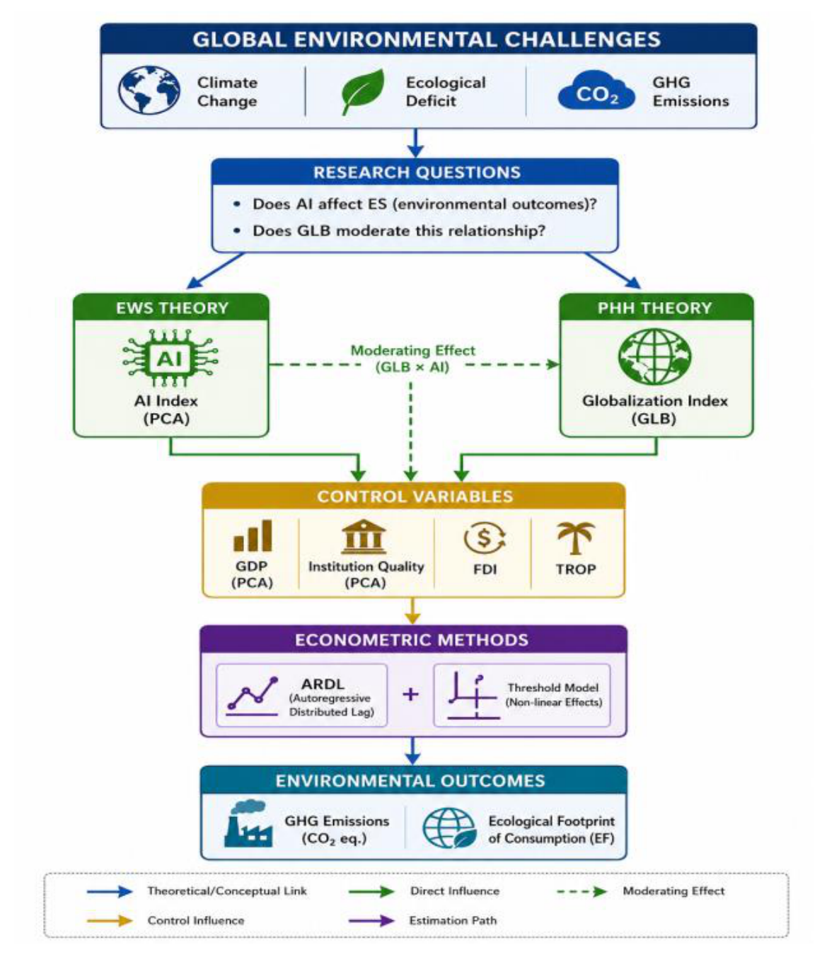
Figure 2.
Pollution haven or halo theory. Source: Abbasi et al [41].
Figure 2.
Pollution haven or halo theory. Source: Abbasi et al [41].
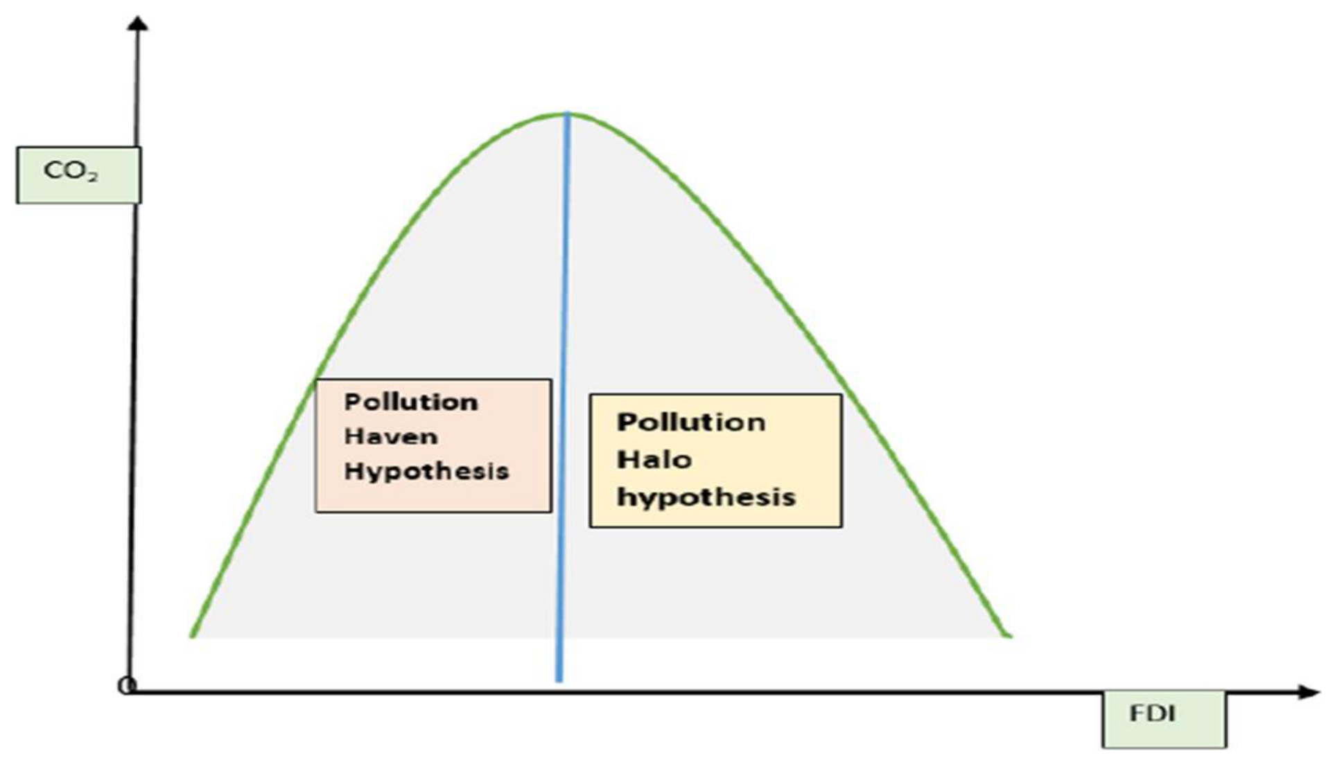
Figure 3.
Illustration of direct and indirect demand for domestic and global biocapacity. Source: Borucke et al. [53].
Figure 3.
Illustration of direct and indirect demand for domestic and global biocapacity. Source: Borucke et al. [53].
Figure 4.
Relationship between ecological footprint of consumption and greenhouse gas emissions. Source: Authors.
Figure 4.
Relationship between ecological footprint of consumption and greenhouse gas emissions. Source: Authors.
Figure 5.
LR diagram of first and second TV test for models 1 and 2. Source: Authors
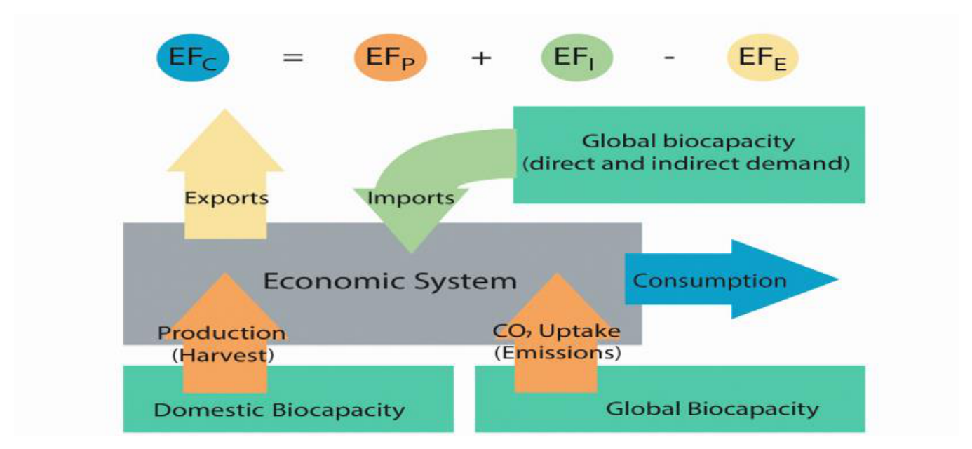
Figure 6.
The role of globalization in the relationship between artificial intelligence index and ecological footprint of consumption. Note: Optimal threshold at globalization= 08172. Source: Authors.
Figure 6.
The role of globalization in the relationship between artificial intelligence index and ecological footprint of consumption. Note: Optimal threshold at globalization= 08172. Source: Authors.
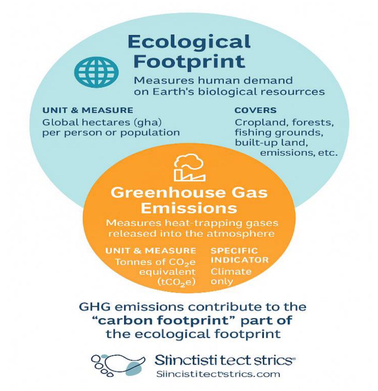
Figure 7.
The role of globalization in the relationship between artificial intelligence index and greenhouse gas emissions. Note: Optimal threshold at globalization= 08052. Source: Authors.
Figure 7.
The role of globalization in the relationship between artificial intelligence index and greenhouse gas emissions. Note: Optimal threshold at globalization= 08052. Source: Authors.
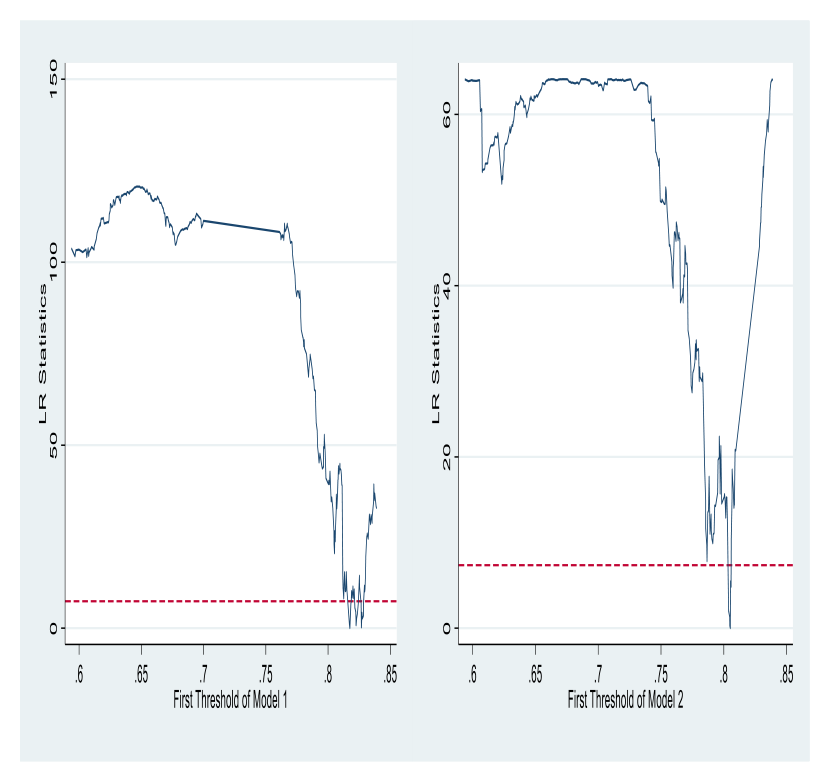
Table 1.
Variables descriptions and sources.
| Variables | Descriptions | Source |
|---|---|---|
| Dependent variables | ||
| Ecological Footprint of Consumption (EFC) | EFC measures the environmental impact of human activities by assessing the demand placed on natural resources relative to the Earth's capacity to regenerate those resources. It serves as a useful indicator for comparing human resource consumption with the planet’s renewable supply. | Global Footprint Network (GFN) |
| Greenhouse Gas emissions Per Capita (GHGPC) | Human-caused greenhouse gas (GHG) emissions drive climate change. GHG emissions are gases in Earth’s atmosphere that trap heat, contributing to the greenhouse effect, which leads to global warming and climate change. | WDI |
| Explanatory variables | ||
| Artificial Intelligence (AIx) | A comprehensive AI evaluation index, constructed using the PCA method, based on four dimensions: AI-related technology, network infrastructure, international competitiveness of digital products, and government institutional support. | Authors’ calculations |
| Economic Development (ED) | GDP per capita (in constant 2015 U.S. dollars), representing the inflation-adjusted value of goods and services produced per person. | WDI |
| Control Variables | ||
| Foreign Direct Investment (FDI) | Foreign direct investment, net inflows (% of GDP) measures the value of inward direct investment made by non-resident investors, expressed as a percentage of a country’s GDP. It reflects the acquisitions of at least a 10% ownership stake in enterprises operating within an economy other than that of the investor, indicating long-term management interest and control. | |
| Trade Openness (TROP) | Trade is the sum of exports and imports of goods and services measured as a share of gross domestic product. | |
| Institutional Quality (IQx) | A comprehensive Governance index, constructed using the PCA method, based on: Control of Corruption, Government Effectiveness, Political Stability and Absence of Violence/Terrorism, Regulatory Quality captures perceptions, Rule of Law captures and Claims on central government. | WGI, Authors’ calculations |
| Moderating variable | ||
| Globalization (GLB) | KOF GLB Index encompasses three key dimensions- economic globalization, social globalization, and political globalization- offering a comprehensive assessment of a country's global integration over time. | KOF |
Source: Authors.
Table 2.
The different components of ecological footprint of consumption.
| EF of Consumption () | EF of Production () | Net EF of Trade ( |
|---|---|---|
| The EF of consumption indicates the consumption of biocapacity by a country’s inhabitants. In order to assess the total domestic demand for resources and ecological services of a population, the EF of consumption () is used. accounts for both the export of national resources and ecological services for use in other countries, and the import of resources and ecological services for domestic consumption. is most amenable to change by individuals through changes in their consumption behavior. |
The EF of production indicates the consumption of biocapacity resulting from production processes within a given geographic area, such as a country or region. It is the sum of all the bio productive areas within a country necessary for supporting the actual harvest of primary products (cropland, grazing land, forestland, and fishing grounds), the country’s built-up area (roads, factories, cities), and the area needed to absorb all fossil fuel carbon emissions generated within the country. This measure mirrors the gross domestic product (GDP), which represents the sum of the values of all goods and services produced within a country’s borders. |
The EF of imports and exports indicates the use of biocapacity within international trade. Embedded in trade between countries is a use of biocapacity, the net EF of trade (the EF of imports minus the EF of exports). If the EF embodied in exports is higher than that of imports, then a country is a net exporter of renewable resources and ecological services. Conversely, a country whose Footprint of imports is higher than that embodied in exports depends on the renewable resources and ecological services generated by ecological assets from outside its geographical boundaries. |
Note: Data and Methodology - Global Footprint Network. Source: Authors.
Table 3.
The different components of greenhouse gas emissions.
| Components | Main sources of emissions | Characteristics |
|---|---|---|
| Carbon Dioxide (CO2) | Burning fossil fuels (coal, natural gas, oil), solid waste and biomass reactions (cement production). | Removed from the atmosphere by plant absorption as part of the biological carbon cycle. |
|
Methane (CH4) |
Production and transport of coal, natural gas and oil, livestock, agriculture, land use and decay of organic waste in landfills. | More potent than CO₂ in terms of warming potential; significant agricultural emissions. |
| Nitrous Oxide (N2O) | Agricultural activities, land use, industry, combustion of fossil fuels and solid waste, wastewater. | Powerful greenhouse gas; emissions mainly from agriculture and waste treatment. |
| Other components | Fluorinated gases, solid and liquid aerosols, and certain additional greenhouse gases such as water vapor and tropospheric ozone. | |
Source: Authors.
Table 4.
Artificial intelligence index selection.
| Core Indicators | Basic indicators | Sources |
|---|---|---|
| AI-related technology | Number of industrial robots deployed | IFR |
| Network infrastructure (ICT) | Fixed Broadband Access per 100 Individuals | WDI |
| Fixed-Line Telephone Subscriptions per 100 Inhabitants | WDI | |
| Percentage of individuals using the Internet | WDI | |
| Government institutional support | E-participation | United Nations e-government survey |
| Online service | United Nations e-government survey | |
| E-governance | United Nations e-government survey |
Source: Authors.
Table 6.
Descriptive statistics.
| Variable | Mean | Median | Min | Max | SD | CV | Skewness | Kurtosis |
|---|---|---|---|---|---|---|---|---|
| LEFC | 0.6273 | 0.6599 | -0.1249 | 1.6401 | 0.2561 | 0.4083 | -0.1398 | 4.4608 |
| LGHGPC | 0.8630 | 0.8859 | -1.0457 | 1.5697 | 0.3048 | 0.3531 | -0.9282 | 6.1917 |
| LAIx | 1.8146 | 1.8964 | 0.2794 | 2.7931 | 0.3340 | 0.1841 | -1.7965 | 7.8533 |
| LED | 4.1559 | 4.2083 | 2.8789 | 4.9881 | 0.4718 | 0.1135 | -0.3423 | 2.0556 |
| LFDI | 1.6507 | 1.6395 | -0.0392 | 2.1690 | 0.0860 | 0.0521 | -5.7325 | 126.728 |
| LTROP | 1.9006 | 1.8957 | 1.29136 | 2.6408 | 0.2414 | 0.1270 | 0.2005 | 3.0317 |
| IQx | 1.0425 | 1.0269 | -5.4462 | 4.9991 | 1.7132 | 1.6433 | -0.0433 | 2.3232 |
| GLB | 0.7358 | 0.7562 | 0.3776 | 0.91 | 0.1108 | 0.1506 | -0.5940 | 2.8466 |
Source: Authors.
Table 7.
Correlation matrix and VIF.
| Variable | LEF | LGHGPC | LAIx | LED | LFDI | LTROP | IQx | GLB | Mean VIF |
|---|---|---|---|---|---|---|---|---|---|
| LEFC | 1.0000 | ||||||||
| LGHGPC | 0.6512 | 1.0000 | |||||||
| LAIx | 0.3866 | 0.2926 | 1.0000 | ||||||
| LED | 0.8094 | 0.5931 | 0.5157 | 1.0000 | |||||
| LFDI | 0.0858 | 0.0508 | -0.0010 | 0.0727 | 1.0000 | ||||
| LTROP | 0.2381 | 0.0210 | 0.0758 | 0.1512 | 0.2593 | 1.0000 | |||
| IQx | 0.6968 | 0.3772 | 0.3454 | 0.7763 | 0.1344 | 0.2289 | 1.0000 | ||
| GLB | 0.5696 | 0.3825 | 0.5417 | 0.7954 | 0.0920 | 0.2920 | 0.7200 | 1.0000 | |
| VIF Test | 1.51 | 3.85 | 1.08 | 1.20 | 2.85 | 3.44 | 2.32 |
Source: Authors.
Table 8.
Cross-section dependence tests.
| Method 1: CD-Test of All Variables | Crit-Val |
|---|---|
| LEFC | 22.624*** |
| LGHGPC | 10.105*** |
| LAIx | 199.894*** |
| LED | 154.572*** |
| LFDI | 22.7*** |
| LTROP | 46.573*** |
| IQx | -0.607 |
| GLB | 176.516*** |
| Method 2: CD-Tests by model | |
| Model 1: EFC | |
| Pesaran | 42.604*** |
| Friedman | 307.749*** |
| Frees | 14.731*** |
| Model 2: GHGPC | |
| Pesaran | 29.277*** |
| Friedman | 208.712*** |
| Frees | 19.046*** |
Note: ***, ** and * indicate statistical significance at 1%, 5% and 10%. Source: Authors.
Table 9.
Panel unit root tests result.
| IPS of first generation | CIPS of second generation | |||
|---|---|---|---|---|
| Variables | At level | At first difference | At level | At first difference |
| LEFC | -3.079*** | -22.716*** | -2.247*** | -5.161*** |
| LGHGPC | 2.383 | -18.190*** | -1.119 | -4.448*** |
| LAIx | -13.403*** | -8.809*** | -3.163*** | -4.167*** |
| LED | 0.690 | -13.887*** | -1.638 | -2.976*** |
| IQx | 0.685 | -16.359*** | -1.495 | -4.466*** |
| LFDI | -9.242*** | -25.889*** | -3.616*** | -5.501*** |
| LTROP | -0.298 | -18.858*** | -1.828 | -3.902*** |
Note: ***, ** and * indicate statistical significance at 1%, 5% and 10%. Source: Authors
Table 10.
Cointegration tests results.
| Tests | Model 1: EFC | MODEL 2: GHGPC |
|---|---|---|
| Seven tests of Peter Pedroni | Statistic | Statistic |
| Between-dimension | ||
| Rho | 5.6184*** | 7.7244*** |
| PP | -10.2181*** | -2.3530*** |
| ADF | -10.7494*** | -2.5008*** |
| Within-dimension | ||
| V | -4.4797*** | -5.1844*** |
| Rho | 4.2498*** | 5.7225*** |
| PP | -5.7312*** | -0.4679 |
| ADF | -4.8645*** | -0.5395 |
| Five tests of Kao | ||
| MDF | 6.007*** | 4.331*** |
| DF | 4.794*** | 4.201*** |
| ADF | 9.397*** | 15.031*** |
| UMDF | -24.215*** | -1.445 |
| UDF | -17.985*** | -1.498 |
| Westerlund test | ||
| Gt | -2.625*** | -1.953*** |
| Ga | -6.209 | -4.674 |
| Pt | -22.915*** | -14.674 *** |
| Pa | -6.432*** | -4.496 |
Note: ***, ** and * indicate statistical significance at 1%, 5% and 10%. Source: Authors.
Table 12.
Analysis of the ecological world-systems theory by PMG-method.
| Variables | Model 1: EFC | Model 2: GHGPC | |
|---|---|---|---|
| Coefficients | Coefficients | ||
| Long-run equation (ec) | |||
| LAIx | -0.055*** | -0.028*** | |
| LED | 0.553*** | 0.441*** | |
| LTROP | -0.130*** | 0.193*** | |
| IQx | 0.048*** | 0.001 | |
| Short-run equation (SR) | |||
| ec | -0.383*** | -0.484*** | |
| D1.LAIx | 0.243*** | 0.382** | |
| D1.LED | 0.741*** | -0.389*** | |
| LTROP | 0.118*** | 0.185*** | |
| D1. IQx | -0.007 | 0.028 | |
| Hausman MG -PMG | |||
| Prob > chi2 | 9.65** | 10.30*** | |
| Hausman DFE -PMG | |||
| Prob > chi2 | 50.92*** | 7.55 | |
Note: ***, ** and * indicate statistical significance at 1%, 5% and 10%. Source: Authors.
Table 14.
Results of threshold value.
| Model | Threshold estimator (level = 95) | |||||
| Model 1: EFC | Model 2: GHGPC | |||||
| Threshold | Lower | Upper | Threshold | Lower | Upper | |
| Th-1 | 0.8175 | 0.8157 | 0.8183 | 0.8052 | 0.8039 | 0.8054 |
Source: Authors.
Table 15.
Results of thresholds effect.
| Threshold | Model 1: EFC | Model 2: GHGPC | ||||||||
| F-stat | Prob | Crit 10% | Crit 5% | Crit 1% | F-stat | Prob | Crit 10% | Crit 5% | Crit 1% | |
| Single | 109.37 | 0.000*** | 51.892 | 62.540 | 86.866 | 17.973 | 0.012*** | 54.782 | 66.839 | 90.053 |
Note: ***, ** and * indicate statistical significance at 1%, 5% and 10%. Source: Authors.
Table 16.
Threshold regression results.
| Variables | Model 1: EFC | Model 2: GHGPC |
|---|---|---|
| LED | 0.304*** | 0.405*** |
| LTROP | -0.038 | -0.001 |
| LFDI | 0.052*** | 0.078** |
| GLB | -0.275*** | 0.676** |
| LAIx (GLB≤= 0.8175) | 0.017* | |
| LAIx (GLB>=0.8175) | -0.019* | |
| LAIx (GLB≤=0.8052) | -0.070*** | |
| LAIx (GLB>=0.8052) | -0.132*** | |
| Constant | -0.457*** | -1.281*** |
Note: ***, ** and * indicate statistical significance at 1%, 5% and 10%. Source: Authors.
Disclaimer/Publisher’s Note: The statements, opinions and data contained in all publications are solely those of the individual author(s) and contributor(s) and not of MDPI and/or the editor(s). MDPI and/or the editor(s) disclaim responsibility for any injury to people or property resulting from any ideas, methods, instructions or products referred to in the content. |
© 2026 by the authors. Licensee MDPI, Basel, Switzerland. This article is an open access article distributed under the terms and conditions of the Creative Commons Attribution (CC BY) license (http://creativecommons.org/licenses/by/4.0/).
Copyright: This open access article is published under a Creative Commons CC BY 4.0 license, which permit the free download, distribution, and reuse, provided that the author and preprint are cited in any reuse.