Submitted:
13 June 2026
Posted:
15 June 2026
You are already at the latest version
Abstract
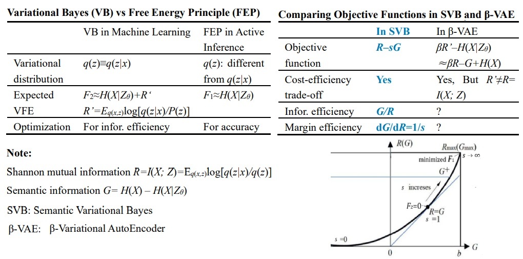
Friston et al.’s minimum Free Energy Principle (FEP) concludes that the Expected Variational Free Energy (EVFE) indicates both predictive inaccuracy and average surprise. It is incorrect to say that EVFE implies inaccuracy, as it stems from differences between the variational distributions used by FEP and Variational Bayes (VB). VB treats the variational distribution q(z) as a shorthand for the posterior distribution q(z|x), and the EVFE F2 approximates the cross-entropy and implies average surprise. However, in FEP, q(z) and q(z|x) differ; the EVFE F1 approximates the conditional cross-entropy and reflects predictive inaccuracy. Because of F2 = F1 + R (R is Shannon mutual information), using F2 minimizes both error and information cost R, while using F1 ignores information efficiency, so that Active Inference based on FEP is equivalent to Error Control. The author has previously proposed Semantic Variational Bayes (SVB) based on the study of semantic information theory (including the R(G) function) (R(G) is the minimum R for given semantic information G). SVB uses the information difference IND = R – sG as the objective function, where G = H(x) – F2. When s=1, minimizing IND is equivalent to minimizing F2. Using s allows us to balance between maximum semantic information (G) and maximum information efficiency (G/R). Two computational examples illustrate that minimizing F1 and minimizing F2 yield different optimized q(z|x); that F1 can increase as F2 decreases; and that using F1 only focuses on prediction accuracy. Clarifying these problems with FEP and VB should help understand and improve them.
Keywords:
variational bayes
; minimum free energy principle
; mutual information
; semantic information
; maximum information efficiency
; active inference
1. Introduction
The Variational Bayesian method (VB) developed by Hinton et al. [1,2,3] has greatly promoted unsupervised learning and deep learning. Hinton’s Nobel Prize in Physics was related to his proposal of Variational Free Energy (VFE) as the optimization criterion of VB. Friston et al. applied VB to research in fields such as neuroscience and further developed the minimum Free Energy Principle (FEP) [4]. To clarify the task, Friston et al. developed Active Inference based on FEP and published many articles [5,6] introducing its applications in fields such as neuroscience and biological self-organization. FEP has had a great impact, to the point that we often see FEP workshops or learning organizations.
The author has pointed out the shortcomings of FEP (such as the contradiction between the concept of Variational Free Energy (VFE) and the concept of physical free energy) and has improved FEP to the Maximum Information Efficiency Principle [7]. At that time, the author thought that VB made the mixture model converge because it used the mean-field approximation, making the actual variation become a posterior distribution q(z|x) instead of a prior distribution q(z) (x is the observed datum, z is the latent variable). The author didn’t realize that the VFE used by Friston et al. was different from the VFE in VB. Recently, I discovered that because Friston et al. used a different VFE, they concluded that the expected VFE reflects both the average surprise of x (approximating the cross-entropy Hθ(x)) and the predictive inaccuracy (approximating the conditional cross-entropy Hθ(x|z), where z is the latent variable). However, this conclusion is wrong because Hθ(x) and Hθ(x|z) usually differ obviously.
In VB, q(z) is a shorthand for q(z|x) [2,3,8]. Whether or not q(z) is considered a shorthand for q(z|x) leads to two different variational free energies. In most of Friston et al.’s papers, the variational distribution used is q(z), different from q(z|x), so their VFE reflects predictive inaccuracy. They also accepted the VB’s conclusion: the expected VFE approximates the cross-entropy Hθ(x), thus leading to the aforementioned erroneous conclusion.
On the other hand, in VB, q(z) and q(z|x) are not distinguished, making it impossible to express Shannon mutual information as an information cost, thereby obscuring the idea of maximum information efficiency contained in the minimum VFE criterion.
Based on the semantic information G theory [9], the author proposed Semantic Variational Bayes (SVB) [10], in which the objective function is essentially the same as that in VB. This paper discusses FEP, VB, and SVB together, thereby deepening our understanding of them.
This paper aims to:
- 1) Analyze the error in FEP and its mathematical cause.
- 2) Clarify the equivalence relationship between the minimum free energy criterion and the maximum information efficiency criterion to promote the application of the maximum information efficiency criterion.
VB has a significant impact on machine learning, and the FEP also has a wide influence on research on brain neurons and biological self-organization. It is of great importance to clarify and improve them.
2. Two Expected VFEs and the Mathematical Cause of the above Error
In VB, the common formula for VFE is:
where P(x, z)=Pθ(x, z)= P(x, z|θ) (i.e, P(y, x|C) or P(o, s|C) in Friston et al.’s book [6]), q(z) is constructed using the parameter π,i.e., q(z) = q(x|π) = qπ(z). Whether or not q(z) is considered as a shorthand for the posterior distribution q(z|x) will result in two different expected VFEs: F1 and F2.
In VB, q(z) is a shorthand for q(z|x), i.e, q(z)=q(z|x),and hence, the expected VFE is actually:
where ΔR approaches 0 after optimization, so F2 is close to the cross-entropy Hθ(x).
However, in FEP, q(z) is usually not a shorthand for q(z|x), i.e., q(z) ≠ q(z|x) (evidence will be provided later). If q(z) ≠ q(z|x), then the expected VFE is...
Obviously, R’ is close to the Shannon mutual information and will not be equal to 0. Therefore, F1 will not be close to the cross-entropy Hθ(x). The above formula can also be written as:
where P(x|z) is the likelihood function, i.e., P(x|z)=P(x|z, θ)=P(x|zθ). Because DKL(.) in the above formula is close to 0 after optimization, F1 is close to the conditional cross-entropy Hθ(x|z), implying predictive inaccuracy. The relationship between F1 and F2 is:
where R is the Shannon mutual information.
F2 = R + F1,
Why did Friston et al. conclude that F1 implies both the inaccuracy Hθ(x|z) and the average surprise Hθ(x)? This is because, in interpreting R’, they also treated q(z) as the conditional posterior distribution q(z|x) (see [6], p. 51). The problem is: if q(z) = q(z|x), DKL(q(z)||P(z)) in Eq. (4) will not be close to 0, meaning F1 ≠ Hθ(x|z). Therefore, saying F1 ≈ Hθ(x|z) ≈ Hθ(z) ≈ F2 is because of the inconsistent interpretation of q(z). Because the information term ΔR in F2 is close to 0, whereas the information term –R1 in F1 is negative and not close to 0, it is incorrect to say that F1 is simultaneously close to both Hθ(x|z) and Hθ(x). According to many formulas derived by Friston et al., they did not treat q(z) as a shorthand for q(z|x) in most cases; q(z) represents the prior distribution, not the posterior distribution. The reasons are
- Friston also confirmed in his correspondence with the author that the expected VFE is F1.
- Friston agreed in his reply that the author interpreted H(x) – F1 as semantic mutual information, which implies that the expected VFE he uses is close to Hθ(x|z).
Why is FEP effective in many applications? The reasons are:
- In machine learning, it uses the maximum likelihood criterion for the optimization of the model parameter θ;
- In Active Inference, minimizing F1 is equivalent to minimizing average error.
For example, if P(x|zθj) is a normal distribution exp[–(x-xj)2], then Hθ(x|z) is the average squared error. Thus, minimizing F1 or Hθ(x|z) is equivalent to minimizing the average squared error, and hence, Active Inference becomes Error Control. However, in this way, the pursuit of maximum information efficiency contained in VB does not exist. Although Friston et al. sometimes say that FEP considers information efficiency [14], the formula they use to explain information efficiency is Eq. (4), in which DKL(q(z)||P(z)) may be close to 0 after optimization, so it is not Shannon mutual information as a cost.
3. Equivalence Relation and Differences Between VB and SVB
Based on the semantic information G theory, the author proposed SVB, where semantic or predictive information is
G = I(x;zθ) = H(x) – Hθ(x|z) ≈ H(x) – F1.
Extending the information rate distortion function R(D) [13], given the semantic mutual information G, we find the minimum Shannon mutual information to obtain the R(G) function. The objective function used is the information difference:
IND = R – s G.
Finding the minimum R is equivalent to finding the maximum information efficiency, f = G/R. When s = 1, the maximum information efficiency can reach 1. At this time, the relationship between IND and F2 can be found from the following formula:
Because DKL(.) above is close to 0, and H(x) is a constant, minimizing F2 is equivalent to minimizing the information difference R – G or maximizing the information efficiency G/R.
The difference is that in SVB, the use of s allows us to make a trade-off between maximum semantic information and maximum information efficiency. Furthermore, SVB allows us to use not only the likelihood function P(x|zθ) as a constraint, but also truth, membership, similarity, and distortion functions as constraints [10]. Solving for q(z|x) and q(z) in SVB is also very simple; we can obtain the optimized q(z|x) and q(z) by alternating between q(z|x) and q(z) as variations. The iterative formulas are:
where mij=P(xi|zθj)/P(xi)=T(zθj|x)/T(zθj), T(zθj|x) is the truth, membership, similarity, or distortion function, and T(zθj) is the mean or the logical probability.
Higgins et al. [14] also found the relationship between VFE and information efficiency. They proposed β-VAE [14] for deep learning, which has yielded significant progress. The β-VAE combines the advantages of maximum entropy theory and VB, and its objective function to be maximized is:
where the DKL(.) term can be viewed as information cost, but its average is not Shannon mutual information. This is because Shannon’s mutual information is:
L = Eq π(z|x) [log P(x|z)] − β DKL(qπ(z|x)||p(z)) ,
R = I(x;z) = Eq(x,z)log[q(z|x)/q(z)].
Comparing the objective functions in Eqs. (6) and (7), we can see that in SVB, Shannon mutual information (as the cost), semantic mutual information (as the utility), and information efficiency (G/R) can all be easily calculated. However, in VB and β-VAE, these cannot be calculated.
4. Experimental Results
4.1. Performances of q(z|x) and F1 Under Different Tasks
Regardless of the task, minimizing F2 requires q(x|zj)=P(x|zθj) or q(zj|x)=Pθ(x,zj)/ Pθ(x)(j=1,2,…), making F2 close to H(x). However, q(z|x) behaves differently when minimizing F1 across various tasks.
Let Pθ(x) be a mixture of two Gaussian distributions (see Figure 1) to approximate a sampling distribution P(x) produced by a true mixture model. In the true model, the two means are c1=40, c2=75,two standard deviations are σ1=15, σ2=10, mixture ratios are P(z1)=0.7, P(z2)=0.3, x=1,2,…,100.
The required q*(z|x) for the mixture model is shown in Figure 1. Currently, R(s=1) = G(s=1) = 0.621 bits (see Table 1 for details).
For the mixture model, minimizing F1 requires P(x|zθj) = q(x|zj) (j=1,2…). At this point, F1 approaches the Shannon conditional entropy, i.e., F1=H(x|zθ) ≈ H(x|z).
Figure 3 shows the required q*(z|x), which minimizes F1, without requiring Pπ(x)≈P(x). This indicates that Active Inference becomes Error Control.
Table 1 shows that, across the three tasks, the optimized increases successively, while and G/R
decrease successively.
4.2. F2 Decreases While F1 Increases During a Mixture Model’s Convergence
When solving the mixed model, we need to minimize F2. Usually, people assume that F1 and F2 decrease at the same time, so they do not distinguish between the two. However, there is a typical counterexample (see Table 2 and Figure 4), in which F1 increases when F2 decreases.
In this example, during the convergence, F2 decreases while F1 increases.
5. Discussion
Friston et al. wrongly concluded that the expected VFE, in addition to representing average surprise, also indicates predictive inaccuracy. The root of the error lies in the fact that, unlike VB, FEP does not use q(z) as the posterior distribution q(z|x). The example in Section 4.1 shows that different tasks may require different variational distributions and that the optimized q(z|x) may differ. Using F1 as the expected VFE, Active Inference becomes Error Control, and the pursuit of information efficiency in VB no longer exists.
The example in Section 4.2 shows that minimizing F2 may increase F1, and the two expected VFEs are not always positively correlated. This fact reminds us that we must distinguish between the two.
The mathematical analysis in Section 3 shows that, to combine the advantages of the maximum entropy method, the maximum information efficiency criterion does not simply maximize information efficiency. For some tasks (such as data compression and constraint control), we need a trade-off between the maximum semantic information and the maximum information efficiency. Compared with VB and β-VAE, SVB can calculate information efficiency and provides a more intuitive method for the trade-off (using the function R(G(s)) [7]).
Following Friston et al., who use FEP to explain mutual adaptation between organisms and environments and biological self-organization, we can also use the maximum information efficiency principle [7] to explain them. The different conclusion is that, in the process of adapting to their environment, bio-organisms do not pursue minimum error or maximum semantic information (utility), but rather weigh semantic information against Shannon’s information (cost), or against information efficiency.
6. Conclusions
Using different variational distributions yields different expected VFEs: F1 (close to the conditional cross-entropy) and F2 (close to the cross-entropy). In deep learning, Hinton et al. minimized F2, which is equivalent to minimizing the information difference R–G or maximizing the information efficiency G/R. However, in Friston et al.’s FEP and Active Inference, F1 is usually minimized, which is equivalent to minimizing prediction error or maximizing semantic or predictive information. Because F1 loses the information term from F2, it no longer reflects VB’s focus on information cost and information efficiency. Friston et al.’s distinction between the two variational distributions helps express Shannon’s mutual information and semantic mutual information, but the assertion that VFE implies both predictive inaccuracy and surprise is incorrect because they interpret the variational distributions inconsistently.
The objective function used by Higgins et al. in β-VAE combines the advantages of VB and the Maximum Entropy method; the objective function used in the SVB proposed by the author of this paper is R–sG. The two objective functions are similar, but in SVB, we can calculate cost information R, semantic information G, and information efficiency G/R, which makes it easier to balance between minimum cost information R and maximum utility information G, or between maximum utility information G and maximum information efficiency G/R.
References
- Hinton, G.E.; van Camp, D. Keeping the neural networks simple by minimizing the description length of the weights. In Proceedings of the 6th Annual Conference on Computational Learning Theory, 1993; pp. 5–13. [Google Scholar]
- Hinton, G.E.; Zemel, R.S. Autoencoders, minimum description length and Helmholtz free energy. In Proceedings of the 6th International Conference on Neural Information Processing Systems, 1993; pp. 3–10. [Google Scholar]
- Neal, R.M.; Hinton, G.E. A view of the EM algorithm that justifies incremental, sparse, and other variants. In Learning in Graphical Models; Jordan, M.I., Ed.; MIT Press: Cambridge, MA, 1999; pp. 355–368. [Google Scholar]
- Friston, K. The free-energy principle: A unified brain theory? Nat. Rev. Neurosci. 2010, 11, 127–138. [Google Scholar] [CrossRef] [PubMed]
- Friston, K.J.; Parr, T.; de Vries, B. The graphical brain: Belief propagation and active inference. Netw. Neurosci. 2017, 1, 381–414. [Google Scholar] [CrossRef] [PubMed]
- Parr, T.; Pezzulo, G.; Friston, K.J. Active Inference: The Free Energy Principle in Mind, Brain, and Behavior; MIT Press: Cambridge, MA, 2022. [Google Scholar]
- Lu, C. Improving the minimum free energy principle to the maximum information efficiency principle. Entropy 2025, 27, 684. [Google Scholar] [CrossRef] [PubMed]
- Nguyen, D. An in Depth Introduction to Variational Bayes Note. Available at. 2023. [Google Scholar] [CrossRef]
- Lu, C. A semantic generalization of Shannon’s information theory and applications. Entropy 2025, 27, 461. [Google Scholar] [CrossRef] [PubMed]
- Lu, C. Semantic Variational Bayes Based on Semantic Information G Theory for Solving Latent Variables. J. Electron. Inf. Syst. 2026, 8(1), 30–46. [Google Scholar] [CrossRef]
- Sengupta, B.; Stemmler, M.B.; Friston, K.J. Information and efficiency in the nervous system—A synthesis. PLoS Comput. Biol. 2013, 9, e1003157. [Google Scholar] [CrossRef] [PubMed]
- Da Costa, L.; Parr, T.; Sajid, N.; Veselic, S.; Neacsu, V.; Friston, K. Active inference on discrete state-spaces: A synthesis. J. Math. Psychol. 2020, 99, 102447. [Google Scholar] [CrossRef] [PubMed]
- Shannon, C.E. Coding theorems for a discrete source with a fidelity criterion. In IRE National Convention Record; 1959; pp. 142–163. [Google Scholar]
- Higgins, I.; Matthey, L.; Pal, A.; Burgess, C.; Glorot, X.; Botvinick, M.; Mohamed, S.; Lerchner, A. Beta-VAE: Learning basic visual concepts with a constrained variational framework. In Proceedings of the International Conference on Learning Representations (ICLR), 2017. [Google Scholar]
Figure 1.
The variational distribution q(z|x) was optimized for the mixture model with F2=0 and G/R=1, where s=1 and Pπ(x) ≈ Pθ(x) ≈ P(x).
Figure 1.
The variational distribution q(z|x) was optimized for the mixture model with F2=0 and G/R=1, where s=1 and Pπ(x) ≈ Pθ(x) ≈ P(x).

Figure 2.
The variational distribution q(x|z) was optimized for the classification with a minimum and maximum , where s→∞ and Pπ(x) ≈ Pθ(x) ≈ P(x).
Figure 2.
The variational distribution q(x|z) was optimized for the classification with a minimum and maximum , where s→∞ and Pπ(x) ≈ Pθ(x) ≈ P(x).

Figure 3.
The q(z|x) was optimized for minimum F1 and maximum G, where Pπ(x)= q(z1|x) = δ(75), without requiring Pπ(x) ≈ Pθ(x).
Figure 3.
The q(z|x) was optimized for minimum F1 and maximum G, where Pπ(x)= q(z1|x) = δ(75), without requiring Pπ(x) ≈ Pθ(x).

Figure 4.
The convergence process of the mixture model. Q is the complete data log likelihood.


Table 1.
Changes of optimized , , , and across the three tasks.
| Task | Requirements | R(bits) | G(bits) | F1(bits) | G/R |
| Mixture model, minimizing F2 |
s=1, R=G, Hθ(x)≈H(x)=6.38 |
0.621=G | 0.621 | 5.76 | 1.0 |
| Classification, minimizing F1 |
s→∞, Hθ(x)≈H(x) | 0.954=H(z) | 0.80 | 5.58 | 0.84 |
| Active Inference, minimizing F1 |
Ha(x)≠H(x), H(X|Z)=0 |
6.38=H(x) | 1.62 | 4.76 | 0.25 |
Table 2.
True parameters and Initial parameters of the Mixture Model.
| True model’s Parameters | Initial parameters | ||||||
| c* | σ* | P*(Y) | c | σ | P(Y) | ||
| y1 | 40 | 15 | 0.5 | 40 | 5 | 0.5 | |
| y2 | 75 | 15 | 0.5 | 40 | 5 | 0.5 | |
Note that the initial σj is much smaller than the convergent σj (j=1,2), which is the reason that F1 increases and Q decreases (Q is the complete data log-likelihood).
Disclaimer/Publisher’s Note: The statements, opinions and data contained in all publications are solely those of the individual author(s) and contributor(s) and not of MDPI and/or the editor(s). MDPI and/or the editor(s) disclaim responsibility for any injury to people or property resulting from any ideas, methods, instructions or products referred to in the content. |
© 2026 by the authors. Licensee MDPI, Basel, Switzerland. This article is an open access article distributed under the terms and conditions of the Creative Commons Attribution (CC BY) license (http://creativecommons.org/licenses/by/4.0/).
Copyright: This open access article is published under a Creative Commons CC BY 4.0 license, which permit the free download, distribution, and reuse, provided that the author and preprint are cited in any reuse.


