

Submitted:
12 June 2026
Posted:
12 June 2026
You are already at the latest version
Abstract
Learning from High-Dimensional Low-Sample Size data has long been a persistent challenge in machine learning, because models must infer reliable patterns from limited observations while handling a large number of variables,this challenge is especially common in biomedical applications. High-dimensional small-sample data make predictive modeling vulnerable to unstable training and overfitting. To address this issue, we propose GINet-DGC, an AI framework that integrates feature-wise structural priors with dynamic generalization monitoring. Instead of directly learning an unconstrained first-layer weight matrix, GINet-DGC generates task-specific weights from multi-view feature descriptors, including latent semantic, global distributional, local topological, and hierarchical representations. This structure-constrained weight generation design narrows the feature-interaction search space and acts as an inductive regularizer against noise and redundant molecular features. Furthermore, we introduce an Overfitting-aware Index to monitor the training trajectory and detect the generalization saturation point for adaptive termination. Experiments on eight publicly accessible real-world biomedical HDLSS gene-expression datasets, evaluated under repeated stratified 5×5 cross-validation, show that GINet-DGC achieves competitive and stable performance against 17 baselines. These results suggest that explicitly encoding structural priors can improve robust AI modeling for data-scarce benchmarks.
Keywords:
high-dimensional low-sample size
; tabular representation learning
; structure-constrained weight generation
; dynamic generalization control
1. Introduction
This section presents a general overview of the study by outlining the background, reviewing related works, identifying the research gaps, and summarizing the main contributions of this research.
1.1. Background and Motivation
Tabular data are among the most widely used data forms in scientific computation and industrial analysis because they naturally represent heterogeneous observations through structured variables. These data routinely play an important role in supporting advanced research in high-energy physics [1], computational chemistry [2], and financial forecasting [3]. Beyond these fields, structured variables are particularly crucial for predictive modeling and knowledge discovery in biomedicine and health-oriented artificial intelligence [4,5]. However, across many of these scientific disciplines, informative datasets are difficult to collect because experiments can be costly, time-consuming, or ethically constrained. For example, in experimental particle physics, high-dimensional detector measurements are produced under highly costly acquisition conditions [6].This data scarcity becomes even more severe in biomedical gene-expression analysis. Within typical transcriptomic arrays, a single spreadsheet routinely contains tens of thousands of molecular features against merely dozens or hundreds of clinical patient samples [7]. This severe mathematical discrepancy in scale precisely defines the High-Dimensional Low-Sample Size (HDLSS) nature of the data, creating a heavily asymmetrical dataset. Consequently, researchers must infer reliable patterns under an extreme regime where the feature dimension greatly exceeds the number of available observations [8,9]. In this scenario, limited samples provide insufficient supervision for the massive parameter space of deep learning models. This optimization constraint frequently makes traditional networks vulnerable to stochastic noise, feature redundancy, and unstable gradients, potentially leading to severe overfitting.
Achieving effective inference from such data is thus a pressing challenge in modern machine learning and a key step toward empirical scientific discovery. In this study, we focus on biomedical gene-expression classification, which is widely recognized as a highly typical problem within the HDLSS learning scenario.
1.2. Related Works
This section reviews existing literature to clarify the scope of current paradigms and highlight the open challenges that motivate this study.
In the context of small-sample tabular learning, traditional tree-based ensemble methods and shallow models with regularization remain the most competitive and stable baselines [9].Representative models such as XGBoost [10] and LightGBM [11] achieve good generalization through efficient feature splitting and regularized ensemble learning. However, tree-based models cannot perform end-to-end representation learning, which restricts their ability to capture complex, high-order dependencies among molecular features. To address these limitations, recent deep tabular research primarily focuses on three directions: (1) feature selection-driven representation enhancement, (2) structured parameter generation and conditional weight prediction, and (3) data distribution expansion and prior transfer.
Feature selection–driven representation enhancement methods. The core idea of this class of methods is to dynamically adjust feature contributions at the input or intermediate layers through explicit or implicit feature selection and weighting mechanisms, thereby improving representation capability and alleviating overfitting. For example, AutoInt [12] explores feature interaction and representation enhancement by introducing explicit interaction layers to strengthen feature learning. TabNet [13] employs stepwise attention for dynamic feature selection, achieving a balance between interpretability and performance. Models based on self-attention, such as TabTransformer [14], FT-Transformer [9], and SAINT [15], further enhance feature modeling capacity. FsNet [16] introduces a learnable feature selection module with sparsity constraints to identify key features and reduce model complexity. These approaches have demonstrated performance comparable to or even surpassing gradient boosting models on several small- and medium-scale datasets, highlighting the potential of attention-based and feature-selection techniques under small-sample conditions. However, since they primarily operate at the feature level, they remain susceptible to redundant molecular features and the curse of dimensionality in high-dimensional biomedical spaces, leading to limited stability in practical applications.
Structured Parameter Generation and Conditional Weight Prediction Mechanisms. These methods introduce parameter dependencies or conditional generation networks into model architectures. The goal is to reduce the number of free learnable parameters and incorporate structural priors. As a result, model generalization and stability can be improved. This idea originates from the HyperNetworks framework [17]. In tabular learning, HyperTab [18] generates dynamic weights based on feature subsets. It uses a hypernetwork to reduce parameter redundancy and alleviate overfitting. DietNetworks [19] employ a weight prediction network to obtain a compact parameterization for high-dimensional data. This design improves robustness in small-sample settings. WPFS [20] combines feature embeddings with a weight predictor. It generates the first-layer weight matrix according to structural dependencies among features. More recently, GCondNet [21] integrates implicit inter-sample relationship modeling with conditional parameter generation. It achieves strong generalization performance on high-dimensional small-sample tabular datasets. These results demonstrate the benefits of structure-dependent weight generation. However, most existing methods rely on static architectures. They lack mechanisms to dynamically detect overfitting and adapt model behavior during training. Moreover, in high-dimensional feature spaces, they still face a trade-off between model expressiveness and training stability.
Data distribution expansion and prior transfer strategies. This class of methods aims to alleviate high variance and overfitting under small-sample conditions by expanding the training data distribution or incorporating external prior knowledge. Traditional interpolation-based approaches such as SMOTE [22] and ADASYN [23] generate synthetic minority samples through neighborhood interpolation. In recent years, generative models have become a major direction for tabular data augmentation. For instance, CTGAN [24] designs conditional generation mechanisms for mixed variables, while diffusion-based TabDDPM [25] leverages score-based priors to enhance generation quality. However, in high-dimensional biomedical datasets, synthetic augmentation can potentially amplify stochastic noise or distort dataset-specific molecular distributions. Alternatively, prior transfer strategies, such as TabPFN [26] and large-scale language model transfer [27], attempt to mitigate data scarcity through cross-task knowledge migration. Nevertheless, these strategies remain constrained by task consistency and are frequently prone to prior mismatch across heterogeneous biomedical cohorts and assay conditions.
In summary, while tabular learning has progressed significantly, it still faces severe challenges in high-dimensional, low-sample-size scenarios. The primary bottlenecks include high model complexity, premature overfitting, limited stability under distribution shifts, and a lack of dynamic adaptation to training states.
1.3. Research Gap
Although deep learning has achieved major success across various domains, whether standard deep networks are the optimal choice for high-dimensional, low-sample-size (HDLSS) tabular data remains controversial. On one hand, deep models can learn flexible representations and complex feature interactions. On the other hand, several studies report that their performance frequently degrades when data are small or sparse. For example, Liu et al. [28] observed that standard deep neural networks (DNNs) can fail to converge stably under limited samples because the feature dimension greatly exceeds the available observations. This severe imbalance often induces large gradient variance and poor generalization. Similarly, Margeloiu et al. [20], Margeloiu et al. [21] reported that conventional neural networks frequently fail on HDLSS datasets because noisy and redundant features interfere with optimization. More broadly, Shwartz-Ziv and Armon [8] argued that classical tree-based models such as XGBoost often outperform deep learning methods on tabular tasks, whereas recent studies demonstrate that carefully constrained architectures can be highly competitive under appropriate settings [9]. This ongoing divergence suggests that the central issue is not whether deep learning should be applied, but how its flexibility can be effectively constrained when supervision is scarce.
Despite recent exploration into parameter generation, robust neural modeling for biomedical HDLSS data still faces severe challenges. First, excessive parameter spaces induce premature overfitting. Second, redundant molecular features obscure stable disease-related patterns. Third, static architectures lack the capacity to monitor training trajectories,. These persistent limitations define the central research addressed in this study. Specifically, current networks cannot explicitly limit the feature-interaction search space while adaptively identifying overfitting during optimization.
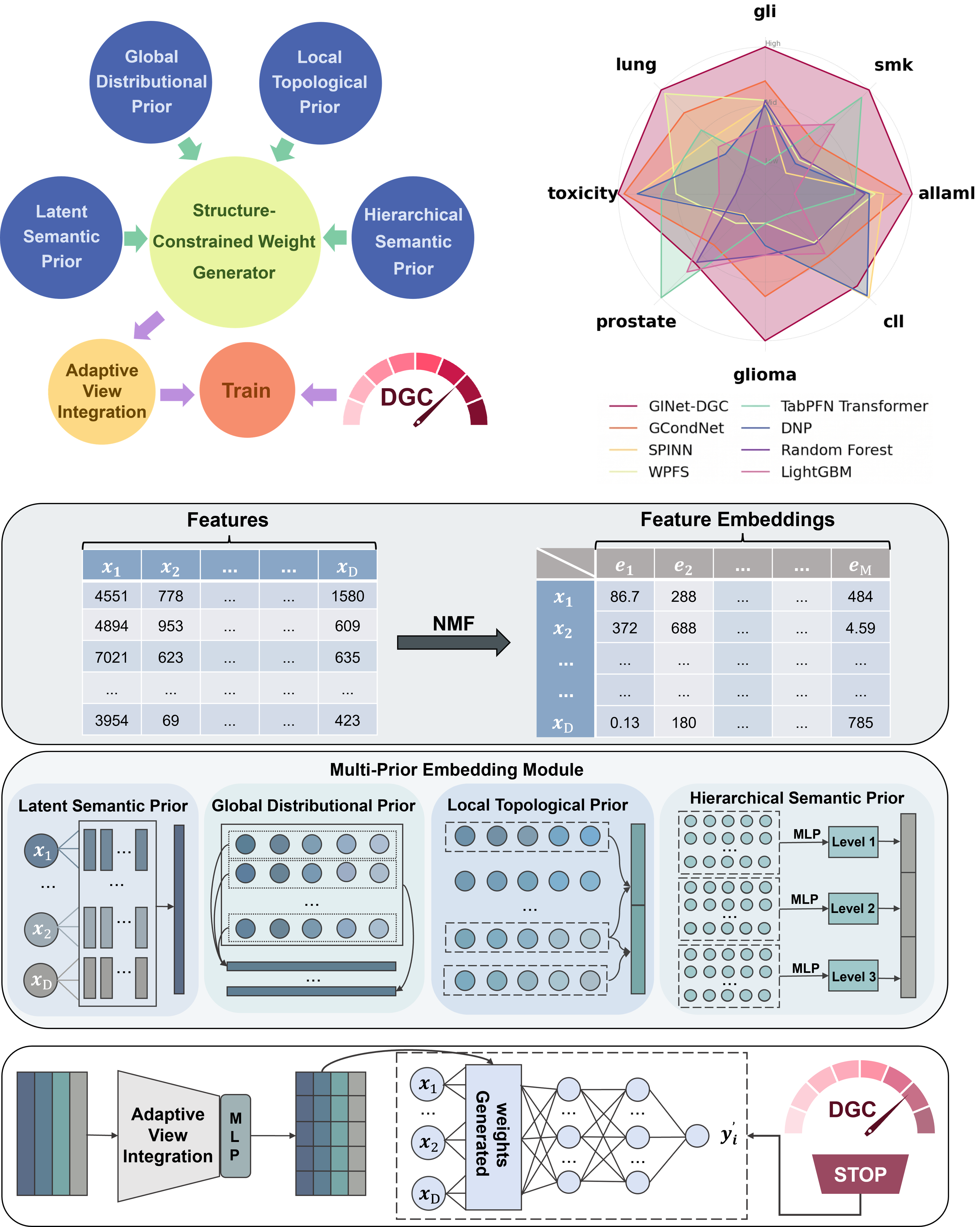
Therefore, we propose GINet-DGC, a neural framework engineered with structural inductive biases and adaptive trajectory-based early stopping. As illustrated in Figure 1, instead of fitting an unconstrained projection directly from scarce observations, GINet-DGC employs a Structure-Constrained Weight Generation Mechanism. This module synthesizes task-specific weights from multi-view feature embeddings to narrow the interaction search space. Simultaneously, the Dynamic Generalization Control strategy monitors the training trajectory via an Overfitting-aware Index (OFI) to determine adaptive termination. As shown in Figure 2, performance comparisons across multiple benchmarks demonstrate that GINet-DGC achieves competitive and relatively stable results.
1.4. Main Contributions
The main contributions of this research are summarized as follows:
- Framework Proposal: We introduce GINet-DGC, an end-to-end framework tailored with structural inductive biases to resolve the strict sample constraints in biomedical HDLSS tasks.
- Weight Generation Mechanism: We develop a structure-constrained generator that fuses multi-view statistical, topological, and sparse priors to model high-dimensional gene-expression features robustly.
- Adaptive Early Stopping: We implement an Overfitting-aware Index (OFI) alongside an adaptive training strategy to monitor generalization behavior and prevent overfitting during optimization.
- Extensive Empirical Validation: We comprehensively evaluate the proposed framework on eight public gene-expression datasets using repeated stratified cross-validation against 17 baseline models, demonstrating competitive stability.
2. Materials and Methods
The proposed GINet-DGC framework addresses the challenge of learning from biomedical high-dimensional, low-sample-size data. In these scenarios, molecular features greatly outnumber available clinical observations, meaning that increasing model depth blindly risks severe overfitting. Therefore, our approach introduces structural inductive biases to constrain the parameter solution space. We propose a unified framework that integrates a Structure-Constrained Weight Generator and a Dynamic Generalization Control adaptive stopping strategy. The source code for replication is publicly available at: https://github.com/user123h/Global_Interaction.
Figure 3 outlines the complete methodological workflow of this research, and Section 2.1, Section 2.2, Section 2.3, Section 2.4, and Section 2.5 provide detailed descriptions of the proposed framework, training process, and experimental protocol.
2.1. Model Overview
The framework consists of two core components: the Structure-Constrained Weight Generator, which integrates multi-view structural priors from high-dimensional biomedical features and synthesizes adaptive weight representations; Dynamic Generalization Control, an adaptive early stopping strategy that monitors the training trajectory under some constraints. Figure 3 outlines the overall workflow of the proposed GINet-DGC framework.
2.2. Structure-Constrained Weight Generator
In high-dimensional low-sample-size settings, directly optimizing the first-layer feature interaction matrix as an unconstrained parameter block often results in severe over-parameterization. Prior studies have shown that structured parameter generation and conditional weight prediction can effectively improve generalization by reducing the freedom of model parameters. Inspired by this idea, GINet-DGC introduces multi-view feature-level structural priors to condition the construction of the input interaction matrix. Conceptually, this mechanism resembles a structurally constrained HyperNetwork, as the interaction weights are generated under the guidance of feature descriptors rather than being freely optimized from limited training samples. By incorporating descriptor-based constraints into parameter generation, the proposed design reduces the effective search space of the optimization process and alleviates parameter redundancy, thereby improving robustness in HDLSS scenarios.
We use the following notation throughout this section. Let denote the original input matrix. Before applying non-negative matrix factorization (NMF), invalid samples are removed. The remaining expression values are then normalized by Min–Max Scaling so that each feature is linearly mapped into the interval :
where the minimum and maximum are computed over samples for each feature. The resulting preprocessed matrix is denoted as , with N valid samples and D features, and M denotes the feature-embedding dimension. GINet-DGC then applies NMF directly to decompose the preprocessed non-negative matrix X:
where U captures the latent sample-specific configurations, and represents the feature-wise semantic matrix. The rows of V, denoted as , are extracted directly as the stable latent semantic embeddings for each of the D high-dimensional features. In HDLSS data, this non-negativity constraint encourages additive, part-based feature semantics can prevents arbitrary cancellation among noisy variables. Consequently, the rows of V yield stable local semantic bases, which are inherently easier to regularize than a dense global mapping [29]. Prior work demonstrates that such feature-wise embeddings V significantly improve conditional weight prediction in high-dimensional tabular learning [20].
The objective of the Structure-Constrained Weight Generator is to synthesize the first-layer projection matrix A from the structural priors extracted from V. The generation process is defined as
where H denotes the hidden width of the first classifier layer, the generator parameters are denoted by , and denotes the fused multi-view structural representation. The generated matrix A is subsequently utilized by the task classifier , whose remaining trainable parameters are denoted by .
GINet-DGC extracts structural priors from four complementary views:
- 1.
- Latent Semantic Prior: It constructs basic subspace constraints.
- 2.
- Global Distributional Prior: It captures dataset-wide statistical stability.
- 3.
- Local Topological Prior: It preserves manifold geometry among features.
- 4.
- Hierarchical Semantic Prior: It provides multi-scale nonlinear abstractions.
Then an adaptive integration mechanism fuses these multi-view priors to form a structure-constrained representation. The generation process is summarized as follows:
Here, , , , and denote the four prior extraction modules. The generated matrix A strictly constrains the classifier’s first-layer search space. Independently, the Dynamic Generalization Control strategy monitors the training trajectory and terminates optimization when the validation behavior indicates generalization saturation.
2.2.1. Latent Semantic Prior
The Latent Semantic Prior module transforms the feature matrix into a compact subspace representation. Its primary role is to impose a localized structural constraint. For each feature embedding vector (where ), the nonlinear mapping is defined as
where is the nonlinear activation function, while and denote the learnable weight matrix and bias vector of this module, respectively. The complete latent representation for all features is stacked as . This projection filters out redundant coordinate noise and maps feature-wise behaviors into a smooth, compact latent semantic space.
2.2.2. Global Distributional Prior
The Global Distributional Prior module captures the macroscopic statistical regularities of the feature-embedding space. Utilizing the embedding matrix , the module flattens all subspace variables to compute a global descriptor vector :
Here, the vector elements denote the global mean, median, standard deviation, variance, skewness, kurtosis, range, and interquartile range of the flattened matrix V. To calibrate the importance of different statistical properties, a learnable weight vector is introduced via element-wise multiplication.
The weighted statistical vector is expanded along the feature dimension D to construct an extended prior matrix . This matrix is mapped through two linear projection layers to extract cross-descriptor interactions:
where . The matrix is broadcasted from , and ⊙ denotes the Hadamard product. This layout restricts the classifier’s search space based on dataset-wide regularities.
2.2.3. Local Topological Prior
The Local Topological Prior module models the neighborhood geometry and manifold patterns within the latent subspace [30]. It extracts structural descriptors from V via a joint soft-clustering and K-nearest neighbor formulation.
The module maintains learnable cluster centers . For each feature vector , the soft assignment to center is defined as
where is a learnable temperature, and is the j-th element of the cluster scaling vector . Concurrently, the module extracts local density by computing Euclidean distances to the nearest neighbors:
The soft-clustering assignments and KNN distance profiles jointly form the topological descriptor , capturing both coarse cluster affinity and local neighborhood geometry. The final prior is generated via a linear projection layer:
where and are learnable weights and biases.
2.2.4. Hierarchical Semantic Prior
To capture dependencies across semantic scales, this module employs L parallel shallow subnetworks, each projecting the embedding matrix V into a scale-specific representation:
where and represent level-specific parameters. All branch outputs are concatenated into a joint tensor . The hierarchical prior is synthesized via a final fusion layer:
where and denote the learnable fusion weights and biases.
2.2.5. Adaptive Prior Integration and Weight Generation
The integration layer models the non-linear interactions across the multi-view descriptors. The structural prior fields are concatenated to form a unified tensor . To adjust feature-wise contributions dynamically, a multi-head self-attention mechanism [31] maps the contextual dependencies:
where are learnable projection weights. This Transformer-based layout enhances global dependency modeling and representational flexibility.
Finally, the weight generator maps the fused representation to synthesize the target task projection matrix A:
where represent the sequential linear layers, and the transpose operator ensures that the spatial dimensions of A match the first classifier layer exactly.
2.3. Dynamic Generalization Control
In HDLSS tasks, overfitting is not only a final-state problem but also a trajectory problem: the model may continue reducing training loss after validation performance has saturated or begun to deteriorate. Therefore, rather than relying on standard fixed stopping rules [32,33], we introduce an adaptive early stopping strategy termed Dynamic Generalization Control. DGC closely tracks the training trajectory to determine if the optimization process has entered an overfitting regime, where subsequent parameter updates serve primarily to widen the generalization gap.
The stopping signal is the Overfitting-aware Index, which integrates three factors: accuracy discrepancy, loss discrepancy, and validation-performance deterioration. At iteration t, it is defined as
where denotes the validation deterioration trend over a recent window of iterations. A low deterioration trend reduces the overfitting warning, whereas a larger deterioration trend increases the warning when it co-occurs with growing train–validation gaps.
To avoid a manually fixed stopping threshold, DGC computes an adaptive threshold from the historical OFI distribution:
where and are the mean and standard deviation of previous OFI values, and controls threshold tolerance. Training is terminated only when for P consecutive validation checks. The OFI-related hyperparameters, including , , , , and P, are determined by automatic hyperparameter optimization rather than manual assignment. This patience-based decision separates the trajectory metric from the stopping rule and reduces sensitivity to transient validation fluctuations.
2.4. Training Process
The training objective is to minimize the cross-entropy loss between predictions and true labels:
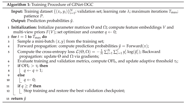
where is the true label indicator and represents the predicted probability. The training procedure is summarized in Algorithm 1.
2.5. Experimental Setup
2.5.1. Experimental Data
We evaluated the proposed framework on eight public high-dimensional low-sample size biomedical gene-expression datasets, spanning 50 to 203 samples and 3,312 to 22,283 features. Detailed dataset information is provided in Appendix A.
To ensure reproducibility, we performed repeated stratified 5-fold cross-validation with five independent repeats. Feature embeddings were generated independently within each training fold of the repeated stratified 5-fold cross-validation procedure. For each run, 80% of the data was allocated for development and 20% for testing. Within the development split, 10% of the samples were reserved as a validation subset for hyperparameter tuning and Dynamic Generalization Control. We report the mean balanced accuracy over all 25 test evaluations as the final performance metric.
2.5.2. Evaluation Metrics
We adopt Balanced Accuracy as the primary evaluation metric. Unlike traditional accuracy, balanced accuracy objectively reflects classification capability under class imbalance and small-sample conditions. In high-dimensional datasets, class distribution is often skewed. Standard accuracy can be misleading, as models may bias toward the majority class, obscuring their ability to recognize minority samples.
Balanced accuracy measures performance by averaging the recall of each class:
where C denotes the number of classes, and and represent true positives and false negatives for class c.
This metric provides a stable reflection of discriminative ability, especially in cases of severe imbalance or limited sample size.
2.5.3. GINet-DGC Settings
The classification backbone of GINet-DGC consists of three fully connected layers. The final layer uses Softmax for class distribution. The Structure-Constrained Weight Generator includes four prior extraction modules: a statistical feature extractor(64-dim output), a low-dimensional semantic encoder(64-dim output), a topological clustering module (32-dim output, 8 centers), and a multi-level feature module (64-dim output). The adaptive attention mechanism outputs 128-dimensional fused features. Finally, the generator produces 100-dimensional weights.
For the Dynamic Generalization Control adaptive stopping strategy, the OFI-related hyperparameters were obtained through automatic hyperparameter optimization on the validation subset. The selected trajectory weights in the reported experiments were (accuracy gap), (loss gap), and (validation deterioration trend), with threshold tolerance and patience parameters selected by the same validation-search procedure. We employ Batch Normalization [34] and Dropout [35]. LeakyReLU is used for activation to improve stability.
The model is trained using AdamW [36] with a batch size of 8. The maximum training steps are set to 5000.
3. Results
3.1. Baselines
We compare GINet-DGC against 17 representative baselines. These cover traditional machine learning, modern neural architectures, and specialized HDLSS approaches. For fairness, all baseline methods are evaluated on the same eight public datasets and under the same repeated stratified 5×5 cross-validation protocol, and the reported balanced accuracy is averaged over the resulting 25 evaluations. We do not directly copy performance numbers from prior publications when their datasets, generated samples, preprocessing pipelines, or split protocols are not fully aligned with ours.
For traditional methods, we selected Random Forest [37] and LightGBM [11]. These represent bagging and gradient boosting frameworks. They are known for robustness on sparse data.
For deep tabular models, we include standard MLP, TabNet [13], TabTransformer [14], LassoNet [38], DNP [39], and Hypertab [18]. We also include TabPFN [26], a recent foundation model for tabular learning. TabPFN leverages Bayesian priors and conditional sampling, representing a strong small-sample tabular baseline.
For feature generation and structured learning, we evaluate DietNetworks [19], FsNet [16], SPINN [40], and WPFS [20]. We also evaluate GCondNet [21], GCN [41], and GATv2 [42]. These methods enhance representation through mechanisms like conditional weight prediction and implicit relational modeling.
3.2. Benchmark Comparison
Table 1 summarizes the mean balanced accuracy of all evaluated methods across the eight biomedical HDLSS datasets under repeated stratified 5×5 cross-validation.
As shown in Table 1, GINet-DGC demonstrates competitive performance across eight high-dimensional small-sample biomedical datasets. This supports the usefulness of its structural modeling and adaptive stopping strategy for bioinformatics prediction benchmarks. Specifically, GINet-DGC ranks among the top three on all datasets and achieves the highest balanced accuracy on gli, smk, allaml, glioma, toxicity, and lung. Its average rank is 1.50, lower than other recent competitive models such as GCondNet (3.00) and TabPFNTransformer (5.88). This indicates relatively stable performance across the evaluated public biomedical benchmarks.
Regarding model categories, traditional tree-based models remain competitive in certain biomedical tasks. They benefit from robustness to low-order statistics. However, they often underperform compared to deep modeling methods. This is because tree models rely on local greedy partitioning. They struggle to capture global dependencies among high-dimensional molecular variables. This restricts their representation power.
Deep tabular models generally perform stably. Models like DNP and TabPFN show strong generalization. However, they rely on complex priors or pretraining. This may increase sensitivity to distribution shifts between biomedical cohorts or assay conditions. Notably, GINet-DGC achieves competitive performance without external pretraining.
Among feature generation methods, SPINN and GCondNet achieve strong results. This demonstrates the value of explicit relation modeling. However, they rely on strong local assumptions. This makes them sensitive to noise. In contrast, our method models high-order interactions globally while preserving local constraints. This enhances robustness under complex biomedical feature distributions.
Overall, GINet-DGC maintains competitive performance in the evaluated biomedical HDLSS conditions. This supports the usefulness of its structured global interaction design and adaptive early stopping strategy for data-scarce bioinformatics prediction tasks.
3.3. Ablation Study
3.3.1. Multi-View Structural Priors
To quantify the contribution of each prior branch, we conducted an ablation study by systematically removing individual modules. Figure 4 summarizes the resulting performance variations.
The performance degradation exhibits clear task-dependent patterns, reflecting the structural heterogeneity inherent in HDLSS data. Specifically, isolating or removing the hierarchical semantic or local topological prior yields the most pronounced performance drops across the majority of tasks. This confirms that different datasets rely on distinct dominant geometric or categorical regularities. Rather than displaying uniform dominance, the multi-view descriptors offer complementary structural constraints. These findings validate the necessity of our adaptive fusion layer, which dynamically calibrates multi-view representations instead of assuming static, equal contributions across tasks.
3.3.2. Adaptive Prior Integration
To evaluate the attention module, we conducted an ablation by removing it while keeping all feature layers. Figure 5 reports the comparison between the full model and the variant without attention. As shown in Figure 5, the attention mechanism contributes to performance. Removing it leads to a noticeable drop, with the most pronounced decline on the glioma dataset ( decrease). This indicates that attention enables adaptive weighting. It strengthens important channels and suppresses redundancy. This enhances feature fusion.
We also investigated the dependency on multi-view features via a “J-Attention” experiment (attention only, no structural priors). Figure 6 presents the comparison between this attention-only variant and the full GINet-DGC model. As shown in Figure 6, J-Attention performs worse than the full model in the evaluated setting. This indicates that attention alone is limited. It requires structured multi-level features to be effective. Consequently, it fails to capture implicit structures in high-dimensional data without them. Therefore, the attention module operates synergistically with the multi-layer embedding. It is not an isolated factor.
In summary, the structured weight generation strategy improves stability in the evaluated settings. We conducted further comparisons with other initialization strategies (Appendix B), which further support the usefulness of the proposed structure-constrained generation mechanism.
3.4. Analysis of Dynamic Generalization Control
To verify the DGC adaptive stopping strategy, we compared models with and without it on eight datasets. Figure 7 summarizes the effect of DGC on both predictive performance and convergence behavior. As shown in Figure 7, DGC-equipped models achieve an average improvement of ~1% on complex datasets (e.g., smk, glioma). They also reduce convergence steps in some cases (e.g., from 2575 to 1587 in glioma). This indicates that the adaptive OFI threshold can replace fixed early stopping. It allows the stopping decision to adjust based on training dynamics. This avoids underfitting and reduces over-iteration. In summary, DGC enhances generalization and improves efficiency. This validates the practical value of the adaptive early stopping strategy. Applying this mechanism to GCondNet (Appendix B) also yielded gains, demonstrating transferability.
3.5. Training Dynamics
Figure 8 compares the training processes of GINet-DGC and MLP. GINet-DGC exhibits brief early oscillation, followed by rapid stabilization. It maintains higher validation accuracy and lower loss throughout. According to literature [43], early oscillations relate to adaptive parameter adjustment. The network aligns effective feature directions under small-scale initialization. Overall, GINet-DGC demonstrates faster convergence and greater stability than MLP in this example, supporting its robustness in high-dimensional, small-sample biomedical prediction tasks.
4. Discussion
The empirical results demonstrate that GINet-DGC effectively addresses the fundamental challenges of High-Dimensional Low-Sample Size (HDLSS) learning by combining structure-constrained weight generation with adaptive generalization monitoring. Rather than relying on external pretraining or data augmentation, our framework leverages feature-wise structural priors to provide robust mathematical constraints. This methodology successfully regularizes the classification search space when sample sizes are heavily restricted and features are highly redundant.
A key structural finding from the ablation study is that individual prior branches exhibit task-dependent importance, reflecting the distinct geometric or categorical regularities inherent in heterogeneous tabular data. This underscores the necessity of our adaptive fusion layer, which dynamically calibrates multi-view representations instead of assuming static, uniform contributions.
Crucially, the underlying weight generation and trajectory monitoring mechanisms in GINet-DGC hold the potential to extend to broader tabular tasks. The framework could be adapted to other scenarios characterized by high-dimensional, small-sample constraints, ranging from clinical biomarker identification to specific prediction tasks in alternative scientific domains.
Future research will expand in three strategic directions: (1) investigating the direct biological interpretation and visualization of the generated projection weights to map downstream molecular patterns; (2) validating the framework’s scalability on significantly larger, diverse tabular datasets to test its broader generalization limits; and (3) OFI is composed of multiple metric terms whose weighting coefficients are currently determined mainly through validation-based search,future work could explore a dynamic balancing mechanism that adjusts the relative contributions of OFI components during training, rather than relying only on fixed hyperparameters or conventional parameter-search procedures.
5. Conclusions
In this study, we proposed GINet-DGC to address the optimization and over-iteration challenges in High-Dimensional Low-Sample Size learning. By using a Structure-Constrained Weight Generator to synthesize projection weights from multi-view structural priors, the framework effectively restricts the feature-interaction search space under limited supervision. Concurrently, the Overfitting-aware Index enables adaptive training termination before performance saturates. Extensive evaluations across eight typical biomedical datasets demonstrate that our method achieves competitive classification performance and relatively stable generalization behavior. These findings support GINet-DGC as a viable and structurally constrained modeling strategy for data-scarce bioinformatics benchmarks.
Author Contributions
Conceptualization, Xinran Zhang; methodology, Xinran Zhang; investigation, Xinran Zhang; writing—original draft preparation, Xinran Zhang; methodological guidance, comparative experiment solving, and experimental recording, Yang Sheng; comparative experiments and experimental-result recording, Sijie Shen; data collection, manuscript revision, and content review, Dongjie Fan; supervision, experimental guidance, and manuscript-writing guidance, Lizhuang Liu. All authors have read and agreed to the published version of the manuscript.
Funding
This work was supported by Grant No. E1421H1E01.
Institutional Review Board Statement
Not applicable.
Informed Consent Statement
Not applicable.
Data Availability Statement
The datasets used in this study are publicly available benchmarks described in Section 2.5.1 and Appendix A. No new datasets were generated. The source code for replication is available at https://github.com/user123h/Global_Interaction.
Acknowledgments
During the preparation of this work, the authors used ChatGPT to improve the language quality and clarity of the manuscript. After using this tool, the authors reviewed and edited the content as needed and take full responsibility for the content of the publication.
Conflicts of Interest
The authors declare no conflicts of interest.
Abbreviations
| AI | Artificial Intelligence |
| BA | Balanced Accuracy |
| DGC | Dynamic Generalization Control |
| DNN | Deep Neural Network |
| HDLSS | High-Dimensional Low-Sample Size |
| NMF | Non-negative Matrix Factorization |
| OFI | Overfitting-aware Index |
| SCWG | Structure-Constrained Weight Generator |
Appendix A. Detailed Dataset Description
To support reproducibility, this appendix reports the sample size and feature dimensionality of the eight public biomedical gene-expression datasets used in this study. All datasets originate from publicly available bioinformatics benchmark studies [21], and their standardized versions can be obtained from online repositories.
These datasets are widely used in biomedical benchmarking for gene-expression pattern recognition, cancer type diagnosis support, and drug-toxicity prediction. They are characterized by limited sample sizes and extremely high feature dimensionality, making them representative HDLSS benchmarks. The detailed dataset statistics are summarized in Table A1.

Table A1.
Summary of datasets used in this study.
| Name | Size | Features |
|---|---|---|
| Allaml | 72 | 7129 |
| CLL | 111 | 11340 |
| Gli | 85 | 22283 |
| Glioma | 50 | 4434 |
| Lung | 203 | 3312 |
| Prostate | 102 | 5966 |
| Smk | 187 | 19993 |
| Toxicity | 171 | 5748 |
The dataset selection follows a reproducibility-oriented criterion. We only include real-world datasets whose feature matrices and labels are publicly accessible and can be independently reconstructed without relying on author-generated samples, private preprocessing artifacts, or non-public data augmentation.
Appendix B. Explanation of Ablation Effectiveness
To evaluate the robustness of the proposed model against parameter initialization sensitivity, we compared four commonly used initialization methods (Kaiming, NMF, PCA, and Xavier) with the proposed Structure-Constrained Weight Generator (SCWG) of GINet-DGC. For fair comparison, all baselines were trained under identical configurations, including consistent optimization hyperparameters and the same DGC adaptive stopping strategy. The balanced accuracy results on eight HDLSS datasets are presented in Table B1.
Experimental results demonstrate that GINet-DGC achieves competitive performance compared with conventional initialization strategies. This indicates that the model’s structural priors effectively constrain the solution space, mitigating sensitivity to random initialization and ensuring stable convergence. In contrast, general-purpose methods like Kaiming and Xavier show instability in specific tasks, while simple matrix decomposition lacks sufficient expressiveness. Overall, the SCWG mechanism demonstrates robustness akin to a regularization prior, supporting its reliability in data-scarce regimes.
Table B1.
Performance comparison against initialization strategies on eight datasets.
| Initialization | Gli | Smk | Allaml | CLL | Glioma | Prostate | Toxicity | Lung |
|---|---|---|---|---|---|---|---|---|
| Kaiming | 83.45 | 70.78 | 88.06 | 73.32 | 65.50 | 90.47 | 83.51 | 95.20 |
| NMF | 82.43 | 66.14 | 90.15 | 70.50 | 64.67 | 88.67 | 84.71 | 95.20 |
| PCA | 79.53 | 60.66 | 93.78 | 77.91 | 63.83 | 89.27 | 93.97 | 95.95 |
| Xavier | 87.33 | 70.67 | 93.78 | 81.47 | 63.83 | 92.27 | 83.75 | 96.88 |
| GINet-DGC | 90.80 | 72.06 | 98.00 | 84.02 | 79.99 | 91.43 | 96.04 | 98.77 |
Note. Comparison of balanced accuracy (%) under different initialization strategies. GINet-DGC achieves favorable overall performance in this comparison, supporting the usefulness of its structure-constrained weight generation mechanism.
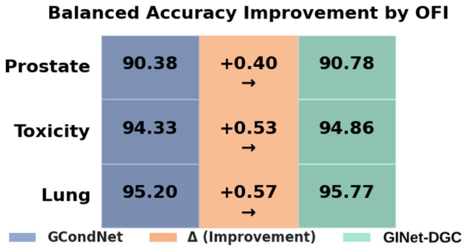
To verify the universality and transferability of the proposed Dynamic Generalization Control (DGC) strategy, we integrated this module into the GCondNet framework and conducted comparative experiments on the Prostate, Toxicity, and Lung datasets. Figure B1 illustrates the balanced accuracy improvements of the baseline GCondNet and GCondNet equipped with DGC. Results demonstrate that, under identical configurations, the incorporation of the DGC adaptive stopping strategy yields consistent enhancements, with an average improvement of approximately 0.50%. These findings confirm the effectiveness of the DGC strategy across different architectures, demonstrating its ability to alleviate overfitting through adaptive early stopping without altering the backbone structure. Figure B1 summarizes the balanced accuracy improvement obtained by integrating DGC into GCondNet across the evaluated datasets.
Figure B1.
Balanced accuracy improvement of GCondNet. After integrating the DGC strategy across multiple datasets. The DGC strategy adaptively determines the training horizon based on the OFI metric, enhancing generalization.
Figure B1.
Balanced accuracy improvement of GCondNet. After integrating the DGC strategy across multiple datasets. The DGC strategy adaptively determines the training horizon based on the OFI metric, enhancing generalization.
References
- Baldi, P.; Sadowski, P.; Whiteson, D. Searching for Exotic Particles in High-Energy Physics with Deep Learning. Nat. Commun. 2014, 5, 4308. [Google Scholar] [CrossRef]
- Keith, J.A.; Vassilev-Galindo, V.; Cheng, B.; Chmiela, S.; Gastegger, M.; Müller, K.R.; Tkatchenko, A. Combining Machine Learning and Computational Chemistry for Predictive Insights into Chemical Systems. Chem. Rev. 2021, 121, 9816–9872. [Google Scholar] [CrossRef] [PubMed]
- Feng, F.; He, X.; Wang, X.; Luo, C.; Liu, Y.; Chua, T.S. Temporal Relational Ranking for Stock Prediction. ACM Trans. Inf. Syst. 2019, 37, 1–30. [Google Scholar] [CrossRef]
- Wang, Z.; Gao, C.; Xiao, C.; Sun, J. MediTab: Scaling Medical Tabular Data Predictors via Data Consolidation, Enrichment, and Refinement. arXiv 2024, 2305.12081. [Google Scholar] [CrossRef]
- Ruan, Y.; Lan, X.; Tan, D.J.; Abdullah, H.R.; Feng, M. P-Transformer: A Prompt-Based Multimodal Transformer Architecture for Medical Tabular Data. arXiv 2025, 2303.17408. [Google Scholar] [CrossRef]
- Golling, T.; Heinrich, L.; Kagan, M.; Klein, S.; Leigh, M.; Osadchy, M.; Raine, J.A. Masked Particle Modeling on Sets: Towards Self-Supervised High Energy Physics Foundation Models. arXiv 2024, 2401.13537. [Google Scholar] [CrossRef]
- Zou, J.; Huss, M.; Abid, A.; Mohammadi, P.; Torkamani, A.; Telenti, A. A Primer on Deep Learning in Genomics. Nat. Genet. 2019, 51, 12–18. [Google Scholar] [CrossRef]
- Shwartz-Ziv, R.; Armon, A. Tabular Data: Deep Learning Is Not All You Need. arXiv 2021, 2106.03253. [Google Scholar] [CrossRef]
- Gorishniy, Y.; Rubachev, I.; Khrulkov, V.; Babenko, A. Revisiting Deep Learning Models for Tabular Data. Adv. Neural Inf. Process. Syst. 2021, 34, 18932–18943. [Google Scholar]
- Chen, T.; Guestrin, C. XGBoost: A Scalable Tree Boosting System. In Proceedings of the Proceedings of the 22nd ACM SIGKDD International Conference on Knowledge Discovery and Data Mining, 2016; pp. 785–794. [Google Scholar] [CrossRef]
- Ke, G.; Meng, Q.; Finley, T.; Wang, T.; Chen, W.; Ma, W.; Ye, Q.; Liu, T.Y. LightGBM: A Highly Efficient Gradient Boosting Decision Tree. In Proceedings of the Advances in Neural Information Processing Systems, 2017. [Google Scholar]
- Song, W.; Shi, C.; Xiao, Z.; Duan, Z.; Tang, J.; Xu, Y.; Zhang, M. AutoInt: Automatic Feature Interaction Learning via Self-Attentive Neural Networks. In Proceedings of the Proceedings of the 28th ACM International Conference on Information and Knowledge Management, 2019; pp. 1161–1170. [Google Scholar] [CrossRef]
- Arik, S.O.; Pfister, T. TabNet: Attentive Interpretable Tabular Learning. Proc. AAAI Conf. Artif. Intell. 2021, 35, 6679–6687. [Google Scholar] [CrossRef]
- Huang, X.; Khetan, A.; Cvitkovic, M.; Karnin, Z. TabTransformer: Tabular Data Modeling Using Contextual Embeddings. arXiv 2020, 2012.06678. [Google Scholar] [CrossRef]
- Somepalli, G.; Goldblum, M.; Schwarzschild, A.; Bruss, C.B.; Goldstein, T. SAINT: Improved Neural Networks for Tabular Data via Row Attention and Contrastive Pre-Training. arXiv 2021, 2106.01342. [Google Scholar] [CrossRef]
- Singh, D.; Yamada, M. FsNet: Feature Selection Network on High-Dimensional Biological Data; Manuscript, 2020. [Google Scholar]
- Ha, D.; Dai, A.; Le, Q.V. HyperNetworks. In Proceedings of the International Conference on Learning Representations, 2017. [Google Scholar]
- Wydmanski, W.; Bulenok, V. HyperTab: Hypernetwork Approach for Deep Learning on Small Tabular Datasets. arXiv 2023, 2303.00923. [Google Scholar] [CrossRef]
- Romero, A.; Carrier, P.L.; Erraqabi, A.; Sylvain, T.; Auvolat, A.; Dejoie, E.; Legault, M.A.; Dubé, M.P.; Hussin, J.G.; Bengio, Y. Diet Networks: Thin Parameters for Fat Genomics. In Proceedings of the International Conference on Learning Representations, 2017. [Google Scholar]
- Margeloiu, A.; Simidjievski, N.; Liò, P.; Jamnik, M. Weight Predictor Network with Feature Selection for Small Sample Tabular Biomedical Data. arXiv 2022, 2211.15616. [Google Scholar] [CrossRef]
- Margeloiu, A.; Simidjievski, N.; Liò, P.; Jamnik, M. GCondNet: A Novel Method for Improving Neural Networks on Small High-Dimensional Tabular Data. arXiv 2024, 2211.06302. [Google Scholar] [CrossRef]
- Chawla, N.V.; Bowyer, K.W.; Hall, L.O.; Kegelmeyer, W.P. SMOTE: Synthetic Minority Over-Sampling Technique. J. Artif. Intell. Res. 2002, 16, 321–357. [Google Scholar] [CrossRef]
- He, H.; Bai, Y.; Garcia, E.A.; Li, S. ADASYN: Adaptive Synthetic Sampling Approach for Imbalanced Learning. In Proceedings of the IEEE International Joint Conference on Neural Networks, 2008; pp. 1322–1328. [Google Scholar] [CrossRef]
- Xu, L.; Skoularidou, M.; Cuesta-Infante, A.; Veeramachaneni, K. Modeling Tabular Data Using Conditional GAN. In Proceedings of the Advances in Neural Information Processing Systems, 2019. [Google Scholar]
- Kotelnikov, A.; Baranchuk, D.; Rubachev, I.; Babenko, A. TabDDPM: Modelling Tabular Data with Diffusion Models. In Proceedings of the International Conference on Machine Learning, 2023; pp. 17564–17579. [Google Scholar]
- Hollmann, N.; Müller, S.; Purucker, L.; Krishnakumar, A.; Körfer, M.; Hoo, S.B.; Schirrmeister, R.T.; Hutter, F. Accurate Predictions on Small Data with a Tabular Foundation Model. Nature 2025, 637, 319–326. [Google Scholar] [CrossRef]
- Gardner, J.; Perdomo, J.C.; Schmidt, L. Large Scale Transfer Learning for Tabular Data via Language Modeling. arXiv 2024, 2406.12031. [Google Scholar] [CrossRef]
- Liu, B.; Wei, Y.; Zhang, Y.; Yang, Q. Deep Neural Networks for High Dimension, Low Sample Size Data. In Proceedings of the Proceedings of the Twenty-Sixth International Joint Conference on Artificial Intelligence, 2017; pp. 2287–2293. [Google Scholar] [CrossRef]
- Lee, D.D.; Seung, H.S. Learning the Parts of Objects by Non-Negative Matrix Factorization. Nature 1999, 401, 788–791. [Google Scholar] [CrossRef] [PubMed]
- Xie, J.; Girshick, R.; Farhadi, A. Unsupervised Deep Embedding for Clustering Analysis. In Proceedings of the International Conference on Machine Learning, 2016; pp. 478–487. [Google Scholar]
- Vaswani, A.; Shazeer, N.; Parmar, N.; Uszkoreit, J.; Jones, L.; Gomez, A.N.; Kaiser, L.; Polosukhin, I. Attention Is All You Need. arXiv 2017, 1706.03762. [Google Scholar] [CrossRef]
- Prechelt, L. Early Stopping – But When? In Neural Networks: Tricks of the Trade; Springer, 1998; pp. 55–69. [Google Scholar] [CrossRef]
- LeCun, Y.; Bengio, Y.; Hinton, G. Deep Learning. Nature 2015, 521, 436–444. [Google Scholar] [CrossRef]
- Ioffe, S.; Szegedy, C. Batch Normalization: Accelerating Deep Network Training by Reducing Internal Covariate Shift. In Proceedings of the International Conference on Machine Learning, 2015; pp. 448–456. [Google Scholar]
- Srivastava, N.; Hinton, G.; Krizhevsky, A.; Sutskever, I.; Salakhutdinov, R. Dropout: A Simple Way to Prevent Neural Networks from Overfitting. J. Mach. Learn. Res. 2014, 15, 1929–1958. [Google Scholar]
- Loshchilov, I.; Hutter, F. Decoupled Weight Decay Regularization. In Proceedings of the International Conference on Learning Representations, 2019. [Google Scholar]
- Breiman, L. Random Forests. Mach. Learn. 2001, 45, 5–32. [Google Scholar] [CrossRef]
- Lemhadri, I.; Ruan, F.; Abraham, L.; Tibshirani, R. LassoNet: A Neural Network with Feature Sparsity. arXiv 2021, 1907.12207. [Google Scholar] [CrossRef]
- Liu, B.; Wei, Y.; Zhang, Y.; Yang, Q. Deep Neural Networks for High Dimension, Low Sample Size Data. In Proceedings of the Proceedings of the Twenty-Sixth International Joint Conference on Artificial Intelligence, 2017; pp. 2287–2293. [Google Scholar] [CrossRef]
- Feng, J.; Simon, N. Sparse-Input Neural Networks for High-Dimensional Nonparametric Regression and Classification. arXiv 2019, 1711.07592. [Google Scholar] [CrossRef]
- Kipf, T.N.; Welling, M. Semi-Supervised Classification with Graph Convolutional Networks. In Proceedings of the International Conference on Learning Representations, 2017. [Google Scholar]
- Brody, S.; Alon, U.; Yahav, E. How Attentive Are Graph Attention Networks? arXiv 2022, 2105.14491. [Google Scholar] [CrossRef]
- Cohen, J.M.; Li, Y.; Zhang, Z. Early Training Dynamics and Oscillations in Neural Networks, 2024. Manuscript.
Figure 1.
Data flow of the GINet-DGC framework. Raw high-dimensional features are transformed into four feature-wise structural priors: latent semantic, global distributional, local topological, and hierarchical representations. These priors are adaptively fused to condition the Structure-Constrained Weight Generator, while Dynamic Generalization Control monitors the training trajectory through the Overfitting-aware Index and terminates optimization when generalization saturates.
Figure 1.
Data flow of the GINet-DGC framework. Raw high-dimensional features are transformed into four feature-wise structural priors: latent semantic, global distributional, local topological, and hierarchical representations. These priors are adaptively fused to condition the Structure-Constrained Weight Generator, while Dynamic Generalization Control monitors the training trajectory through the Overfitting-aware Index and terminates optimization when generalization saturates.
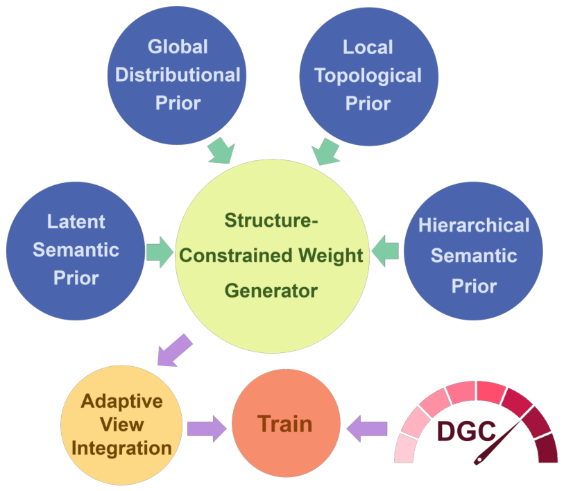
Figure 2.
Performance comparison of the top eight models ranked by balanced accuracy. The radar chart illustrates the normalized accuracy of the top eight models across multiple biomedical datasets. Overall, GINet-DGC demonstrates competitive performance across the evaluated datasets, indicating stable generalization under the considered biomedical HDLSS setting.
Figure 2.
Performance comparison of the top eight models ranked by balanced accuracy. The radar chart illustrates the normalized accuracy of the top eight models across multiple biomedical datasets. Overall, GINet-DGC demonstrates competitive performance across the evaluated datasets, indicating stable generalization under the considered biomedical HDLSS setting.
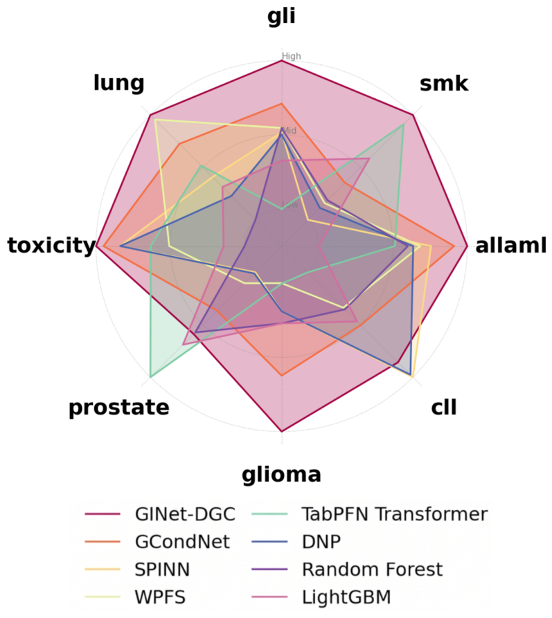
Figure 3.
Workflow of the GINet-DGC framework. The model first extracts Multi-View Structural Priors from high-dimensional biomedical features, including Latent Semantic, Global Distributional, Local Topological, and Hierarchical features. It then integrates these priors through Adaptive Constraint Integration to condition the Weight Generator and synthesize task-specific weights. Finally, Dynamic Generalization Control monitors the generalization trajectory and performs adaptive early stopping.
Figure 3.
Workflow of the GINet-DGC framework. The model first extracts Multi-View Structural Priors from high-dimensional biomedical features, including Latent Semantic, Global Distributional, Local Topological, and Hierarchical features. It then integrates these priors through Adaptive Constraint Integration to condition the Weight Generator and synthesize task-specific weights. Finally, Dynamic Generalization Control monitors the generalization trajectory and performs adaptive early stopping.
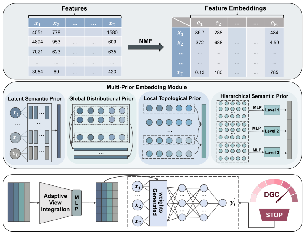
Figure 4.
Ablation results of the Structure-Constrained Weight Generator. Each curve represents performance after removing a specific prior branch: O-Low Level denotes removal of the latent semantic branch; O-Statistical Feature denotes removal of the global distributional prior; O-Clustering Feature denotes removal of the local topological prior; O-Multi-Level denotes removal of the hierarchical semantic prior. GINet-DGC represents the complete model. The full model achieves the best performance, confirming the effectiveness of structured weight generation.
Figure 4.
Ablation results of the Structure-Constrained Weight Generator. Each curve represents performance after removing a specific prior branch: O-Low Level denotes removal of the latent semantic branch; O-Statistical Feature denotes removal of the global distributional prior; O-Clustering Feature denotes removal of the local topological prior; O-Multi-Level denotes removal of the hierarchical semantic prior. GINet-DGC represents the complete model. The full model achieves the best performance, confirming the effectiveness of structured weight generation.
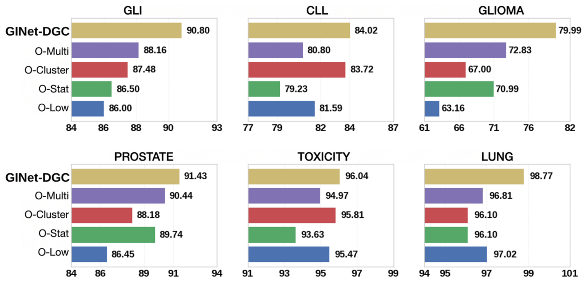
Figure 5.
Ablation results of the attention mechanism. Removing the attention module leads to a noticeable performance drop.
Figure 5.
Ablation results of the attention mechanism. Removing the attention module leads to a noticeable performance drop.
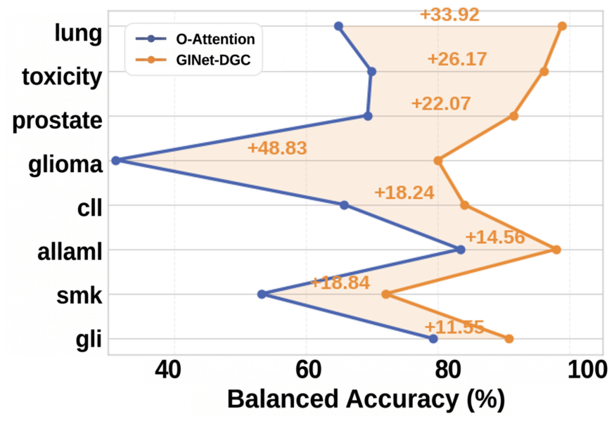
Figure 6.
Ablation results of the attention-only mechanism. The figure compares the attention-only model against the full GINet-DGC. The full model generally performs better than J-Attention, indicating that attention benefits from collaboration with structured priors.
Figure 6.
Ablation results of the attention-only mechanism. The figure compares the attention-only model against the full GINet-DGC. The full model generally performs better than J-Attention, indicating that attention benefits from collaboration with structured priors.
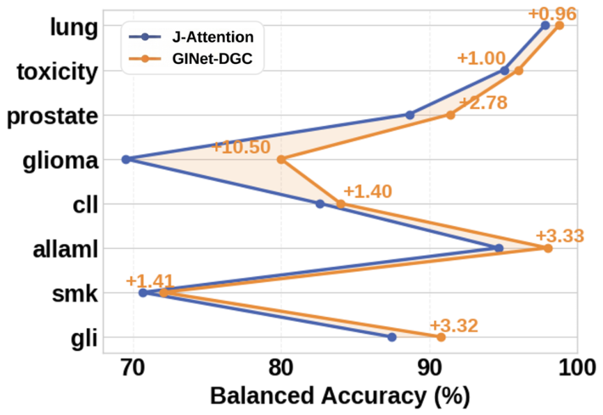
Figure 7.
Effect of DGC on generalization and convergence. The figure compares models with and without the DGC adaptive stopping strategy. DGC-equipped models achieve better performance (lines) and faster convergence (bars) in most tasks.
Figure 7.
Effect of DGC on generalization and convergence. The figure compares models with and without the DGC adaptive stopping strategy. DGC-equipped models achieve better performance (lines) and faster convergence (bars) in most tasks.
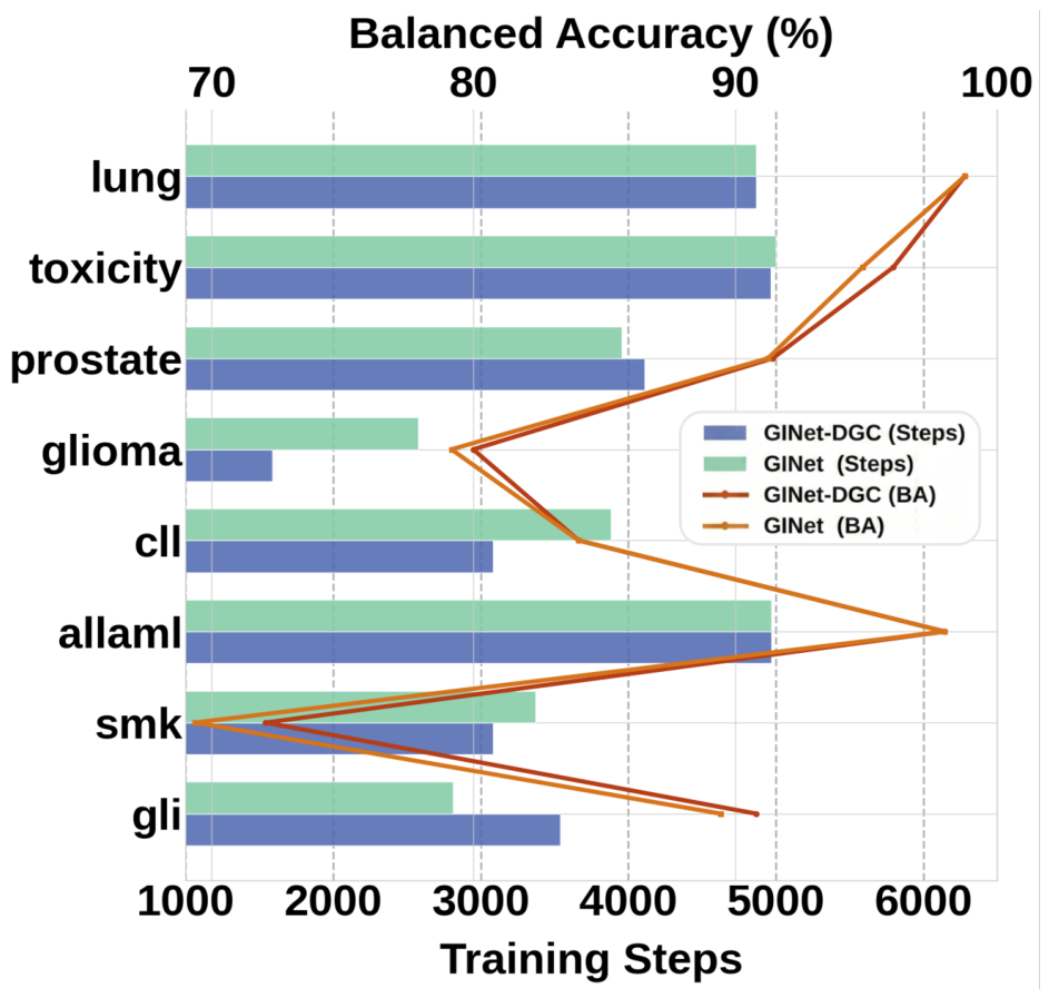
Figure 8.
Comparison of training dynamics (GINet-DGC vs. MLP) on the lung dataset. GINet-DGC experiences initial self-alignment oscillation, followed by rapid convergence. It identifies and halts the overfitting phase, indicating improved convergence efficiency and generalization retention.
Figure 8.
Comparison of training dynamics (GINet-DGC vs. MLP) on the lung dataset. GINet-DGC experiences initial self-alignment oscillation, followed by rapid convergence. It identifies and halts the overfitting phase, indicating improved convergence efficiency and generalization retention.
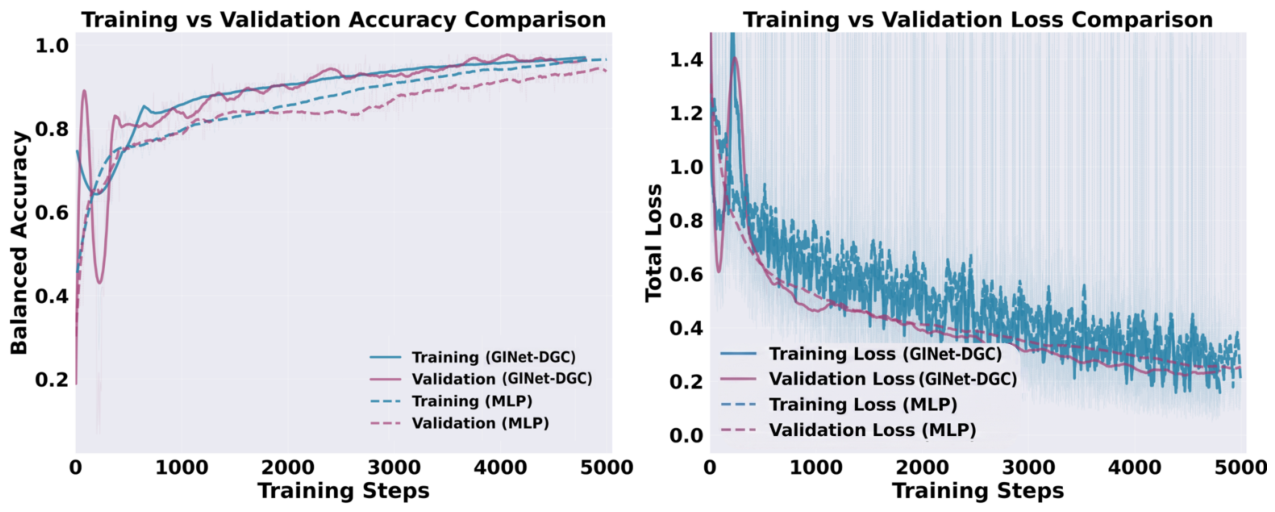
Table 1.
Mean balanced accuracy (%) across datasets under repeated stratified 5×5 cross-validation.
| Method | gli | smk | allaml | CLL | glioma | prostate | toxicity | lung | Avg-Rank |
|---|---|---|---|---|---|---|---|---|---|
| N/D | 0.004 | 0.009 | 0.01 | 0.01 | 0.011 | 0.017 | 0.03 | 0.059 | |
| DietNetworks | 76.42 | 62.71 | 92.00 | 68.84 | 68.00 | 81.71 | 82.13 | 90.43 | 11.50 |
| FsNet | 74.52 | 56.27 | 78.00 | 66.38 | 53.17 | 84.74 | 60.26 | 91.75 | 14.13 |
| DNP | 83.17 | 66.61 | 96.18 | 85.13 | 75.00 | 88.71 | 93.49 | 92.81 | 6.00 |
| SPINN | 83.39 | 65.91 | 96.78 | 85.35 | 75.00 | 88.66 | 93.50 | 94.20 | 4.25 |
| WPFS | 83.86 | 66.89 | 96.42 | 79.14 | 73.83 | 89.15 | 88.29 | 98.43 | 5.50 |
| TabNet | 64.49 | 61.16 | 69.66 | 50.87 | 45.99 | 65.48 | 41.59 | 70.92 | 15.13 |
| TabTransformer | 78.82 | 64.00 | 88.38 | 76.81 | 63.50 | 85.96 | 87.67 | 94.03 | 10.00 |
| Hypertab | 50.50 | 50.00 | 85.43 | 44.67 | 51.48 | 58.09 | 24.42 | 89.59 | 16.25 |
| CAE | 74.18 | 59.96 | 89.80 | 71.94 | 67.83 | 87.60 | 60.36 | 85.00 | 12.75 |
| LassoNet | 53.91 | 51.04 | 50.80 | 30.63 | 29.17 | 54.78 | 26.67 | 25.11 | 17.50 |
| MLP | 77.72 | 64.62 | 91.30 | 78.30 | 73.00 | 88.76 | 93.21 | 94.20 | 8.00 |
| Random Forest | 83.83 | 67.06 | 96.00 | 79.29 | 75.50 | 91.36 | 80.33 | 91.05 | 7.25 |
| LightGBM | 80.49 | 69.51 | 93.00 | 80.37 | 75.50 | 91.91 | 82.54 | 93.47 | 6.75 |
| GCN | 84.30 | 62.22 | 85.50 | 70.64 | 67.18 | 84.73 | 76.50 | 96.33 | 10.25 |
| GATv2 | 76.01 | 57.35 | 74.17 | 55.52 | 54.80 | 76.63 | 76.65 | 92.63 | 13.75 |
| GCondNet | 86.36 | 68.08 | 97.56 | 80.70 | 77.67 | 90.38 | 95.25 | 96.64 | 3.00 |
| TabPFNTransformer | 75.50 | 71.51 | 95.56 | 75.98 | 73.85 | 93.37 | 90.26 | 95.05 | 5.88 |
| GINet-DGC (ours) | 90.80 | 72.06 | 98.00 | 84.02 | 79.99 | 91.43 | 96.04 | 98.77 | 1.50 |
Note. Red, blue, and golden values indicate the best, second-best, and third-best performance on each dataset, respectively. All methods are evaluated on the same public datasets under the same repeated 5×5 cross-validation protocol.
Disclaimer/Publisher’s Note: The statements, opinions and data contained in all publications are solely those of the individual author(s) and contributor(s) and not of MDPI and/or the editor(s). MDPI and/or the editor(s) disclaim responsibility for any injury to people or property resulting from any ideas, methods, instructions or products referred to in the content. |
© 2026 by the authors. Licensee MDPI, Basel, Switzerland. This article is an open access article distributed under the terms and conditions of the Creative Commons Attribution (CC BY) license (http://creativecommons.org/licenses/by/4.0/).
Copyright: This open access article is published under a Creative Commons CC BY 4.0 license, which permit the free download, distribution, and reuse, provided that the author and preprint are cited in any reuse.


