

Submitted:
10 June 2026
Posted:
11 June 2026
You are already at the latest version
Abstract
Machine learning intrusion detection systems are routinely evaluated by randomly splitting a single dataset into training and test partitions and reporting accuracy or F1-score. This practice silently assumes that training and test traffic share one data-generating process, an assumption that fails whenever attacks, networks, or capture conditions change. This paper presents a controlled empirical study of concept drift in two widely used flow-based benchmarks, CSE-CIC-IDS2018 and CIC-DDoS2019, and shows that the evaluation protocol itself is the dominant variable governing reported performance. Under a random split, Random Forest, LightGBM, and a multilayer perceptron all reach macro-F1 ≈ 0.79–0.82 on CSE-CIC-IDS2018; under a class-blind chronological split the same models collapse to macro-F1 ≈ 0.02, a gap of 0.78 (95% bootstrap CI [0.75, 0.80], empirical p < 0.001). A label-shuffle control confirms the pipeline is leakage-free (macro-F1 0.065, at the 1/15 chance level). We further measure cross-dataset transfer from CSE-CIC-IDS2018 to two distinct CIC-DDoS2019 capture regimes: zero-shot transfer collapses in both (Matthews correlation coefficient −0.043 and −0.078, worse than chance). A small time-ordered target calibration buffer then repairs confidence reliably in both regimes (expected calibration error falling to ≤ 0.11 at the largest (10%) buffer) but restores discrimination unevenly, weakly in one regime (MCC to ≈ 0.26) and substantially in the other (MCC to ≈ 0.71), with the calibration metrics giving no indication of which outcome occurred. Repairing confidence therefore does not guarantee a usable model. A distributional analysis attributes the collapse to pervasive feature drift: 36 of 45 common-core features exceed the severe-drift threshold of PSI ≥ 0.25, with Kolmogorov–Smirnov statistics up to 0.79. We conclude that a credible intrusion-detection evaluation must report time-aware splits, cross-regime transfer, and calibration quality, not single-split accuracy.
Keywords:
concept drift
; intrusion detection
; evaluation methodology
; temporal bias
; calibration
; cross-dataset generalization
; CSE-CIC-IDS2018
; CIC-DDoS2019
1. Introduction
Machine learning intrusion detection systems (IDS) are usually evaluated by splitting a dataset into training and test portions, training a model, and reporting accuracy or F1-score. The approach is simple, but it assumes that the training and test data come from the same data-generating process. In cybersecurity this assumption is weak. Benign traffic changes with user behaviour, protocols, and services; attack traffic changes with adversary goals, tooling, and target surfaces; and the data pipeline itself changes when feature extractors or preprocessing scripts are replaced. These changes produce concept drift in a broad operational sense, and they determine whether a model that scores well in the laboratory will remain reliable after deployment. We use concept drift throughout in this broad sense, covering covariate shift, prior-probability shift, and the open-set arrival of previously unseen attack classes, rather than only the strict definition of a changing feature-label mapping. Where the distinction matters we are explicit: the within-dataset collapse we report (Section 6.1) is an open-set, unseen-class phenomenon, whereas the cross-dataset collapse (Section 6.2 and Section 6.3) is genuine feature/covariate drift, which we verify directly with distributional statistics.
This concern is not abstract. A large body of work reports near-perfect F1-scores on popular NIDS benchmarks, yet independent studies repeatedly find that such models fail to generalize across datasets [4], and that the benchmarks themselves contain labelling and orchestration errors [5,6]. This suggests a concrete hypothesis: some fraction of the headline performance reported in the literature is an artifact of the evaluation protocol rather than a property of the model. If a random train-test split places near-neighbour traffic from the same attack window on both sides of the partition, the model is partly memorizing the capture rather than learning generalizable structure.
This paper tests that hypothesis directly. Rather than survey the issue, we run a controlled experiment on two flow-based CIC datasets and isolate the effect of the evaluation protocol while holding the model, features, and data fixed. We deliberately restrict scope to two flow-based datasets and to offline drift analysis so that every claim is backed by a measured result. The study is framed as a focused empirical contribution; broader extension to heterogeneous IoT telemetry datasets and online streaming detectors is identified as future work (Section 8).
While the existence of temporal-evaluation bias in security machine learning is established for malware classification [10,11], our contributions for flow-based intrusion detection are: a controlled, model-agnostic quantification of how large the protocol effect is, and a diagnosis of its mechanism. We show that the within-dataset collapse is driven specifically by unseen-attack coverage rather than gradual drift, isolated with a stratified-temporal control that, by holding class coverage fixed, separates the two mechanisms a plain chronological split conflates. We then study cross-dataset transfer and ask whether a small target calibration buffer can recover a drifted model. The answer is a cautionary one: a time-ordered buffer reliably repairs confidence in both target regimes, but its effect on discrimination is regime-dependent, barely helping in one regime while substantially rescuing the other, and the calibration metrics that are easiest to monitor give no warning of the difference. Repairing confidence therefore does not guarantee a usable model, a practical warning for operators who track calibration as a health signal.
1.1. Research Questions
- RQ1. How much of the reported performance of flow-based IDS models is attributable to the choice of train-test split rather than to the model?
- RQ2. Does a model trained on one flow-based dataset transfer to another, and if not, can a small target calibration buffer recover useful performance?
- RQ3. Can the observed transfer behaviour be explained by measurable distributional drift in the shared feature space?
1.2. Contributions
The contributions follow the experimental flow. Contributions 1 and 2, quantifying the protocol effect and isolating its unseen-attack mechanism, are the most robust results; contribution 3 adds an operational finding on the limits of recalibration under drift.
- We show, on CSE-CIC-IDS2018, that the train-test protocol is the dominant variable in reported performance: a random split and a class-stratified temporal split agree (macro-F1 ≈ 0.79–0.82 across three model families), while a class-blind chronological split collapses to macro-F1 ≈ 0.02. The gap is statistically significant (95% bootstrap CI [0.75, 0.80], p < 0.001) and model-agnostic.
- We attribute the collapse to unseen-attack generalization failure rather than to gradual concept drift, using a stratified-temporal control that holds class coverage fixed, and we verify the harness is leakage-free with a label-shuffle baseline.
- We characterize how recalibration and discrimination come apart under cross-dataset transfer across two distinct CIC-DDoS2019 regimes: a deployment-realistic, time-ordered target buffer repairs confidence reliably (ECE ≤ 0.11 in both regimes at the largest (10%) buffer) but restores discrimination unevenly, weakly in one regime (MCC ≈ 0.26) and substantially in the other (MCC ≈ 0.71), and the calibration metrics do not reveal which. Repairing confidence therefore does not guarantee discrimination, so calibration alone is an insufficient health signal for a drifted detector.
- We provide a distributional explanation: 36 of 45 common-core features exceed the severe-drift threshold of PSI ≥ 0.25 (KS up to 0.79), concentrated in timing, packet-length, and rate features consistent with a DDoS-flood signature.
- We document a fully specified, deterministic pipeline (seeds, bootstrap confidence intervals, and a leakage control) and provide a reproducibility manifest (Appendix A) listing the exact releases, class counts, label mapping, feature set, and statistic settings; the complete code and configuration are available from the author on request.
2. Background and Related Work
2.1. Concept Drift and Temporal Evaluation Bias
In general machine learning, concept drift refers to a change over time in the relationship between input features and the target label [9,12]. Gama et al. introduced online drift detection through error-rate monitoring [9], and Moreno-Torres et al. provided a unifying taxonomy of dataset shift: covariate shift, prior-probability shift, and concept shift, which remains the standard vocabulary for describing these phenomena [12]. In intrusion detection the strict definition is necessary but incomplete: a security dataset can shift before the classifier ever encounters a new attack, because benign volume, class prevalence, packet timing, and the feature extractor can all change independently.
The most direct precedent for this work is the literature on experimental bias in security machine learning. Pendlebury et al. showed, in the malware domain, that published F1-scores up to 0.99 are inflated by two pervasive sources of bias: spatial bias from unrepresentative train/test distributions, and temporal bias from incorrect time splits that create impossible train-after-test configurations [10]. Arp et al. subsequently catalogued ten common pitfalls in machine learning for computer security, of which sampling bias and inappropriate evaluation are directly relevant to how IDS benchmarks are split and scored [11]. We do not claim the temporal-bias phenomenon itself as novel; rather, we confirm it transfers from malware classification to flow-based NIDS, then go beyond it in two ways, diagnosing the specific mechanism (unseen-attack coverage, via a stratified-temporal control) and adding the calibration-discrimination analysis (Section 2.3) that this prior work does not examine.
2.2. Benchmark Criticism And Cross-Dataset Generalization
Recent work has questioned the uncritical use of popular NIDS datasets. Liu et al. documented errors in attack orchestration, feature generation, and labelling in CIC-IDS-2017 and CSE-CIC-IDS2018 [5], and Raskovalov et al. proposed rectified feature sets after finding similar issues [6]. These findings matter for drift measurement because a drift statistic is only meaningful when the underlying release, preprocessing, and label mapping are stated precisely.
Cross-dataset generalization studies report a consistent pattern: models achieve near-perfect performance on same-dataset splits and then degrade to near-chance when transferred to another dataset. Cantone et al. demonstrated this across several NIDS datasets and four classifier families, concluding that high same-dataset accuracy reflects the collection regime as much as the security task [4]. Sarhan et al. addressed one cause, incompatible feature schemas, by proposing standardized NetFlow feature sets to make cross-dataset comparison possible at all [13]. Our cross-dataset experiment (Section 6.2) is a controlled instance of this phenomenon, paired with a distributional explanation (Section 6.3).
2.3. Calibration in Intrusion Detection
In an operational IDS, a probability score is used to prioritize alerts, so the calibration of that score matters as much as the binary decision. Guo et al. showed that modern classifiers are frequently miscalibrated and that simple post-hoc methods such as temperature scaling, a single-parameter variant of Platt scaling [8], can repair calibration cheaply [7]. Calibration quality is commonly summarized by the Expected Calibration Error (ECE) [14] and the Brier score. Prior NIDS work that considers calibration treats it as a property to be improved, for example by adding calibration modules to boost cross-dataset reliability. We instead ask a diagnostic question: under cross-dataset drift, does repairing calibration also repair discrimination? We find (Section 6.2) that it depends on the target, recalibration reliably fixes confidence but restores discrimination in only one of our two regimes, and the calibration metrics do not reveal which. This makes calibration alone an insufficient health signal for a drifted detector, a caution we believe has not been articulated for flow-based intrusion detection.
3. Datasets
We study two flow-based benchmarks produced by the Canadian Institute for Cybersecurity using the CICFlowMeter feature extractor [15], chosen because they share a feature family yet encode markedly different operational regimes.
CSE-CIC-IDS2018 [1,2] is an enterprise/cloud testbed captured over ten days, organized by attack scenario. After cleaning and class-capping (Section 5.1) it contributes 875,951 flows spanning fifteen native classes: Benign plus brute force (FTP/SSH), botnet, DoS (Hulk, GoldenEye, Slowloris, SlowHTTPTest), DDoS (LOIC-HTTP, HOIC, LOIC-UDP), web attacks (XSS, SQL injection, brute force), and infiltration. The 200,000-per-class cap does not bind for this dataset, its largest class (Benign) holds 160,939 flows, so the count is effectively the post-cleaning total. (Heartbleed, listed in the dataset documentation, is effectively absent from the flow CSVs and does not survive cleaning, so it does not appear among our classes.) Its day-level scenario structure is central to drift analysis: different attacks run on different days, so a time-ordered split exposes whole attack families never seen in training.
CIC-DDoS2019 [3] keeps the CICFlowMeter flow style but narrows the task to DDoS traffic. It provides two separate capture days that we treat as two distinct transfer regimes. After cleaning and class-capping, the training-day capture (regime 1) contributes ~2.10M flows, dominated by reflection/amplification families (DrDoS-DNS/LDAP/MSSQL/NTP/NetBIOS/SNMP/SSDP/UDP, Syn, TFTP, UDPLag) with a benign minority. The testing-day capture (regime 2) contributes ~1.17M flows with a different attack composition (LDAP, MSSQL, NetBIOS, Portmap, Syn, UDP, UDPLag), notably including Portmap, a DDoS family absent from the training day. Unlike CSE-CIC-IDS2018, the 200,000-per-class cap is active here: the large DDoS families are each capped, so these totals are post-cap and are far smaller than the raw multi-million-flow captures. The two regimes let us test transfer against more than a single target distribution.
Table 1 summarizes the comparison.
4. A Drift Taxonomy for Flow-Based IDS
The same model failure can arise from a changed feature distribution, a changed class prior, a changed feature-label mapping, or a changed feature schema. Distinguishing these is necessary for diagnosis. We use four layers (Table 2), each of which appears in our experiments.
5. Methodology
5.1. Data Preparation and Harmonisation
Both datasets were obtained from official CIC releases. Each file was cleaned with a streaming pipeline that removes missing values, infinities, and duplicate flows; drops constant columns; and caps each class at 200,000 flows by uniform-across-time sampling to bound memory while preserving chronological structure. Stray repeated header rows in the CSE-CIC-IDS2018 CSVs (a known artifact) were removed. Timestamps were parsed in day-first format, a necessary correction, since the default month-first parse collapses the ten capture days to two and corrupts every time-aware split.
Label harmonisation maps native labels to broader families (benign, DoS, DDoS, botnet, brute force, web, infiltration). The DDoS families of CIC-DDoS2019, including Portmap, map to a single ddos family; the shared family space between the two datasets is therefore {benign, ddos}, which defines the label space for the cross-dataset experiment.
Feature harmonisation required care. The two CICFlowMeter exports use different naming conventions for identical features (e.g. bwd_pkt_len_max vs. bwd_packet_length_max, flow_byts/s vs. flow_bytes/s, ack_flag_cnt vs. ack_flag_count). A naïve intersection yields only 24 shared columns. After canonicalising the two vocabularies through a synonym map, the common core recovers to 45 semantically aligned features, which we use for all cross-dataset analysis. We report this step explicitly because silent feature misalignment is a common and under-documented source of error in cross-dataset NIDS work [13].
5.2. Drift Statistics
For distributional comparison we report the Population Stability Index (PSI) [16] and the Kolmogorov–Smirnov (KS) statistic [17]. PSI,
where pᵢ and qᵢ are reference- and target-bin proportions, is convenient for ranking and for threshold-based flagging (the common convention treats < 0.10 as negligible drift, 0.10–0.25 as moderate drift, and ≥ 0.25 as severe drift; these are heuristic cut-offs, not the outcome of a statistical test). We compute PSI over 10 equal-frequency (decile) bins defined on the reference distribution, adding ε = 10⁻⁶ to empty target bins before the logarithm. PSI magnitudes inflate without bound when distributions barely overlap, so we use PSI for ranking and counts only, and report the bounded KS statistic,
as the headline drift magnitude. Empty bins are handled by adding a small ε before the logarithm.
PSI = Σᵢ (pᵢ − qᵢ) · ln(pᵢ / qᵢ),
D_KS = supₓ |F_ref(x) − F_tgt(x)|,
5.3. Models and Evaluation Protocols
We use three model families spanning the common IDS toolkit: Random Forest (RF), LightGBM (gradient-boosted trees), and a two-layer multilayer perceptron (MLP) with standardized inputs. The settings are: RF, 300 trees, unbounded depth, class_weight="balanced_subsample"; LightGBM, 400 estimators, learning rate 0.05, 63 leaves, class_weight="balanced"; MLP, a StandardScaler followed by hidden layers of 128 and 64 units, ReLU activation, Adam optimizer (sklearn defaults: α = 10⁻⁴), up to 300 iterations. All models use a fixed random seed (0); remaining hyperparameters take library defaults (scikit-learn for RF/MLP, LightGBM for the gradient-boosted model). We did not tune hyperparameters per protocol or dataset, the same configuration is used throughout, so that observed differences reflect the evaluation regime rather than model selection.
Within-dataset protocols (Demo A, on CSE-CIC-IDS2018). We compare three train-test protocols holding the model, features, and data fixed: - Random: a standard stratified random 60/40 split. - Temporal (stratified): within each class, the earliest 60% of flows (by timestamp) train and the latest 40% test. Every class appears in both partitions, so any performance change reflects distribution drift within known classes rather than unseen-class coverage. - Chronological (class-blind): a single time-ordered 60/40 cut across the whole dataset, ignoring class. Because attacks run on specific days, this places whole attack families after the split. This protocol is intentionally strict: it is not a claim that random splitting is “wrong”, but a deliberate worst-case stress test that mirrors a real deployment property, operational traffic routinely contains attack families that were absent from the training window. The gap between this protocol and the random/stratified protocols therefore bounds the open-set generalization risk that a single-split score conceals.
Cross-dataset protocol (Demo B). Demo A establishes that the protocol effect is model-agnostic: the collapse is near-identical across RF, LightGBM, and the MLP (Table 3). We therefore run the cross-dataset transfer experiment with a single representative model, Random Forest, chosen as a strong, widely-used tree baseline; this keeps the transfer and calibration analysis focused on the drift effect rather than re-establishing model-invariance already shown in Demo A. A model trained on the CSE-CIC-IDS2018 {benign, ddos} subset is tested zero-shot on each CIC-DDoS2019 regime over the 45 common-core features. We then recalibrate the frozen model on a small target buffer (1%, 5%, 10% of the target), drawn from the earliest flows of each capture in time order, using Platt (sigmoid) scaling, and re-test on the later remainder. Drawing the buffer chronologically ensures calibration uses only past traffic relative to the evaluation set, consistent with deployment and with the temporal discipline applied in Demo A; it avoids the leakage a random target buffer would introduce. This separates confidence repair from discrimination repair. We assume labels for the calibration buffer are available through delayed ground-truth confirmation or analyst verification; unsupervised calibration is outside the scope of this study.
From probabilities to labels. In all experiments the predicted class is the argmax over the model’s (calibrated) class-probability columns, the scikit-learn default; we do not apply a tuned single-class threshold. This is why recalibration can change macro-F1, MCC, and FP-rate even though calibration is often described as label-preserving. For a binary {benign, ddos} problem, CalibratedClassifierCV fits a separate sigmoid to each class on the target buffer and renormalizes, so recalibration is not one shared monotonic rescaling of a single score: it re-positions the argmax decision boundary using target information, which can flip labels near the boundary. The ranking-based metric AUPRC, which is invariant to any monotonic per-class transform, therefore moves only negligibly across buffer sizes (Table 4), whereas the threshold-sensitive label metrics can change substantially, exactly the pattern we observe.
Metrics. We report macro-F1, weighted-F1, MCC, AUPRC, Brier score, ECE [14], and false-positive rate. Following standard IDS convention we treat any attack class as positive and benign as negative, so the false-positive rate (FP-rate) is the fraction of true benign flows incorrectly flagged as attack: 0 is ideal, and an FP-rate approaching 1.0 means essentially every benign flow is misclassified as attack. We deliberately omit AUROC from the headline tables: under the severe class imbalance of the transfer setting it is dominated by the majority class and is the least discriminating of the available metrics, so we prefer AUPRC for ranking quality. The Brier score is computed in its multiclass (one-vs-all) form, summing squared error over both class-probability columns; for a two-class problem this is bounded in [0, 2] rather than the [0, 1] of the single-column binary definition, so a confidently-wrong predictor approaches 2.0. ECE is the top-label expected calibration error computed over 15 equal-width confidence bins. AUPRC is reported as the macro-average of the two per-class one-vs-rest scores (benign-vs-rest and ddos-vs-rest, averaged with equal weight); we use the macro form rather than a single positive class so that the severe class imbalance does not let majority-class (ddos) performance alone dominate the metric. Under this convention a macro-AUPRC near 0.5 indicates that strong performance on one class is offset by near-chance performance on the other. Because CIC-DDoS2019 is ~97% attack, weighted-F1 is a majority-class trap in the transfer setting; we therefore foreground macro-F1, MCC, and FP-rate there. All headline gaps are accompanied by 95% bootstrap confidence intervals (B = 1000, 2.5/97.5 percentiles; for tractability the test set is subsampled to 100,000 flows before resampling, which leaves the intervals essentially unchanged), and we include a label-shuffle control (training on permuted labels) to detect harness leakage.
6. Results
6.1. The Evaluation Protocol Is the Hidden Variable
Table 3 reports Demo A across the three model families. The pattern is identical for all three: the random and stratified-temporal protocols agree closely (macro-F1 0.79–0.82), while the class-blind chronological protocol collapses to macro-F1 ≈ 0.02 and ECE ≈ 0.73–0.83. Figure 1 and Figure 2 visualize the macro-F1 and ECE results.
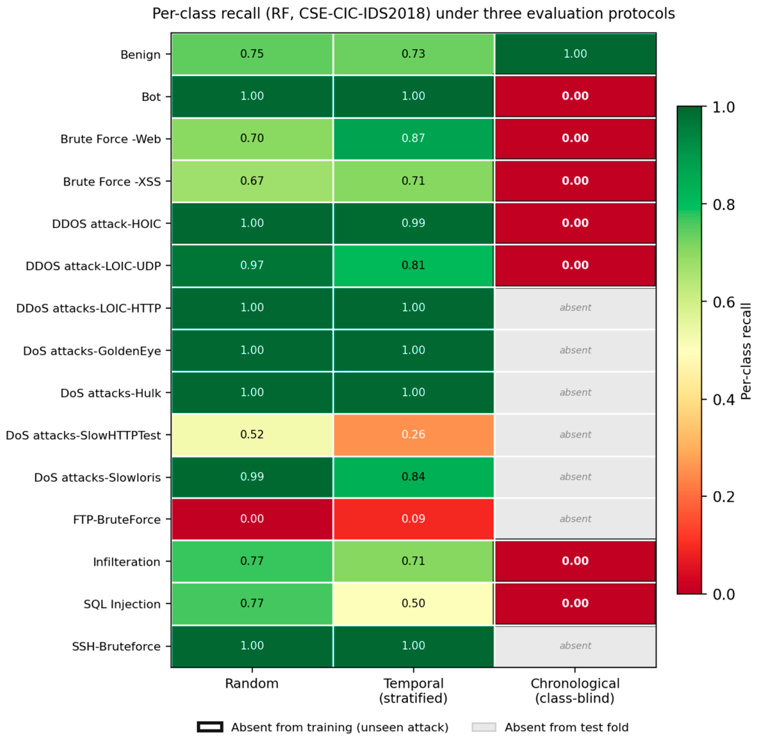
This interpretation is the central finding. The near-equality of random and stratified-temporal performance shows that time alone does not destroy performance: when every attack class is represented in training, a model evaluated on strictly later traffic of those same classes still performs well, so within-class distribution drift is mild over this horizon. The collapse under class-blind chronological splitting is therefore driven primarily by unseen-attack generalization failure, the time-ordered cut places whole attack families (e.g. HOIC, LOIC-UDP, SSH-Bruteforce) after the split, and the model scores zero on every class it never trained on. Consistent with this, the class-blind protocol exhibits a very low false-positive rate (RF: 0.0011) despite near-zero macro-F1: the failure mode is missed detections of unseen attacks, not false alarms.
Figure 3.
Per-class recall (RF, CSE-CIC-IDS2018) under the three protocols. Cells show recall; black borders mark classes absent from training under that protocol (structurally unseen attacks), and grey cells mark classes absent from the test fold (recall undefined). Under random and stratified-temporal splitting recall is uniformly high, because every attack family is represented in training. Under class-blind chronological splitting the day-structured capture confines whole families to one side of the time cut: seven attack families are unseen in training and score exactly zero recall, while only the persistently-present Benign class is detected, directly explaining the near-zero macro-F1 alongside the near-zero false-positive rate.
Figure 3.
Per-class recall (RF, CSE-CIC-IDS2018) under the three protocols. Cells show recall; black borders mark classes absent from training under that protocol (structurally unseen attacks), and grey cells mark classes absent from the test fold (recall undefined). Under random and stratified-temporal splitting recall is uniformly high, because every attack family is represented in training. Under class-blind chronological splitting the day-structured capture confines whole families to one side of the time cut: seven attack families are unseen in training and score exactly zero recall, while only the persistently-present Benign class is detected, directly explaining the near-zero macro-F1 alongside the near-zero false-positive rate.
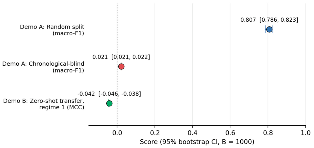
Significance and leakage controls. Bootstrapping the RF macro-F1 (B = 1000) gives random 0.807 (95% CI [0.786, 0.823]) versus class-blind 0.021 (95% CI [0.0213, 0.0216]); the intervals are far from overlapping. A paired bootstrap of the random vs. class-blind gap yields 0.782 (95% CI [0.746, 0.801]) with empirical p < 0.001 (no resample reversed the gap). The narrow interval for the class-blind protocol reflects degenerate near-constant predictions rather than high precision, and we note this in interpretation. A label-shuffle control, training on permuted labels under the random split, drops macro-F1 to 0.065, essentially the 1/15 ≈ 0.067 chance level, confirming the pipeline contains no harness leakage.
Figure 4.
Bootstrap 95% confidence intervals (B = 1000) for three headline quantities. The Demo A random and class-blind chronological macro-F1 intervals are far from overlapping, and the Demo B zero-shot MCC interval (regime 1, shown as a representative case) lies entirely below zero (dotted line), confirming that zero-shot transfer performs worse than chance; the regime-2 zero-shot MCC (−0.078, Table 4) is likewise negative. The intervals are tight enough that the whiskers are barely visible at this scale.
Figure 4.
Bootstrap 95% confidence intervals (B = 1000) for three headline quantities. The Demo A random and class-blind chronological macro-F1 intervals are far from overlapping, and the Demo B zero-shot MCC interval (regime 1, shown as a representative case) lies entirely below zero (dotted line), confirming that zero-shot transfer performs worse than chance; the regime-2 zero-shot MCC (−0.078, Table 4) is likewise negative. The intervals are tight enough that the whiskers are barely visible at this scale.
6.2. Cross-Dataset Transfer Collapses Zero-Shot; Recalibration Repairs Confidence but Restores Discrimination only Unevenly
Table 4 reports zero-shot transfer from CSE-CIC-IDS2018 to each CIC-DDoS2019 regime, followed by the calibration-buffer sweep. Zero-shot transfer collapses in both regimes: MCC −0.043 (regime 1) and −0.078 (regime 2), both below zero, i.e. worse than chance, with ECE ≈ 0.91–0.93 indicating confidently wrong predictions and macro-F1 near 0.03–0.05. The transferred model is badly miscalibrated and non-discriminating out of the box on both targets. Two cell-level patterns are worth noting so they are not mistaken for errors. First, at zero-shot the macro-F1 (e.g. 0.027) exceeds the weighted-F1 (0.002): the model predicts almost everything as benign, which earns a little F1 on the rare benign class but essentially zero on the dominant ddos class, and because ddos carries ~97% of the weight the weighted average is dragged to near zero while the unweighted macro average is not. Second, the zero-shot false-positive rate is very low (0.006–0.008) despite worse-than-chance MCC, for the same reason seen in Demo A: predicting benign almost everywhere produces few benign-flagged-as-attack errors, so the failure mode is missed attacks, not false alarms.
The calibration buffer repairs confidence in both regimes but has a strikingly different effect on discrimination. Confidence recovers consistently: ECE falls from 0.93 → 0.11 (regime 1) and 0.91 → 0.02 (regime 2) as the time-ordered buffer grows, with the Brier score tracking it down. Discrimination, however, recovers only partially and unevenly. In regime 1 it barely moves, MCC rises from −0.04 only to 0.26 at best, so recalibration leaves the model weakly discriminating at best. In regime 2 the same procedure substantially rescues the model: MCC climbs from −0.08 to 0.71 and macro-F1 to 0.85 with just a 1% buffer. The contrast is explained by the macro-AUPRC, which measures ranking quality independent of the decision threshold: in regime 1 it is poor throughout (≈ 0.54, barely above chance), so no amount of recalibration can help, the model never ranked the classes well. In regime 2 it is high even at zero-shot (≈ 0.87), meaning the model could separate the classes all along but applied the wrong decision threshold; here the buffer corrects the threshold and discrimination is recovered. The decisive observation is that the calibration metrics do not predict which case one is in: ECE recovers to a low value in both regimes, yet behind that apparent calibration success the discriminative outcome ranges from near-useless (regime 1) to largely restored (regime 2). An operator watching only ECE or Brier would see “recovery” in both and could not tell that one model remained almost worthless. Figure 5 shows this dissociation between uniform confidence recovery and regime-dependent discrimination recovery.
The practical implication is that repairing confidence does not guarantee a usable model. The buffer restored useful discrimination in one regime and barely helped in the other, and the calibration metrics that are easiest to monitor gave no warning of the difference. The mechanism we propose, that recalibration can fix a misplaced threshold (regime 2) but cannot repair genuinely poor ranking (regime 1), is consistent with the AUPRC pattern, though we do not separately ablate it. Whether a small target buffer suffices is therefore an empirical, per-deployment question, not something a practitioner can assume; safe practice is to track discrimination metrics (MCC, AUPRC) directly and to treat retraining, not recalibration, as the default response to drift.
6.3. A Distributional Explanation for the Transfer Collapse
Why does transfer collapse? Table 5 and Figure 6 report PSI and KS between the two datasets over the 45 common-core features. 36 of 45 features exceed the severe-drift threshold of PSI ≥ 0.25; of the remaining nine, two show moderate drift (0.10 ≤ PSI < 0.25) and only seven are essentially stable (PSI < 0.10). This count is not an artifact of PSI’s unboundedness: the bounded KS statistic gives a near-identical picture, with 37 of 45 features exceeding KS ≥ 0.10 and 33 of 45 exceeding KS ≥ 0.20, so the two metrics agree on the scale of the shift. The bounded KS statistic also confirms the magnitude without PSI’s inflation: the top-drifting features reach KS ≈ 0.76–0.79, meaning their empirical distributions barely overlap. The label distribution itself shifts severely: within the shared {benign, ddos} space, benign prevalence falls from ~38% in CSE-CIC-IDS2018 to ~3% in CIC-DDoS2019.
The drifting features are exactly those one would expect to separate the two regimes: forward packet-length and segment-size statistics, inter-arrival times, and packet rates. These are the hallmarks of high-rate DDoS flood traffic, which differs fundamentally from the mixed enterprise flows of CSE-CIC-IDS2018. The distributional analysis thus explains the collapse directly: the features a 2018-trained model relies on are precisely the ones that have moved, which is why zero-shot transfer performs worse than chance. This aggregate analysis accounts for the zero-shot collapse common to both regimes; it does not, on its own, explain why one regime proved recoverable under recalibration and the other did not. That asymmetry is governed by post-transfer ranking quality (the AUPRC contrast in Section 6.2) rather than by the marginal feature drift measured here, and separating the two would require per-regime drift attribution that we leave to future work.
7. Discussion
A single-split score is not evidence of deployment readiness. Our central finding is that, holding model and data fixed, switching the evaluation protocol moves macro-F1 from 0.81 to 0.02. Any IDS result reported on a single random split is therefore consistent with both a strong detector and one that collapses the moment the traffic mix changes; the random split cannot distinguish them. Reporting at least one time-aware split is the minimum needed to tell these cases apart. This conclusion echoes, in the NIDS setting, the temporal-bias critique of Pendlebury et al. [10] and the broader pitfalls catalogued by Arp et al. [11].
Unseen attacks, not gradual drift, drive the within-dataset collapse. Our stratified-temporal control isolates the mechanism: performance survives when class coverage is held fixed but collapses when time-ordering hides whole attack families. This distinction matters for practitioners, who should expect their largest failures at the introduction of new attack types rather than from slow distributional drift in known ones.
Repairing confidence does not guarantee a usable model. The cross-dataset experiment shows that calibration and discrimination recover differently under drift. A small time-ordered target buffer makes the model’s confidence trustworthy again in both regimes (ECE falling to ≤ 0.11 at the largest buffer), but its effect on the decisions themselves is regime-dependent: in one regime discrimination barely improves (MCC ≈ 0.26), while in the other it is substantially restored (MCC ≈ 0.71). Critically, both regimes end up looking well-calibrated (low ECE), so an operator monitoring only ECE or Brier could not tell a recovered model from one that is still largely non-discriminating. Discrimination metrics (MCC, AUPRC) should therefore be tracked alongside calibration metrics, and since a calibration buffer cannot be relied upon to restore discrimination, retraining rather than recalibration is the safer default response to feature drift.
Feature extraction is part of the data-generating process. The 24→45 feature-alignment step (Section 5.1) is a reminder that the table a model sees is produced by a specific extractor with specific naming conventions. Silent schema mismatch can halve the usable cross-dataset feature space before any modelling begins; we recommend that cross-dataset studies report their feature-alignment procedure explicitly.
Limitations. The study covers two flow-based CIC datasets and offline drift only; it does not address heterogeneous IoT telemetry, online streaming detection, or full retrain-versus-recalibrate adaptation. The cross-dataset label space is necessarily restricted to {benign, ddos}, the families the two datasets share. Two further caveats bound the cross-dataset claims specifically. First, both datasets originate from the same producer (CIC) and the same feature extractor (CICFlowMeter); this controls extractor-induced schema differences but also means our transfer result has not been tested against a genuinely independent collection pipeline, so the drift we measure may understate what occurs across labs and tools. Second, the two captures differ in task as well as distribution, CSE-CIC-IDS2018 is mixed multi-attack enterprise traffic while CIC-DDoS2019 is DDoS-only, so the zero-shot collapse reflects a combination of feature drift and a narrowing of the attack mix, and we do not claim to isolate drift from this task shift. Third, the recalibration result rests on two transfer regimes; the regime-dependent recovery we report should be read as a cautionary observation rather than a general law, and whether the inconsistency persists across many target distributions is an open question we leave to future work. The PSI/KS analysis (Section 6.3) establishes that the shared features move substantially but is associational: we show the features a 2018-trained model relies on are precisely those that shift, not a causal ablation retraining on drift-robust features. These boundaries are deliberate, they keep every claim measurable, and they define the future-work agenda in Section 8.
8. Recommendations and Future Work
8.1. Recommendations for IDS Evaluation
- Report at least one time-aware split (chronological or stratified-temporal) in addition to any random split, and report the gap.
- When claiming generalization, report at least one cross-dataset or cross-regime transfer result.
- Retain timestamps, day identifiers, and scenario identifiers as metadata even when they are excluded from model inputs.
- State the exact dataset release, cleaning script, label mapping, and feature-alignment procedure.
- Report calibration (ECE, Brier) and discrimination (MCC, AUPRC) metrics, plus false-positive burden, never accuracy or weighted-F1 alone, especially under class imbalance.
- Accompany headline gaps with confidence intervals and a leakage control.
8.2. Future Work
This study deliberately scopes to two flow-based datasets and offline analysis. Natural extensions include: heterogeneous IoT and IIoT telemetry datasets, where modality and schema drift add further dimensions; online streaming detectors (e.g. ADWIN, DDM, EDDM) for real-time drift alarms; additional drift measures such as KL divergence and multivariate tests; and a full retrain-versus-recalibrate adaptation study quantifying recovery cost. We are pursuing these directions in ongoing work.
9. Conclusion
We presented a controlled study of how evaluation choices shape reported performance for flow-based intrusion detection. Holding the model, features, and data fixed, the train-test protocol alone moves macro-F1 from ~0.81 to ~0.02, a model-agnostic gap that a stratified-temporal control attributes to unseen-attack coverage rather than gradual drift. Extending to cross-dataset transfer, we showed that a model trained on CSE-CIC-IDS2018 collapses to worse-than-chance on both CIC-DDoS2019 regimes, and that a small time-ordered calibration buffer reliably repairs confidence but restores discrimination only unevenly, substantially in one regime, barely in the other, with calibration metrics giving no indication of which. A distributional analysis ties the transfer collapse to pervasive feature drift in timing, packet-length, and rate statistics. Taken together, these results argue that single-split accuracy is not evidence of deployment readiness: a credible NIDS evaluation should report a time-aware split alongside any random split, include a cross-dataset or cross-regime transfer result, and track discrimination metrics rather than relying on calibration or weighted-F1 alone. The pipeline, statistics, and controls are fully specified (Appendix A) to support replication and extension to the broader settings outlined in Section 8.
Data Availability
Use of AI Tools
Generative AI tools were used to assist with manuscript preparation, including drafting, copy-editing, formatting, and figure-caption refinement. They were not used to generate, analyse, or interpret the experimental results, all of which were produced by the author’s own code and pipeline. The author reviewed and verified all content and takes full responsibility for the final text.
Conflicts of Interest
The author declares no conflicts of interest.
Appendix A. Reproducibility Manifest
This appendix specifies the exact inputs and settings needed to reproduce every reported number. The complete code, configuration, and synonym map are available from the author on request.
A.1 Dataset releases and files. CSE-CIC-IDS2018: official CIC “CSE-CIC-IDS2018 on AWS” release [1], the per-day *_TrafficForML_CICFlowMeter.csv exports. CIC-DDoS2019: official CIC release [3], the 01-12 capture (training-day, regime 1) and the 03-11 capture (testing-day, regime 2). Timestamps are parsed day-first; four stray repeated header rows in the 2018 CSVs are dropped.
A.2 Post-cleaning, post-cap class counts. CSE-CIC-IDS2018: 875,951 flows over fifteen native classes (Benign 160,939 down to FTP-BruteForce 54; Heartbleed absent after cleaning); the 200,000-per-class cap does not bind here, since the largest class is below it. CIC-DDoS2019 regime 1: ~2.10M flows; regime 2: ~1.17M flows (regime 2 includes the Portmap family, absent from regime 1); here the cap is active, bounding the large DDoS families. Each class is capped at 200,000 flows by uniform-across-time sampling, applied after chronological ordering so that temporal structure is preserved.
A.3 Label harmonisation. Native labels map to families: benign→benign; FTP/SSH brute force→brute_force; Bot→botnet; DoS Hulk/GoldenEye/Slowloris/SlowHTTPTest→dos; DDoS LOIC-HTTP/HOIC/LOIC-UDP→ddos; web XSS/SQL/brute force→web; Infiltration→infiltration. All CIC-DDoS2019 reflection/amplification families (including Portmap) map to ddos. The shared cross-dataset family space is {benign, ddos}.
A.4 Feature harmonisation. A naïve column intersection of the two CICFlowMeter exports yields 24 shared features; canonicalising naming differences (e.g. bwd_pkt_len_max↔bwd_packet_length_max, flow_byts/s↔flow_bytes/s, ack_flag_cnt↔ack_flag_count, seg_size_avg↔seg_size_mean) recovers 45 semantically aligned features, used for all cross-dataset analysis: fwd/bwd packet-length min/max/mean/std, fwd/bwd segment-size mean, flow/fwd/bwd IAT min/max/mean/std, idle and active min/max/mean/std, flow duration, flow/fwd/bwd packets-per-second, flow bytes-per-second, fwd/bwd header length, subflow fwd/bwd packets, down/up ratio, fwd act-data packets, fwd PSH flags, and CWE flag count.
A.5 Models. Random Forest (300 trees, unbounded depth, class_weight="balanced_subsample"); LightGBM (400 estimators, learning rate 0.05, 63 leaves, class_weight="balanced"); two-layer MLP (StandardScaler → hidden layers 128 and 64, ReLU, Adam, α = 10⁻⁴, max 300 iterations). All use random seed 0; all other hyperparameters are library defaults, and no per-protocol or per-dataset tuning was performed.
A.6 Statistic settings. PSI: 10 equal-frequency bins on the reference distribution, with ε = 10⁻⁶ added to empty bins before the logarithm; bands < 0.10 negligible, 0.10–0.25 moderate, ≥ 0.25 severe (heuristic). KS: two-sample, computed on raw feature values. ECE: top-label ECE with 15 equal-width confidence bins. Brier: multiclass (one-vs-all) form, range [0, 2] for two classes. Bootstrap: B = 1000 resamples, 2.5/97.5 percentiles, test set subsampled to 100,000 flows. AUPRC: macro-average of per-class one-vs-rest average-precision scores.
References
- Canadian Institute for Cybersecurity, “CSE-CIC-IDS2018 on AWS,” University of New Brunswick. [Online]. Available: https://www.unb.ca/cic/datasets/ids-2018.html.
- I. Sharafaldin, A. H. Lashkari, and A. A. Ghorbani, “Toward generating a new intrusion detection dataset and intrusion traffic characterization,” in Proc. 4th Int. Conf. Information Systems Security and Privacy (ICISSP), 2018, pp. 108–116.
- Canadian Institute for Cybersecurity, “DDoS Evaluation Dataset (CIC-DDoS2019),” University of New Brunswick. [Online]. Available: https://www.unb.ca/cic/datasets/ddos-2019.html.
- M. Cantone, C. Marrocco, and A. Bria, “Machine learning in network intrusion detection: A cross-dataset generalization study,” IEEE Access, vol. 12, pp. 144489–144508, 2024. [CrossRef]
- L. Liu, G. Engelen, T. Lynar, D. Essam, and W. Joosen, “Error prevalence in NIDS datasets: A case study on CIC-IDS-2017 and CSE-CIC-IDS-2018,” in Proc. IEEE Conf. Communications and Network Security (CNS), 2022, pp. 254–262. [CrossRef]
- A. Raskovalov, N. Gabdullin, and V. Dolmatov, “Investigation and rectification of NIDS datasets and standardized feature set derivation for network attack detection with graph neural networks,” arXiv:2212.13994, 2022.
- C. Guo, G. Pleiss, Y. Sun, and K. Q. Weinberger, “On calibration of modern neural networks,” in Proc. 34th Int. Conf. Machine Learning (ICML), 2017, pp. 1321–1330.
- J. C. Platt, “Probabilistic outputs for support vector machines and comparisons to regularized likelihood methods,” in Advances in Large Margin Classifiers, A. J. Smola et al., Eds. Cambridge, MA: MIT Press, 1999, pp. 61–74.
- J. Gama, P. Medas, G. Castillo, and P. Rodrigues, “Learning with drift detection,” in Advances in Artificial Intelligence - SBIA 2004, Lecture Notes in Computer Science, vol. 3171, 2004, pp. 286–295.
- F. Pendlebury, F. Pierazzi, R. Jordaney, J. Kinder, and L. Cavallaro, “TESSERACT: Eliminating experimental bias in malware classification across space and time,” in Proc. 28th USENIX Security Symposium, 2019, pp. 729–746.
- D. Arp, E. Quiring, F. Pendlebury, A. Warnecke, F. Pierazzi, C. Wressnegger, L. Cavallaro, and K. Rieck, “Dos and don’ts of machine learning in computer security,” in Proc. 31st USENIX Security Symposium, 2022, pp. 3971–3988.
- J. G. Moreno-Torres, T. Raeder, R. Alaiz-Rodriguez, N. V. Chawla, and F. Herrera, “A unifying view on dataset shift in classification,” Pattern Recognition, vol. 45, no. 1, pp. 521–530, 2012. [CrossRef]
- M. Sarhan, S. Layeghy, N. Moustafa, and M. Portmann, “NetFlow datasets for machine learning-based network intrusion detection systems,” in Big Data Technologies and Applications (BDTA), Lecture Notes of ICST, 2020, pp. 117–135. [CrossRef]
- M. P. Naeini, G. F. Cooper, and M. Hauskrecht, “Obtaining well calibrated probabilities using Bayesian binning,” in Proc. AAAI Conf. Artificial Intelligence, vol. 29, no. 1, 2015, pp. 2901–2907.
- A. H. Lashkari, G. Draper-Gil, M. S. I. Mamun, and A. A. Ghorbani, “Characterization of Tor traffic using time based features,” in Proc. 3rd Int. Conf. Information Systems Security and Privacy (ICISSP), 2017, pp. 253–262.
- N. Siddiqi, Credit Risk Scorecards: Developing and Implementing Intelligent Credit Scoring. Hoboken, NJ, USA: Wiley, 2006.
- NIST/SEMATECH, “Kolmogorov-Smirnov goodness-of-fit test,” in e-Handbook of Statistical Methods. [Online]. Available: https://www.itl.nist.gov/div898/handbook/eda/section3/eda35g.htm.
Figure 1.
Macro-F1 under the three evaluation protocols, by model. Random and stratified-temporal agree; the class-blind chronological protocol collapses to near zero across all three model families.
Figure 1.
Macro-F1 under the three evaluation protocols, by model. Random and stratified-temporal agree; the class-blind chronological protocol collapses to near zero across all three model families.
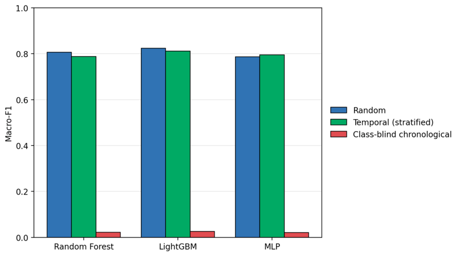
Figure 2.
Expected Calibration Error under the three protocols. Under class-blind chronological splitting the models are not merely less accurate, their confidence becomes meaningless (ECE ≈ 0.73–0.83).
Figure 2.
Expected Calibration Error under the three protocols. Under class-blind chronological splitting the models are not merely less accurate, their confidence becomes meaningless (ECE ≈ 0.73–0.83).
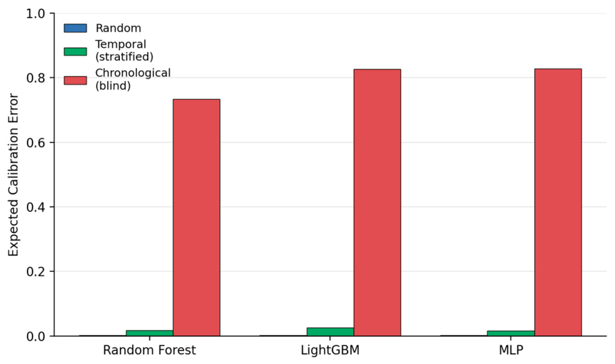
Figure 5.
Cross-dataset transfer across two regimes with a time-ordered calibration buffer (calibration on the earliest fraction of each capture, evaluation on later traffic). ECE (red) recovers in both regimes as the buffer grows, but discrimination (MCC, blue) recovers very unevenly: weakly in regime 1 (to ≈ 0.26) and strongly in regime 2 (to ≈ 0.71). Calibration improves strongly in both regimes, but the discrimination outcomes differ sharply, so calibration metrics alone do not indicate whether recalibration has restored a usable model.
Figure 5.
Cross-dataset transfer across two regimes with a time-ordered calibration buffer (calibration on the earliest fraction of each capture, evaluation on later traffic). ECE (red) recovers in both regimes as the buffer grows, but discrimination (MCC, blue) recovers very unevenly: weakly in regime 1 (to ≈ 0.26) and strongly in regime 2 (to ≈ 0.71). Calibration improves strongly in both regimes, but the discrimination outcomes differ sharply, so calibration metrics alone do not indicate whether recalibration has restored a usable model.
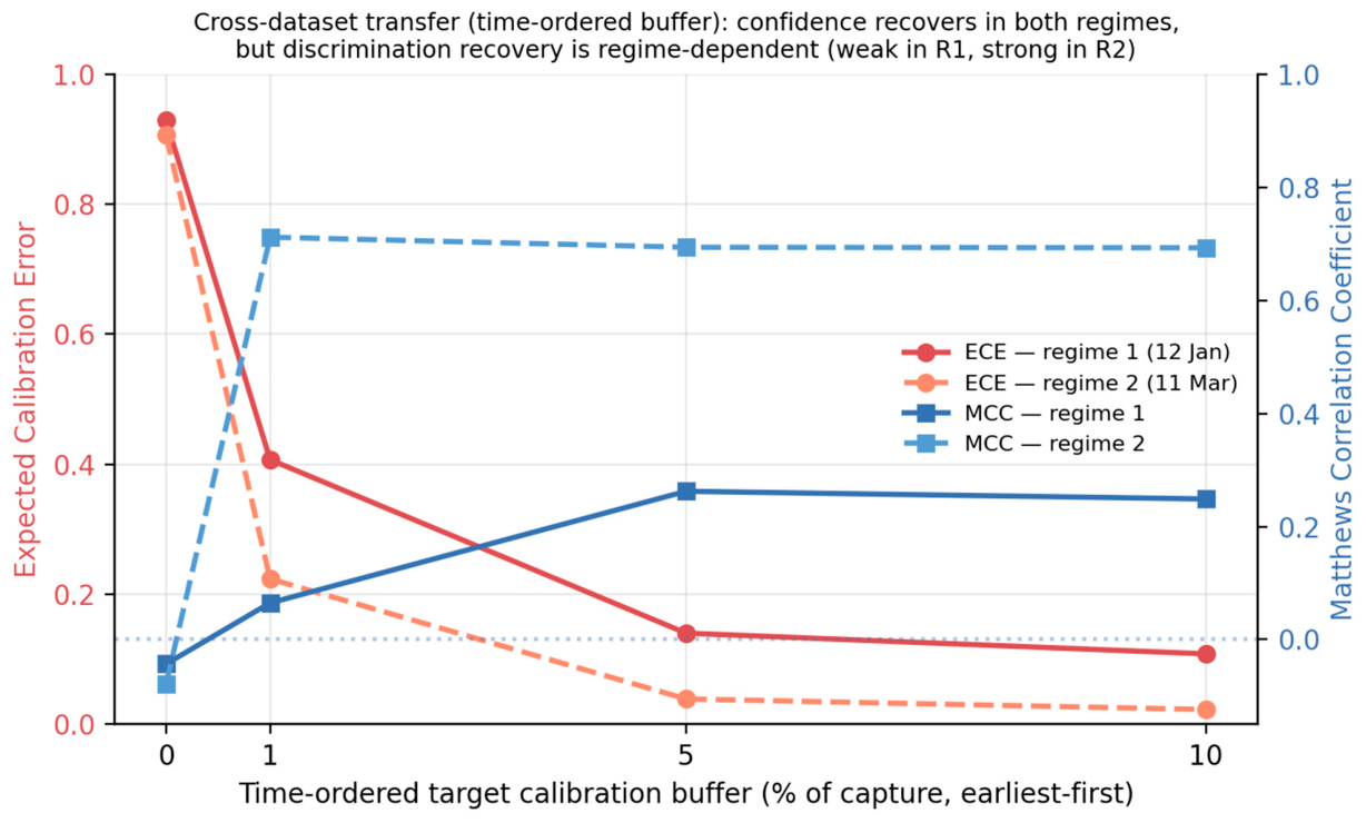
Figure 6.
Cross-dataset feature drift ranked by KS statistic. The most-drifted features are forward packet-length, inter-arrival-time, and packet-rate statistics, the signature of high-rate DDoS floods versus mixed enterprise traffic, directly explaining the zero-shot transfer collapse in Section 6.2.
Figure 6.
Cross-dataset feature drift ranked by KS statistic. The most-drifted features are forward packet-length, inter-arrival-time, and packet-rate statistics, the signature of high-rate DDoS floods versus mixed enterprise traffic, directly explaining the zero-shot transfer collapse in Section 6.2.
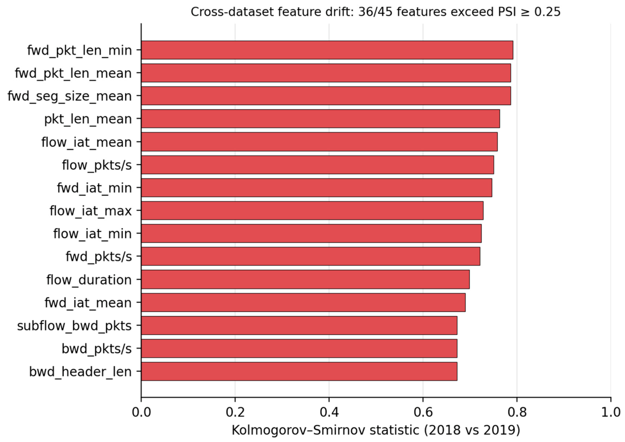

Table 1.
The two flow-based datasets used in this study.
| Dataset | Collection context | Attack coverage | Drift relevance |
|---|---|---|---|
| CSE-CIC-IDS2018 | Enterprise/cloud AWS testbed; traffic organized by scenario days | Brute force, botnet, DoS, DDoS, web attacks, infiltration | Enterprise baseline; strong temporal-leakage risk if day/scenario structure is ignored |
| CIC-DDoS2019 | DDoS-focused CIC testbed; two separate capture days | Reflection/amplification DDoS families; Portmap appears only in the testing-day regime | Attack-scope and label-distribution drift; severe class imbalance; novel-family transfer target |
Table 2.
Drift layers exercised in this study.
| Drift layer | Meaning | Where it appears here |
|---|---|---|
| Feature drift | The distribution of measured variables changes | 36/45 common-core features shift between datasets (Section 6.3) |
| Label-distribution drift | The frequency of benign vs. attack classes changes | Within the shared {benign, ddos} space, benign prevalence falls from ~38% (CSE-CIC-IDS2018) to ~3% (CIC-DDoS2019) |
| Predictive concept drift | The feature→label relationship changes | Zero-shot cross-dataset transfer collapses to MCC ≤ 0 (Section 6.2) |
| Temporal/context drift | The order or context of traffic affects evaluation | Random vs. chronological splitting changes macro-F1 by 0.78 (Section 6.1) |
Table 3.
Demo A: within-CSE-CIC-IDS2018 performance under three evaluation protocols.
| Model | Protocol | Macro-F1 | Weighted-F1 | MCC | ECE |
|---|---|---|---|---|---|
| RF | Random | 0.807 | 0.921 | 0.907 | 0.002 |
| RF | Temporal (stratified) | 0.787 | 0.907 | 0.891 | 0.018 |
| RF | Chronological (class-blind) | 0.021 | 0.051 | 0.026 | 0.734 |
| LightGBM | Random | 0.824 | 0.921 | 0.909 | 0.003 |
| LightGBM | Temporal (stratified) | 0.811 | 0.900 | 0.884 | 0.026 |
| LightGBM | Chronological (class-blind) | 0.025 | 0.057 | 0.057 | 0.826 |
| MLP | Random | 0.786 | 0.901 | 0.885 | 0.002 |
| MLP | Temporal (stratified) | 0.796 | 0.898 | 0.880 | 0.016 |
| MLP | Chronological (class-blind) | 0.021 | 0.050 | 0.010 | 0.829 |
Table 4.
Demo B: cross-dataset transfer (RF, 45 common-core features, {benign, ddos}). Brier is the multiclass form, bounded in [0, 2] for two classes.
Table 4.
Demo B: cross-dataset transfer (RF, 45 common-core features, {benign, ddos}). Brier is the multiclass form, bounded in [0, 2] for two classes.
| Regime | Setting | Macro-F1 | Weighted-F1 | MCC | AUPRC | FP-rate | Brier | ECE |
| 1 (12 Jan) | Zero-shot | 0.027 | 0.002 | −0.043 | 0.551 | 0.006 | 1.776 | 0.928 |
| 1 | Buffer 1% | 0.207 | 0.356 | 0.065 | 0.540 | 0.037 | 0.650 | 0.407 |
| 1 | Buffer 5% | 0.547 | 0.893 | 0.262 | 0.540 | 0.147 | 0.151 | 0.140 |
| 1 | Buffer 10% | 0.542 | 0.888 | 0.249 | 0.539 | 0.186 | 0.130 | 0.108 |
| 2 (11 Mar) | Zero-shot | 0.046 | 0.005 | −0.078 | 0.874 | 0.008 | 1.729 | 0.906 |
| 2 | Buffer 1% | 0.853 | 0.973 | 0.712 | 0.870 | 0.177 | 0.157 | 0.224 |
| 2 | Buffer 5% | 0.847 | 0.972 | 0.694 | 0.870 | 0.268 | 0.043 | 0.039 |
| 2 | Buffer 10% | 0.846 | 0.971 | 0.693 | 0.870 | 0.268 | 0.042 | 0.023 |
Table 5.
Top-ranked drifting features between CSE-CIC-IDS2018 and CIC-DDoS2019 (by KS). Rows are ordered by KS, the bounded magnitude we rely on; PSI is shown for completeness and is not monotonic with KS because it inflates without bound when distributions barely overlap (Section 5.2).
Table 5.
Top-ranked drifting features between CSE-CIC-IDS2018 and CIC-DDoS2019 (by KS). Rows are ordered by KS, the bounded magnitude we rely on; PSI is shown for completeness and is not monotonic with KS because it inflates without bound when distributions barely overlap (Section 5.2).
| Feature | PSI | KS |
|---|---|---|
| fwd_pkt_len_min | 2.51 | 0.792 |
| fwd_pkt_len_mean | 2.63 | 0.787 |
| fwd_seg_size_mean | 2.63 | 0.787 |
| pkt_len_mean | 4.23 | 0.763 |
| flow_iat_mean | 3.89 | 0.758 |
| flow_pkts/s | 3.53 | 0.750 |
| fwd_iat_min | 6.35 | 0.747 |
Disclaimer/Publisher’s Note: The statements, opinions and data contained in all publications are solely those of the individual author(s) and contributor(s) and not of MDPI and/or the editor(s). MDPI and/or the editor(s) disclaim responsibility for any injury to people or property resulting from any ideas, methods, instructions or products referred to in the content. |
© 2026 by the authors. Licensee MDPI, Basel, Switzerland. This article is an open access article distributed under the terms and conditions of the Creative Commons Attribution (CC BY) license (http://creativecommons.org/licenses/by/4.0/).
Copyright: This open access article is published under a Creative Commons CC BY 4.0 license, which permit the free download, distribution, and reuse, provided that the author and preprint are cited in any reuse.


