

Submitted:
10 June 2026
Posted:
11 June 2026
You are already at the latest version
Abstract
This study developed an integrated GIS-based Multi-Criteria Decision Analysis (GIS-MCDA) framework based on hydrological marginality, soil suitability, land cover marginality, slope, social marginality, and contaminated land indicators to identify and classify marginal and underutilized lands in Leon County, Florida using the Analytic Hierarchy Process (AHP) and weighted overlay analysis. The AHP results assigned the highest weights to hydrological conditions (36%) and soil suitability (24%), indicating their dominant influence on land marginality. The final marginality model classified the study area as low marginality/highly suitable (24.19 %), slightly marginal (39.17 %), moderately marginal (2.48 %), high marginality (30.66 %), and very high marginality and underutilization potential (3.5 %). According to sensitivity analysis, hydrology, soil, and social emphasis models showed results that were relatively stable compared to the AHP-weighted baseline model. However, an equal-weight model yielded a lower estimate. A 2-mile marginality increment was used to develop a future scenario. The results showed an estimated increase of about 23,762 acres of highly marginal land. These findings show that combining environmental and socioeconomic indicators can improve the identification of marginal and underutilized land and support sustainable land-use planning, restoration targeting, and future agricultural or bioenergy suitability assessments.
Keywords:
underutilized land
; marginal land
; land suitability
; GIS-MCDA
; spatial analysis
; analytical hierarchy process (AHP)
; socioeconomic vulnerability
; weighted overlay analysis
; random forest (RF)
1. Introduction
Marginal land is land with low productivity that provides little economic return due to various biophysical, social, and economic constraints [1]. Underutilized land refers to idle or abandoned land, which is currently not being used to its full productive potential [2]. Underutilized and marginal land is subject to economic constraints as its production is not cost-effective and profitable under current management techniques and policies. From biophysical perspective, underutilized and marginal land is also subject to natural constraints like steep slopes, weather conditions, and soil quality. In addition, social perspective including human factors such as workforce and distance from infrastructure also plays a crucial role.
The demand for food is increasing at unprecedented rates, while the agricultural land base is shrinking in many regions. This dynamics of population growth [3], land fragmentation [4], and urbanization and infrastructure have led to significant land-use change [5]. Global food production must increase by 50-60% by 2050 to meet the demand of the growing population [6]. Steering agricultural expansion toward marginal and underutilized lands is highly suggested to avoid the environmental consequences of clearing high-value ecosystems [1].
Globally, marginal land is estimated to cover approximately 2.7 billion hectares, of which 1.5 billion hectares is currently unused but suitable for agricultural cultivation [7]. On the global scale, marginal land is increasingly viewed as essential for a bio-based economy, with projections to supply 14-85% of the total global biomass demand by 2050 [8]. In the United States, estimates of marginal agricultural land are substantial but vary depending on the evaluation criteria, ranging from 10 million to 173 million hectares [2]. In a study focused on 10 Midwest U.S. states, approximately 11 million hectares of non-forested marginal land has been identified, which is suitable for bioenergy production [9]. Florida has 17.16 million acres of forested land, representing 50% of the state’s total acreage [10]. In regions like the Florida Panhandle, the focus on underutilized or sensitive land often involves monitoring forest health to protect these resources from invasive species [10]
Marginal land plays a vital role in bioenergy production and is viewed as a win for growing dedicated energy crops like switchgrass, miscanthus, and short-rotation woody crops, as they avoid direct competition with food crops on prime land [2,9]. Marginal land also provides ecosystem services by repurposing and facilitating carbon sequestration, groundwater recharge, and wildlife habitat restoration [11].
Leon County, Florida, was selected as the study area due to its diverse range of landscapes, including urban, peri-urban, forested, agricultural, and wetland areas. In Leon County, Florida, the number of farms increased 14%, from 325 to 375, between 2017 and 2022, respectively, but total farmland area decreased from 91,730 acres to 70,058 acres in the same period according to the USDA Census of Agriculture. Land fragmentation of Leon County positions it as a critical region for case study, as urban expansion exerts pressure on rural property values, declining the scale of local economies and accelerating farmland conversion [12]. In addition, the county faces several environmental constraints, including wetlands, hydrological limitations, fragmented land cover, and contaminated land. These factors limit conventional agricultural activities, creating opportunities for alternative land use, such as ecological restoration, carbon sequestration, and biomass production [13]. There is a need for localized research combining environmental and socio-economic factors to identify marginalized and underutilized lands at the county level, which justifies the use of Leon County as the testbed for the case study. The result will help assess how GIS-based multiple-criteria methods facilitate sustainable land-use planning.
GIS and MCDA techniques are useful tools for integrating diverse datasets into an analytical framework. Among these methods, the Weighted Linear Combination (WLC) is commonly used to evaluate land suitability by combining multiple criteria into a single composite index. It allows decision makers to aggregate multiple, often conflicting criteria, such as physical and socioeconomic criteria, into a single suitability score for each location [14]. GIS is a tool for data acquisition, storage, manipulation, and visualization in the form of suitability maps [5]. MCDA provides a structured set of techniques for weighting and ranking alternatives based on conflicting criteria, thereby effectively incorporating stakeholder values into the spatial model [5,14]. WLC is the most widely used MCDA technique for land suitability assessments [15,16]. This technique allows decision-makers to evaluate land suitability by combining multiple spatial factors based on their relative importance [16]. The process typically follows a three-step workflow to integrate diverse datasets: standardization, weighting, and aggregation.
The goal of this study is to identify and classify marginal and underutilized land in Leon County, Florida by integrating environmental and socioeconomic data within a GIS-based MCDA framework. The specific objectives are to apply AHP to 1) determine the relative importance of environmental and socioeconomic criteria influencing marginal and underutilized land distribution, 2) validate model performance using sensitivity analysis, correlation analysis, and random forest regression, and 3) simulate future changes in marginality under projected urban expansion conditions. The results aim to support policy decisions and land use planning by highlighting areas where underutilized land overlaps with socially vulnerable communities.
2. Literature Review and Conceptual Contexts
2.1. The Concept of Marginal Underutilized Land
The concept of marginal and underutilized land, usually associated with economic theories, has evolved since the 19th century, which is defined through specific economic and social lenses and is often described as “idle,” “waste,” “abandoned,” or “degraded” land [3]. Specifically, marginal land refers to the dynamic land that depends on the specific purposes, time, and place of use. The term is defined based on economic and biophysical perspectives. Notably, David Ricardo’s Theory of Rent firstly introduced the definition of marginal [6]. According to this theory, marginal land is primarily defined as land where cost-effective production is not profitable under the current market conditions, cultivation techniques, and agricultural policies. This definition is not far from the modern one, in which, in modern modeling, it is often identified as land with potential profit equal to or less than zero [2].
From the biophysical perspective, land characterized by natural constraints such as high acidity, salinity, steep slopes, extreme aridity, or shallow soil depth is considered marginal land [1]. According to FAO and UNEP, a land can also be classified as marginal if it supports only 40% or less of its total productivity potential [6]. Marginality is not necessarily a permanent state as a land can be highly suitable for uses other than food crops, such as grazing, forestry, or dedicated bioenergy crops like Arundo donax [1,2].
Underutilized land refers to areas that are physically available but functionally neglected or sub-optimally employed [4]. The land has low human employment levels relative to its potential, often due to excessive exploitation followed by abandonment [14]. Underutilized land is often covered with groves, shrubs, weeds, grass, or open fields. For instance, in Indonesia, a large part of the land that remains unused for 3 to 5 years is turned over to growing grasses and shrubs, which is categorized as underutilized land [4]. Socio-economic factors contribute to land underutilization, including land fragmentation, distance from modern infrastructure, rural depopulation, and aging workforces [1]. Although the terms of “marginal” and “underutilized” are sometimes used interchangeably, there is a major difference between them. Natural factors often constrain marginal land, whereas underutilized land might be suitable for agriculture but remains idle due to external factors.
2.2. Land-Use Change and Agricultural Land Decline
The global agricultural industry is going through great transformations induced by a combination of demographic, economic, and environmental pressures, with a demand projected to double by 2050 [3]. Land use change refers to the modification in utilization or management of a particular area of land, such as converting a forest into a farm or a rural field into an urban center [17]. Key concepts of land-use change include human-driven processes, particularly population growth, that drive demand of land for agriculture, housing, and energy [18]. Agricultural land decline occurs when the total land dedicated to farming decreases. While many areas of the world experience agricultural expansion at the expense of deforestation, other areas face decline due to urbanization, policy shifts, or environmental factors [17].
Primary drivers of land use changes are: (1) population growth and urbanization – In Indonesia, paddy fields are converted to non-agricultural uses at a rate of 90,000 to 110,000 hectares per year, with 75% of the fields shifted to housing [19]. (2) economic marginality – Land is usually abandoned when cost-effective production is no longer possible under the current market conditions. These conditions can be caused by fluctuating commodity prices, rising production costs, or inflation [2]. (3) land fragmentation – Agricultural productivity is threatened by fragmented ownership, often due to inheritance patterns, in countries such as China and Slovakia. Smallholder ownership makes efficient production difficult, which leads to an increase in abandoned lands [4]. (4) environmental degradation – In the lower Mississippi Alluvial Valley, intensive row cropping and chemical fertilizer use have reduced the soil’s ability to grow crops, leading to marginality [2].
Contaminated land, such as brownfields and former industrial sites, represents a specific category of constrained land, which is unsuitable for primary uses such as food production without significant remediation. [11]. Identifying contaminated land requires an assessment of biophysical and anthropogenic factors that limit land productivity and usability [3]. Failure to account for contaminated land can lead to overestimating available land resources, resulting in inappropriate land-use recommendations.
2.3. Integration of Biophysical and Socioeconomic Factors
The combination of biophysical and socioeconomic factors as resource standards is recommended for robust land-use suitability analysis, which transitions from a purely technical, data-driven approach to a collaborative, multifaceted planning framework [14]. This approach combines objective biophysical factors with subjective human values and economic realities to yield accurate, acceptable results. GIS-MCDA and machine learning approaches are two ways of integration. GIS-MCDA provides tools for storing and manipulating spatial data. At the same time, MCDA, for example, the WLC method, multiplies normalized weights by standardized factor values to create a composite stability score.[1].
Machine learning such as Random Forests or MaxEnt is a modern approach to use algorithms to integrate complex datasets. A typical study on land suitability modeling was by Wotlolan (2021), which integrated geospatial data and artificial intelligence by building a data cube of 100 geospatial layers, including climate, water, and accessibility to predict land suitability for agro-silvopastoral systems with high accuracy. The Integration of biophysical and socioeconomic factors gives a clearer understanding of the land compared to the use of separate data alone. In addition, it helps to account for constraints like political, social, and environmental factors [3].
2.4. Research Gap
Despite advances in GIS-based land suitability analysis, several gaps remain. Firstly, many studies prioritize biophysical factors with limited attention to socioeconomic conditions. Secondly, environmental constraints, such as land contamination, are often excluded from analyses, leading to incomplete assessments of land suitability. Thirdly, there is a lack of localized studies that integrate multiple data sources to identify marginal and underutilized land at the county or regional level. This study addresses these gaps by developing an integrated framework that combines biophysical, socioeconomic, and environmental data to identify marginal and underutilized land in Leon County, Florida. By applying a WLC approach within a GIS environment, this study provides a comprehensive assessment of land suitability and its relationship with socioeconomic vulnerability.
3. Materials and Methods
3.1. Study Area
The study covers Leon County, Florida, which is located in the United States’ Florida Panhandle (latitude 30.44 °N, longitude 84.28 °W) (Figure 1). The county encompasses a mix of urban, peri-urban, and rural landscapes, with Tallahassee as the state’s capital and primary urban center. According to the U.S. Census Bureau, the county covers 702 sq mi, of which 667 sq mi is land, and the rest is water. As of the 2020 Census, the total population is 292,198. About 19% of the residents were under 18, and 14.7% were 65 or older. From an environmental and climatic standpoint, the county is shaped by extensive riparian wetlands, seasonal floodplains, karst topography, and a longleaf pine ecosystem, with mean annual precipitation exceeding 1,400 mm.
Leon County was selected as the study area due to:
- The county faces significant urban growth pressure – According to USDA data (2017-2021), the number of farms increased from 325 to 375 (approximately 14%). However, total farmland acreage declined from 91,730 acres to 70,058 acres (approximately 24%).
- The county features multiple land cover features (Figure 2). Multiple environmental constraints reduce conventional agriculture use but create opportunities for sustainable land use, such as ecological restoration, carbon sequestration, and biomass production. Table 1 shows the land cover classification codes used in the study.
- No prior study has combined environmental constraints with socioeconomic constraints to map marginal and underutilized land, making Leon County an ideal candidate for developing a transferable analytical framework.
3.2. Data Sources
The analysis integrated both biophysical and socioeconomic datasets to capture multiple dimensions of land suitability. The data sets used in this study are summarized in Table 2, as follows:
All datasets were harmonized with respect to projection, spatial extent, and resolution prior to analysis. ESRI ArcGIS Pro Version 3.6.0 was used for data processing, raster standardization, terrain analysis, and multi-criteria modeling, including Project Raster, Extract by Mask, Reclassify, Raster Calculator, and Slope. These tools collectively allow for the development of a Weighted Marginality surface through spatial overlay analysis. A 30-meter cell size, Common Snap raster for the NLCD dataset, and NAD 1983 State Plane Florida North FIPS 0930 feet were used to ensure projection consistency.
3.3. Marginality Criteria Development
Land marginality was developed and operationalized as a spatial layer based on six criteria. Higher values in each layer indicate stronger environmental and socioeconomic constraints, indicating higher marginality and reduced land productivity and usability.
3.4. Reclassification and Standardization
Variables, including soil suitability, slope, hydrological conditions, land cover, contamination, and socioeconomic factors, were standardized to a common marginality scale ranging from 1 (lowest marginality) to 10 (highest marginality) to enable the integration within a multi-criteria framework using ArcGIS Pro’s reclassify tool. A cell with a score of 10 in any layer indicates the most constrained condition for that criterion, while a score of 1 indicates the least constrained. Table 3 describes the reclassification scheme for marginality standardization.
3.5. Analytical Hierarchy Process (AHP) Weighting
Analytic Hierarchy Process (AHP), a structured mathematical technique for multi-criteria decision making (MCDM) to derive relative weights of importance for various criteria through human judgment was used in this study [15,20]. AHP was developed by Thomas L. Saaty in the 1970s, and is widely utilized in GIS to assess land suitability by integrating objective spatial data with subjective value judgments [21,22]
A pairwise comparison matrix was constructed for the six marginality criteria using a nine-point scale, where 1 indicates equal importance, and 9 indicates extreme importance of one criterion over another. The detailed pairwise comparison is shown in Table 4, and Table 5 shows the AHP pairwise-derived criterion weights following matrix normalization. Each cell in the matrix represents the relative importance of the row criterion compared to the column criterion. The matrix was then normalized by dividing each cell by its column sum, and criterion weights were derived as the row averages of the normalized matrix [23].
3.5.1. Consistency Analysis of the AHP Matrix
The responses were organized into a pairwise comparison matrix [24]. The weights were derived by calculating the principal eigenvector corresponding to the largest eigenvalue (λmax) of the matrix using (Eq 1), and then normalized so the weight summed to 1 [20]:
where is the weighted sum vector, is the weight vector, and is the number of criteria. The consistency of the pairwise judgment was evaluated using the consistency ratio (CR) (Eq. 2), which provides a measure of the degree of logic and consistency in the expert judgment [25]. CR was calculated by comparing the inconsistency of the matrix to a random index. If CR is less than 0.1 (10%), the judgments are considered consistent, and the weights are reliable [26].
where and RI is the Random Consistency Index for a matrix of size n (RI = 1.24 for n = 6). The Consistency Ratio (CR) was below the acceptable threshold of 0.10, CR≈0.037, indicating logical consistency in the weighting structure and that the pairwise judgments were not random.
3.6. Weighted Linear Combination (WLC) Model
In spatial analysis, derived weights were applied to map layers using the WLC method [1]. Each pixel’s value in a criterion map was multiplied by its AHP weight, and the results were summed to produce a final suitability index map [24,27]. The Weighted Linear Combination algorithm (Eq. 3), within the class of local operators, was used to obtain the suitable marginal degree for each cell in the study area.
where M is the final weighted marginality score, Wi is the weight assigned to criterion I, Xi is the standardized marginality score for criterion I, and n is the number of criteria.
Weights were assigned based on the relative importance of each factor in determining land marginality. The weighting system was established based on the impact each criterion had on the degree of land marginality, as determined from past GIS-MCDA analyses of suitability studies. The factors related to hydrology and soils were assigned higher weights due to their significant impacts on limiting agriculture and protecting the environment. The applied model was shown in Equation 4:
MLI was computed cell-by-cell across the full county extent using the ArcGIS Pro Raster Calculator. The resulting continuous surface ranges from approximately 2.4 to 8.9, representing a gradient from minimally constrained land (low MLI) to maximally constrained or underutilized land (high MLI). The composite raster was then classified into five marginality categories using equal-interval classification, ranging from Class 1 (very low marginality) to Class 5 (high marginality / high underutilization potential). Urban areas (medium- and high-intensity developed land) and open water bodies were masked from the final output using ArcGIS Pro’s Extract by Mask tool, ensuring that the model focuses exclusively on realistically available land surfaces.
3.7. Sensitivity Analysis
Sensitivity analysis (SA), a critical stage in evaluating MCDA models, was used to check the reliability and robustness of the results by assessing how uncertainties in input parameters affected the final output [28]. Four alternative scenarios (Table 6) were developed and compared against the baseline AHP-derived scenario in terms of 1) the total acreage classified as high marginality (Classes 4 and 5), 2) the spatial overlap of high-marginality areas between scenarios, and 3) shifts in the spatial distribution of marginality hotspots across the county.
3.8. Correlation Analysis
Using ArcGIS Pro’s Create Random Points tool, 1000 random points were distributed across the study area to assess the relationships among individual layers and the final composite MLI (Figure 3). The correlation matrix was used to1) quantify the relative strength of each individual criterion’s relationship with the final MLI, 2) identify patterns of co-variation among criteria (e.g., correlation between hydrological and land cover layers, given the spatial overlap of wetlands in both datasets), and 3) detect potential multicollinearity that could inflate the influence of correlated variables in the composite model. Correlation results informed the subsequent machine learning validation and supported the interpretation of the dominant drivers of land marginality in Leon County.
3.9. Machine Learning Validation
GIS-based machine learning validation, a multi-step process that combines traditional statistical metrics with advanced spatial strategies, is essential to ensure model reliability [29,30]. Especially, Random Forest, a commonly used machine learning algorithm, was used in this study by constructing multiple decision trees from bootstrap samples of the training data and aggregate their predictions [29]. The predictor variables included five standardized raster variables (Hydro, Soil, Slope, Social, and Contam.) from 1000 random sample points, which served as the modeling dataset. The land cover marginality layer was intentionally excluded from the Random Forest model due to its high correlation with the hydrological marginality layer (r > 0.80), which would introduce multicollinearity and lead to inflated or unstable variable importance estimates. This exclusion followed standard practice in machine learning feature selection for spatially correlated predictors. The target variable for the RF model was the final AHP-derived MLI value at each sample point.
3.10. Future Scenario Modeling
A scenario based on 2035 was developed to project future land expansion and land use. The main goal is to provide spatial insight into areas most likely to experience development pressure and to promote sustainable land-use planning and conservation targets. A buffer zone was generated by adding a 2-mile marginality increment, applied uniformly across the buffer to maintain methodological simplicity and transparency, while acknowledging that actual development intensity varied with proximity to roads, infrastructure, and zoning designations. All pixels were represented to reflect land use expansion. This buffer extent is consistent with documented rates of urban fringe expansion observed in the county between 2000 and 2022. The methodological workflow is shown in Figure 4.
3.7. Area Estimation
The area of each class was calculated using raster attribute tables. Cell counts were converted to area using the raster’s spatial resolution, and results were expressed in acres using equation 5 and as percentages of the total study area using equation 6, which enabled quantitative comparison of land categories:
4. Results
4.1. Individual Marginality Factors
Hydrological marginality is shown in Figure 5(a), where darker areas indicate a marginality score of 10, and 9 indicates higher hydrological constraints, which include wetlands, saturated soils, flood-prone areas, and areas with water-related limitations. A lighter color indicates drier, more stable conditions and is considered lower-marginality. The hydrological constraints are widespread across the county, especially along drainage networks and wetlands. Excessive moisture and flooding reduce land suitability and lead to land marginality.
Figure. 5(b) presents the land cover marginality. Higher marginality patterns are concentrated in urbanized and environmentally restricted landscapes, which are related to developed lands, dense forest cover, water bodies, and wetlands, while lower marginality levels are observed in agriculturally usable lands. Figure. 5(c) shows the spatial distribution of contaminated and non-contaminated land within Leon County. The red shows the contaminated area, while the gray shows the non-contaminated area. The contaminated areas are concentrated primarily within the central portion of the county near the urbanized area. Figure 5(d) illustrates the spatial distribution of the soil. Areas with poor soil and drainage limitations are distributed in the southern part of the county and exhibit higher marginality. Lower marginality values are associated with more suitable agricultural soils.
Figure 5(e) shows the spatial distribution of social marginality across Leon County. Lighter yellow tones represent lower social marginality concentrated in eastern and central Leon County. These areas highly correspond to favorable socioeconomic conditions. Dark red and orange tones distribute across the central, northern, and southern parts of the study area, indicating greater social marginality and indicating multiple socioeconomic limitations. Figure. 5(f) presents the spatial distribution of slope-derived marginality across the county based on the DEM-based terrain analysis. Orange and red tones in steeper terrain correspond to higher marginality, and yellow tones represent lower values in flatter areas. Steeper areas are considered more marginal because steeper slopes increase erosion risk, reduce mechanized farming efficiency, and limit land use.
4.2. Final Marginality Classification
The GIS-based weighted overlay analysis successfully identified the spatial pattern of marginal and underutilized land in Leon County, Florida. The outputs reveal spatial variation in marginality conditions across the county, influenced by both biophysical and socioeconomic constraints. The candidate land is classified into five distinct categories according to levels of marginality and potential underutilization. The categories are divided into Class 1, representing low marginality and high suitability, and Class 5, denoting very high marginality and high underutilization potential. Based on the results, high marginality is more commonly associated with hydrologic constraints, poor soil quality, fragmented land cover, and lower socioeconomic suitability.
The weighted marginality surface shown in Figure 6 represents the integrated effect of multiple biophysical and socioeconomic variables, including soil suitability, hydrological condition, slope, land cover, contamination areas, and socioeconomic indicators. The resulting raster shows a range of values from 2.4 to 8.9. Higher marginality values are observed in the south and southwest portions of the county, indicating an overlap of multiple constraints. On the other side, lower marginality values are shown in the north regions of the county, suggesting relatively favorable conditions for existing land use.
The map in Figure 6 shows discernible spatial distributions of the various land classifications in Leon County. Table 7 below shows the area and percentage distribution of the marginality derived for the AHP baseline-weighted overlay model in Leon County, Florida.
The combined (high marginality) class 4 and (very high marginality and underutilization potential) class 5 categories represent approximately 152,771.24 acres, accounting for 34.16% of the total study area. In terms of their spatial location, they were scattered throughout the southern and eastern portions of the study area. Poor soil conditions, hydrological constraints, fragmented land cover, and low socioeconomic suitability often characterize these territories. The results of this final classification indicate that factors such as hydrologic limitations, land cover types, soil capabilities, and socioeconomics strongly influence land marginality in Leon County.
4.3. Sensitivity Analysis Result
To evaluate the stability of the weighted overlay model, a sensitivity analysis was conducted by emphasizing variables and developing alternative weighting scenarios. Figure 7 shows a map of different scenarios and alternative weighting conditions in Leon County, Florida. The hydrology, soil, and social emphasis scenarios produce results that remain relatively close to the baseline model. A combination of class 4 and class 5 areas was compared for each scenario. Based on the analysis, the hydrology emphasis scenario resulted in 142,258 acres, the soil emphasis resulted in 151,887 acres, and the social emphasis resulted in 149,130 acres of class 4 and class 5 recorded areas. In contrast, 33,909 acres of class 4 and 5 areas were calculated under the equal-weight scenario.
4.4. Correlation Analysis Result
Pearson correlation analysis reflects the relationship between each variable and the AHP-based final marginality model (Table 8). Hydrological marginality shows the strongest positive relation with the final model (r=0.743), followed by soil marginality (r=0.704) and land cover marginality (r=0.628). In contrast, social marginality and contaminated land show a weaker positive relationship with the AHP-based final marginality model (r=0.242 and r=0.019, respectively). In addition, slope marginality shows a weak negative correlation with the final model (r = -0.332), reflecting low relief across the study area.
4.5. Machine Learning Validation Result
The Random Forest analysis identified hydrological marginality as an influential predictor of final marginality, accounting for 65.8% of total variable importance. Soil and social marginality rank second and third among the strongest predictors, with influential coefficients of 26.5% and 5.8%, respectively. On the contrary, slope and contamination are comparatively minor, with combined levels below 2%. The validation results from Random Forest were consistent with the AHP Weighting structure and correlation analysis. The result confirms that hydrological and soil constraints play a dominant role in identifying marginal and underutilized land within the county.
4.6. Future Scenario Result
An urban expansion scenario for the future was developed to assess potential shifts in marginal land distribution under anticipated development pressures in 2035. Table 9 illustrates scenarios that account for the impact of urban influence on existing developed lands and for a higher marginality rating in proposed urban expansion areas.
Based on the results of the future scenario, there was a marked increase in moderately high, highly marginal, and highly marginal lands in Leon County. The total of Class 4 and Class 5 land increased from about 152,771 acres (34.14%) to about 176,534 acres (36.59%) under the future urban expansion scenario in 2035, which indicates an estimated increase of about 23,762 acres of highly marginal lands. Geographically, the increase in marginality occurred mostly in peri-urban areas near Tallahassee and along corridors of existing development (Figure 8). The urban expansion scenario shows that continued urban development could lead to increased land fragmentation and environmental/land-use restrictions in parts of the county.
5. Discussion
This study uses environmental and socioeconomic indicators to identify marginal and underutilized lands in Leon County, Florida, by developing a GIS-MCDA framework. The results show that hydrological and social indicators are major drivers of marginality patterns across the study area. Areas characterized by wetlands, saturated soil, poor drainage, and flood-prone conditions show higher marginality, especially in the south and southwestern part of the study area. The study area was classified into 5 Classes: lower marginality/highly suitable (class-1), slightly marginal(class-2), moderately marginal (class-3), high marginality and very high marginality(class-4), and underutilization potential (class-5) by the AHP weighted overlay baseline model. Approximately 34.14% of the study area falls under classes 4 and 5. The most influential spatial constraint in the study area was hydrological marginality.
In the sensitivity analysis, 4 models were developed. Three models emphasized hydrology, soil, and social weights, resulting in relatively stable outcomes under alternative conditions to the AHP-weighted overlay baseline model. An equal-weight model for all indicators was also developed, resulting in a lower high marginality estimate, indicating that environmental and social scenarios cannot realistically be represented by equal weight. A machine learning validation using Random Forest analysis further strengthens the dominance of hydrological and soil constraints in identifying hydrological marginality as a strong predictor, with approximately 92.2% of the combined total variable importance. The projection of marginal lands in 2035 was also developed and showed an increase in marginal land, suggesting that continued urban expansion may intensify fragmentation and environmental constraints in the study area.
5.1. Policy Implications and Sustainability
The GIS-based methodology framework has integrated multiple environmental and socioeconomic datasets to identify highly marginal and underutilized land. Higher marginality is associated with areas coinciding with wetlands, poorly drained soils, fragmented land cover, and lower socioeconomic activity. These areas are not suitable for conventional land use, but other forms of sustainable utilization may still be viable. This suggests opportunities for alternative and suitable land management strategies in Leon County, Florida. The study highlights that marginal land need not be interpreted as unusable.
This farmwork can support land-use planning, conservation prioritization, remediation efforts, and sustainable resource management at the local and regional levels. In relation to the future urban growth scenario, it is notable how much the peri-urban development pressures are beginning to affect land marginality. As seen in the predicted increase of around 23,762 acres of Class 4 and Class 5 lands, continued outward growth of urban areas near Tallahassee will lead to greater land fragmentation and decreased land-use flexibility over time. Growing development pressures can also lead to increased land sensitivity and underdevelopment. Based on sensitivity analysis, the developed GIS-MCDA model shows considerable resistance to realistic changes in the weighting scheme. Due to the stability within different weight variations, it is safe to conclude that the spatial distribution of marginal lands will not be affected in any noticeable way due to slight adjustments in the weighting scheme.
5.2. Strengths and Limitations of the Study
One of the strengths of this study was the combination of environmental and socioeconomic dimensions using the AHO weighted overlay analysis, sensitivity analysis, correlation analysis, and Random Forest validation analysis. A future scenario modeling approach further strengthened the final marginality assessment in the study area. In addition, the study examines both environmental and socioeconomic dimensions, unlike previous studies that primarily focus on biophysical constraints.
There are several limitations to be acknowledged as well.
- The AHP weighting approach is dependent on expert judgment, which may introduce subjectivity into the weighting structure. Although the consistency ratio indicated acceptable logical consistency, a sensitivity analysis was conducted
- Future urban expansion was developed using a simplified buffer-based approach. Nevertheless, a more detailed future prediction model can be developed using Automata or CA-Markov simulation.
- Landcover marginality was excluded from the Random Forest validation due to multicollinearity. This might reduce the machine learning evaluation of land cover influence in the framework, even though this improved the model interpretability.
6. Conclusions
The study shows the importance of integrating environmental and socio-economic factors to identify marginal and underutilized land and inform future land-use planning and sustainable strategies. Areas that fall into categories of low marginality/highly suitable, slightly marginal, and moderately marginal present opportunities for sustainable land use such as biomass production, sustainable agricultural production, or conservation. In contrast, areas under high marginality and very high marginality have underutilization potential that requires protection from intensified land-use pressure. This study can be a valuable source of information for policymakers, land-use planners, and resource managers to balance economic and infrastructure development, agricultural preservation, future urban growth management, and environmental sustainability, thereby supporting informed decision-making. The projected increase in highly marginal land under the 2035 urban expansion scenario shows the need for proactive planning strategies that minimize land fragmentation and protect environmentally sensitive landscapes. Future studies should include climate-related environmental variables, and a detailed predictive model can be developed using Automata or CA-Markov simulation to strengthen the applicability of the framework for regional sustainability planning and land management decision-making.
Author Contributions
Conceptualization, T.A.S. and H.H; methodology, T.A.S. and H.H.; software, T.A.S. and H.H.; validation, T.A.S. and H.H; formal analysis, T.A.S.; investigation, T.A.S. and H.H.; resources, V.I.; data curation, T.A.S. and H.H; writing and editing T.A.S., H.H, S.A.N., G.C., and V.B.; supervising and resource, H.H. All authors have read and agreed to the published version of the manuscript. .
Funding
This research received no external funding.
Institutional Review Board Statement
Not applicable.
Informed Consent Statement
Not applicable.
Data Availability Statement
The original data presented in the study are openly available. The county and census boundaries were obtained from the U.S. Census TIGER/Line database (https://www.census.gov. Accessed:29/04/2026), land cover data were obtained from the National Land Cover Database (NLCD) (https://www.usgs.gov Accessed:29/04/2026), soil data were obtained from Soil Survey Geographic Database (SSURGO) (https://www.nrcs.usda.gov/. Accessed:29/04/2026), elevation data were obtained from USGS 3D Elevation Program (3DEP) (https://www.usgs.gov/. Accessed:29/04/2026), socioeconomic data were obtained from American Community Survey (ACS) (https://www.census.gov/. Accessed:29/04/2026), and contaminated and brownfield data were obtained from Florida Department of Environmental Protection (FDEP), https://floridadep.gov/. Accessed:29/04/2026). The datasets used, processed, and analyzed, and the supporting data for this study will be made available by the authors on request.
Acknowledgments
The authors would also like to thank all colleagues for their support throughout the research period.
Conflicts of Interest
The authors declare no conflict of interest.
References
- Cervelli, E.; Recchi, P. F.; Fagnano, M.; Di Perta, E. Scotto; Pindozzi, S. Marginal lands between recovery and valorization. An inclusive definition to support bio-energy supply chains. The Southern Italy contexts case study. Agric. Syst. 2024, vol. 217, 103951. [Google Scholar] [CrossRef]
- Tiwari, P.; Poudel, K. P.; Yang, J.; Silva, B.; Yang, Y.; McConnell, M. Marginal agricultural land identification in the Lower Mississippi Alluvial Valley based on remote sensing and machine learning model. Int. J. Appl. Earth Obs. Geoinf. 2023, vol. 125, 103568. [Google Scholar] [CrossRef]
- Gibbs, H. K.; Salmon, J. M. Mapping the world’s degraded lands. Appl. Geogr. 2015, vol. 57, 12–21. [Google Scholar] [CrossRef]
- Mulyani, A.; Mulyanto, B.; Barus, B.; Panuju, D. R.; Husnain. Geospatial Analysis of Abandoned Lands Based on Agroecosystems: The Distribution and Land Suitability for Agricultural Land Development in Indonesia. Land 2022, vol. 11(no. 11), 2071. [Google Scholar] [CrossRef]
- Luan, C.; Liu, R.; Peng, S. Land-use suitability assessment for urban development using a GIS-based soft computing approach: A case study of Ili Valley, China. Ecol. Indic. 2021, vol. 123, 107333. [Google Scholar] [CrossRef]
- Jumaniyazov; Juliev, M.; Reimov, M.; Orazbaev, A.; Reymov, T.; Bekanov, K. Marginal lands: a review of papers from the Scopus database published in English for the period of 1979–2022. Soil Sci. Annu. 2023, vol. 74(no. 2), 1–13. [Google Scholar] [CrossRef]
- Csikós, N.; Tóth, G. Concepts of agricultural marginal lands and their utilisation: A review. Agric. Syst. 2023, vol. 204, 103560. [Google Scholar] [CrossRef]
- Pancaldi, F.; Trindade, L. M. Marginal Lands to Grow Novel Bio-Based Crops: A Plant Breeding Perspective. Front. Plant Sci. 2020, vol. 11, 227. [Google Scholar] [CrossRef]
- Gelfand; Sahajpal, R.; Zhang, X.; Izaurralde, R. C.; Gross, K. L.; Robertson, G. P. Sustainable bioenergy production from marginal lands in the US Midwest. Nature 2013, vol. 493(no. 7433), 514–517. [Google Scholar] [CrossRef]
- Robinson-Baker, A. M. S.; Haseeb, M.; Kanga, L. H. B. Diversity and Seasonal Abundance of the Pine Bark and Ambrosia Beetles in the Florida Panhandle. Insects 2025, vol. 16(no. 12), 1275. [Google Scholar] [CrossRef] [PubMed]
- Mellor, P.; Lord, R. A.; João, E.; Thomas, R.; Hursthouse, A. Identifying non-agricultural marginal lands as a route to sustainable bioenergy provision - A review and holistic definition. Renew. Sustain. Energy Rev. 2021, vol. 135, 110220. [Google Scholar] [CrossRef]
- Solís, D.; Alvarez, S.; Nguyen, L. Agriculture Under Pressure: The Economic, Environmental, and Development Drivers Transforming Florida Agriculture. Agriculture 2026, vol. 16(no. 6), 661. [Google Scholar] [CrossRef]
- The future of food and agriculture – Alternative pathways to 2050
- Malczewski, J. “GIS-based land-use suitability analysis: a critical overviewq”. [CrossRef]
- Ahmad Zaki, Z.; Yusup, M.; Che Abdullah, I.; Abdullah, Y. A.; Shah, A. S. Abdul Halim. LAND SUITABILITY ANALYSIS FOR URBAN GARDENING USING GIS-BASED MULTI-CRITERIA DECISION-MAKING APPROACH. Plan. Malays. 2023, vol. 21. [Google Scholar] [CrossRef]
- Karimi, H.; Amiri, S.; Huang, J.; Karimi, A. Integrating GIS and multi-criteria decision analysis for landfill site selection, case study: Javanrood County in Iran. Int. J. Environ. Sci. Technol. 2019, vol. 16(no. 11), 7305–7318. [Google Scholar] [CrossRef]
- Abdeta, D.; Begna, R.; Zerfu, H.; Alemayehu, A.; Ayana, A. N.; Tsegaye, N. T. Analyzing the extent and drivers of land use/land cover change in Southwestern Ethiopia. Discov. Sustain. 2024, vol. 5(no. 1), 505. [Google Scholar] [CrossRef]
- Msofe, N.; Sheng, L.; Lyimo, J. Land Use Change Trends and Their Driving Forces in the Kilombero Valley Floodplain, Southeastern Tanzania. Sustainability 2019, vol. 11(no. 2), 505. [Google Scholar] [CrossRef]
- El Baroudy, A. A. Mapping and evaluating land suitability using a GIS-based model. CATENA 2016, vol. 140, 96–104. [Google Scholar] [CrossRef]
- Tavana, M.; Soltanifar, M.; Santos-Arteaga, F. J. Analytical hierarchy process: revolution and evolution. Ann. Oper. Res. 2023, vol. 326(no. 2), 879–907. [Google Scholar] [CrossRef]
- Desta, M. D.; Tesseme, T.; Yigezu, T. T.; Nigussie, A. B. Assessment of landfill site suitability using GIS, remote sensing, and the multi-criteria decision-making (AHP) approach, Ethiopia. Geol. Ecol. Landsc. 2025, vol. 9(no. 2), 662–675. [Google Scholar] [CrossRef]
- Kayitete; Bakolo, C.; Tomlinson, J.; Fawcett, J.; Tuyisenge, M. F.; De Dieu Tuyizere, J. Applying Multi-Criteria Analysis in GIS to predict suitability for recreational green space interventions in Kigali City, Rwanda. Appl. Geomat. 2025, vol. 17(no. 1), 163–175. [Google Scholar] [CrossRef]
- Ligmann-Zielinska, A.; Jankowski, P. “A Framework for Sensitivity Analysis in Spatial Multiple Criteria Evaluation,” in Geographic Information Science. In Lecture Notes in Computer Science, vol. 5266.; Cova, T. J., Miller, H. J., Beard, K., Frank, A. U., Goodchild, M. F., Eds.; Springer Berlin Heidelberg: Berlin, Heidelberg, 2008; vol. 5266, pp. 217–233. [Google Scholar] [CrossRef]
- Hammami, S.; et al. Application of the GIS based multi-criteria decision analysis and analytical hierarchy process (AHP) in the flood susceptibility mapping (Tunisia). Arab. J. Geosci. 2019, vol. 12(no. 21), 653. [Google Scholar] [CrossRef]
- Tuğaç, G.; Tercan, A.; Torunlar, H.; Karakurt, E.; Usul, M. Agricultural land suitability assessment with GIS-based multi-criteria decision analysis and geostatistical approach in semi-arid regions. Soil Stud. 2023, vol. 12(no. 1), 15–29. [Google Scholar] [CrossRef]
- Chen, Y.; Yu, J.; Khan, S. Spatial sensitivity analysis of multi-criteria weights in GIS-based land suitability evaluation. Environ. Model. Softw. 2010, vol. 25(no. 12), 1582–1591. [Google Scholar] [CrossRef]
- AbdelRahman, A. E.; Saleh, A. M.; Arafat, S. M. Assessment of land suitability using a soil-indicator-based approach in a geomatics environment. Sci. Rep. 2022, vol. 12(no. 1), 18113. [Google Scholar] [CrossRef] [PubMed]
- Yu; Shahbaz, K.; Xevi, E. “A GIS-based sensitivity analysis of multi-criteria weights”.
- Meyer, H.; Reudenbach, C.; Wöllauer, S.; Nauss, T. Importance of spatial predictor variable selection in machine learning applications -- Moving from data reproduction to spatial prediction. Ecol. Model. 2019, vol. 411, 108815. [Google Scholar] [CrossRef]
- Ploton, P.; et al. , Spatial validation reveals poor predictive performance of large-scale ecological mapping models. Nat. Commun. 2020, vol. 11(no. 1), 4540. [Google Scholar] [CrossRef]
Figure 1.
Study area: Leon County, Florida, USA.
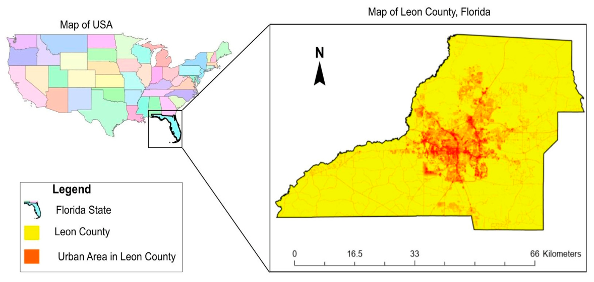
Figure 2.
Multiple land cover features classification in Leon County.
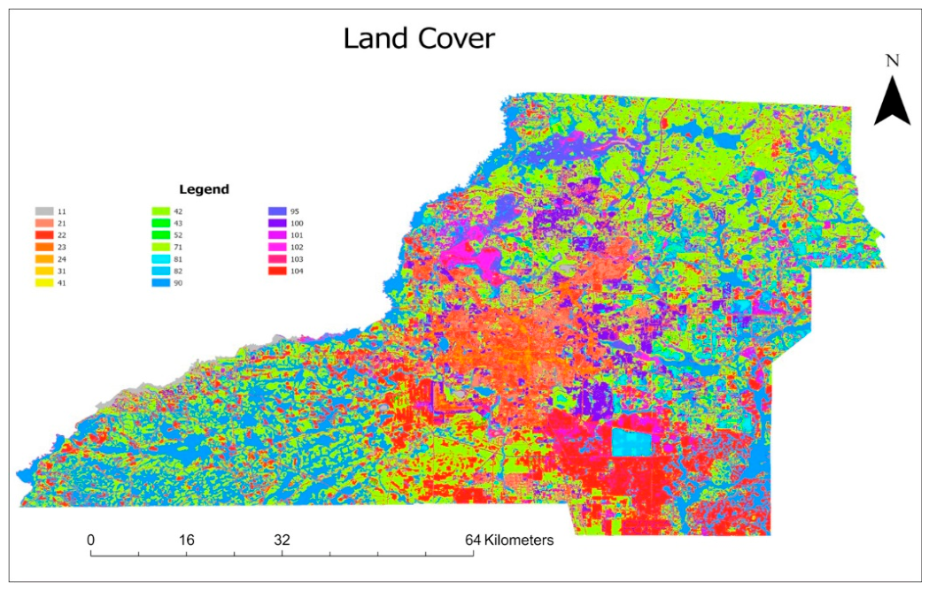
Figure 3.
Distribution of 1000 random points across the study area.
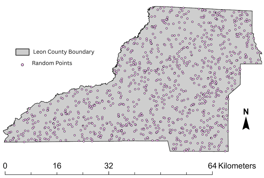
Figure 4.
Full methodological workflow diagram.
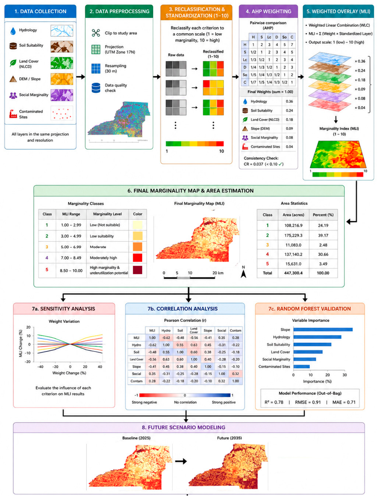
Figure 5.
Input layers used in the GIS-based marginal land suitability assessment for Leon County, Florida, including (a) hydrological marginality, (b) land cover marginality, (c) contaminated land constraints, (d) soil marginality, (e) social marginality, and (f) slope marginality.
Figure 5.
Input layers used in the GIS-based marginal land suitability assessment for Leon County, Florida, including (a) hydrological marginality, (b) land cover marginality, (c) contaminated land constraints, (d) soil marginality, (e) social marginality, and (f) slope marginality.
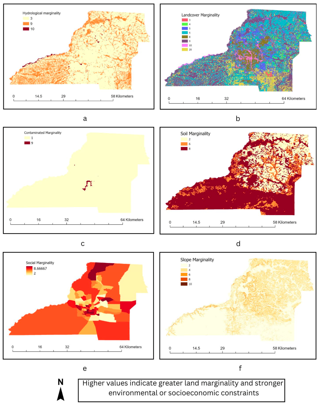
Figure 6.
Spatial distribution of marginal and underutilized land suitability classes in Leon County, Florida.
Figure 6.
Spatial distribution of marginal and underutilized land suitability classes in Leon County, Florida.
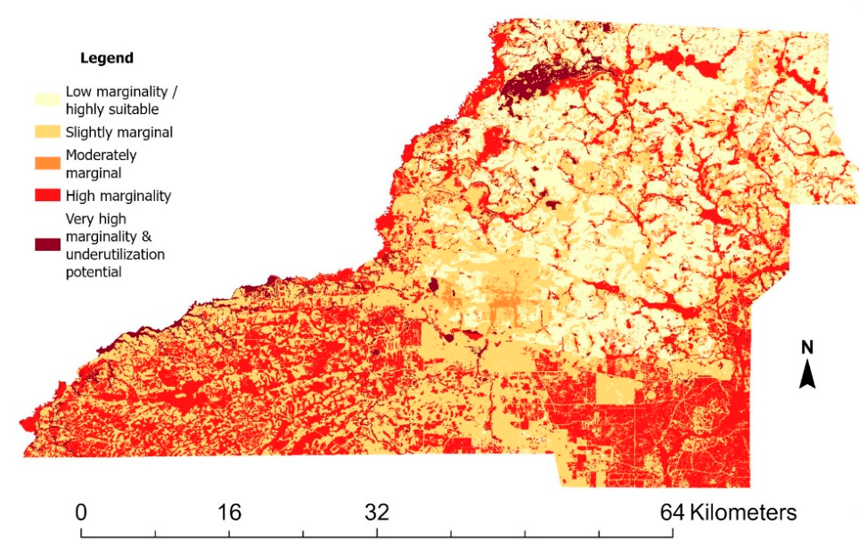
Figure 7.
Sensitivity analysis results under different weighting scenarios, including the AHP baseline, equal weights, soil emphasis, social emphasis, and hydrology emphasis.
Figure 7.
Sensitivity analysis results under different weighting scenarios, including the AHP baseline, equal weights, soil emphasis, social emphasis, and hydrology emphasis.
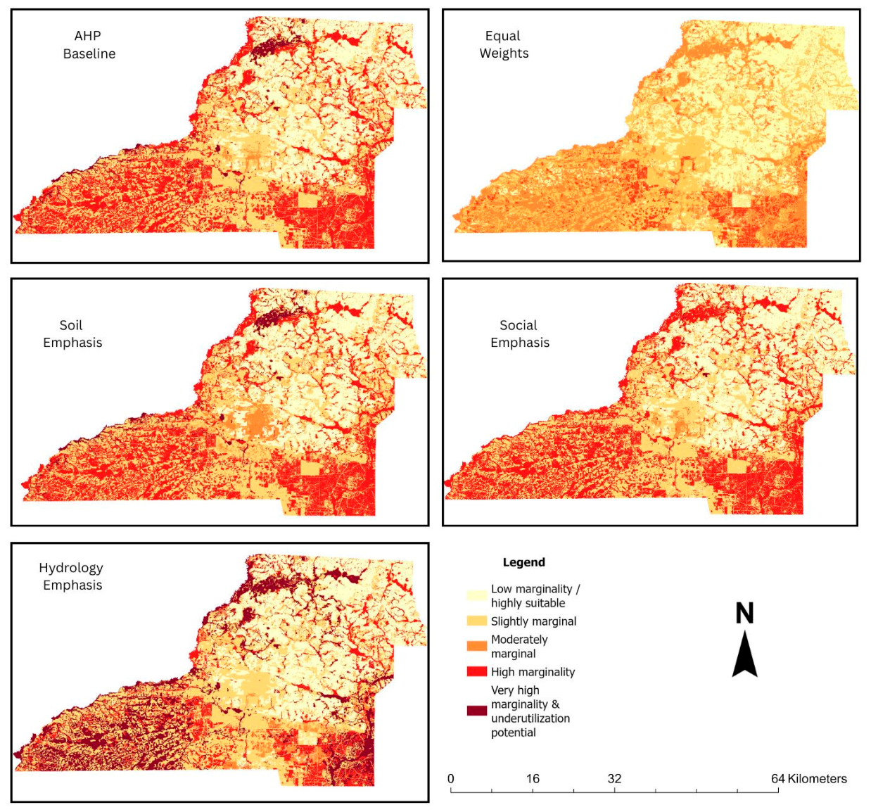
Figure 8.
Future 2035 marginality scenario under projected urban expansion conditions in Leon County, Florida.
Figure 8.
Future 2035 marginality scenario under projected urban expansion conditions in Leon County, Florida.
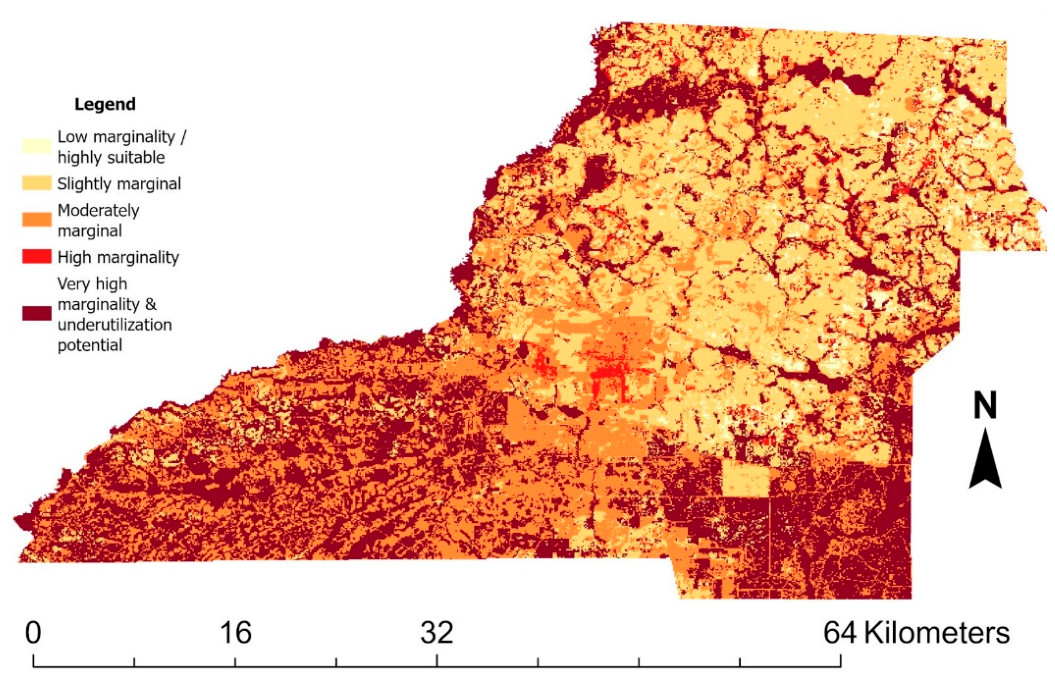

Table 1.
NLCD land cover classification codes used in the study.
| Code | Land Cover Class | Code | Land Cover Class |
|---|---|---|---|
| 11 | Open Water | 71 | Grassland/Herbaceous |
| 21 | Developed, Open Space | 81 | Pasture/Hay |
| 22 | Developed, Low Intensity | 82 | Cultivated Crops |
| 23 | Developed, Medium Intensity | 90 | Woody Wetlands |
| 24 | Developed, High Intensity | 95 | Emergent Herbaceous Wetlands |
| 31 | Barren Land | 100 | Moss |
| 41 | Deciduous Forest | 101 | Lichens |
| 42 | Evergreen Forest | 102 | Palustrine Forested Wetland |
| 43 | Mixed Forest | 103 | Palustrine Scrub/Shrub Wetland |
| 52 | Shrub/Scrub | 104 | Estuarine Forested Wetland |
Table 2.
Spatial datasets, data sources, spatial resolution, and analytical purpose used in the multi-criteria marginal land suitability analysis.
Table 2.
Spatial datasets, data sources, spatial resolution, and analytical purpose used in the multi-criteria marginal land suitability analysis.
| Datasets | Sources | Resolution | Uses |
|---|---|---|---|
| County & Census Boundaries | U.S. Census TIGER/Line database https://www.census.gov (Accessed: 29/04/2026) |
Vector | Define the study area |
| Land Cover Data | The National Land Cover Database (NLCD) 2021 is a 30 m resolution Landsat-based dataset. https://www.usgs.gov (Accessed: 29/04/2026) |
30 m | Identifying land-use classes, wetlands, water bodies, and developed areas. |
| Soil Data | Soil Survey Geographic Database (SSURGO) https://www.nrcs.usda.gov/ (Accessed: 29/04/2026) |
Vector / 30m | Providing detailed soil classification and farmland suitability information. |
| Elevation Data | USGS 3D Elevation Program (3DEP) at 1/3 arc-second resolution. https://www.usgs.gov/ (Accessed: 29/04/2026) |
1/3 arc-sec (~10 m) | Derive slope as a topographic constraint. |
| Socioeconomic Data | American Community Survey (ACS) https://www.census.gov/ (Accessed: 29/04/2026) |
Census tract | Provide information on population, income, and unemployment indicators. |
| Contaminated and brownfield site | Florida Department of Environmental Protection (FDEP) https://floridadep.gov/ (Accessed: 29/04/2026) |
Point / Vector |
Identify environmental constraints. |
Table 3.
Reclassification scheme for marginality standardization. All layers standardized to a 1–10 scale; higher values indicate greater marginality.
Table 3.
Reclassification scheme for marginality standardization. All layers standardized to a 1–10 scale; higher values indicate greater marginality.
| Variable | Original Condition | Marginality Score (1–10) | Interpretation |
|---|---|---|---|
| Slope |
0–2% | 2 | Flat; minimal erosion risk |
| 2–5% | 4 | Gentle; low constraint | |
| 5–10% | 6 | Moderate; farming efficiency reduced | |
| >10% | 10 | Steep; high erosion, | |
| Soil |
Prime farmland | 2 | Highest productivity |
| Prime farmland if drained | 5 | Conditional productivity | |
| Not prime farmland | 10 | Severe soil constraints | |
| Land Cover |
Cultivated crops / Pasture | 2 | Actively productive land |
| Shrub/Scrub, Grassland, Barren | 5–7 | Low-productivity cover | |
| Woody / Emergent Wetlands | 10 | Maximum hydrological constraint | |
| Developed medium/high intensity | Excluded | Not available for intervention | |
| Contamination |
Non-contaminated | 1 | No restriction |
| Contaminated / Brownfield site | 10 | Remediation required | |
| Social (Income, unemployment rate, and population) |
Highest median household income | 1 | Low vulnerability |
| Lowest median household income | 10 | High vulnerability |
Table 4.
AHP pairwise comparison matrix showing relative criterion importance (Saaty scale).
| Criteria | Hydrology | Soil | Land C | Slope | Social | Conta. |
|---|---|---|---|---|---|---|
| Hydrology | 1.00 | 2.00 | 3.00 | 3.00 | 5.00 | 5.00 |
| Soil | 0.50 | 1.00 | 2.00 | 3.00 | 3.00 | 5.00 |
| Land C. | 0.33 | 0.50 | 1.00 | 3.00 | 3.00 | 5.00 |
| Slope | 0.33 | 0.33 | 0.33 | 1.00 | 1.00 | 3.00 |
| Social | 0.20 | 0.33 | 0.33 | 1.00 | 1.00 | 3.00 |
| Conta. | 0.20 | 0.20 | 0.20 | 0.33 | 0.33 | 1.00 |
| SUM | 2.57 | 4.37 | 6.87 | 11.33 | 13.33 | 22.00 |
Table 5.
AHP pairwise-derived criterion weights following matrix normalization.
| Criteria | Hydrology | Soil | Land C. | Slope | Social | Conta. | Average | Final Weight |
|---|---|---|---|---|---|---|---|---|
| Hydrology | 0.39 | 0.46 | 0.44 | 0.26 | 0.38 | 0.23 | 0.36 | 36% |
| Soil | 0.19 | 0.23 | 0.29 | 0.26 | 0.23 | 0.23 | 0.24 | 24% |
| Land C. | 0.13 | 0.11 | 0.15 | 0.26 | 0.23 | 0.23 | 0.18 | 18% |
| Slope | 0.13 | 0.08 | 0.05 | 0.09 | 0.08 | 0.14 | 0.09 | 9% |
| Social | 0.08 | 0.08 | 0.05 | 0.09 | 0.08 | 0.14 | 0.08 | 8% |
| Conta. | 0.08 | 0.05 | 0.03 | 0.03 | 0.03 | 0.05 | 0.04 | 4% |
Table 6.
Sensitivity analysis weighting scenarios. S1 represents the baseline AHP model; S2–S5 test alternative weighting assumptions.
Table 6.
Sensitivity analysis weighting scenarios. S1 represents the baseline AHP model; S2–S5 test alternative weighting assumptions.
| Scenario | Hydro. | Soil | Land Cover | Slope | Social | Contam. |
|---|---|---|---|---|---|---|
| S1: Baseline (AHP) | 0.36 | 0.24 | 0.18 | 0.09 | 0.08 | 0.04 |
| S2: Hydrology Emphasis | 0.50 | 0.20 | 0.15 | 0.07 | 0.05 | 0.03 |
| S3: Soil Emphasis | 0.20 | 0.45 | 0.15 | 0.09 | 0.08 | 0.03 |
| S4: Social Emphasis | 0.20 | 0.20 | 0.15 | 0.10 | 0.30 | 0.05 |
| S5: Equal Weights | 0.17 | 0.17 | 0.17 | 0.17 | 0.17 | 0.17 |
Table 7.
Area and percentage distribution of marginality classes.
| Class | Category | Acres | Percent |
|---|---|---|---|
| 1 | Low marginality/Highly Suitable | 108,216.88 | 24.19 |
| 2 | Slightly marginal | 175,229.34 | 39.17 |
| 3 | Moderately Marginal | 11,083.04 | 2.48 |
| 4 | High Marginality | 137,140.22 | 30.66 |
| 5 | Very High Marginality and underutilization potential | 15,631.02 | 3.5 |
Table 8.
Pearson correlation coefficients between individual marginality factors and the final AHP-based marginality model in Leon County, Florida.
Table 8.
Pearson correlation coefficients between individual marginality factors and the final AHP-based marginality model in Leon County, Florida.
| Hydro | Soil | Land C. | Slope | Social | Conta. | Final AHP | |
| Hydro | 1.00 | ||||||
| Soil | 0.36 | 1.00 | |||||
| Land C. | 0.07 | 0.26 | 1.00 | ||||
| Slope | -0.29 | -0.39 | -0.14 | 1.00 | |||
| Social | 0.12 | 0.20 | 0.10 | -0.14 | 1.00 | ||
| Conta. | -0.03 | 0.03 | 0.02 | -0.03 | 0.14 | 1.00 | |
| Final AHP | 0.74 | 0.70 | 0.63 | -0.33 | 0.24 | 0.02 | 1.00 |
Table 9.
Comparison of current and projected 2035 marginality conditions showing changes in Class 4 and Class 5 land areas under the urban expansion scenario in Leon County, Florida.
Table 9.
Comparison of current and projected 2035 marginality conditions showing changes in Class 4 and Class 5 land areas under the urban expansion scenario in Leon County, Florida.
| Scenario | Class 4 Acres | Class 5 Acres | Class 4+5 Acres | Class 4+5% |
|---|---|---|---|---|
| Current AHP | 137,140.22 | 15,631.02 | 152,771.25 | 34.14 |
| Future 2035 | 1,193.81 | 16,439.85 | 17,633.66 | 36.59 |
Disclaimer/Publisher’s Note: The statements, opinions and data contained in all publications are solely those of the individual author(s) and contributor(s) and not of MDPI and/or the editor(s). MDPI and/or the editor(s) disclaim responsibility for any injury to people or property resulting from any ideas, methods, instructions or products referred to in the content. |
© 2026 by the authors. Licensee MDPI, Basel, Switzerland. This article is an open access article distributed under the terms and conditions of the Creative Commons Attribution (CC BY) license (http://creativecommons.org/licenses/by/4.0/).
Copyright: This open access article is published under a Creative Commons CC BY 4.0 license, which permit the free download, distribution, and reuse, provided that the author and preprint are cited in any reuse.