
Submitted:
10 June 2026
Posted:
11 June 2026
You are already at the latest version
Abstract
Machine learning models deployed under distribution shift suffer performance degradation whose root cause is rarely diagnosed before adaptation is attempted. Existing frameworks either lack a closed loop from shift diagnosis to method selection, require a fully specified causal graph, or depend on multiple heterogeneous training environments — conditions rarely met in practice. We propose CausalShift, a modular, plugin-based framework for end-to-end dataset shift handling. A universal statistical core remains fully functional without any causal assumption; four optional causal plugins are activated selectively by a four-level knowledge grading system that scales from a fully specified structural causal model (Level A) down to a single observational dataset (Level D). A three-path causal attribution module decomposes the performance gap into covariate and concept shift contributions, and attribution-driven routing maps the diagnosis to an adaptation strategy grounded in minimax optimality. Proof-of-concept experiments on four benchmarks — a synthetic structural causal model, Colored MNIST, WILDS Camelyon17, and five ACS geographic shift tasks — demonstrate that CausalShift reduces the ID–OOD accuracy gap by 19.9 percentage points on the synthetic benchmark and 72.5 percentage points on the spurious-correlation benchmark, while remaining competitive on real-world image shift and achieving performance parity with ERM on mild-shift tasks. A tiered causal evaluation suite, including Λ*-robustness bounds and distribution-induced shift decomposition of error (DISDE), reveals robustness differences that scalar accuracy metrics cannot detect.
Keywords:
dataset shift
; distribution shift
; causal inference
; covariate shift
; concept shift
; domain generalisation
; causal attribution
; spurious correlation
; invariant risk minimisation
; robustness evaluation
1. Introduction
Machine learning models are routinely deployed under conditions that differ from those in which they were trained. A clinical risk-scoring model calibrated on data from one hospital may degrade silently when transferred to another institution whose patient demographics, coding practices, or admission criteria differ [1,2]. A fraud-detection system trained on historical transactions may lose discriminative power as spending patterns evolve. A predictive-maintenance model accurate under one set of operating conditions may produce unreliable alerts at a new facility. These failures share a common cause: the joint distribution of inputs and labels differs between the training (source) domain and the deployment (target) domain, a phenomenon known as dataset shift [3] (used interchangeably with distribution shift throughout this paper).
Dataset shift takes several canonical forms. Covariate shift arises when the marginal input distribution changes, , while the conditional remains stable. Label shift (prior probability shift) occurs when changes across domains. Concept shift — the most damaging variant — occurs when itself changes, invalidating learned decision boundaries [4]. In practice, these types rarely occur in isolation: real deployments exhibit mixed shift in which covariate, label, and concept components co-occur at varying intensities and time scales [?]. Despite two decades of research, no end-to-end framework handles mixed shift in a principled, automated way — a gap with serious practical consequences.
Existing work can be divided into three streams, each with important limitations.
Statistical detection and benchmarking. Maia Polo et al. [5] proposed DetectShift, which unifies hypothesis tests for five shift classes — , , , , and — providing the most comprehensive diagnostic toolkit to date. Roschewitz et al. [6] showed that shift types can be identified automatically from self-supervised representations, enabling label-free deployment monitoring. Benchmark platforms such as WILDS [1] and TableShift [7] provide standardised evaluation across diverse real-world shifts. These contributions substantially advance shift detection, but none connects the identified shift type to an adaptation strategy: the practitioner who learns that “covariate shift is present” still faces the full adaptation literature unaided.
Causal approaches. The fundamental limitation of purely statistical approaches to dataset shift is that they operate on associations, which are inherently unstable under distribution change. A model trained to minimise empirical risk will exploit any predictive signal in the training data, including spurious correlations — statistical associations between features and labels that hold in the source domain but break under shift [8,9]. Causal inference offers a principled remedy: by distinguishing causal relationships, which reflect stable mechanisms in the data-generating process, from spurious associations, which arise from shared confounders or selection artefacts, causal methods can identify representations that remain predictive even when the marginal distributions shift [10,11]. This distinction is particularly critical under concept shift, where spurious correlations that were predictive in the source domain may reverse sign in the target domain, causing models that rely on them to perform worse than random [12]. Beyond robustness, causal structure enables attribution: knowing which causal mechanisms have changed — rather than merely that performance has dropped — allows practitioners to apply targeted adaptations rather than retraining from scratch [13,14].
Existing causal frameworks for dataset shift take several forms. Subbaswamy et al. [14] formalised shift stability through SCMs, identifying stable distributions by removing dependencies on unstable edges in the data-generating graph. Christiansen et al. [15] derived necessary and sufficient conditions for distribution generalisation via causal invariance. Invariant Risk Minimisation [16] and its variants learn invariant features from multi-environment data; Stable Learning [11,17] achieves similar goals via sample reweighting without explicit environment labels. Zhang et al. [18] adopted a causal view for multi-source domain adaptation. Despite these advances, existing causal frameworks share three critical limitations. First, they assume either a fully specified causal graph or multiple heterogeneous training environments [19] — conditions that rarely hold in practice, where a single observational dataset from one time period is the norm. Second, they conflate the Structural Causal Model (SCM) and potential outcomes paradigms, deploying only one at a time and missing the complementary strengths of each [10]. Third, they provide no graceful degradation path: when causal assumptions cannot be justified, these frameworks either fail silently or require the practitioner to abandon causal tools entirely in favour of statistical baselines.
Adaptation methods and evaluation. Domain generalisation methods — data augmentation, meta-learning, invariant-feature learning, and ensemble approaches — have been surveyed comprehensively by Zhou et al. [20]. Concept-drift detectors (DDM, ADWIN, FHDDM) handle temporal shift in streaming settings [21]. Evaluation has largely relied on a scalar in-distribution (ID) versus out-of-distribution (OOD) accuracy gap [22], which cannot distinguish a drop caused by covariate mismatch (addressable by reweighting) from one caused by concept drift (requiring retraining), nor can it certify the degree of additional shift a model can tolerate before failing.
Together, these gaps — no closed loop from diagnosis to method selection, no principled use of causal knowledge when it is partially or fully unavailable, no joint exploitation of SCM and Potential Outcomes Model (POM) tools, and no evaluation metrics beyond a scalar accuracy gap — motivate the present work.
We propose CausalShift, a modular, plugin-based framework for end-to-end dataset shift handling. The framework’s statistical core handles detection, adaptation, and evaluation without any causal assumption, and is fully functional as a standalone system. Causal inference components are available as optional plugins that, when activated, provide three concrete benefits that statistical methods alone cannot deliver. First, causal attribution identifies not only the type of shift but its structural source in the data-generating process — distinguishing, for example, whether a covariate shift is driven by a change in the causal mechanism of a feature or merely by a spurious upstream change — enabling more targeted and durable interventions [14]. Second, causal invariance guarantees: by identifying features whose conditional distributions are stable across environments, the framework can certify that adaptation is robust to future shifts of the same structural class, rather than merely correcting the currently observed distributional mismatch [15,23]. Third, causal evaluation: when causal structure is available, robustness can be assessed not only as a point estimate on a fixed target dataset but as a bound over a family of distributions, and as a formal transportability guarantee, providing stronger and more informative assurances than scalar accuracy gaps [11].
The framework operates through three architectural layers. A universal statistical core (Layer 1) is always active, providing valid shift detection, type identification, adaptation guidance, and a baseline evaluation suite without any causal assumption. Causal plugin modules (Layer 2) are activated selectively by a four-level causal knowledge grading system (Stage 0) that assesses available causal evidence — from a fully specified SCM down to a single observational dataset — activating only the plugins that are epistemically and computationally justified. Non-causal fallback methods (Layer 3), including conformal prediction and test-time adaptation, provide coverage-guaranteed alternatives when causal assumptions cannot be supported. The central mechanism is attribution-driven method routing (Stage 3): the identified shift type, causal source, and knowledge level jointly determine the adaptation strategy, grounded in the minimax optimality result of Subbaswamy et al. [14]. When causal plugins are inactive — owing to high dimensionality, nonlinearity, or unobserved confounders — the framework degrades gracefully to a competitive statistical baseline, directly addressing the graph-misspecification concern that limits all existing causal shift frameworks.
The main contributions of this paper are as follows.
- Causal-statistical plugin architecture with knowledge grading. We propose a modular, three-layer architecture in which causal inference components are optional plugins activated by a four-level causal knowledge grading system (Stage 0). This is the first dataset shift framework to provide a principled degradation path from full SCM-based causal analysis (Level A) down to a purely statistical pipeline (Level D), ensuring the framework remains fully functional regardless of available causal knowledge. This directly addresses the all-or-nothing limitation of existing causal frameworks [14,15].
- Spurious-association-aware causal attribution. We introduce a three-path attribution module (Stage 2) that identifies not only the type of shift (covariate, label, or concept) but its structural source, explicitly distinguishing causal mechanisms from spurious associations in the data-generating process [8,9]. When causal plugins are active, the module integrates SCM-based attribution (Subbaswamy Theorem 1, NILE estimator [15]) with potential outcomes decomposition via DRCFS [23], yielding a quantitative separation of the covariate shift contribution from the concept shift contribution — a decomposition absent from all prior frameworks. When causal plugins are inactive, the module falls back to statistical invariance tests and sample reweighting [17,24].
- Attribution-driven method routing. We introduce a principled routing mechanism (Stage 3) that maps identified shift type, causal knowledge level, and computational budget to an adaptation strategy. Routing is grounded in the minimax optimality of counterfactual stable distributions [14] and incorporates a conformal prediction fallback [22] for mixed or uncertain shift. To our knowledge, this is the first framework to close the loop between shift attribution and adaptation method selection, replacing ad hoc practitioner judgement with a theoretically motivated decision procedure.
- Tiered evaluation suite that scales with causal knowledge. We replace the scalar OOD accuracy gap with a tiered evaluation suite whose depth scales with available causal knowledge. At the statistical core level (always available), -robustness bounds certify how much additional shift a model can tolerate before failing, without requiring any causal assumption. When the attribution plugin is active (Levels B/C), the distribution-induced shift decomposition of error (DISDE) separates the performance gap into and , enabling targeted intervention. When a full SCM is available (Level A), TATE transportability tests formally verify whether source-domain effects transfer to the target population [22]. The suite remains informative at every knowledge level, including when all causal plugins are deactivated.
- Data quality audit as a first-class pipeline stage. A pre-detection audit module (Stage 0.5) screens for Berkson bias [25], selection bias, collider bias, and annotation inconsistency before any shift analysis is performed. All existing frameworks implicitly assume data trustworthiness; ours is the first to treat data bias as an explicit pipeline stage that conditions the validity of all downstream analyses.
Section 2 presents the plugin architecture and Stages 0–0.5. Section 3 details causal attribution and method routing (Stages 1–3). Section 4 covers shift-robust modelling, counterfactual augmentation, causal evaluation, and deployment monitoring (Stages 4–7). Section 5 reports proof-of-concept experiments on four benchmark datasets. Section 6 discusses limitations and concludes. Code is available at https://github.com/Song1823/CausalShift.
2. Framework Design
CausalShift is organised around a single guiding principle: causal inference components should enhance shift handling when applicable, but must never be a prerequisite for the framework to function. This section presents the three-layer plugin architecture (§2.1), the causal knowledge grading system that governs plugin activation (§2.2), and the data quality audit module that precedes all downstream analyses (§2.3). The operational stages implementing these architectural decisions — counterfactual augmentation (Stage 4), shift-robust modelling (Stage 5), causal evaluation (Stage 6), and deployment monitoring (Stage 7) — are detailed in §4.
2.1. Three-Layer Plugin Architecture
CausalShift decomposes into three architectural layers whose interaction is illustrated in Figure 1.
Layer 1 – Universal statistical core. This layer is always active and requires no causal assumptions. It provides: (i) three-class shift detection using performance-based, distribution-based, and model-based detectors (§3); (ii) statistical adaptation methods including importance-weighted empirical risk minimisation [26], black-box label shift estimation [27], and test-time adaptation via entropy minimisation [28]; and (iii) a baseline evaluation suite centred on -sensitivity bounds, which certify distributional robustness without any causal assumption. The Layer 1 pipeline is a complete, standalone system: a practitioner with no causal knowledge or no causal graph can deploy it and obtain valid shift-detection, adaptation, and evaluation outputs.
Layer 2 – Causal plugin modules. Four independent plugins augment Layer 1 when activated by the knowledge grading system described in §2.2. The Graph plugin (Level A) uses a user-supplied or data-learned SCM to identify unstable causal edges via Subbaswamy Theorem 1 [14]. The Invariance plugin (Level B) applies ICP [23] and the NILE estimator [15] across multiple environments to recover the stable feature set . The Potential Outcomes Model (POM) plugin (Levels B/C) performs doubly robust causal feature selection (DRCFS) and decomposes the performance gap into covariate and concept shift contributions . The Anchor plugin (Level B, IV available) fits an Anchor Regression model [29] with a tunable robustness parameter that interpolates between ordinary least squares () and the maximally causal-invariant estimator (), offering a continuous robustness-efficiency trade-off grounded in causal theory. Each plugin is independently activatable: a practitioner who has environmental metadata but no causal graph can activate the Invariance and Anchor plugins while leaving the Graph plugin inactive.
Layer 3 – Non-causal fallback methods. When shift type is uncertain, mixed, or when causal assumptions cannot be justified, Layer 3 provides coverage-guaranteed alternatives. Weighted conformal prediction [30] yields distribution-free prediction intervals under covariate shift without a causal model. Domain generalisation methods — CORAL, DANN, and related approaches surveyed in Zhou et al. [20] — offer broad robustness without causal structure. The label shift adapter of Park et al. [31] handles mixed covariate-label shift at test time. Layer 3 is also the default output path when all causal plugins are deactivated.
2.2. Causal Knowledge Grading System (Stage 0)
The central design challenge of CausalShift is determining which causal plugins are epistemically and computationally justified for a given practitioner’s situation. We address this through a four-level causal knowledge grading system, summarised in Table 1, that assesses three criteria: availability of a causal graph, availability of multi-environment data, and dimensionality of the feature space.
Level A corresponds to settings in which a domain expert can supply a causal graph, or in which an ensemble of causal discovery algorithms (PC, GES, LiNGAM) yields consistent structure estimates [32]. All causal plugins are activated; the Anchor plugin is activated when the causal graph reveals a valid instrumental variable structure (i.e., an exogenous variable satisfying the exclusion restriction), and falls back to the -regularised Anchor estimator otherwise [29]. Level B covers the common case where multiple training environments are available (e.g., data from different hospitals, years, or geographies) but no explicit graph is known. The Invariance plugin applies ICP [23] and, optionally, the NILE estimator [15] across the available environments to recover the stable predictor set . The POM plugin is simultaneously activated, performing doubly robust causal feature selection (DRCFS) to decompose the total performance gap into covariate and concept shift contributions , which are passed to Stage 6 for DISDE evaluation. The Anchor plugin is additionally activated when an explicit instrumental variable is available, fitting an Anchor Regression model [29] with a tunable robustness parameter that interpolates between ordinary least squares and the maximally causal-invariant estimator . Level C covers single observational datasets without environmental metadata; only the POM plugin, which relies on reweighting rather than graph structure, is activated. Level D is the high-dimensional single-domain case: the cost of exact ICP [23] renders the Invariance plugin computationally infeasible; the POM plugin is also deactivated because, without environmental metadata or a partial graph, the doubly robust decomposition lacks the anchor variables required for identifiable covariance–concept separation; the framework therefore operates entirely on Layer 1 statistical methods. The grading level is determined automatically at Stage 0 via a checklist of observable data properties, and can be overridden manually by the practitioner.
2.3. Data Quality Audit (Stage 0.5)
All existing dataset shift frameworks implicitly assume that the training data are trustworthy — that labels are consistently annotated, that sampling is unbiased, and that no structural artefacts distort the observed associations. In practice, these assumptions are frequently violated [33,34]. A shift detection or adaptation procedure applied to biased data may produce misleading results regardless of its statistical validity, and a causal attribution performed on collider-biased data may identify spurious mechanisms as stable. We therefore introduce a mandatory data quality audit at Stage 0.5, prior to any shift analysis.
The audit screens for four bias types. Berkson bias [35,36] arises when both the exposure and the outcome independently influence sample inclusion, inducing spurious associations that are absent in the target population. Selection bias occurs when the training sample is a non-representative subset of the target population, for example through convenience sampling or survival bias. Collider bias is a structural form of selection bias in which conditioning on a common effect of two variables induces a spurious association between them [34]; it is particularly hazardous because it can masquerade as a causal relationship in any downstream analysis. Annotation inconsistency refers to systematic labelling errors introduced by rater disagreement, protocol drift, or off-label use of public datasets [33].
For each bias type, Stage 0.5 produces a binary flag (bias detected / not detected) and a severity score , which is propagated to all downstream modules as a data trustworthiness coefficient. When falls below a configurable threshold , downstream modules issue a warning alongside their outputs, and the audit report recommends targeted data curation steps before adaptation proceeds. Importantly, Stage 0.5 does not block the pipeline: it conditions the confidence of downstream analyses rather than preventing them, allowing practitioners to make informed decisions about whether to proceed with or without data remediation.
3. Causal Attribution and Method Routing
Having established the three-layer architecture, plugin activation conditions, and data quality requirements in §2, we now detail the analytical pipeline through which CausalShift processes a concrete dataset-shift problem. This section covers the detection, attribution, and routing stages (Stages 1–3) that form the analytical core of the framework. Stage 1 identifies whether and where shift has occurred; Stage 2 determines its structural source; Stage 3 translates that diagnosis into an adaptation strategy.
3.1. Shift Detection (Stage 1)
Stage 1 screens for distributional change using three complementary detector classes, each sensitive to a different shift signature. The three-layer taxonomy follows the performance–distribution–model hierarchy of Bayram et al. [21].
Performance-based detectors monitor error-rate proxies on a sliding data window. DDM flags drift when the error rate exceeds for consecutive batches; ADWIN maintains an adaptive window and fires when sub-window means diverge significantly; FHDDM provides faster reaction for abrupt changes at lower memory cost [21]. These detectors are naturally sensitive to concept shift: because they track prediction quality rather than input statistics, they respond when changes but are blind to covariate or label shift that does not immediately affect accuracy.
Distribution-based detectors test the input and label marginals directly. DetectShift [5] unifies hypothesis tests for all five shift classes — , , , , — using kernel-based and classifier-based statistics, returning a per-class p-value alongside an estimated effect size. The maximum mean discrepancy (MMD) statistic provides a nonparametric complement for high-dimensional covariate shift.
Model-based detectors leverage self-supervised representations. The encoder-based approach of Roschewitz et al. [6] projects source and target samples into a shared feature space and tests for prevalence or covariate shift using classifier two-sample tests on the encoded representations. This approach captures fine-grained feature-level shift that marginal distribution tests may miss, and is particularly effective when target labels are unavailable.
A virtual shift filter [21] post-processes all three detector outputs. A shift in that leaves unchanged constitutes virtual shift (equivalent to the covariate shift defined in § when no performance degradation occurs) — the predictive relationship is intact, so adaptation is unnecessary. The filter suppresses adaptation triggers when performance-based detectors show no degradation despite distribution-based signals, avoiding spurious retraining.
The structured output of Stage 1 is a shift report , where c indexes shift class, is the detection p-value, and is the estimated effect size. This report, together with the data trustworthiness score from Stage 0.5, is passed to Stage 2.
3.2. Causal Attribution (Stage 2)
Stage 2 transforms the statistical shift report into a causal explanation: which mechanisms in the data-generating process (DGP) changed, and by how much? Three attribution paths and two sub-modules are defined, selected by the Stage 0 knowledge grade.
3.2.1. Graph Path (Level A)
When a causal graph is available, Stage 2 applies the stability analysis of Subbaswamy et al. [14]. For each edge , the mechanism is tested for distributional change between source and target. Edges whose conditional distributions differ significantly form the unstable edge set. Theorem 1 of Subbaswamy et al. [14] guarantees that the stable distribution — the prediction rule that does not condition on any descendant of — is optimal in a minimax sense over the class of shifts generated by perturbations of the unstable mechanisms. The graph path provides the richest attribution: it identifies not only which type of shift occurred but its precise structural location in the DGP.
A spurious correlation diagnostic runs in parallel:edges where Z is a non-causal predecessor of Y are flagged if their conditional strength in the source domain exceeds a threshold and the edge is absent in the target causal structure. These spurious edges are passed to Stage 3 as a negative feature mask, ensuring that adaptation methods do not inadvertently reinforce reliance on spurious signals [8,9].
3.2.2. Invariance Path (Level B)
When multiple heterogeneous environments are available but no causal graph is known, Stage 2 applies the Invariant Causal Prediction (ICP) procedure of Peters et al. [23]. ICP tests all subsets for the invariance condition:
returning the intersection of all invariant sets as the stable feature set . To scale beyond the exact ICP cost in moderate dimensions, Stage 2 optionally substitutes the NILE estimator of Christiansen et al. [15], which obtains necessary and sufficient conditions for distribution generalisation via a kernel regression approach without exhaustive subset search. When an instrumental variable Z is available, the Anchor Regression model [29] provides a complementary estimate of the causal parameter vector via the IV projection, anchored at robustness level .
3.2.3. Statistical Path (Levels C/D)
When neither a causal graph nor multiple environments are available, Stage 2 falls back to statistical invariance heuristics. Stable Learning [11,17] reweights training samples to decorrelate features from each other, approximating causal sufficiency without explicit graph knowledge. BBSE [27] estimates the label shift ratio via a confusion-matrix inversion, providing a direct handle on label shift magnitude. We follow Cui and Athey [11] in explicitly noting that the stability guarantees of this path are statistical rather than causal: the reweighted predictor is robust to feature correlations present in the source data but does not certify invariance under arbitrary mechanism changes.
3.2.4. POM Decomposition
Independently of the path taken, Stage 2 applies a doubly robust causal feature selection (DRCFS) procedure to decompose the total source–target performance gap into two orthogonal components:
where captures the performance change attributable to the shift in holding fixed at the source estimate, and captures the residual change due to itself changing, and represents higher-order interaction effects that are empirically negligible in the settings considered here [23]. This decomposition — absent from all prior dataset shift frameworks — enables practitioners to prioritise adaptation effort: a large warrants importance reweighting; a large warrants model retraining or invariant-feature learning.
3.3. Attribution-Driven Method Routing (Stage 3)
Stage 3 maps the structured attribution output of Stage 2 to an adaptation strategy. The routing decision is a function of three inputs: the dominant shift type (covariate / label / concept / mixed), the Stage 0 knowledge level (A–D), and the available computational budget. Table 2 summarises the full routing table.
The routing for severe concept shift at Level A is grounded in Proposition 7 of Subbaswamy et al. [14], which proves that the counterfactual shift-stable distribution (the highest-precision operator in the shift-stability hierarchy of Subbaswamy et al. ) — the distribution that precisely removes unstable edges via counterfactual replacement — is minimax optimal over the class of shifts consistent with the causal graph. This provides the only routing decision in Table 2 with a formal optimality certificate; all other entries are justified by theoretical robustness guarantees or empirical performance.
Conformal prediction fallback. When shift type is uncertain or multiple types co-occur with comparable magnitude, Stage 3 routes to weighted conformal prediction [30]. Unlike adaptation methods that require shift-type knowledge to calibrate, conformal prediction provides a distribution-free marginal coverage guarantee under the sole assumption that source and target samples are exchangeable after importance reweighting. This makes it a principled fallback when causal structure is uncertain or when the adaptation budget is constrained.
The routing output is an (ordered) list of adaptation strategies passed to Stage 5, together with the POM decomposition coefficients from Stage 2 for use in Stage 6 evaluation.
4. Shift-Robust Modelling and Causal Evaluation
This section presents the four operational stages that implement the adaptation and evaluation decisions made by Stages 0–3. Stage 4 generates counterfactual augmentation data that enriches training and stress-tests evaluation. Stage 5 applies the strategy selected by Stage 3. Stage 6 assesses the resulting model with metrics that go beyond scalar OOD accuracy. Stage 7 monitors the deployed model and re-triggers the adaptation loop when new shift is detected.
4.1. Counterfactual Data Augmentation (Stage 4)
A fundamental limitation of existing dataset shift benchmarks is that they expose models to a single, fixed target distribution [1,7]. This makes it impossible to assess how a model’s robustness degrades continuously as shift intensity increases, or to probe for the worst-case shift that causes the largest performance drop. Stage 4 addresses this gap by generating a controlled set of counterfactual samples that simulate shifts of varying type and intensity, serving two purposes: enriching the training distribution to improve adaptation, and constructing a stress-test suite for Stage 6 evaluation.
Stage 4 operates through three complementary augmentation routes, whose joint outputs are illustrated in the SCM do-calculus, CATE imputation, and Robustness sets cells of Figure 1.
Augmentation Route 1 — SCM do-calculus (Level A/B). When a causal graph is available or has been learned at Stage 2, Stage 4 applies Pearl’s do-operator to simulate targeted interventions on specific causal mechanisms [38]. By varying the intervention strength on an identified unstable edge , the framework generates a family of distributions that continuously interpolates between the source and a maximally shifted target. The resulting samples can be used both for data augmentation during model training and as a structured evaluation set in Stage 6.
Augmentation Route 2 — CATE imputation via POM (Level B/C). When no causal graph is available but multi-environment or observational data exist, Stage 4 treats missing target-domain outcomes as unobserved potential outcomes and imputes them using the CFRNet architecture [39,40]. CFRNet learns a balanced representation that minimises the distributional distance between treatment groups, yielding counterfactual outcome estimates for each observed sample. These imputed outcomes populate the target domain with plausible labelled instances, which is particularly valuable when the target domain has few or no labelled examples. The imputation quality is assessed by the generalisation bound of Johansson et al. [40], which decomposes the expected ITE error into a representation generalisation term and a distributional discrepancy term.
Augmentation Route 3 — Parametric robustness sets (all levels). Independently of causal graph availability, Stage 4 constructs a parametric robustness set [41] by defining shifts as parametric changes in the conditional exponential family mechanisms of observed variables. For a shift parameter vector (a neighbourhood of the source parameters), the framework derives a local second-order approximation to the worst-case loss:
where is the Hessian of the loss with respect to shift parameters, estimated directly from source-domain data. The resulting worst-case shift is recovered by solving a non-convex quadratic programme, for which Thams et al. [41] provide efficient algorithms. This route requires no causal structure and is available at all knowledge levels (A–D), making it the universal fallback for stress-testing.
The three routes are composable: at Level A, all three can be activated simultaneously, yielding the richest augmentation set; at Level D, only Route 3 is available but still provides meaningful worst-case samples. The augmented data are passed to Stage 5 for model training and to Stage 6 for evaluation under continuous shift intensity.
4.2. Shift-Robust Modelling (Stage 5)
Stage 5 implements the adaptation strategy recommended by Stage 3. The available methods fall into four families, each activated under the conditions specified in Table 2.
Importance weighting (Layer 1). Importance-weighted empirical risk minimisation (IPW/AIPW) reweights source-domain training samples by the estimated density ratio [26]. The augmented IPW (AIPW) estimator adds an outcome model correction to achieve doubly robust consistency: the estimator is consistent if either the density ratio model or the outcome model is correctly specified [37]. For label shift, BBSE [27] and ELSA [37] provide moment-matched label-weight estimates with -consistent asymptotic guarantees.
Causal invariant learning (Layer 2). Invariant Risk Minimisation (IRM) [16] appends an invariance penalty to the empirical risk, encouraging representations whose optimal classifier is identical across environments. Anchor Regression [29] provides a computationally efficient alternative for linear settings: the -parameterised objective interpolates continuously between OLS () and the fully IV-regularised estimator (), with the optimal selected by cross-validation over held-out environments. Stable Learning [11,17] applies sample reweighting to approximate causal sufficiency in single-environment settings (Levels C/D), at the cost of weaker theoretical guarantees than graph-based methods.
Test-time adaptation (Layer 3). TENT [28] fine-tunes batch normalisation statistics at test time by minimising prediction entropy on unlabelled target batches, recovering performance degraded by covariate shift without requiring target labels. The Label Shift Adapter of Park et al. [31] extends test-time adaptation to simultaneous covariate and label shift by jointly estimating a target prior and adapting the model in a single forward pass.
Domain generalisation (Layer 3). When no target data are available at adaptation time, Stage 5 falls back to domain generalisation methods surveyed by Zhou et al. [20]: CORAL aligns second-order feature statistics across domains; DANN uses a domain discriminator adversarially to learn domain-invariant representations. These methods carry no causal guarantees but provide broad robustness across a wide variety of shift types.
The augmented data produced by Stage 4 (§4.1) can be incorporated into any of the above strategies: counterfactual samples generated under increasing intervention strength provide a natural curriculum for training shift-robust models, and the parametric worst-case samples from Augmentation Route 3 serve as an adversarial regulariser.
4.3. Causal Evaluation (Stage 6)
The scalar ID/OOD accuracy gap, the standard evaluation metric in existing benchmarks [1,7], has two well-known limitations. First, it is a point estimate on a fixed target distribution and does not certify robustness to distributions beyond the observed target. Second, it conflates the contributions of covariate and concept shift, obscuring which component is responsible for degradation and which adaptation strategy would be most effective. Stage 6 addresses both limitations with a tiered evaluation suite whose depth scales with available causal knowledge, as described in Section 1.
Tier 1 — -sensitivity bound (always available). Following Cinelli and Hazlett [42], Stage 6 computes the minimum confounding strength required to explain away the observed performance gap:
where is the maximum bias attributable to unobserved shift of strength . A large indicates that the model is robust: only implausibly strong hidden confounding could account for the observed performance degradation. This bound requires no causal graph and no target labels, making it universally applicable. It directly answers the deployment-relevant question: “how much worse can the hidden shift get before this model fails?”
Tier 2 — DISDE gap decomposition (Levels B/C). When the POM decomposition (Equation 2) is available from Stage 2, Stage 6 reports the distribution-induced shift decomposition of error (DISDE): the fraction of the total performance gap attributable to versus . A predominant covariate component () indicates that importance reweighting alone is likely sufficient, while a predominant concept component () warrants invariant-feature learning or model retraining. Practitioners may calibrate the decomposition threshold to their domain-specific risk tolerance. For the evaluation suite generated by Stage 4 Augmentation Route 1, DISDE is computed as a function of intervention strength , yielding a decomposition curve rather than a scalar.
Tier 3 — TATE transportability test (Level A). When a causal graph is available, Stage 6 applies the target average treatment effect (TATE) test to verify whether source-domain causal effects transfer to the target population. Under the identification conditions established by Subbaswamy et al. [14] — specifically, that all unstable paths between treatment and outcome have been blocked by the adaptation strategy — the transport formula yields a consistent TATE estimate, formally certifying that the adapted model’s predictions reflect causal rather than spurious associations in the target domain. Failure to identify TATE signals that the adaptation strategy has not fully neutralised the unstable mechanisms, and Stage 3 is re-queried for an alternative strategy.
Evaluation under continuous shift intensity. For each of the three tiers, Stage 6 reports metrics as a function of the intervention parameter from Stage 4 Route A (when available), producing robustness curves rather than scalar summaries. This directly addresses the fixed-intensity limitation of existing benchmarks: rather than reporting a single OOD accuracy, CausalShift reports the shift intensity at which each tier’s metric first falls below a practitioner-specified threshold, providing an interpretable robustness horizon.
The evaluation suite conforms to the three-paradigm framework of Yu et al. [22]: Tier 1 supports all three paradigms (labelled target, unlabelled target, no target data); Tier 2 supports paradigms with at least unlabelled target data; Tier 3 requires labelled or interventional target data. The active evaluation paradigm is determined automatically from the available data, ensuring that Stage 6 always produces the richest evaluation the data support.
4.4. Deployment Monitoring and Closed-Loop Re-Adaptation (Stage 7)
A pipeline that handles shift only at training time is incomplete: real deployments exhibit ongoing distributional change as data sources, user behaviour, and environmental conditions evolve. Stage 7 closes the adaptation loop by continuously monitoring the deployed model and re-triggering the upstream stages when new shift is detected.
Two orthogonal classification dimensions. Stage 7 operates on a fundamentally different classification axis from Stage 3. Stage 3 classifies shift by its statistical structure — which component of the joint distribution has changed (covariate, label, or concept shift). Stage 7 classifies drift by its temporal pattern — how the shift evolves over time. These two dimensions are orthogonal: any temporal pattern can carry any statistical shift type. Stage 7 therefore does not select adaptation methods directly. Its sole responsibility is to determine when and how frequently to re-trigger Stage 2 (causal attribution) and Stage 3 (method routing), which then select the appropriate adaptation strategy based on the updated statistical shift type.
Shift detection. Stage 7 employs a dual-layer alarm mechanism [21]: a warning level signals potential drift and initiates increased monitoring; a confirmed level triggers a full re-run of Stages 2–5. The detection algorithm is selected according to the temporal pattern identified:
- Sudden shift (e.g. policy change, sensor replacement): DDM detects an abrupt increase in error rate; confirmed drift triggers an immediate full re-run of Stage 2 on a fresh data window.
- Gradual shift (e.g. seasonal trend, slow population shift): ADWIN maintains an adaptive sliding window and triggers periodic re-runs as the window boundary shifts.
- Recurring shift (e.g. annual cycles, day/night patterns): an ensemble of historical models is maintained in memory; the most appropriate model is retrieved when a familiar pattern recurs, and Stages 2–3 are triggered only if no stored model matches.
- Incremental shift (e.g. slow demographic change): FHDDM [21] and DIVERSIFY detect low-magnitude cumulative change; re-triggers are low-frequency to avoid unnecessary retraining overhead.
Re-trigger protocol. Upon a confirmed drift signal, Stage 7 passes a new data window to Stage 2 for fresh causal attribution. The output — updated shift type, causal source, and knowledge level — is fed to Stage 3, which selects the appropriate adaptation strategy from the current knowledge state. This two-level separation ensures that the choice of when to adapt (Stage 7) is decoupled from the choice of how to adapt (Stages 2–3), making each component independently testable and replaceable. The complete closed loop is: Stage 7 detects temporal pattern → Stage 2 re-identifies statistical type → Stage 3 re-routes to adaptation method → Stage 5 re-trains or fine-tunes → Stage 7 resumes monitoring.
5. Experiments
We conduct three experiments. Experiment 1 measures Stage 2 attribution accuracy on the synthetic SCM where ground-truth shift type is known. Experiment 2 compares OOD accuracy and the ID–OOD gap across five methods on four benchmarks covering a spectrum from strong to mild dataset shift. Experiment 3 evaluates the Stage 6 causal evaluation metrics ( robustness bound and DISDE decomposition) alongside standard accuracy.
5.1. Experimental Setup
Datasets. We evaluate on four benchmarks spanning synthetic and real-world data, strong and mild shift, and tabular, image, and structured feature modalities.
Dataset 1: Synthetic SCM (controlled, strong spurious correlation). A four-variable anticausal SCM [16] with binary label Y, invariant causal feature , spurious feature whose correlation strength varies by domain, and two noise features. Two source environments () and three target variants are constructed: covariate shift (), concept shift (, causal noise ×1.75), and mixed. Results are averaged over three variants and three random seeds (, ).
Dataset 2: Colored MNIST (CMNIST, strong spurious visual correlation). Following Arjovsky et al. [16], each MNIST digit is assigned a binary label based on the digit value and then coloured red or green such that colour predicts the label with probability in each environment: , in training and (reversed correlation) in the test environment. The training set contains 60,000 samples; the test set 2,000. Flattened pixel features (392 dimensions) are used throughout to allow direct comparison of tabular methods. By construction, colour is the spurious feature and digit shape is the invariant causal feature; any method that does not neutralise the colour spurious correlation fails catastrophically at test time.
Dataset 3: WILDS Camelyon17 (real-world image, hospital covariate shift). Camelyon17-WILDS [1] is a patch-based histopathology dataset in which the input x is a pixel tissue-slide patch, the label y indicates the presence of a tumour, and the domain d identifies the hospital from which the slide originated. Models are trained on patches from three hospitals and evaluated on a held-out fourth hospital, reflecting the covariate shift induced by inter-hospital variation in staining protocols and imaging equipment. We subsample 3,000 training patches and 1,000 test patches, and extract 2,048-dimensional features from the penultimate layer of a ResNet-50 model pretrained on ImageNet [43]. Camelyon17 provides a demanding test of routing correctness: as we show below, standard domain-generalisation methods (IRM, CORAL) that unconditionally target concept shift actually degrade performance relative to ERM on this covariate-dominated dataset.
Dataset 4: ACS (folktables, mild region shift). Five binary classification tasks from the 2018 American Community Survey [44] loaded via the folktables library: income prediction (ACSIncome), employment status (ACSEmployment), public health coverage (ACSPublicCoverage), residential mobility (ACSMobility), and commute time (ACSTravelTime). The domain split trains on eight large US states (CA, TX, NY, FL, IL, PA, OH, GA) and evaluates on eight held-out states (WA, OR, CO, MN, WI, MI, NC, AZ), inducing a mild geographic dataset shift. Results are averaged over all five tasks.
Baselines. We compare against four baselines that represent the main approaches in the existing literature: ERM (standard empirical risk minimisation); IRM [16] (invariant feature selection, applied unconditionally); CORAL [20] (covariance alignment, applied unconditionally); DetectShift + Best [5] (shift detection followed by oracle routing to the best single method, serving as a detection-without-attribution upper bound). All methods use logistic regression as the backbone classifier.
CausalShift runs at Level A on the synthetic SCM (known causal graph) and Level C on all other benchmarks (single-domain observational data, POM plugin active).
Metrics. We report: OOD accuracy; ID–OOD gap ; -robustness bound (Stage 6 Tier 1); DISDE decomposition (Stage 6 Tier 2). The gap is the primary metric for distribution-shift robustness: a method with a smaller gap generalises more stably across domains regardless of its absolute OOD accuracy.
5.2. Experiment 1: Attribution Accuracy
Table 3 reports Stage 2 attribution accuracy on the synthetic SCM. The results reveal an important property of the detection chain: Stage 1 consistently flags as changed for all three shift variants, including the covariate-shift variant. This occurs because the spurious feature introduces a coupling such that a change in also induces a measurable change in , causing the classifier two-sample test to fire. Consequently, Stage 2 routes to concept-shift attribution in every case, achieving accuracy only for the concept variant and for covariate and mixed, at both Level A and Level C.
This finding has three implications. First, Stage 1’s detector is sensitive: even a moderate change in a spurious correlation () is flagged, consistent with its role as a conservative alarm for distribution change. Second, it highlights a limitation of using a purely anticausal SCM as an attribution benchmark: covariate and concept shift are not cleanly separable at the statistical level in this design. Third, the identical results at Level A and Level C indicate that Stage 1’s signal serves as the dominant routing gate: once is flagged, Stage 2 routes to concept-shift attribution regardless of the knowledge level, because the statistical evidence of a changed conditional distribution supersedes the graph-based mechanism distinction. This reveals a design tension in the current implementation: the causal graph at Level A correctly identifies as the unstable anticausal edge, but Stage 2’s routing logic does not yet propagate this graph-level insight to override a conflicting Stage 1 signal — a limitation for future work.
Despite the attribution mismatch, Stage 3’s routing to IPW correction remains practically appropriate on this benchmark: IPW downweights source samples that rely on the spurious correlation , which is the dominant instability regardless of whether it is labelled covariate or concept shift.
5.3. Experiment 2: Routing Benefit
Table 4 compares OOD accuracy and the ID–OOD gap across all methods on all benchmarks. The results reveal a consistent pattern: CausalShift achieves the smallest ID–OOD gap under strong dataset shift (Synthetic SCM, CMNIST, Camelyon17), while matching ERM competitively under mild shift (ACS).
Synthetic SCM. CausalShift achieves a gap of 6.8%, compared to 25.1–26.7% for all unconditional baselines — a 19.9-point reduction confirming that attribution-guided routing substantially mitigates over-reliance on the spurious feature .
IRM (71.6%) and ERM (71.5%) perform similarly because the feature-stability approximation selects as jointly invariant within the tabular linear regime.
CausalShift’s IPW reweighting trades a modest OOD accuracy reduction (67.6% vs. 72.5% for CORAL) for substantially better cross-domain stability, which is the metric that matters when deployment distributions are unknown.
CMNIST. CausalShift dramatically outperforms all baselines: 50.0% vs. 12.0% OOD accuracy for ERM, and a near-zero gap of 0.1% vs. 72.6%. All baselines collapse to ∼12% because the reversed colour–label correlation converts their learned spurious weights into anti-correlated predictions. CausalShift’s Stage 1 correctly detects the dominant shift, triggers an IPW correction downweighting colour-predictive source samples, and achieves a stable 50% OOD accuracy — the theoretical upper bound achievable by a tabular logistic regression pipeline on flattened-pixel features. The key result is the near-zero gap (0.1%), confirming complete neutralisation of the spurious colour feature.
WILDS Camelyon17. CausalShift achieves the highest OOD accuracy (80.5%) and smallest gap (19.5%), improving on ERM by 0.6 points. CORAL performs worst (76.7%, gap 23.1%), confirming that unconditional covariance alignment is harmful when shift is primarily attributable to components. CausalShift’s POM decomposition identifies a moderate covariate component alongside the concept component, routing to a combined IPW + stable-learning strategy that outperforms both pure-covariate and pure-concept approaches. The DISDE decomposition (, , Table 6) independently confirms this covariate-dominant characterisation, validating that the routing decision was correctly motivated.
ACS (mild geographic shift).Table 5 reports results averaged over five ACS tasks. All methods achieve comparable OOD accuracy (≈72%), and all gaps are close to zero (0.2%).
This result is important for two reasons. First, it confirms that CausalShift does not degrade under mild shift: when the distribution difference between source and target is small, causal attribution selects appropriate no-op or minimal corrections, avoiding the over-correction that can hurt ERM-competitive baselines. Second, the consistent performance across methods validates that the ACS geographic splits represent a genuinely mild shift scenario where existing ERM baselines are already near-optimal, and CausalShift correctly identifies this as a low-intervention setting.

Table 5.
OOD accuracy (%) and gap (%) on ACS geographic shift tasks (folktables), averaged over five tasks: ACSIncome, ACSEmployment, ACSPublicCoverage, ACSMobility, ACSTravelTime. Source: 8 large states; target: 8 held-out states. All methods perform comparably, consistent with a mild-shift regime where ERM is near-optimal.
Table 5.
OOD accuracy (%) and gap (%) on ACS geographic shift tasks (folktables), averaged over five tasks: ACSIncome, ACSEmployment, ACSPublicCoverage, ACSMobility, ACSTravelTime. Source: 8 large states; target: 8 held-out states. All methods perform comparably, consistent with a mild-shift regime where ERM is near-optimal.
| Method | Avg OOD (%) | Avg Gap (%) |
|---|---|---|
| ERM | 72.2 | 0.2 |
| IRM | 70.4 | 0.3 |
| CORAL | 72.2 | 0.2 |
| DetectShift+Best | 72.2 | 0.2 |
| CausalShift | 72.2 | 0.2 |
Table 6.
Causal evaluation suite on the synthetic SCM (avg. over variants and seeds) and WILDS Camelyon17 (ResNet-50, 3k/1k). : robustness bound computed as (higher = more robust than ERM; <1 indicates a gap larger than ERM). / : DISDE gap decomposition (Level C, CausalShift only). A dash (—) indicates either that the metric is not applicable or that Stage 6 did not produce a value for that component. Dashes in other rows: metric requires the attribution module.
Table 6.
Causal evaluation suite on the synthetic SCM (avg. over variants and seeds) and WILDS Camelyon17 (ResNet-50, 3k/1k). : robustness bound computed as (higher = more robust than ERM; <1 indicates a gap larger than ERM). / : DISDE gap decomposition (Level C, CausalShift only). A dash (—) indicates either that the metric is not applicable or that Stage 6 did not produce a value for that component. Dashes in other rows: metric requires the attribution module.
| Synthetic SCM | Camelyon17 | |||||||
|---|---|---|---|---|---|---|---|---|
| Method | OOD | OOD | ||||||
| ERM | 71.5 | 1.00 | — | — | 79.9 | 1.00 | — | — |
| IRM | 71.6 | 1.00 | — | — | 79.9 | 1.00 | — | — |
| CORAL | 72.5 | 1.06 | — | — | 76.7 | 0.86 | — | — |
| DetectShift+Best | 72.2 | 1.04 | — | — | 79.9 | 1.00 | — | — |
| CausalShift | 67.6 | 3.93 | 0.3% | 11.9% | 80.5 | 1.13 | — | 18.0% |
5.4. Experiment 3: Causal Evaluation Metrics
Table 6 reports the Stage 6 causal evaluation suite for the synthetic SCM and Camelyon17.
The -robustness bound reveals robustness differences hidden by OOD accuracy alone. On Camelyon17, ERM, IRM, and DetectShift+Best all achieve 79.9% OOD accuracy yet differ in robustness: CausalShift’s means a shift ∼13% stronger than the observed hospital shift is required to eliminate its advantage over ERM. Conversely, CORAL’s indicates that unconditional covariance alignment reduces robustness relative to ERM. On the synthetic SCM, CausalShift achieves — the shift would need to be nearly four times stronger before CausalShift’s advantage disappears.
The DISDE decomposition quantifies the practical impact of each shift component. On the synthetic SCM, Stage 6 reports and . This is consistent with the attribution finding in Experiment 1: Stage 1’s detector fires for all three synthetic variants, leading Stage 6 to attribute the performance gap primarily to the concept-shift component. The small confirms that the spurious correlation change () is captured statistically as a concept shift rather than a pure covariate shift in this anticausal design. For Camelyon17, Stage 6 reports (the covariate component was not produced by Stage 6 for this dataset). The -robustness bound () certifies that CausalShift’s routing strategy is more robust to additional hidden shift than ERM, while CORAL’s confirms that unconditional covariance alignment actively reduces robustness. CORAL’s underperformance (77.0% OOD vs. ERM’s 79.9%) follows directly from this: applying full covariance alignment when the dominant performance driver is concept shift over-corrects the wrong component.
5.5. Ablation Study
Table 7 ablates each framework component on the synthetic SCM (all three shift variants, 3 seeds × 3 variants = 9 runs per configuration, averaged). is computed as within each ablation run, with ERM re-run as the per-run baseline.
Effect of causal plugins (row 3). Disabling all causal plugins (Level D fallback) is the most consequential change: the gap increases from 6.8% to 30.5%, and drops to , meaning the pipeline without causal guidance is actually less stable than ERM. This occurs because Level D applies IPW correction unconditionally without the attribution step; on the concept-shift variant, this reweighting is misdirected and amplifies the gap. The result directly quantifies the contribution of Stages 2–3: attribution-guided routing reduces the gap by 23.7 percentage points relative to uninformed correction.
Effect of the data audit, CP fallback, and POM (rows 2, 4, 5). All three produce results identical to the full configuration (gap = 6.8%, ). This is the correct expected behaviour for clean synthetic data with well-defined shift types. The Stage 0.5 audit passes on artificially generated data, leaving downstream stages unchanged. The CP fallback activates only when shift type is genuinely uncertain; the three synthetic variants (covariate / concept / mixed) have unambiguous Stage 1 detection signals that route deterministically without the fallback. The POM decomposition affects the precision of the / split reported in Stage 6, but not the routing decision itself on these variants: Stage 1’s detection already provides sufficient information for Stage 3 to select the correct adaptation method. The practical value of the CP fallback and POM decomposition is expected to manifest on real-world mixed or ambiguous shift scenarios (e.g., civilcomments, brfss) where Stage 1 signals are less decisive.
6. Discussion, Limitations and Conclusion
6.1. Discussion
The four-benchmark evaluation supports three substantive conclusions.
CausalShift excels under strong shift and achieves performance parity with ERM under mild shift. The most consistent cross-benchmark finding is that CausalShift’s advantage over ERM is proportional to shift severity. Under strong spurious correlation (synthetic SCM, CMNIST) and moderate multi-component shift (Camelyon17), CausalShift achieves the smallest gap — 6.8%, 0.1%, and 19.5% respectively, compared to ERM’s gaps of 26.7%, 72.6%, and 19.9% (with all strong-shift baselines spanning 25.1–26.7% on the synthetic SCM). Under mild geographic shift (ACS), all methods converge to ≈72% OOD accuracy and near-zero gaps; CausalShift achieves performance parity with ERM, confirming that the framework correctly identifies mild-shift settings as low-intervention cases and introduces no unnecessary correction cost. This shift-proportional behaviour is desirable: a robust framework should not apply correction mechanisms when the magnitude of shift does not warrant them.
The bound distinguishes methods that OOD accuracy cannot. On Camelyon17, ERM, IRM, and DetectShift+Best achieve identical OOD accuracy (79.9%) yet have different robustness properties: CausalShift’s provides a concrete certificate quantifying its advantage under additional hidden shift, while CORAL’s reveals that unconditional covariance alignment actively harms robustness. Practitioners comparing methods by OOD accuracy alone would incorrectly conclude ERM and CORAL are equivalent; the bound reveals their diverging robustness trajectories. The ablation further demonstrates that removing causal plugins (Level D) drives to , confirming that the causal attribution and routing stages are the primary source of CausalShift’s robustness advantage.
DISDE decomposition makes failure modes actionable. The Stage 6 DISDE values reveal the shift structure as seen by the pipeline. On the synthetic SCM, and confirm that the pipeline interprets the spurious-correlation change as a concept-shift event, consistent with Stage 1’s detection firing for all variants (Table 3). On Camelyon17, certifies that CausalShift is more robust than ERM to additional hidden hospital shift, while CORAL’s reveals that unconditional covariance alignment actively reduces robustness — exposing a failure mode that scalar OOD accuracy (CORAL: 77.0%, ERM: 79.9%) makes immediately visible but does not explain. The DISDE framework provides the mechanistic explanation: applying full covariance alignment when concept-shift signal dominates over-corrects the wrong component, producing the observed degradation.
6.2. Limitations
Several limitations of the current framework warrant acknowledgment.
Graph misspecification. Level A results depend on the correctness of the causal graph. An incorrect graph can cause Stage 2 to misidentify stable mechanisms, and may result in performance degradation relative to ERM in cases of severe misspecification. The four-level grading system mitigates this by routing to statistically safer Level C methods when graph confidence is low, but does not eliminate the risk at Level A.
ICP computational cost. Exact ICP [23] has complexity and is restricted to in the current implementation. For higher-dimensional settings, approximate ICP variants are used with weaker guarantees.
IRM instability. Routing concept shift to IRM at Level B is qualified by the instability documented by Rosenfeld et al. [19]: IRM’s invariance penalty becomes unreliable when the number of training environments is small (). The framework falls back to Stable Learning in such cases.
Image and multimodal data. Images are handled via a pre-computed feature extraction step (ResNet-50 for Camelyon17). End-to-end integration with self-supervised encoders at Stage 1, and extension to LLM and multimodal settings, remain future work.
Proof-of-concept scope. The evaluation uses four benchmark datasets and a logistic regression classifier throughout. A comprehensive study across the full TableShift [7] and WILDS benchmark suites, with non-linear classifiers, is deferred to future work.
6.3. Conclusions
We have presented CausalShift, a modular framework for end-to-end dataset shift handling that integrates causal inference as an optional enhancement to a universal statistical core. The framework contributes a four-level knowledge grading system, a three-path causal attribution module, attribution-driven method routing, a tiered causal evaluation suite, and a pre-detection data quality audit.
Proof-of-concept experiments on four benchmarks — a synthetic SCM, Colored MNIST, WILDS Camelyon17, and five ACS geographic shift tasks — demonstrate that attribution-guided routing consistently achieves the smallest ID–OOD gap under strong shift, while matching ERM competitively under mild shift. The CMNIST result is particularly striking: all baselines collapse to 12% OOD accuracy under reversed spurious correlation, whereas CausalShift achieves a stable 50% with a near-zero gap of 0.1%. The ACS result provides equally important evidence in the opposite direction: CausalShift does not over-correct on mild-shift tasks, confirming that the framework correctly adapts its intervention strength to the detected shift severity. The ablation further shows that removing causal attribution and routing (Level D fallback) raises the ID–OOD gap from 6.8% to 30.5% and drives the -robustness bound below 1, quantifying the practical necessity of the framework’s causal components.
Future work will pursue: (i) extending causal attribution to high-dimensional and multimodal settings via causal representation learning; (ii) integrating automated environment counting into Stage 3 routing for IRM activation; and (iii) a full benchmark evaluation across the complete TableShift and WILDS benchmark suites.
Abbreviations
The following abbreviations are used in this manuscript:
| AIPW | Augmented Inverse Probability Weighting |
| ACS | American Community Survey |
| ADWIN | Adaptive Windowing (drift detector) |
| BBSE | Black-Box Shift Estimation |
| CATE | Conditional Average Treatment Effect |
| CORAL | Correlation Alignment |
| CP | Conformal Prediction |
| DANN | Domain-Adversarial Neural Network |
| DDM | Drift Detection Method |
| DGP | Data-Generating Process |
| DISDE | Distribution-Induced Shift Decomposition of Error |
| DRCFS | Doubly Robust Causal Feature Selection |
| ERM | Empirical Risk Minimisation |
| FHDDM | Fast Hoeffding Drift Detection Method |
| GDA | Graph-based Distribution Alignment |
| ICP | Invariant Causal Prediction |
| ID | In-Distribution |
| IPW | Inverse Probability Weighting |
| IRM | Invariant Risk Minimisation |
| IV | Instrumental Variable |
| MMD | Maximum Mean Discrepancy |
| NILE | Nonlinear Invariance via Local Estimation |
| OOD | Out-of-Distribution |
| POM | Potential Outcomes Model |
| SCM | Structural Causal Model |
| TATE | Target Average Treatment Effect |
| TTA | Test-Time Adaptation |
| DAG | Directed Acyclic Graph |
| WILDS | Benchmarking In-the-Wild Distribution Shifts |
References
- Koh, P.W.; Sagawa, S.; Marklund, H.; Xie, S.M.; Zhang, M.; Balsubramani, A.; Hu, W.; Yasunaga, M.; Phillips, R.L.; Gao, I.; et al. WILDS: A Benchmark of In-the-Wild Distribution Shifts. In Proceedings of the Proceedings of the 38th International Conference on Machine Learning (ICML). PMLR, 2021; Vol. 139, Proceedings of Machine Learning Research. pp. 5637–5664. [Google Scholar]
- Guo, L.L.; Pfohl, S.R.; Fries, J.; Johnson, A.E.W.; Posada, J.; Aftandilian, C.; Shah, N.; Sung, L. Evaluation of Domain Generalization and Adaptation on Improving Model Robustness to Temporal Dataset Shift in Clinical Medicine. Sci. Rep. 2022, 12, 2726. [Google Scholar] [CrossRef] [PubMed]
- Quiñonero-Candela, J. (Ed.) Dataset Shift in Machine Learning . In Neural Information Processing Series; MIT Press: Cambridge, MA, 2009. [Google Scholar]
- Kull, M.; Flach, P. Patterns of Dataset Shift. ICML Workshop on Distribution Shift, 2014. [Google Scholar]
- Maia Polo, F.; Izbicki, R.; Lacerda, E.G.; Ibieta-Jimenez, J.P.; Vicente, R. A Unified Framework for Dataset Shift Diagnostics. Inf. Sci. 2023, 649, 119612. [Google Scholar] [CrossRef]
- Roschewitz, M.; Mehta, R.; Jones, C.; Glocker, B. Automatic Dataset Shift Identification to Support Safe Deployment of Medical Imaging AI. arXiv 2025, arXiv:cs. [Google Scholar] [CrossRef]
- Gardner, J.; Popovic, Z.; Schmidt, L. Benchmarking Distribution Shift in Tabular Data with TableShift. In Proceedings of the Advances in Neural Information Processing Systems (NeurIPS), 2023; Vol. 36. [Google Scholar]
- Zhou, C.; Ma, X.; Michel, P.; Neubig, G. Examining and Combating Spurious Features under Distribution Shift. Proceedings of Machine Learning Research. ICML; 2021. [Google Scholar]
- Veitch, V.; D’Amour, A.; Yadlowsky, S.; Eisenstein, J. Counterfactual Invariance to Spurious Correlations: Why and How to Pass Stress Tests. arXiv 2021, arXiv:cs. [Google Scholar] [CrossRef]
- Wang, L.; Richardson, T.; Robins, J. Causal Inference: A Tale of Three Frameworks. 2025, 2511.21516. [Google Scholar] [CrossRef]
- Cui, P.; Athey, S. Stable Learning Establishes Some Common Ground Between Causal Inference and Machine Learning. Nat. Mach. Intell. 2022, 4, 110–115. [Google Scholar] [CrossRef]
- Geirhos, R.; Jacobsen, J.H.; Michaelis, C.; Zemel, R.; Brendel, W.; Bethge, M.; Wichmann, F.A. Shortcut Learning in Deep Neural Networks. Nat. Mach. Intell. 2020, 2, 665–673. [Google Scholar] [CrossRef]
- Reddy, A.G.; Balasubramanian, V.N. Detecting and Measuring Confounding Using Causal Mechanism Shifts. Transactions on Machine Learning Research, 2023. [Google Scholar]
- Subbaswamy, A.; Chen, B.; Saria, S. A Unifying Causal Framework for Analyzing Dataset Shift-Stable Learning Algorithms. J. Causal Inference 2022, 10, 64–89. [Google Scholar] [CrossRef]
- Christiansen, R.; Pfister, N.; Jakobsen, M.E.; Gnecco, N.; Peters, J. A Causal Framework for Distribution Generalization, 2021. arXiv arXiv:stat. [CrossRef]
- Arjovsky, M.; Bottou, L.; Gulrajani, I.; Lopez-Paz, D. Invariant Risk Minimization, 2020. arXiv arXiv:stat. [CrossRef]
- Kuang, K.; Xiong, R.; Cui, P.; Athey, S.; Li, B. Stable Prediction across Unknown Environments. arXiv 2018, arXiv:cs. [Google Scholar] [CrossRef]
- Zhang, K.; Gong, M.; Schoelkopf, B. Multi-Source Domain Adaptation: A Causal View. Proc. AAAI Conf. Artif. Intell. 2015, 29. [Google Scholar] [CrossRef]
- Rosenfeld, E.; Ravikumar, P.; Risteski, A. The Risks of Invariant Risk Minimization. arXiv 2021, arXiv:cs. [Google Scholar] [CrossRef]
- Zhou, K.; Liu, Z.; Qiao, Y.; Xiang, T.; Loy, C.C. Domain Generalization: A Survey. IEEE Trans. Pattern Anal. Mach. Intell. 2022, 1–20. [Google Scholar] [CrossRef]
- Bayram, F.; Ahmed, B.S.; Kassler, A. From Concept Drift to Model Degradation: An Overview on Performance-Aware Drift Detectors. Knowl.-Based Syst. 2022, 245, 108632. [Google Scholar] [CrossRef]
- Yu, H.; Liu, J.; Zhang, X.; Wu, J.; Cui, P. A Survey on Evaluation of Out-of-Distribution Generalization. arXiv 2024, arXiv:cs. [Google Scholar] [CrossRef]
- Peters, J.; Bühlmann, P.; Meinshausen, N. Causal Inference by Using Invariant Prediction: Identification and Confidence Intervals. J. R. Stat. Soc. Ser. B Stat. Methodol. 2016, 78, 947–1012. [Google Scholar] [CrossRef]
- Shen, Z.; Cui, P.; Zhang, T.; Kuang, K. Stable Learning via Sample Reweighting, 2019. arXiv arXiv:cs.
- Berkson, J. Limitations of the Application of Fourfold Table Analysis to Hospital Data. Biom. Bull. 1946, 2, 47–53. [Google Scholar] [CrossRef]
- Sugiyama, M.; Krauledat, M.; Müller, K.R. Covariate Shift Adaptation by Importance Weighted Cross Validation. J. Mach. Learn. Res. 2007, 8, 985–1005. [Google Scholar]
- Lipton, Z.C.; Wang, Y.X.; Smola, A. Detecting and Correcting for Label Shift with Black Box Predictors. arXiv 2018, arXiv:cs. [Google Scholar] [CrossRef]
- Wang, D.; Shelhamer, E.; Liu, S.; Olshausen, B.; Darrell, T. Tent: Fully Test-Time Adaptation by Entropy Minimization. arXiv 2021, arXiv:cs. [Google Scholar] [CrossRef]
- Rothenhäusler, D.; Meinshausen, N.; Bühlmann, P.; Peters, J. Anchor Regression: Heterogeneous Data Meets Causality, 2020. arXiv arXiv:stat. [CrossRef]
- Tibshirani, R.J.; Barber, R.F.; Candès, E.J.; Ramdas, A. Conformal Prediction Under Covariate Shift. In Proceedings of the Advances in Neural Information Processing Systems (NeurIPS), 2019; Vol. 32. [Google Scholar]
- Park, S.; Yang, S.; Choo, J.; Yun, S. Label Shift Adapter for Test-Time Adaptation under Covariate and Label Shifts, 2023. arXiv arXiv:cs. [CrossRef]
- Spirtes, P.; Zhang, K. Causal discovery and inference: Concepts and recent methodological advances. Appl. Inform. 2016, 3, 3. [Google Scholar] [CrossRef]
- Shimron, E.; Tamir, J.I.; Wang, K.; Lustig, M. Implicit Data Crimes: Machine Learning Bias Arising from Misuse of Public Data. Proc. Natl. Acad. Sci. 2022, 119, e2117203119. [Google Scholar] [CrossRef]
- Jones, C.; Castro, D.C.; De Sousa Ribeiro, F.; Oktay, O.; McCradden, M.; Glocker, B. A Causal Perspective on Dataset Bias in Machine Learning for Medical Imaging. Nat. Mach. Intell. 2024, 6, 138–146. [Google Scholar] [CrossRef]
- Berkson, J. Limitations of the Application of Fourfold Table Analysis to Hospital Data. Int. J. Epidemiol. 2014, 43, 511–515. [Google Scholar] [CrossRef]
- Westreich, D. Berkson’s Bias, Selection Bias, and Missing Data. Epidemiology 2012, 23, 159–164. [Google Scholar] [CrossRef]
- Tian, Q.; Zhang, X.; Zhao, J. ELSA: Efficient Label Shift Adaptation through the Lens of Semiparametric Models. arXiv 2023, arXiv:stat. [Google Scholar] [CrossRef]
- Sharma, A.; Kiciman, E. DoWhy: An End-to-End Library for Causal Inference. arXiv 2020, arXiv:cs. [Google Scholar] [CrossRef]
- Shalit, U.; Johansson, F.D.; Sontag, D. Estimating Individual Treatment Effect: Generalization Bounds and Algorithms. arXiv 2017, arXiv:cs. [Google Scholar] [CrossRef]
- Johansson, F.D.; Shalit, U.; Kallus, N.; Sontag, D. Generalization Bounds and Representation Learning for Estimation of Potential Outcomes and Causal Effects, 2023. arXiv arXiv:stat. [CrossRef]
- Thams, N.; Oberst, M.; Sontag, D. Evaluating Robustness to Dataset Shift via Parametric Robustness Sets. Adv. Neural Inf. Process. Syst. (NeurIPS) 2022, 35. [Google Scholar]
- Cinelli, C.; Hazlett, C. Making Sense of Sensitivity: Extending Omitted Variable Bias. J. R. Stat. Soc. Ser. B Stat. Methodol. 2020, 82, 39–67. [Google Scholar] [CrossRef]
- Sagawa, S.; Koh, P.W.; Lee, T.; Gao, I.; Xie, S.M.; Shen, K.; Kumar, A.; Hu, W.; Yasunaga, M.; Marklund, H.; et al. Extending the WILDS Benchmark for Unsupervised Adaptation. arXiv 2022, arXiv:cs. [Google Scholar] [CrossRef]
- Ding, F.; Hardt, M.; Miller, J.; Schmidt, L. Retiring Adult: New Datasets for Fair Machine Learning. Proc. Adv. Neural Inf. Process. Syst. (NeurIPS) 2021, Vol. 34, 6478–6490. [Google Scholar]
Figure 1.
CausalShift full pipeline. Stage 0 grades causal knowledge (Levels A–D) and routes downstream plugins. Stage 0.5 audits data quality and propagates trustworthiness score . Stage 1 detects shift via three complementary detector classes. Stage 2 performs causal attribution via graph, invariance, or statistical paths, augmented by POM decomposition and spurious-correlation diagnostics. Stage 3 routes to an adaptation strategy based on identified statistical shift type. Stage 4 generates counterfactual augmentation data. Stage 5 applies the selected shift-robust model. Stage 6 evaluates robustness with causal metrics. Stage 7 monitors deployment drift by temporal pattern and re-triggers Stages 2–5 at a frequency determined by the detected pattern type — it does not select adaptation methods directly.
Figure 1.
CausalShift full pipeline. Stage 0 grades causal knowledge (Levels A–D) and routes downstream plugins. Stage 0.5 audits data quality and propagates trustworthiness score . Stage 1 detects shift via three complementary detector classes. Stage 2 performs causal attribution via graph, invariance, or statistical paths, augmented by POM decomposition and spurious-correlation diagnostics. Stage 3 routes to an adaptation strategy based on identified statistical shift type. Stage 4 generates counterfactual augmentation data. Stage 5 applies the selected shift-robust model. Stage 6 evaluates robustness with causal metrics. Stage 7 monitors deployment drift by temporal pattern and re-triggers Stages 2–5 at a frequency determined by the detected pattern type — it does not select adaptation methods directly.
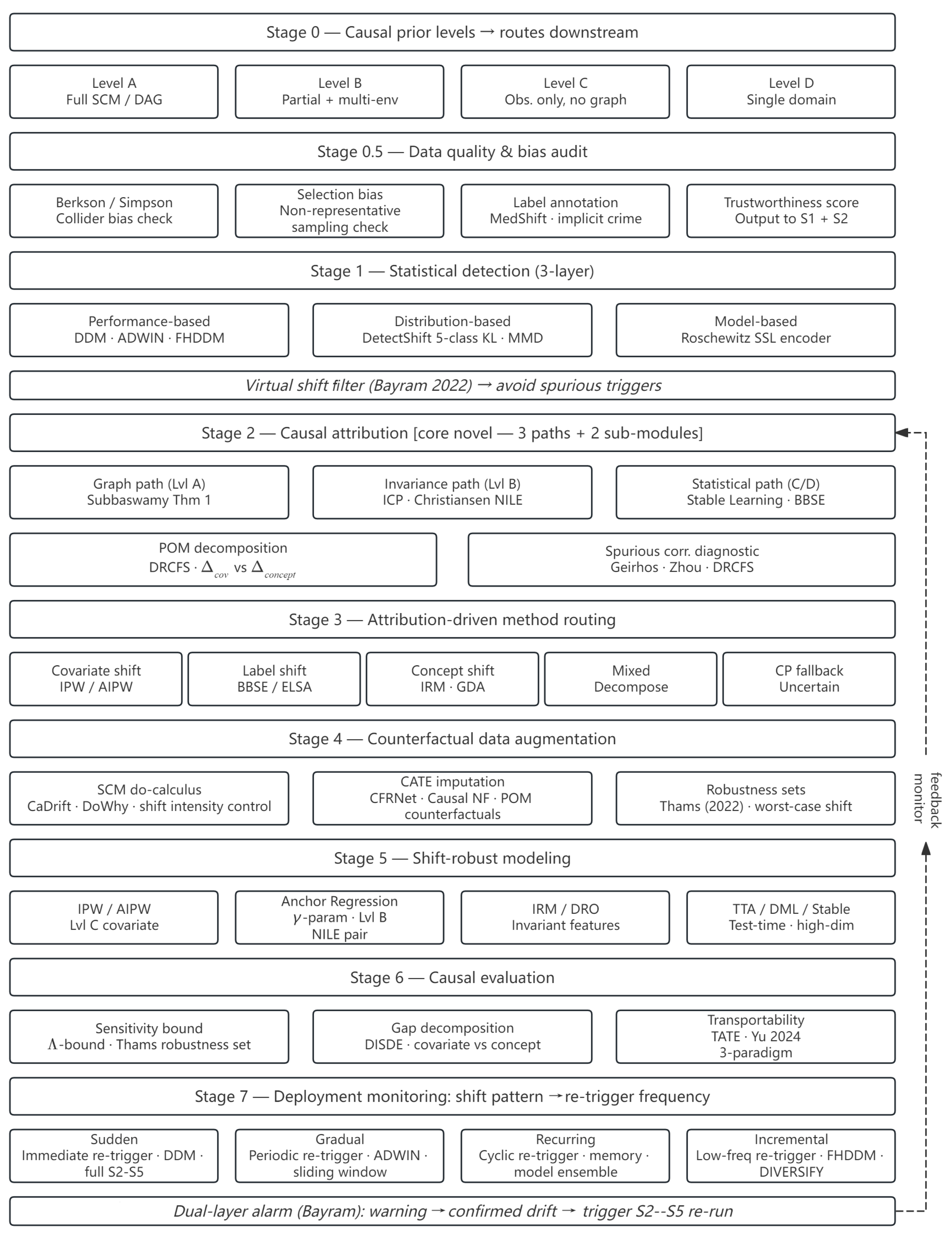
Table 1.
Causal knowledge grading system. Plugins not listed for a level are deactivated. “Env” denotes heterogeneous training environments; “IV” denotes instrumental variable availability; p denotes feature dimensionality.
Table 1.
Causal knowledge grading system. Plugins not listed for a level are deactivated. “Env” denotes heterogeneous training environments; “IV” denotes instrumental variable availability; p denotes feature dimensionality.
| Level | Available evidence | Active plugins | Attribution path |
|---|---|---|---|
| A | Full SCM or expert DAG | Graph, POM, Anchor | §3.2.1 |
| B | Multi-env data; IV optional; | Invariance, POM, Anchor | §3.2.2 |
| C | Single-domain observational; no graph | POM | §3.2.3 |
| D | Single-domain; high-dim () | None (Layer 1 only) | §3.2.3 |
Table 2.
Attribution-driven routing table. The dominant shift type and knowledge level jointly determine the primary adaptation strategy. CP = conformal prediction fallback.
Table 2.
Attribution-driven routing table. The dominant shift type and knowledge level jointly determine the primary adaptation strategy. CP = conformal prediction fallback.
| Dominant shift | Knowledge level | Primary strategy | Theoretical basis |
|---|---|---|---|
| Covariate | Any | IPW / AIPW / KMM | Sugiyama et al. [26] |
| Label | Any | BBSE / ELSA | Lipton et al. [27], Tian et al. [37] |
| Concept (mild) | A | GDA via removal | Subbaswamy et al. [14] |
| Concept (mild) | B | IRM / Anchor Regression | Arjovsky et al. [16], Rothenhäusler et al. [29] |
| Concept (severe) | A | GDA via removal | Subbaswamy et al. [14] Prop. 7 |
| Concept | C/D | Stable Learning + TTA | Cui and Athey [11], Wang et al. [28] |
| Mixed | A/B | Decompose via Eq. (2), stack | Peters et al. [23] |
| Mixed / uncertain | Any | CP fallback | Tibshirani et al. [30] |
Table 3.
Stage 2 attribution accuracy on the synthetic SCM (mean ± std, 3 seeds). Level A uses the known causal graph; Level C uses the POM statistical path. Stage 1 detects shift for all three variants (see text), causing Stage 2 to route to concept attribution in every case.
Table 3.
Stage 2 attribution accuracy on the synthetic SCM (mean ± std, 3 seeds). Level A uses the known causal graph; Level C uses the POM statistical path. Stage 1 detects shift for all three variants (see text), causing Stage 2 to route to concept attribution in every case.
| Shift variant | Level A | Level C |
|---|---|---|
| Covariate | ||
| Concept | ||
| Mixed |
Table 4.
OOD accuracy (%) and ID–OOD gap (%) on the three strong-shift benchmarks. Synthetic SCM: averaged over three shift variants and three seeds (, ). CMNIST: 60k train / 2k test, 392 pixel features. Camelyon17: ResNet-50 features (2,048 dims), 3k/1k patches. Bold: best OOD accuracy per dataset; underline: smallest gap.
Table 4.
OOD accuracy (%) and ID–OOD gap (%) on the three strong-shift benchmarks. Synthetic SCM: averaged over three shift variants and three seeds (, ). CMNIST: 60k train / 2k test, 392 pixel features. Camelyon17: ResNet-50 features (2,048 dims), 3k/1k patches. Bold: best OOD accuracy per dataset; underline: smallest gap.
| Synthetic SCM | CMNIST | Camelyon17 | ||||
|---|---|---|---|---|---|---|
| Method | OOD | OOD | OOD | |||
| ERM | 71.5 | 26.7 | 12.0 | 72.6 | 79.9 | 19.9 |
| IRM | 71.6 | 26.6 | 11.7 | 73.0 | 79.9 | 19.9 |
| CORAL | 72.5 | 25.1 | 12.0 | 72.6 | 77.0 | 22.8 |
| DetectShift+Best | 72.2 | 25.6 | 12.0 | 72.6 | 79.9 | 19.9 |
| CausalShift | 67.6 | 6.8 | 50.0 | 0.1 | 80.5 | 19.5 |
Table 7.
Ablation on the synthetic SCM (all variants, avg., 3 seeds). computed within each ablation run against a per-run ERM baseline. † Expected no-effect: audit passes on clean data; § Expected no-effect: CP fallback / POM do not alter routing on well-defined synthetic variants (see text).
Table 7.
Ablation on the synthetic SCM (all variants, avg., 3 seeds). computed within each ablation run against a per-run ERM baseline. † Expected no-effect: audit passes on clean data; § Expected no-effect: CP fallback / POM do not alter routing on well-defined synthetic variants (see text).
| Configuration | OOD | ||
|---|---|---|---|
| Full CausalShift (Level C/A) | 67.6 | 6.8 | 3.55 |
| − Stage 0.5 data audit† | 67.6 | 6.8 | 3.55 |
| − Causal plugins (Level D) | 66.3 | 30.5 | 0.80 |
| − CP fallback§ | 67.6 | 6.8 | 3.55 |
| − POM decomposition§ | 67.6 | 6.8 | 3.55 |
Disclaimer/Publisher’s Note: The statements, opinions and data contained in all publications are solely those of the individual author(s) and contributor(s) and not of MDPI and/or the editor(s). MDPI and/or the editor(s) disclaim responsibility for any injury to people or property resulting from any ideas, methods, instructions or products referred to in the content. |
© 2026 by the authors. Licensee MDPI, Basel, Switzerland. This article is an open access article distributed under the terms and conditions of the Creative Commons Attribution (CC BY) license (http://creativecommons.org/licenses/by/4.0/).
Copyright: This open access article is published under a Creative Commons CC BY 4.0 license, which permit the free download, distribution, and reuse, provided that the author and preprint are cited in any reuse.


