

Submitted:
09 June 2026
Posted:
10 June 2026
You are already at the latest version
Abstract
Stability of vehicles is one of the most important factors of safety. When assessing the conditions for the stability of the vehicle, on-road and off road vehicles differ in many perspectives, and because this, specific methods are needed to describe the stability conditions for terrain vehicles. In this paper, the aspects of off-road vehicle stability are assessed, terrain vehicle specific stability modeling methods are shown. After that, the LiDAR based terrain mapping technology and the measurement and remote sensing possibilities for the variables affecting the stability, both from the side of the vehicle and terrain, are introduced. At the end, field measurements conducted with a small scale remote controlled vehicle are presented.
Keywords:
off-road vehicle
; lidar
; vehicle stability
; terrain mapping
1. Introduction
Off-road mobility of vehicles is influenced by numerous factors, both from the side of the vehicle and terrain, and modeling methods for terrain vehicles should take into account both of these. While many different mobility models are accessible in the literature, most of them are created by assuming the presence of a driver, who can make manual corrections, and for this reason, these mobility models use a larger scale. However, for unmanned and autonomous vehicles, where no driver is present, the mobility model should be created with an accordingly small scale, so that the vehicle can avoid all obstacles based on the mobility model alone. In this paper, a mobility modeling method is presented, which aims to fulfill these criteria. The mobility model assesses the stability, obstacle negotiation capability, and the required traction and grip to determine the mobility through each part of the terrain. After the theoretical basis of the model is shown, laboratory and field experiments are conducted to measure the required parameters of the test vehicle, and a drone based surveying system is used to create a digital terrain map of the test terrain. At the end, field experiments are conducted on both a natural terrain section and artificial obstacle to experimentally validate the model.
2. Materials and Methods
2.1. Modeling of the Vehicle Stability
The stability for both on-road and off-road vehicles has two separate factors, and thus two cases to limit the mobility of vehicle on terrain. The roll and pitch stability of the vehicle limits the angle at which the vehicle can travel without a rollover occurring. The base geometrical criteria of a rollover is that the center of mass of the vehicle is positioned outside of the area circumscribed by the contact patch of the wheels. [1] This is affected, apart from the geometrical position of the vehicle, also by the shocks and vibration induced by the movement of the vehicle. [2] For on-road vehicles, a rollover can mostly occur as a result of an impact, as the vehicles normally travel on close to horizontal road surfaces. [3] However, for terrain vehicles, it is not unusual that the vehicles move to terrain surfaces which slope angle in itself can surpass, or at least be in the range of the rollover stability limit angle. For this reason, as for terrain vehicles the slope angle is usually a not negligible factor for rollover stability, a different approach is required for stability modeling. [4,5] While vibrations can cause a momentarily separation of the tire and the ground surface, assessing whether this separation results in an actual control of stability loss of the vehicle would be not feasible, for this reason, the loss of stability is considered to occur if a wheel loses contact with the ground due to the angle and vibrations of the vehicle [6].
In the following, the rollover stability modeling will be presented on a 2 dimensional model for the pitch angle, however, methods used for the roll stability are similar to this.
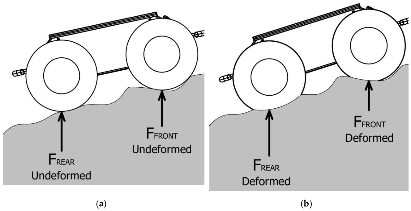
As it is shown in Figure 1, the basis for the stability is the pitch angle of the vehicle, which is both affected by the terrain surface, and the characteristic dimensions of the vehicle. Based on these values, a static pitch angle for the vehicle can be calculated at each point along the path of the vehicle, with basic geometrical methods. This static angle however, does not represent two important effects, the acceleration due to shocks and vibrations, and the change in the pitch angle due to the suspension displacement and wheel-soil deformation characteristics. However, both of these displacement values are calculated as function of the wheel / axle load, and this load is effected by the pitch angle due to the shift in the weight distribution between the wheels. [7] For this reason, an iterative process could be used to calculate the suspension and wheel-soil displacement values. However, to simplify the calculations, an approximation was made to calculate these values based on the wheel load distribution of the undeformed case, considering that the displacement is relatively low compared to the height difference due to the slope angle.
Figure 1.
Stability of the vehicle; (a) Stable position; (b) Unstable position.
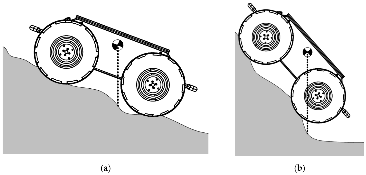
Figure 2.
Change in the wheel load distribution; (a) Undeformed state; (b) Deformed state.
The tire-soil deformation characteristics are usually described with rheological models, including a viscoelastic [8,9] or viscoelastoplastic [10] rheological models. As the test vehicle used in this experiment has a relatively low top speed, it was considered that the viscous part of these models is negligible, and an elastoplastic serial model is used, shown on Figure 3. The parameter identification for this model was carried out by laboratory and field measurements with the test vehicle. As the ground contact surface is not planar, instead of single arithmetical equations or rheological models, which are often used in simplified cases [11], a parallel element model was used, which means that the deformation is characterized by multiple, but independently acting elements. [12]
After the pitch angle is actualized with the suspension displacement and wheel-soil deformation, this static pitch angle is compared to the stability limit angle of the vehicle. For easier comparison, instead of displaying the limit angle in degrees or radians, the actual pitch angle is expressed as a percentage of the limit.
In a static case, this limit would be 100%, or 1, if expressed as a decimal value. This gives a correct assessment of the stability if the vehicle travels at a very slow speed, where dynamic effects are negligible. However, this rollover stability limit needs to be adjusted based on the dynamic vibrations at higher speeds.
The other important aspect of the vehicle safety and stability is the available grip or traction. For terrain vehicles, the available grip is usually limited by the shear strength of the soil, and cannot be expressed as a simple friction coefficient. For this reason, the traction values were obtained using field measurements with the model vehicle. For the safety assessment, the available traction values should be compared to the required traction for a safe traverse. This means that the vehicle needs to be able to extort enough traction to surpass all resistances, and have enough traction for to safely conduct an emergency braking at any point of the path. [13,14] The motion of the vehicle can be described with the equations
where Fa is the acceleration force, Ft is the traction, R is the rolling resistance, Fe is the gravitational resistance, f is the rolling resistance coefficient, g is the gravitational coefficient, m is the vehicles mass, α is the slope angle.
The main resistances for a terrain vehicle are the rolling resistance and the elevational resistance. The elevational resistance is obtained from the pitch angle of the vehicle, and the rolling resistance coefficient is measured. The traction values are obtained from the measurements presented in the next section.
2.2. Vehicle Parameter Measurements
The parameters of the vehicle were measured in laboratory and field conditions. The measured parameters are:
- Weight and center of gravity position
- Moment of inertia
- Traction on different soil conditions
2.2.1. Center of Gravity Measurement
The measurement was conducted using a conventional method by wheel scales, tilting the vehicle along the roll and pitch axes [15] as it is shown in Figure 4. The wheel loads were measured both in a horizontal and tilted positions. The measurement results are shown in Table 1.
Based on the measurements, the position of the center of gravity is obtained by the following equations. Longitudinal position is
where xCG is longitudinal coordinate of the center of gravity, L is the wheelbase, F1 and F2 are the wheel / axle loads in the vertical measurement position.
The transversal position could be calculated with the same method. However, based on the measurements, it was examined that due to the symmetrical build of the vehicle, it is approximately at the symmetry plane of the chassis, so no numerical calculations were needed.
Equation of the vertical position is
where hCG is the vertical coordinate of the center of gravity, F3 and F4 are the wheel / axle loads in the tilted position, H is the platform height, R is the wheel radius.
2.2.2. Moment of Inertia Measurement
The moment of inertia of a vehicle can be measured with multiple methods. In the conventional vehicle dynamic measurements, the moment of inertia is usually measured by bringing the vehicle into oscillation, either using a spring-loaded testbed [17], or the vehicles own suspension [18]. However in this experiment, considering the small scale of the vehicle, the moment of inertia is measured based on methods used for smaller rigid bodies outside of the vehicle technology [19] the gravitational acceleration, while pivoting the vehicle around one of the axes, as shown on Figure 7.
During the measurement, the wheel is disengaged and is in a free rotating state, which means that the center of rotation is on the wheel axis. From the gravitational acceleration, the moment of inertia is derived from the standard equation of the angular acceleration [20], obtained using the following formula
where M is the gravitational moment action on the chassis, JK is the moment of inertia on the wheel axis, β is the angular acceleration, s is the center of gravity position, J is the moment of inertia on the axis through the center of gravity.
Figure 8 shows a measured dataset. On the graph, the constant value of the acceleration due to gravity can be clearly seen.
In total, 6 measurements were conducted. For each measurement, 2 accelerometers were used. The average of these 2 values were considered for the calculations, these values can be seen in Table 2.
2.2.3. Traction Measurement
The traction of the vehicle was measured under static conditions. The traction was measured using a force inducer through a towing strap. The measurements were conducted on soils with different density, and on soil covered with vegetation, and with different payloads on the vehicle. The tire pressure was also considered to be changed during the measurements, but based on the pilot measurement is was assumed that its effect on the traction is negligible. The measurement setup is seen in Figure 9 and Figure 10.
With each load and soil type, the traction was measured 3 times, which is seen on Figure 11. On the graph, the intervals of the static and dynamic friction. For the available traction value, the average of the dynamic frictional interval was calculated.
2.3. Setup for Validation Measurements
The experimental measurements were conducted in a test field on the Hungarian University of Agriculture. Of the terrain, a set of obstacles fitting the scale of the vehicle was built, which is shown in Figure 12 and Figure 13.
For the tests, the vehicle was outfitted with an array of sensors, which is shown on Figure 14.
The position of the vehicle was obtained using a stereo RTK/GNSS system, which gives both the position and orientation of the vehicle. The positional data was collected with a resolution of 10-7 ° (approximately 1 cm) on both the longitude and latitude coordinates independently, and the accuracy of the measurement was between 3-5 cm. The orientation was also measured using an inertial measurement unit (IMU). During the tests, the traction (obtained from the torque of the motors) was logged by the vehicles control unit as a function of time. These values were correlated to the position of the vehicle based on the timestamps. The acceleration at each wheel was measured using the same measurement sensors introduced in the section „Moment of inertia measurement”
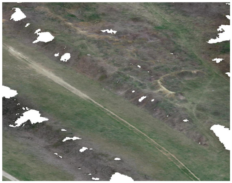
2.4. LiDAR Based Terrain Mapping
For terrain mapping purposes the most applied method is unmanned aerial vehicle (UAV) based remote sensing. Two sensing techniques are used by devices mounted on UAVs. Photogrammetry relies on capturing high resolution images (usually RGB images) with low distortion optics cameras with appropriate overlap between neighbouring images. Knowing the precise geolocation of the UAV a software identifies matching points between images taken at different locations and determines their spatial coordinates through triangulation. As a result, the software tool can generate a digital terrain model in the form of a point cloud from the series of plain images. This method is quick, does not require special sensory tool besides a good quality camera, might result in relatively good resolution point cloud and directly provides RGB colour information assigned to each point. However, it has drawbacks due to the influencing effect of illumination of the surface and shading effects and has limited accuracy of 3–6 cm of uncertainty in estimating point coordinates. LiDAR provides an alternative UAV-based surveying method. As an active sensor, it determines the distance to surface points by measuring the time of flight of emitted laser pulses. LiDAR can rapidly generate dense point clouds comparable to those from photogrammetry, and can also record multiple returns from a single pulse, enabling partial detection of vegetation-covered surfaces.
Accurate positioning and orientation of the UAV and its sensors are essential for both photogrammetric and LiDAR-based surveying. These data are usually acquired from centimetre accuracy RTK corrected GNSS services combined with acceleration, angular velocity and geomagnetic field strength measurement from onboard inertial measuring units (IMUs). The absolute accuracy of positioning the point cloud can be improved further by applying ground control points of known positions around the surveying area used as references for calibration.
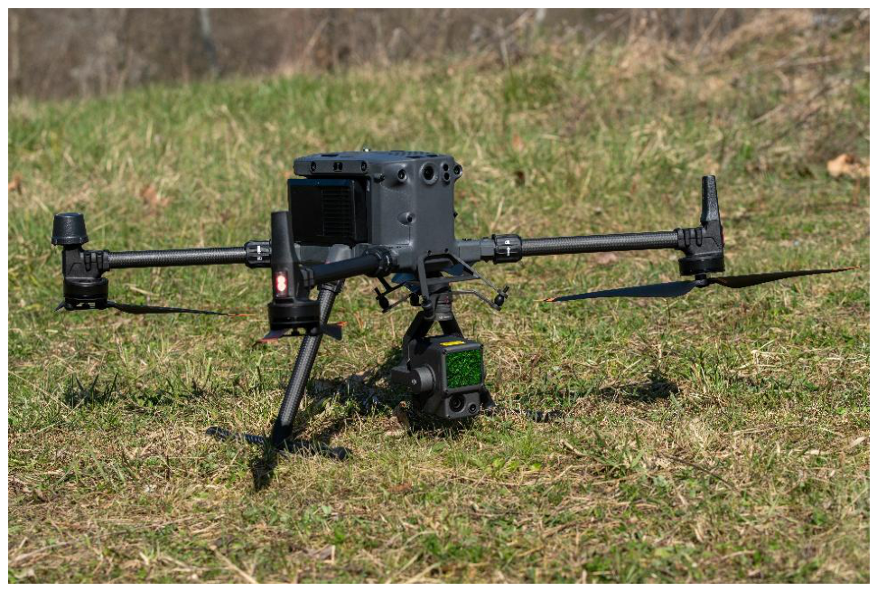
In surveying the MATE test field for mobility mapping purposes, a DJI Matrice 350 RTK quadcopter UAV equipped with a DJI Zenmuse L1 LiDAR scanner was applied for airborne terrain mapping. Main specifications of the LiDAR are the following:
• maximum sensing range 450 m,
• single or triple return detection modes,
• point rate: 240000 points/s (single), 480000 point/s (triple),
• standard uncertainty @ 50 m: 10 cm (horizontal), 5 cm (vertical),
• real time depth based, distance based, reflectance based or visible camera RGB camera based colouring modes,
• field of view: 70.4° (horizontal) x 77.2°(vertical) with non-repetitive scanning pattern or 70.4° (horizontal) x 4.5° (vertical) with repetitive scanning pattern,
• supplementary RGB mapping camera resolution: 20 MP (5472 x 3078 or 4864 x 3648 or 5472 x 3648 depending on aspect ratio setting).
Figure 15.
Drone-borne measurement system.
Measurement setup is supplemented with an Emlid Reach RS2+ type GNSS receiver operating as local RTK base station to provide correction signal for UAV accurate positioning. The base station was set up on a previously surveyed ground reference point close to the testing area and had access to Hungarian network RTK service MAXI-NET 2.0 to improve absolute positioning. The UAV flew an ortho-mapping mission covering approximately 15,000 m². Key planning parameters were:
• flight altitude: 38 m, relative to take-off point (AGL),
• elevation optimization enabled,
• ground speed: 3.6 m/s,
• point density: 693 points/m2
• triple return mode,
• RGB camera ground sampling distance (GSD): 1.04 cm/px,
• side overlap ratio - LiDAR: 20%, - RGB camera: 38%,
• frontal overlap ratio (RGB camera): 70%.
The recorded point cloud was processed in DJI Terra 5.1.1 software. The raw point cloud data were imported to the software where applying the proper settings a raster grid with a 10 cm vertical resolution was created.
Figure 16.
Point cloud obtained by LiDAR mapping.
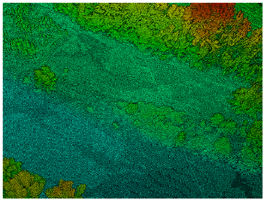
Figure 17.
Rasterized digital terrain model of the test area.
3. Results
During the measurement, data was collected at approximately 12000 data points. In the following section, the results are shown for the vehicle traversing on a slope type obstacle. On Figure 18., the comparison of the predicted and measured stability index is shown. As discussed earlier, by using this decimal value, the limit of vehicle stability is 1. As it can be seen on the graph, in the range of the stability index below 1, the prediction accurately represents the measured values. We can see a significant difference at the beginning, approximately between 0 and 2 seconds. This can be explained by the initial acceleration of the vehicle from a static position, as this large longitudinal acceleration influences the inertial measurement.
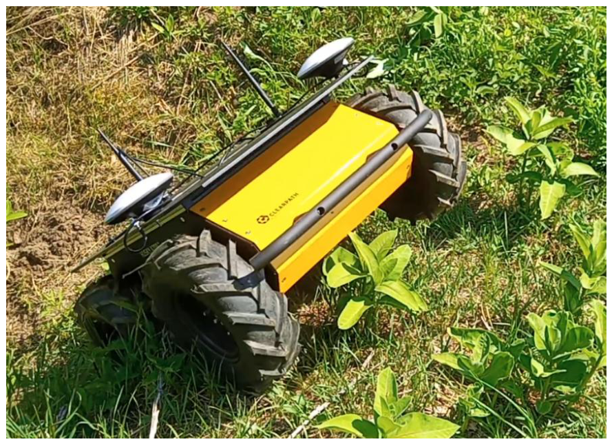
The loss of stability can be seen at the graph, when the value of the stability index surpasses the value 1, at approximately 11 seconds. This is the point of stability loss, which is pictured in Figure 20. After this point, the vehicle rolls over uncontrollably, that explains why the predicted and measured values after this point are diverging.
Figure 19.
Stable position of the vehicle during the tests.
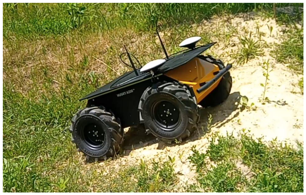
Figure 20.
Vehicle at the point of stability loss.
4. Discussion
The accuracy of the stability prediction can be described by conventional statistic methods. However, besides the mathematical accuracy, the differentiation between false negatives and positives is very important in this case. A false positive error would mean that the vehicle will be predicted to be stable and safe to traverse through an obstacle according to the model, while in reality a loss stability will occur, which can lead to material, and even bodily harm. To the contrary, a false negative prediction only means that the vehicle will be restricted from a route that could be physically traversable, which could make route planning and operation suboptimal, but does not negatively affect safety. The error histogram of the model is shown on Figure 21. It can be seen that the model is biased towards the side of false negatives, which is favorable from a safety perspective. False positive predictions still occur, but these can be mitigated by introducing a safety factor, which shifts all errors into the false negative field, although this also introduces the aforementioned suboptimality.
Funding
This research was supported by the Ministry of Culture and Innovation and the National Re-search, Development and Innovation Office within the Cooperative Technologies National La-boratory of Hungary (Grant No. 2022-2.1.1-NL-2022-00012), Project no. 2024-1.2.5-TÉT-2024-00075 and the Cooperative Doctoral Programme.
Data Availability Statement
We encourage all authors of articles published in MDPI journals to share their research data. In this section, please provide details regarding where data supporting reported results can be found, including links to publicly archived datasets analyzed or generated during the study. Where no new data were created, or where data is unavailable due to privacy or ethical restrictions, a statement is still required. Suggested Data Availability Statements are available in section “MDPI Research Data Policies” at https://www.mdpi.com/ethics.
Conflicts of Interest
The authors declare no conflicts of interest. The funders had no role in the design of the study; in the collection, analyses, or interpretation of data; in the writing of the manuscript; or in the decision to publish the results.
References
- Laib, L. 2002. Terepen Mozgó Járművek; Szaktudás Kiadó Ház, Budapest, Hungary.
- Taghavifar, H. & Mardani, A. 2017. Off-road vehicle dynamics. Studies in Systems, Decision and Control, 70, 37.
- Cooperrider, N.K. et al. 1990. Testing and analysis of vehicle rollover behavior. SAE Technical Paper No. 900366.
- Mann, M.P. & Shiller, Z. 2006. Dynamic stability of off-road vehicles: a geometric approach. Proceedings 2006 IEEE International Conference on Robotics and Automation, 2006. ICRA 2006., Orlando, FL, USA, 2006, pp. 3705-3710. [CrossRef]
- Liu, J. & Ayers, P.D. 1999. Off-road vehicle rollover and field testing of stability index. Journal of agricultural safety and health, 5(1), 59.
- Lee, D. et al. 2023. Analysis of overturning stability of small off-road vehicle. Journal of Biosystems Engineering, 48(3), 309-318.
- Pytka, J. 2010. Experimental research on stability of an off-road vehicle on deformable surfaces. SAE 2010 Commercial Vehicle Engineering Congress, Technical Paper.
- Yin, Y. et al. 2016. A roll stability performance measure for off-road vehicles. Journal of Terramechanics, 64, 58-68.
- Józefiak, K. & Zbiciak, A. 2017. Secondary consolidation modelling by using rheological schemes. MATEC Web Conf. 2017, 117, 00069.
- Komamura, F. & Huang, R.J. 1974. New rheological model for soil behavior. J. Geotech. Eng. Div. 1974, 100, 807–824.
- Swamy, V. S. et al. 2023. Review of modeling and validation techniques for tire-deformable soil interactions. Journal of Terramechanics, 109, 73-92.
- Feng, H. et al. 2021. Finite element simulation of the viscoelastic behavior of elastomers under finite deformation with consideration of nonlinear material viscosity. Acta Mechanica, 232(10), 4111-4132.
- Gao, Y. 2012. Vehicle Dynamics and Performance. Meyers, R.A. Encyclopedia of Sustainability Science and Technology. Springer, New York, NY. [CrossRef]
- Wong, J.Y. 2022. Theory of ground vehicles. John Wiley & Sons.
- Botha, T.R. & Els, P.S. 2019. Vehicle centre of mass, roll-centre and pitch-centre height estimation. International Journal of Vehicle Systems Modelling and Testing, 13(4), 319-339.
- Ayers, P. et al. 2018. Stability analysis of agricultural off-road vehicles. Journal of agricultural safety and health, 24(3), 167-182.
- Uys, P.E. et al. 2006. Experimental Determination of Moments of Inertia for an Off-Road Vehicle in a Regular Engineering Laboratory. International Journal of Mechanical Engineering Education. 2006;34(4):291-314. [CrossRef]
- MacInnis, D. et al. 1997. A Comparison of Moment of Inertia Estimation Techniques for Vehicle Dynamics Simulation. SAE Technical Paper 970951, 1997. [CrossRef]
- Hinrichsen, F.P. 2022. A Simple Moment of Inertia Measurement. The Physics Teacher, 1 April 2022; 60 (4): 292–295. [CrossRef]
- Kozmann, Gy. 1976. Műszaki lengéstan, Tankönyvkiadó, Budapest.
Figure 3.
Rheological model of tire-soil deformation.
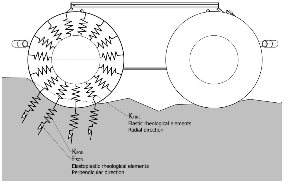
Figure 4.
Center of gravity measurement.
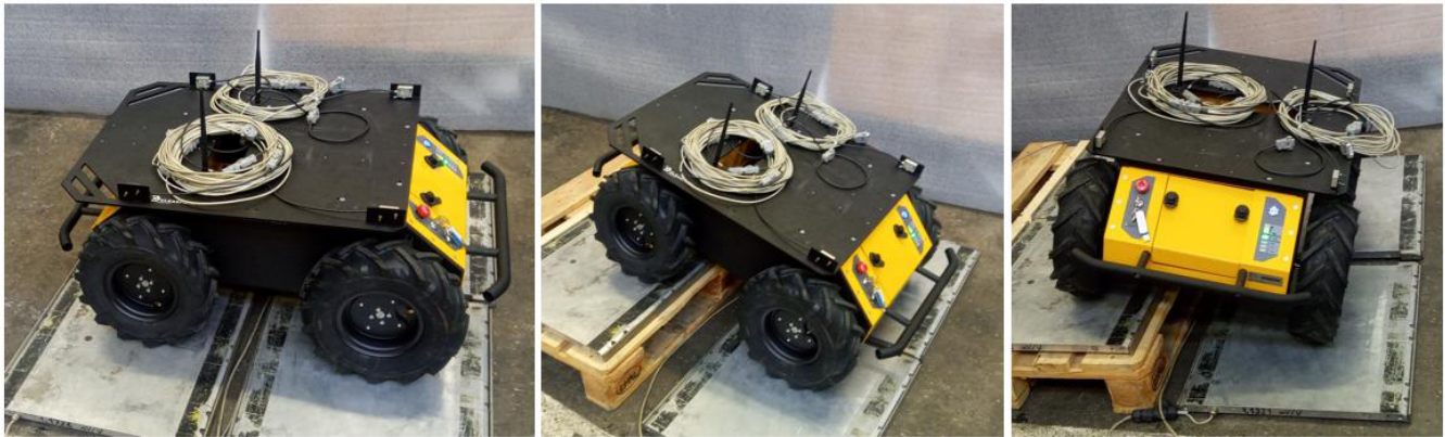
Figure 5.
Center of gravity position on test vehicle.
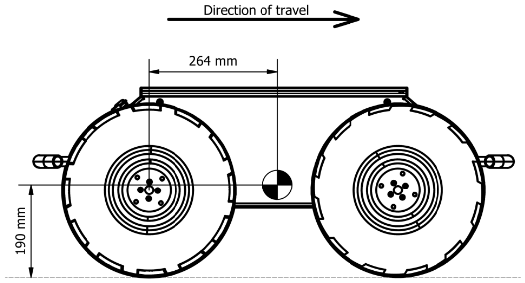
Figure 6.
Longitudinal stability limits of test vehicle.
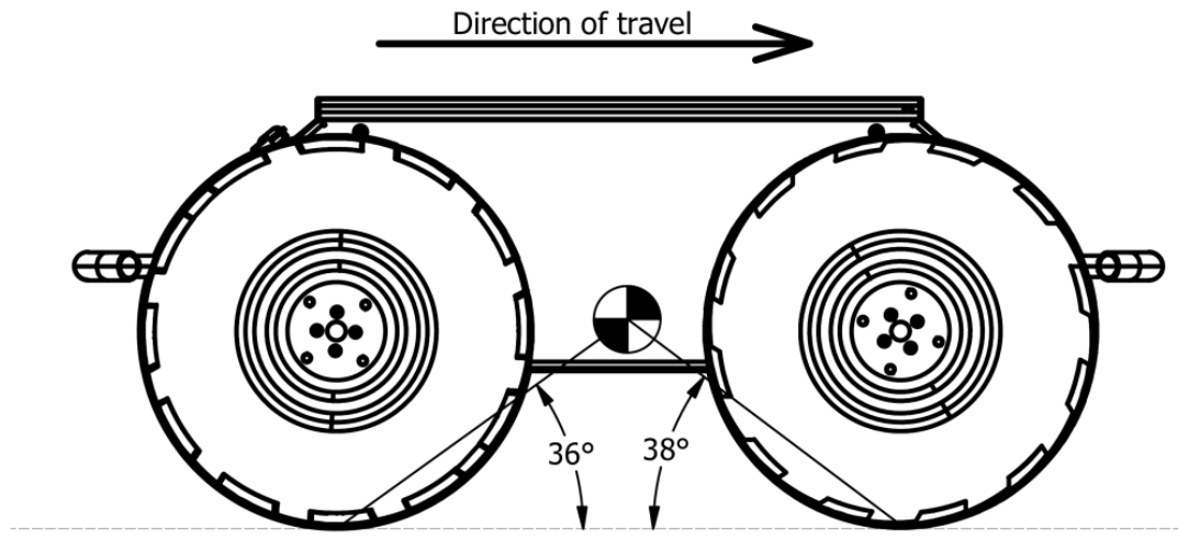
Figure 7.
Moment of inertia measurement.
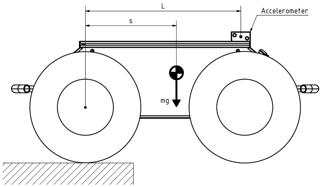
Figure 8.
Measured acceleration values.
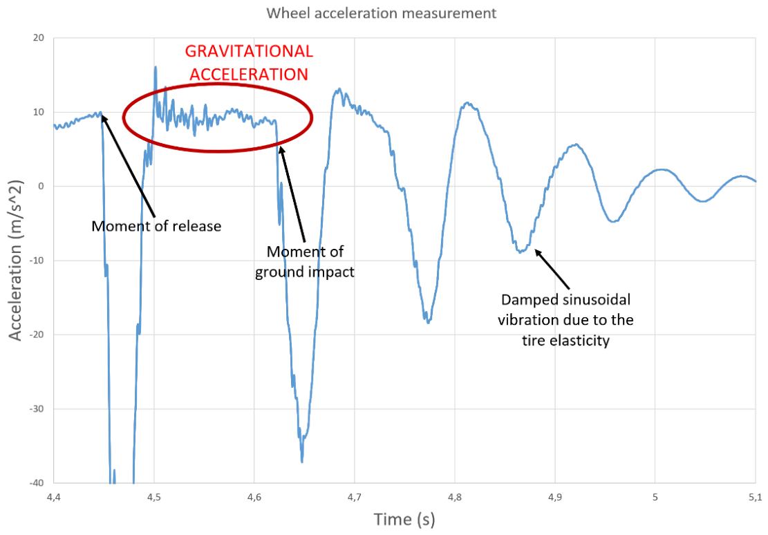
Figure 9.
Traction measurement in fixed position.
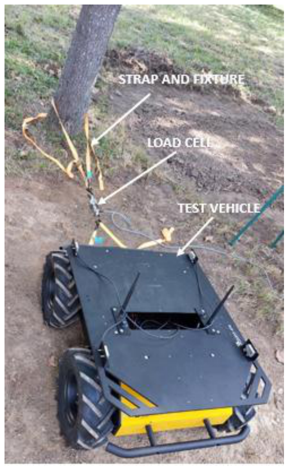
Figure 10.
Measurement setup for traction measurement.
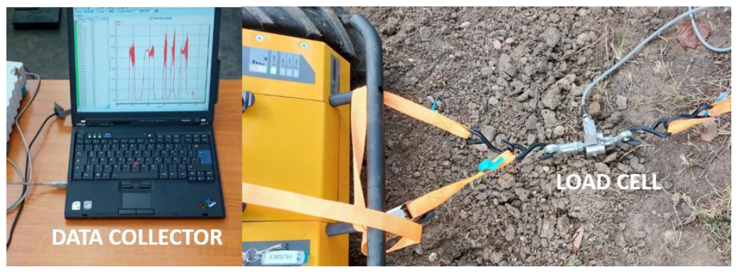
Figure 11.
Results of traction measurement (20 kg load, loose soil).
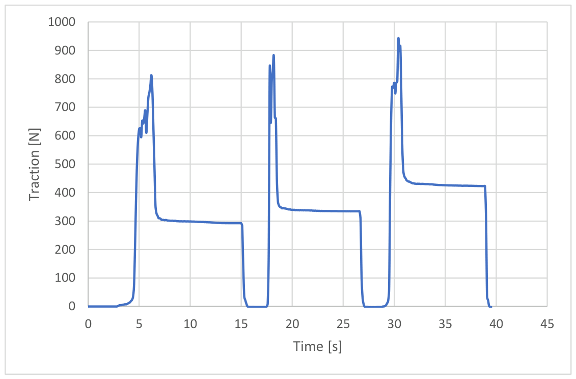
Figure 12.
Aerial view of test area.
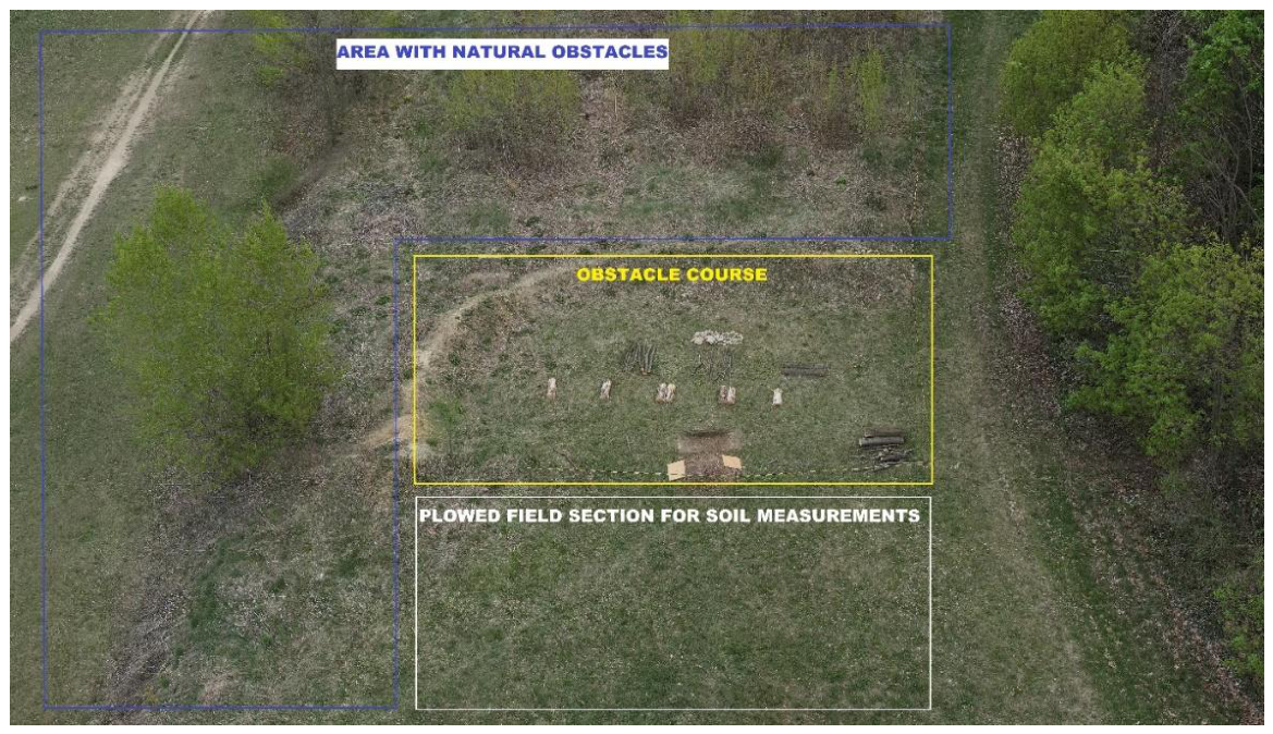
Figure 13.
Obstacle course on the test area.
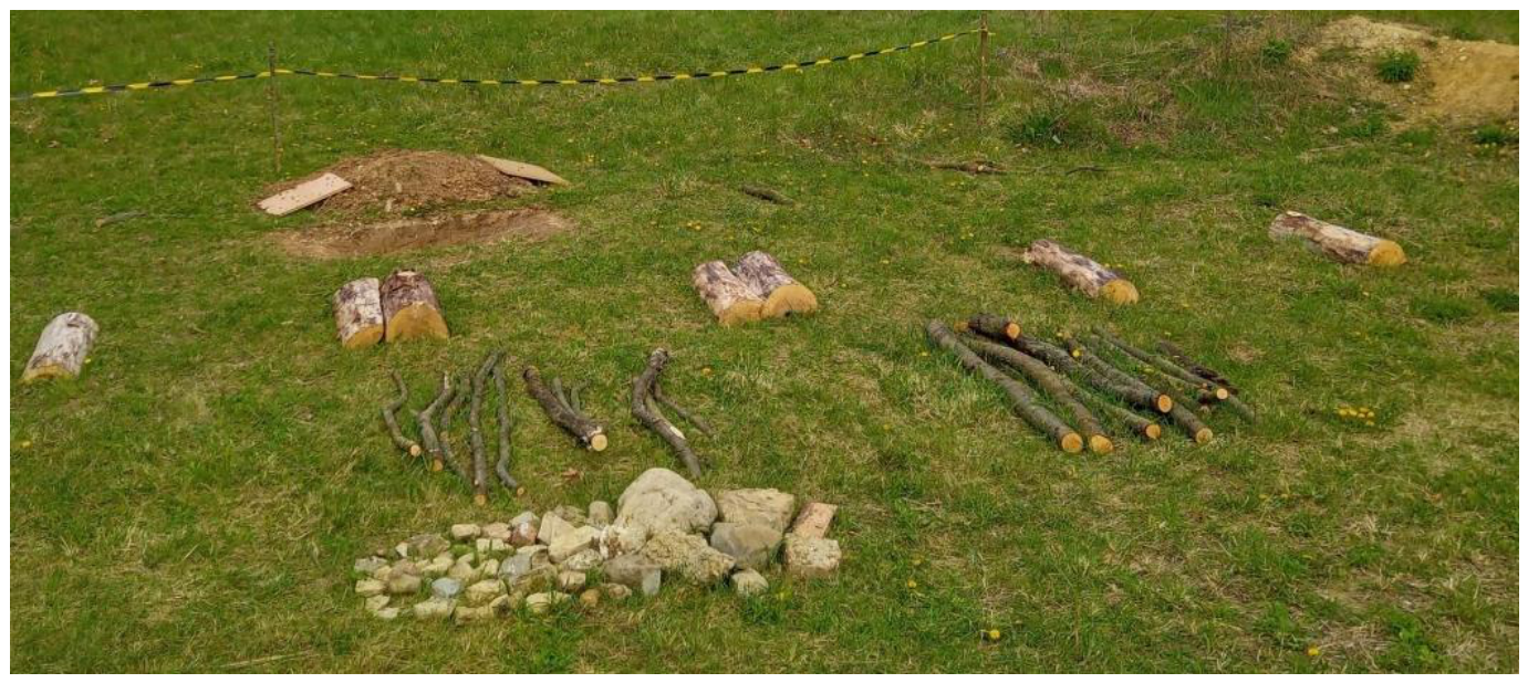
Figure 14.
Test vehicle outfitted with sensor array.
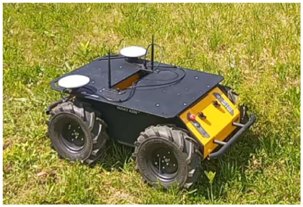
Figure 18.
Results of the validation measurement.
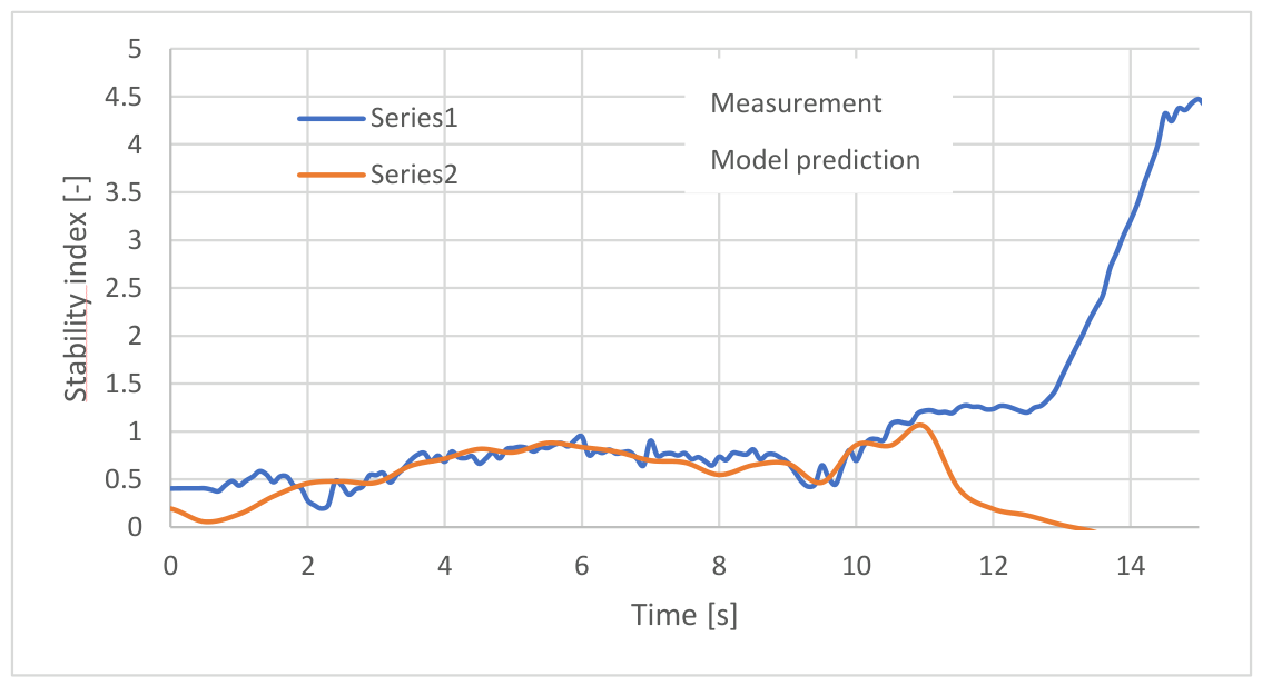
Figure 21.
Error histogram of the stability model.
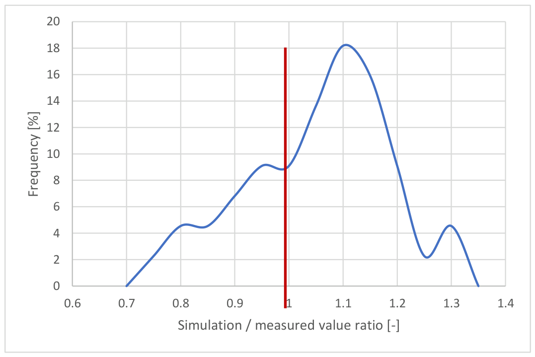

Table 1.
Wheel load measurement results.
| Axle load (kg) | Wheel lift height (mm) | ||
| Front | Rear | Front | Rear |
| 26.1 | 24.5 | 0 | 0 |
| 35.6 | 15 | 0 | 155 |
| 35 | 15.6 | 250 | 0 |
Table 2.
Moment of inertia measurement results.
| Measurement | a (m/s2) | J (kgm2) |
| 1 | 9.39 | 3.67 |
| 2 | 9.33 | 3.71 |
| 3 | 9.24 | 3.78 |
| 4 | 9.20 | 3.81 |
| 5 | 9.35 | 3.69 |
| 6 | 9.45 | 3.62 |
Disclaimer/Publisher’s Note: The statements, opinions and data contained in all publications are solely those of the individual author(s) and contributor(s) and not of MDPI and/or the editor(s). MDPI and/or the editor(s) disclaim responsibility for any injury to people or property resulting from any ideas, methods, instructions or products referred to in the content. |
© 2026 by the authors. Licensee MDPI, Basel, Switzerland. This article is an open access article distributed under the terms and conditions of the Creative Commons Attribution (CC BY) license (http://creativecommons.org/licenses/by/4.0/).
Copyright: This open access article is published under a Creative Commons CC BY 4.0 license, which permit the free download, distribution, and reuse, provided that the author and preprint are cited in any reuse.


