

Submitted:
10 June 2026
Posted:
16 June 2026
You are already at the latest version
Abstract
We give a comprehensive finite-field realisation of the Riemann Hypothesis within the Finite Ring Cosmology framework, where arithmetic is carried by a local observer shell operating on a large but ultimately finite relational algebraic substrate. The Riemann zero heights are realised as the finite spectrum of the scale-evolution operator \(\hat{H}=-i(x\partial_x+1/2)\) and are computed from the primes alone: the von Mangoldt comb drives a secular condition and an explicit matrix whose eigenvalues recover the heights to \(4\times10^{-5}\), with \(\zeta\) never evaluated. On the shell the half-turn 1/2 is three things at once: the self-dual locus \(\mathrm{Tr}=1\), the symmetrizer that makes the operator self-adjoint, and the critical real part. The real part of a zero is therefore fixed at \(1/2\) by construction, for the same reason that primes are natural numbers fixed to the real line: both live where the observer and Carrier frames agree. The Riemann Hypothesis reduces to a single clause, the completeness of this spectrum for the prime vector. Completeness is a \(\Pi^0_1\) statement, a single unbounded quantifier over heights: \emph{no zero off the line, ever}. The finite totality closes the domain of that quantifier. Below the observer horizon \(\Omega^{1/4}\sim10^{30}\) the clause is decidable height by height, and is verified to \(3\times10^{12}\). Between \(\Omega^{1/4}\) and the coherence horizon \(\sqrt\Omega\sim10^{61}\) it is bounded but unresolvable in any finite observer frame. Beyond \(\sqrt\Omega\) the height chart wraps onto the sub-horizon cycle, so the trans-horizon region is identified, not populated. Two premises carry this closure: the finitude of the totality, concluded by a formal reductio ad absurdum argument against completed infinity, currently under review, and the frame-covariance of the height chart. The entire content of the hypothesis is then the bounded completeness clause below the horizon: relocated, not removed. The generalized hypothesis reduces on the same footing through the \(\chi\)-twist. The Davenport-Heilbronn function, which lacks an Euler product, carries off-line zeros exactly as the construction predicts; we demonstrate this with a positive control. The paper closes with the physical reading of the construction, from the cosmological to the quantum end of the observable range.
Keywords:
riemann hypothesis
; finite fields
; zeta function
; finite ring continuum
; Hilbert-Pólya theory
; spectral realization
; prime-counting function
; von Mangoldt function
; dilation operator
; dirichlet L-functions
; companion matrices
1. Introduction
The nontrivial zeros of the Riemann zeta function lie, conjecturally, on the line . This paper gives a finite realisation of that hypothesis in the Finite Ring Cosmology (FRC) that posits the existence of a large but ultimately finite algebraic substrate. The framework rests on a formal reductio ad absurdum argument against completed infinity [1]; its conclusion — the finiteness of the totality — enters here as a stated premise, and what is derived from it is not the hypothesis itself but its reduction: the quantifier over heights closes at the coherence horizon, leaving a bounded completeness clause as the hypothesis’s entire content (Section 10.3). In this framework, the realised zeros are the spectrum of an explicit self-adjoint operator: the scale-evolution generator of the multiplicative line. This operator is universal; the primes enter through its trace formula, the prime-counting reconstruction. Its spectrum is therefore computed from the prime side, with never evaluated, in three forms: a spectral density, the discrete eigenvalues of a secular condition, and the roots of an explicit companion matrix with a self-adjoint Jacobi realisation. The half-turn places those modes on the self-dual line by construction.
The placement on is a construction identity at each finite shell, so the realised spectrum is on-line by construction; this is the unconditional content. The Riemann Hypothesis is the further claim that the on-line spectrum is complete for the prime vector — the faithfulness of the de-framing, the finite Hilbert–Pólya criterion. The construction reduces the universal hypothesis to a single, precisely located object: the reconstruction at zero leak, where the Subject and Carrier grids coincide everywhere, realisable only in the Carrier’s own frame and in no nested Subject shell. At each finite shell the result is quasi-stable — the hypothesis on the agreement loci, per height, with a residual leak. The hypothesis is ; with the Carrier finite (the reductio of [1]) the universal quantifier over heights is closed at the coherence horizon, leaving a bounded statement — verifiable below the horizon, the chart wrapping above it. The framework establishes the reduction and the quasi-stable verification; it does not occupy the closing frame. We first place the construction among existing spectral approaches to the hypothesis, then summarise the framework on which it builds.
1.1. The Spectral Approach and Prior Work
Since Riemann’s memoir [2] the conjecture that the nontrivial zeros of lie on has organised much of analytic number theory; standard accounts and surveys include [3,4,5,6,7]. Unconditionally a positive proportion of zeros is known to lie on the line — infinitely many by Hardy [8], more than a third by Levinson [9], more than two fifths by Conrey [10] — and large-scale computation has placed enormous initial segments on it [11], yet the hypothesis itself remains open.
The organising structural idea is the Hilbert–Pólya conjecture: that the zero ordinates are the spectrum of a self-adjoint operator, so that reality of the spectrum forces . Selberg’s trace formula [12], in which the lengths of closed geodesics and the eigenvalues of the Laplacian satisfy a duality formally identical to the explicit formula relating primes and zeros [13,14], furnishes a setting in which precisely such a spectral interpretation holds. Montgomery’s pair-correlation conjecture [15], with Dyson’s observation that it coincides with the Gaussian unitary ensemble, bound the local statistics of the zeros to random-matrix theory [16]. This was confirmed numerically by Odlyzko [11], extended to higher correlations and to general L-functions by Rudnick and Sarnak [17], organised by symmetry type by Katz and Sarnak [18,19], and connected to the moments of through the characteristic polynomials of random unitary matrices by Keating and Snaith [20].
A number of explicit operators have been proposed for this conjectural spectrum. Berry and Keating revived the classical Hamiltonian , whose semiclassical level count reproduces the Riemann–von Mangoldt density [21]. Connes recast the problem as a trace formula on the adèle class space, the zeros appearing as an absorption spectrum [22]. Sierra and Townsend realised the same dilation dynamics as the lowest Landau level of a charged particle [23]. Bender, Brody, and Müller exhibited a -symmetric operator formally vanishing at the zeros [24]. De Branges pursued the hypothesis through Hilbert spaces of entire functions [25], and Lapidus developed a fractal-string and noncommutative-geometric formulation [26]. The physical side of these programmes is surveyed by Schumayer and Hutchinson [27]. They share one unresolved difficulty — producing a single operator that is provably self-adjoint and whose spectrum is provably the zero set — which is among the obstructions this paper isolates rather than claims to remove.
The decisive piece of context is the function-field analogue, in which the Riemann hypothesis is a theorem. For the zeta functions of curves and varieties over finite fields the zeros lie on the critical line because they are eigenvalues of the Frobenius endomorphism acting on cohomology — proved by Weil for curves [28] and by Deligne in general [29], with the arithmetic of function fields developed in [30]. That the one unconditional realisation of the hypothesis is over a finite field, with the spectral object the Frobenius of a finite structure, is a direct motivation for seeking a finite-field substrate for the classical case.
The bar any such account must clear is set by the Davenport–Heilbronn function [31]: a Dirichlet series with a Riemann-type functional equation but no Euler product, which has infinitely many zeros off the critical line. Functional symmetry alone therefore cannot force the line, and any account that places every zero there by fiat is refuted at once. The present work belongs to the spectral family above: it realises the zeros as the spectrum of the dilation generator, computed from the prime side. It differs in its substrate. The construction is built on the finite relational shell of the Finite Ring Cosmology [32,33,34], where the critical line is the self-dual locus of a single symmetry-complete shell. There the Davenport–Heilbronn dichotomy reappears as the presence or absence of a single Euler-product structure.
1.2. The Finite-Ring Framework
The FRC framework — Finite Ring Continuum in its mathematical layer [32,33], Finite Ring Cosmology in the physical reading this paper adopts; the acronym is shared — reconstructs arithmetic over a finite prime field without a completed infinity: the labels 0 (position), 1 (scale), and the imaginary unit are not absolute marks on the field but frame data an observer assigns [32]. Fixing an affine frame makes a framed finite field, in which every algebraic identity is frame-covariant. The classical continuum is recovered only as a degenerate idealisation of the scale-periodic framed-rational refinement the shell already carries. This is the finitist reading, developed for physics by Lev [35,36] and for analysis by Zeilberger [37], on which the continuum is a degenerate case of a more fundamental finite mathematics. Throughout the paper the framework is used as a method: a finite apparatus for computing and characterizing the zeros. Its elevation from method to reduction — bounding the hypothesis by the finite totality, with no completed continuum standing apart from the shell — is a separate step (Section 10.3).
In the symmetry-complete regime the multiplicative group is cyclic of order and carries a genuine quarter-turn, so the affine frame extends to an extended affine frame by adjoining a phase chart [33]. Its primitive datum is a generator–turn pair: a primitive phase generator, which steps through the longitudes , and the oriented quarter-turn, an oriented square root of (). The exponential unit — the finite role of Euler’s e — is the quarter-turn transform of the generator,
relating the rotational generator (phase) to the exponential scale base. With this datum the shell carries the finite Euler identities
the finite form of , in which carry the structural roles of [33].
Remark 1.1
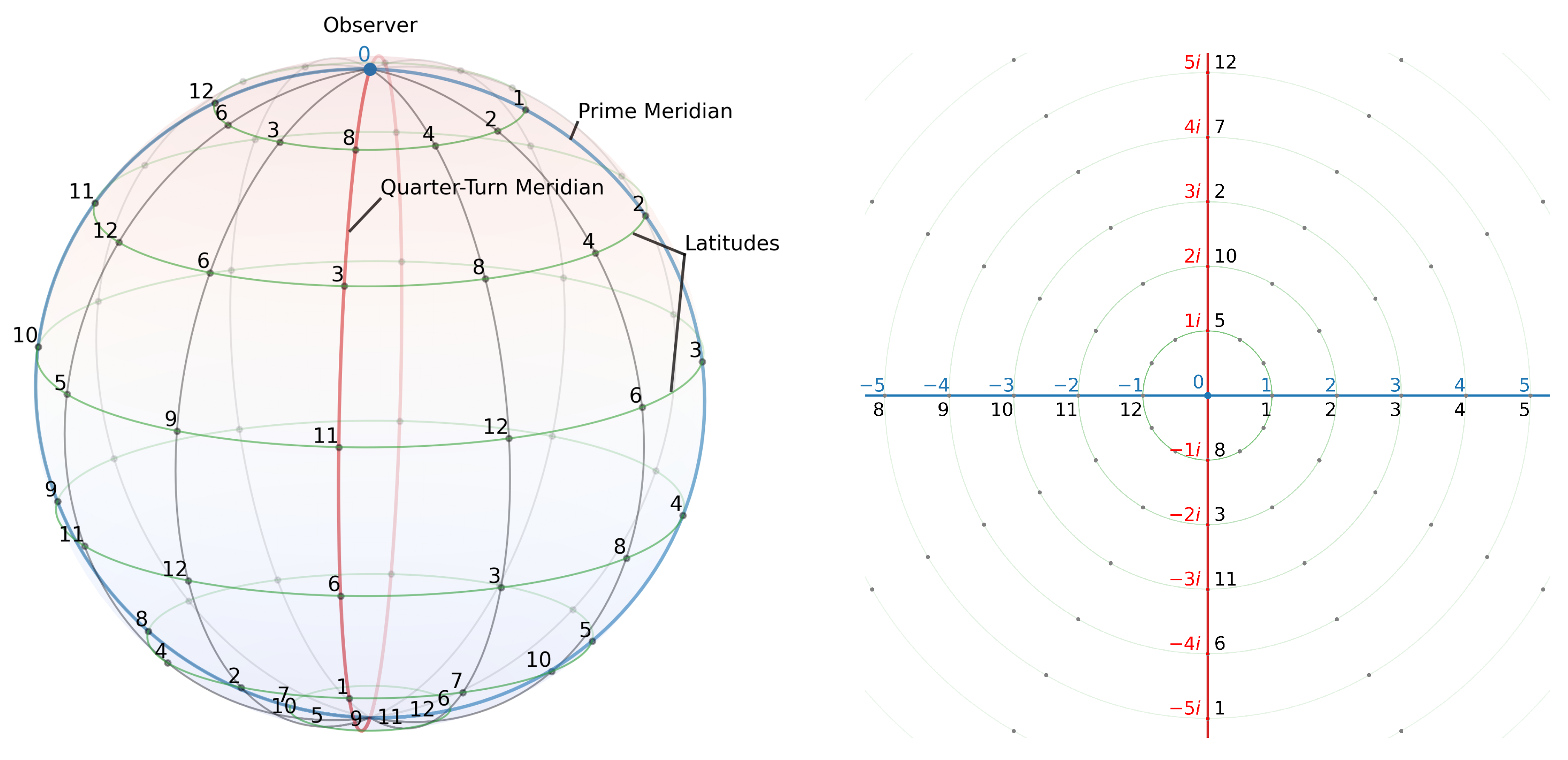
(Frame convention relative to the programme). The companion papers parameterize the extended frame by the exponential unit directly: there the frame datum is with the exponential unit itself the primitive generator and the quarter-turn induced from it, [33,38]. This paper takes the generator–turn pair as primitive — the turn is the Fourier datum of the spectral reading — and derives the exponential unit . The present datum thus adds an independent orientation choice for the quarter-turn, and the oriented need not be the induced one: in Figure 1 it is . Statements cited from the companion papers are convention-independent; only the labels , , must be converted between the two parameterizations.
Read together, the two actions cellulate the shell into a combinatorial 2-sphere [32]: the additive action generates the meridians, the multiplicative action the latitudes. A vertex carries an additive coordinate and a multiplicative phase ,
the origin common to every meridian: fixing m and varying a traces a meridian, while fixing and advancing m — multiplication by — traces a latitude. There are meridians (great circles) and latitudes, each set closed under the parity involution — equivalently the half-period phase shift — which pairs it into involution-partners. The distinguished additive line is the prime meridian, the spatial chart along which the prime-counting vector is read (Section 3); its Fourier dual, the quarter-turn meridian [38], is the spectral chart on which the zeros live (Section 4). Figure 1 shows both charts for , : the generator is , the oriented quarter-turn , the exponential unit , and the half-period .
Figure 1.
The framed shell with primitive generator , oriented quarter-turn , exponential unit , and half-period . Left: the orbital 2-sphere — the observer origin 0 at the north pole, the additive prime meridian (blue), the quarter-turn meridian (red), and the multiplicative latitudes (green). Right: the framed-complex Euclidean chart over — the prime meridian as the real axis, the quarter-turn meridian as the imaginary axis (), and the latitudes as norm circles [32].
Figure 1.
The framed shell with primitive generator , oriented quarter-turn , exponential unit , and half-period . Left: the orbital 2-sphere — the observer origin 0 at the north pole, the additive prime meridian (blue), the quarter-turn meridian (red), and the multiplicative latitudes (green). Right: the framed-complex Euclidean chart over — the prime meridian as the real axis, the quarter-turn meridian as the imaginary axis (), and the latitudes as norm circles [32].
Definition 1.2
(Carrier and Subject: the two complementary frames). The construction uses two nested symmetry-complete shells.
The Carrier is the field with prime — the arithmetic substrate, the totality — framed on its primitive generator , with origin 0 and space quantum (the Planck length), whose quarter-turn dual is the action quantum . Its exponential unit is a high-index power of that only appears transcendental when the shell is read through the degenerate continuum idealisation.
The Subject (the observer) is the field with prime, framed on its primitive generator , with origin 0, unit 1, and exponential unit . It is a local shell nested far inside the Carrier: , so the coherence horizon clears the Subject’s full range. Below the Subject horizon the two frames agree on arithmetic and primality, so finite statements there are frame-independent (Section 2).
Time in the framework is scale-dilation [34], which is why the dilation generator governs the spectral side.
1.3. The Epistemological Setting
On the shell the zeros are not scarce. Theorem 4.1 shows the finite zeta vanishes on every nonterminal exponent: the zeros are the whole nonterminal spectrum of the Carrier — all of but terminal unit , filling every geodesic slot, and under framed rational refinement they are dense in every finite interval of every geodesic. The classical question, is the real part of a zero equal to ?, therefore has no content here. It presupposes a scarce, individuated zero with a free real coordinate; the shell has no such scarce zero and no such free real coordinate. Every realised mode carries the one real part the construction admits, the half-turn (Proposition 5.4). Locating a zero on the line is vacuous, true of every mode by construction.
What is not vacuous is reconstruction. The prime-counting vector over the prime-meridian residues is one occupation of this universal basis, and rebuilding it is the problem of taking the modes in the right order. The flat direct-current mode carries nothing; the energy-bearing modes begin at the antipode and descend. In the units chart the per-mode energy is on squarefree q, maximal at the antipode — oddness — and falling thereafter, and the descending-energy sequence, antipode first, assembles the prime-counting staircase (Section 6). The Riemann Hypothesis, in these terms, is not where the modes sit but in what order they rebuild v — whether the on-line spectrum, taken in descending energy, reconstructs v with nothing left over (the units-chart energy order in which the staircase emerges and the zero-mode order in which completeness is stated are kept apart in Remark 7.5).
Why the modes carry the half-turn and no other real part is itself structural, and it is the same fact that makes the primes natural numbers. Primality is frame-relative: over the rationals or the complex plane it dissolves, and over the integers it survives only up to units. A prime is a resonance the Subject reads on the prime meridian, inside the window where the Subject and Carrier frames coincide (Proposition 2.1) — the real locus of agreement between observer and totality. The self-dual line is the one complex locus of that same coincidence. The real part is fixed there for the reason the primes are fixed on the naturals: both are where the two frames agree, and the construction reads only where they agree. This is the structural reason the modes are on the line — the agreement locus the reading is confined to — and equally the reason the reading is silent about anything off it.
The reconstruction of v from this window is not exact, and the inexactness is structural. The Subject shell does not close cleanly inside the Carrier: is a field, so is not an ideal of it, and the two grids — residues modulo p and modulo — coincide only below the horizon and diverge above it. The de-framing reads inside the agreement window, with a residual that is the contribution of the data beyond it, of order (Numerical Observation 7.3). At the physical Carrier ( in Planck units, the de Sitter entropy, coherence horizon ) the primality signal sits at the floor (Proposition 6.4, Numerical Observation 6.5) and is spread across the resolving frequencies up to the horizon (Numerical Observation 6.3), so the reconstruction washes out under every achievable resolution. In the Subject’s frame it is therefore quasi-stable: exact on the agreement loci, with a leak off them that shrinks as the shell grows but closes at no nested shell.
Whether the reconstruction closes exactly — zero leak — is the completeness question, and it turns on one arithmetic distinction: v is generated by a single multiplicative structure exactly when its series is an Euler product. The zeta function and the Dirichlet L-functions each carry one; a series without an Euler product carries none, its v a superposition of two structures whose interference lies on no single self-dual line, with off-line zeros to show for it. Section 10.4 makes this the Davenport–Heilbronn discriminator, the structural reason the rigidity of the real part is present for one Euler product and absent for a superposition. For a single Euler product the on-line spectrum is complete if and only if there is no off-line zero. And an off-line zero, were there one, is not a continuum artefact: it is a finite-height residue on a non-agreement meridian, frame-internal and in-field evaluable (SubSection 10.5) — exactly the type the framework retains. Completeness is therefore not discharged by declining the continuum, because the object that would break it is itself an FRC object, off the agreement loci, in the leak.
The hypothesis is : a single universal quantifier over heights — no zero lies off the line at any height. That quantifier is the whole of its difficulty. A false statement has a finite witness, an off-line zero at a computable height, and is refutable; a true one need not be provable, and cannot be confirmed instance by instance, for the instances are unboundedly many. The unbounded quantifier is the locus of the incompleteness to which such statements are exposed — truth outrunning proof.
The finite totality bounds it. With the Carrier finite (the reductio of [1]), heights range only to the coherence horizon , and the universal becomes no off-line zero at height — bounded, decidable in principle, carrying no incompleteness obstruction. The line then splits in three. Below the maximum conceivable observer horizon, height — the window of the largest admissible Subject, not any real observer’s — the question is verifiable, and is so far answered: no off-line zero, computed to height [39], still far below the horizon. From to the coherence horizon the zeros exist but lie past the observer’s resolution, where the reconstruction washes out at the floor — the quasi-stable band, the leak. Beyond the height chart wraps: the horizon is the no-wrap bound by definition, so a height symbol denotes, in-frame, its residue on the meridian cycle — a sub-horizon point relabelled, not new ground. The classical hypothesis quantifies over that third region as though it were populated with new heights; under the closed chart it is identified with the sub-horizon cycle, not populated. RH’s irreducible residue is therefore the bounded completeness clause below the horizon — relocated, not removed — and the unbounded quantifier that exposed the hypothesis to incompleteness is, once the totality is finite, closed by the topology of the chart rather than bounded by decree.
1.4. Outline of the Argument
The prime-counting function is a vector of amplitudes over the residues of the Subject field, read from the origin out to the horizon . Its spectral representation lives on the quarter-turn meridian of the finite fractional Fourier transform [38], where the nonterminal residues are the spectral modes — the finite zeta zeros. The flat mode at the spectral origin carries no prime information; the energy-bearing modes sit at the antipode, reached from the origin by the half-turn bias , so the spectral readout is the self-dual line , the finite critical line, and the zeros carry the form . The prime-counting staircase is the superposition of these modes, a Möbius-weighted resonance whose antinodes are the Subject-realized primes.
Two facts connect this finite picture to the classical theory. First, the de-framing functor from the shell to the analytic zeta is the finite Riemann–Siegel reconstruction: the Subject horizon is the Riemann–Siegel main-sum length, the half-turn is the critical-line weight, the scale coordinate is , and the Riemann–von Mangoldt zero density is exactly the multiplicative scale-depth of the shell. Second, the zeros are realised as the spectrum of the scale-evolution generator : the explicit formula is its trace formula, the prime-counting reconstruction is its trace, the realised modes are its eigenvalues, and self-adjointness at a finite shell makes its spectrum real. The reconstruction is read along the critical line and recovers the zero heights, so the placement of those eigenvalues on the line is structural. Classical RH is then the statement that the de-framing is faithful — that the on-line points it produces are the zeros themselves, not height-matched phantoms. This is the finite-shell form of the Hilbert–Pólya criterion (Section 8). The same construction applies to the -twisted prime-counting vector, a Dirichlet character on the units chart that leaves the self-dual structure untouched. It places the Dirichlet L-zeros on the line by the identical mechanism, so the generalized hypothesis reduces on the same footing.
Section 2 and Section 3 fix the two shells, the prime meridian, and the residue-vector. Section 4 places the spectrum on the quarter-turn meridian and identifies the modes with the finite zeta zeros. Section 5 locates the energy at the antipode and derives the critical line. Section 6 builds the prime-counting staircase from the modes. Section 7 constructs the de-framing functor. Section 8 exhibits the zeros as the scale-evolution spectrum, computed from the prime side, and states the reduction of the hypothesis; Section 10 develops the ontological promotion. All finite statements are exact algebra; the numerical observations are flagged as such, and the figures reproduce them.
2. The Carrier and Subject Shells and the Prime Meridian
2.1. Two Nested Shells
The FRC uses two prime fields, both with cardinality — the symmetry-complete condition that makes the multiplicative group divisible by four and admits a genuine quarter-turn. These are the Carrier () and the Subject () of Definition 1.2, nested so that the Carrier’s no-wrap horizon clears the Subject’s full range.
The two frames differ in their unit. The Subject’s unit is 1; the Carrier’s unit is the space quantum , the Subject’s sub-resolution length, whose quarter-turn dual is the action quantum . For the arithmetic of Section 3, Section 4, Section 5 and Section 6 the value of is invisible, because that arithmetic happens at the Subject scale where the two frames agree (SubSection 2.3); becomes critical only in Section 8, where it is the cutoff of the scale-evolution operator. Objects are finite sets read through the Subject frame; they play no role in the prime-counting construction and are omitted.
2.2. The Prime Meridian
The additive line of the Subject — the residues read as positions — is the prime meridian, the spatial chart of the shell [33]. A primitive coordinate becomes a natural number and a residue once the Subject frame is selected; before that it is an unframed mark on the field. The multiplicative structure equips the prime meridian with a second, cyclic coordinate: the discrete logarithm relative to a generator , the latitude, which records scale rather than position.
2.3. Coincidence Below the Horizon
The Subject’s no-wrap horizon is [34]. Below it, neither shell has wrapped, and the two frames agree on both arithmetic and primality.
Proposition 2.1
(Frame coincidence below ). For the residue n in and in is the same integer, and n is prime as a natural number if and only if it is irreducible in the Subject chart. Primality below is frame-invariant.
Proof.
Since , the integers are all smaller than , so no reduction has occurred in either field and the residues coincide. Primality of is decided by trial division by primes , all below the horizon, hence available and agreed upon within the Subject. Thus the Subject-realized primes
are exactly the primes below the horizon, shared by Carrier and Subject. □
This is the Russian-doll nesting of the FRC: the Subject’s full p residues encode prime content up to p, and the Carrier, whose coherence horizon lies far above p, certifies that content. The nesting is recursive — each shell’s horizon clears the next shell’s full range — and the Carrier, the totality, lies far above the local Subject.
3. The Prime-Counting Function as a Residue-Vector
The prime-counting function is usually treated as a map . In the FRC it is not a primitive of that kind. The shell carries a vector of amplitudes, one per residue, and the counting function is a particular reading of it.
Definition 3.1
(Prime-counting vector and its window). The prime-counting vector is the von Mangoldt amplitude
an amplitude assigned to each residue n. The windowed reading of v is its restriction to the no-wrap window: , read sequentially from the origin. The amplitudes at residues beyond the horizon are not read.
The classical prime-counting function is the cumulative windowed reading. To call v a “function” is to read it from the origin through the small values, ignoring what the amplitudes do beyond the horizon. This is the precise sense in which the horizon is a property of the reading, not of the object: the same vector v, read on a larger shell, exposes more of its prime content. Everything that follows is the spectral analysis of v and the recovery of its windowed reading.
4. The Spectral Representation: The Quarter-Turn Meridian
4.1. The Four Cardinal Meridians
The finite fractional Fourier transform over () is a rotation indexed additively along the meridian cycle , with four cardinal points at the quarter-turns [38]:
and . The half-period is , the parity point. The Fourier transform is the quarter-turn that carries the spatial prime meridian to the spectral meridian. On the spectral meridian each residue is a spectral mode of the vector being transformed.
4.2. The Modes Are the Finite Zeta Zeros
The available modes are the spectral content of any vector over , and they are governed by the orthogonality of the power character.
Theorem 4.1
(Zero-slot). For the finite zeta ,
The nontrivial spectral slots are exactly the nonterminal exponents: every one is a zero of .
Proof.
Let g generate . Then is a geometric sum. If each term is 1 and the sum is in . Otherwise and the sum is . This is character orthogonality. □
Thus, the finite zeta is degenerate as a value — it vanishes on every nontrivial slot — and what is informative is the family of zeros: the nonterminal residues, occupying every geodesic slot of the shell. They are the universal spectral basis, the energy levels available to any vector, observed on the spectral meridian because that is where modes live. The prime-counting vector v is one occupation of this basis. Two senses of zero therefore coexist and must be kept apart: the finite zeta zeros are the nonterminal slots, the universal mode basis; the classical zeros of are the particular modes that basis contributes to v, recovered by the de-framing (Section 8). The basis is the arena; the classical zeros are v’s occupation of it. The remaining question — in which order the modes are taken — is answered in Section 5.
The spectral and additive slot families are not merely equinumerous but structurally complementary, a fact that organizes the mode basis.
Theorem 4.2
(Slot complementarity). The nontrivial spectral slots and the nonterminal additive slots are each a single-point complement of ; the two removed points are the two elements of . The map is a bijection whose intertwiner is the half-cycle element of order two.
Proof.
removes the full-cycle exponent ( under ); removes . The map is the cyclic identification , and negation is multiplication by the order-two element ; composing gives the bijection , which carries the removed point of to the removed point of . □
5. Energy, the Antipode, and the Critical Line
5.1. Energy Needs the Quadratic Extension
To order the modes by energy one needs a genuine modulus, and the prime field carries none: has no nontrivial involution. Energy lives one extension up.
Lemma 5.1
(Hermitian phase calculus). Over with Frobenius involution , the norm and trace are -valued, phases lie on the unit circle of order on which Frobenius acts as inversion, and energy is a genuine quadratic form. For the quarter-turn is Frobenius-fixed, hence real in and off the phase circle. The Frobenius-odd directions are instead the trace-zero elements: fix with , equivalently a nonsquare in ; then is an -basis with and . The base-field quarter-turn is not such an η, since is a square.
Proof.
admits only the trivial automorphism, so a nondegenerate Hermitian form requires the quadratic extension; supplies it. The norm-one elements form the kernel of , cyclic of order , and Frobenius restricted to is . For , is a square in , so is fixed by Frobenius and satisfies , placing it off the circle. A Frobenius-odd z () has , so ; with this forces a nonsquare, and for such an , , . □
5.2. The Spectral Origin Is Flat
The full units-chart sum is the constant reflection of the zero-slot.
Proposition 5.2
(Flat ground state). Let be the Ramanujan sum, the units-chart standing wave of period q. The full-modulus chart sum is constant: for all , the additive reflection of the zero-slot. The mode at the spectral origin carries no prime information.
Proof.
for every such n, since the complete character sum over is 0 and the term is 1. The constant mode is the direct-current component; it equals the mean and distinguishes no residue. □
5.3. The Energy Is at the Antipode
Reading the prime-counting vector in the spectral meridian, the structural energy is not spread but concentrated at the antipode of the spectral origin.
Numerical Observation 5.3
(Antipode dominance). The spectral energy of the prime-counting vector is globally maximized at the antipode (Nyquist) frequency , the period-two mode that detects oddness. In the units-chart basis the per-mode energy is on squarefree q, with a unique global maximum at the antipode and falling thereafter across the totient levels ; the prime modes read
and the additive-transform band energy peaks at the same antipode ( at ). The direct-current mode is flat; oddness is the single strongest signature of the primes.
5.4. The Half-Turn and the Critical Line
The antipode is a half-turn from the spectral origin, and the half-turn is the FRC bias.
Proposition 5.4
(Finite critical line). The half-turn bias is the residue . The spectral readouts (, with η the trace-zero generator of Lemma 5.1) satisfy the exact self-dual condition
so the finite critical line
has exactly p points. On it the energy is . De-framing divides the bias residue by the shell cardinality: the normalized real part is , so the exact trace-one line is read as the classical critical line , recovered in the de-framing limit.
Proof.
The multiplicative inverse of 2 in is , the half-turn up to the unit; in the meridian cycle one has , the self-inverse half-turn. For with the trace-zero generator of Lemma 5.1 (, a nonsquare), Frobenius gives , so and . The trace-one affine line is a coset of the trace-zero hyperplane , of size p. □
Three coincident facts fix , and their coincidence is why it is robust.
- (i)
- It is the antipode of the flat direct-current mode — the half-turn from the useless origin.
- (ii)
- It is the Nyquist/oddness mode — the global maximum of the prime-counting energy (Numerical Observation 5.3).
- (iii)
- It is the self-dual, parity-symmetric locus , forced by the reality of the prime-counting vector through the conjugate symmetry of its spectrum.
The transverse coordinate indexes the energy level, giving the form ; the finite energy carries the classical form under the de-framing , the nonsquare absorbed into the scale of the height coordinate.
6. Emergence of the Prime-Counting Staircase
6.1. The Units-Chart Resonance
Reading the prime-counting vector through the comparison layer of the Subject, the prime weights emerge as a Möbius-weighted superposition of units-chart modes.
Definition 6.1
(Resonance). The units-chart resonance at bandwidth L is , and the renormalized resonance is .
Theorem 6.2
(Resonance and the von Mangoldt weight).
- (a)
- (Units-chart form.) [40], supported exactly on the prime powers with weight .
- (b)
- (Convolution-inverse form.) , the Dirichlet–Möbius inverse of the logarithm, exact on the divisor lattice, with .
- (c)
- (Intertwiner.) , so the renormalized resonance .
The support is the prime powers in every form; the weight is for the units-chart resonance and the exact after the radical rescaling.
Proof. (a) is Hardy’s Ramanujan-sum expansion of . For (b), is the elementary ; Möbius inversion gives , and for drops the logarithmic term, leaving [41]. Part (c) divides (b) by (a). □
6.2. The Staircase from the Modes
Cumulating the renormalized resonance reconstructs the Chebyshev staircase from the spectral modes, added in energy order (antipode first). With one has , the prime-counting function emerging as bandwidth grows. Figure 2 places this beside the classical reconstruction of from Riemann zeros: the two columns reach the same staircase through two spectral decompositions of the same prime content — zeros are the oscillation frequencies of , units-chart modes are its divisibility structure.
Numerical Observation 6.3
(Horizon-scale resolution). There is a threshold such that for the prime powers in are exactly the positions where exceeds every non-prime-power value, and numerically up to slowly growing factors, placing the resolving band at the Subject horizon, strictly between the window scale H and the field scale . The resolving frequencies are the squarefree integers , generated multiplicatively by the Subject irreducibles (Figure 3, right).
6.3. Square-Root Cancellation and Primality Resolution
The resolving band sits at the horizon because no single mode does better. This is a finite statement about how sharply one multiplicative-chart mode detects primality, standing on its own, independent of any zeta correspondence.
Proposition 6.4
(Mean-square flatness). Let be the indicator of on the latitude and the multiplicative-chart modes. By Parseval the mean energy per nonconstant mode is , so the root-mean-square correlation of with a chart mode is exactly of order .
Numerical Observation 6.5
(Square-root cancellation). The maximal chart-mode correlation, not only the root-mean-square, sits at the floor: no single multiplicative character resolves primality, and the resolving information is spread across the full band of squarefree frequencies up to the horizon. This upgrades the Parseval mean of Proposition 6.4 from an statement to an one. Numerically the maximum is against the floor at , and against over the chart modes of a Carrier (Figure 3, left).
The route from the proved mean to the observed maximum is a collision-robust large sieve: a bound on the orthogonality constant of the chart modes under a constraint on collision count rather than full phase separation. The single functional to be controlled is the maximal chart-mode correlation , and the target is the flatness up to slowly growing factors: the maximum brought down to the root-mean-square floor of Proposition 6.4 and Numerical Observation 6.5. This is a self-contained problem in finite harmonic analysis on the shell, independent of the de-framing reconstruction — and of GRH-strength difficulty, not a lighter surrogate: is a maximal character sum over the primes up to , and the target is exactly the square-root cancellation that the generalized hypothesis itself delivers for such sums ( under GRH); self-contained does not mean easier.
7. The De-Framing Functor: Finite Riemann–Siegel Reconstruction
The functor carrying the framed finite picture to the classical analytic zeta is the finite Riemann–Siegel reconstruction, and its dictionary is forced.
Definition 7.1
(De-framing dictionary). The de-framing functor sends the shell to the Riemann zeta on the critical line up to height , under the identifications
The classical Riemann–Siegel main sum [4] is then the windowed reading of the prime meridian: the same weight is the half-turn that places the modes on . The dictionary itself is definitional; its consequences (Proposition 7.2, Numerical Observation 7.3) are where it is tested.
The functor reconstructs the zeros from finite-horizon data: the bare horizon-length sum already locates , with the single term setting the smooth count through the phase and the further horizon terms sharpening it. Two structural consequences follow.
Proposition 7.2
(Zero density is shell scale-depth: dictionary consequence). Under , the smooth (average) Riemann–von Mangoldt zero density equals the multiplicative scale-depth of the shell:
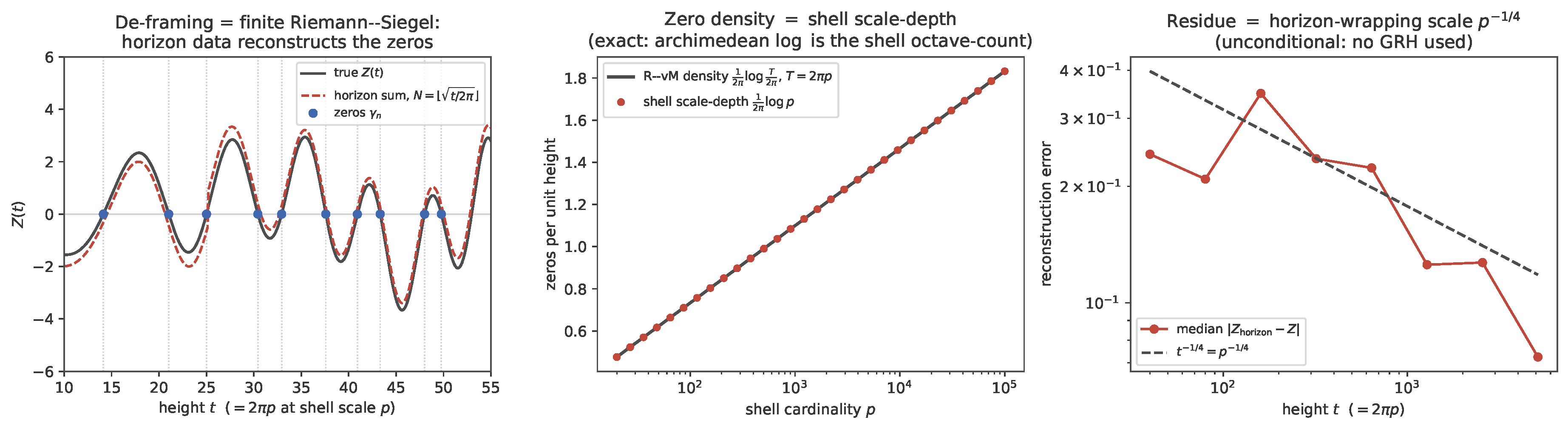
Equivalently : the smooth zero count to height is the shell’s scale-octave count. The smooth positions arise from the scale phase ; the fluctuations arise from the prime meridian. This is a substitution into the Riemann–von Mangoldt formula under the dictionary entry — a consistency of the dictionary, recorded as such, not an independent test of it.
Proof.
Numerical Observation 7.3
(Reconstruction residue). The finite-horizon reconstruction error is and is unconditional — pure truncation of the Riemann–Siegel main sum, requiring no hypothesis. The residue is the horizon-wrapping scale (Figure 4, right).
Figure 4.
The de-framing functor as finite Riemann–Siegel reconstruction. Left: the horizon-length sum (length , weight half-turn) tracks through the zeros. Center: the smooth zero density equals the shell scale-depth . Right: the reconstruction error follows , the horizon scale, with no hypothesis used.
Figure 4.
The de-framing functor as finite Riemann–Siegel reconstruction. Left: the horizon-length sum (length , weight half-turn) tracks through the zeros. Center: the smooth zero density equals the shell scale-depth . Right: the reconstruction error follows , the horizon scale, with no hypothesis used.
Lemma 7.4
(Completeness criterion). The following are equivalent:
- (a)
- the de-framing is faithful — the points it produces are the zeros of ζ themselves;
- (b)
- the on-line spectrum is complete for the prime vector v — the on-line mode expansion of the explicit formula rebuilds the windowed reading of v with no residual;
- (c)
- ζ has no off-line zero;
- (d)
- the Riemann Hypothesis.
Proof. (c)⇔(d) is the definition. The reconstructed is real (Proposition 5.4), so the de-framing places every point it produces on , at the heights it recovers from the horizon-length sum. For (a)⇔(c): if every zero of lies on the line, the produced on-line points are those zeros (faithful); an off-line zero, recovered at its height yet placed on the line, yields a produced point that is not the actual zero — a phantom (unfaithful). For (a)⇔(b): faithfulness is exactly that the on-line modes account for every height present in v; an off-line zero is a contribution to v that no on-line residue supplies (incompleteness of the on-line spectrum), and conversely a complete on-line spectrum leaves no height uncarried, hence no phantom. The incompleteness in (b) is moreover quantitative, not merely abstract: an off-line zero with (the functional equation pairs with ) contributes the term to the explicit formula, of amplitude against the of every on-line mode, so the residual of the on-line reconstruction grows as
a trace-detectable deficit at the phantom’s height, unmatchable by any on-line superposition of bounded relative amplitude. □
Remark 7.5
(Two spectral decompositions, one completeness clause). The paper carries two decompositions of the same prime content: the units-chart resonance of Section 6, with per-mode energy and the antipode first, and the zero-mode expansion of the explicit formula, with per-mode amplitude descending in height — the two columns of Figure 2. The completeness clause of Lemma 7.4(b) — and every subsequent statement that the on-line spectrum is complete for v — is stated in the zero-mode basis, where an off-line zero is a missing mode with the quantitative deficit exhibited in the proof. The units-chart order is where the staircase emerges (Theorem 6.2); the lemma asserts no transfer of completeness between the two bases, and none is used.
Corollary 7.6
(The reconstruction is on-line). The reconstructed is real, so every point it produces lies on (Proposition 5.4), recovered at the zero heights from the horizon-length sum. The on-line placement is thus structural — a property of how the reconstruction is read, along — so by Lemma 7.4 the classical Riemann Hypothesis is the completeness of this on-line spectrum for the prime vector, equivalently the faithfulness of the de-framing. The χ-twisted reconstruction is real by the same conjugate symmetry, so the corresponding statement holds for each Dirichlet L-function. The ontological reading, under which the de-framing produces the zeros as residues of the Carrier and the placement becomes a construction identity, is developed in Section 10.3.
8. The Zeros as the Scale-Evolution Spectrum
The reconstruction of Section 6 is the trace of an operator; the zeros are its spectrum. The bridge is one identity: the explicit formula is the trace formula of the scale-evolution operator.
8.1. The Scale-Evolution Operator
In the FRC, time is scale-dilation [34]: the natural evolution is the scale-shift [38], the rotation of the latitude by its generator, with idealising to the unit phase . Its generator is the scale-evolution generator .
Proposition 8.1
(Scale-evolution generator). The generator of the unitary scale-evolution is
The symmetrizing constant is the half-turn bias of Proposition 5.4: it is exactly the constant that makes self-adjoint and the real part of the critical line. The eigenstates are the critical-line characters.
Proof.
. The scale-shift rotates the latitude — on the shell an exact permutation of , hence unitary on — with idealising to the unit phase ; in that idealisation is a one-parameter unitary group, whose generator is self-adjoint with real spectrum by Stone’s theorem. The exact finite statement is the unitarity of the shell rotation; the differential form of , and its continuous spectrum, belong to the idealisation, discretised by the cutoff of Remark 8.3 and realised discretely from the comb in Definition 8.9. The symmetrizing constant is the half-turn bias of Proposition 5.4, the one datum that fixes the modes on the self-dual line and is the symmetrizer of . □
Corollary 8.2
(De-framing of the spectrum). The Hilbert–Pólya map is the FRC de-framing read on the spectrum:
where removes the half-turn bias and undoes the quarter-turn. The framed zero ρ maps to the real energy γ, and self-adjoint (real spectrum) is equivalent to every zero lying on , i.e. the Riemann Hypothesis.
8.2. The Cutoff, the Density, and the Periodic Orbits
The bare dilation has continuous spectrum; the zeros are discrete. The discretizer is the Carrier space quantum .
Remark 8.3
(Cutoff and semiclassical density: a heuristic correspondence). With the Carrier space quantum of Definition 1.2 as the lower cutoff (), the phase-space area of gives the semiclassical eigenvalue count
the Riemann–von Mangoldt count and the shell scale-depth of Proposition 7.2: the cutoff area is in the units , dividing by the cell to count states [21], and the Gutzwiller fluctuation sum over orbits of period is the prime side of the explicit formula [4]. The smooth spectrum is the scale dilation; the spectral fluctuations are the prime periodic orbits, of period at the Subject prime ℓ — the prime meridian. The correspondence is semiclassical, not derived from frame data: the cell normalization is imposed as the standard phase-space cell rather than obtained from the shell constants, and a consistent unit story for it is an open item of the framework. What is recorded is the correspondence itself — with the Carrier quantum as cutoff, the Berry–Keating count is the Riemann–von Mangoldt count.
8.3. The Spectrum from the Prime Side
The operator’s spectrum need not be read off from the zeros; it is already carried by the primes. On the scale axis , the spectral transform of the von Mangoldt comb is the logarithmic derivative, and its resonances are the zeros.
Proposition 8.4
(Prime–zero duality on the scale axis). The scale-spectrum of the von Mangoldt amplitudes,
continues to a meromorphic function whose poles are the point (the prime-number-theorem mode), the nontrivial zeros ρ, and the trivial zeros . On the self-dual axis the prime comb resonates precisely at the nontrivial zero heights . Equivalently, the eigenfrequencies that the prime-driven state excites in the dilation basis of (Proposition 8.1) are the zeros.
Numerical Observation 8.5
(The zero heights from the primes, with never evaluated). Truncate the scale-spectrum to a shell and apply a Cesàro taper,
This uses only the prime powers and their logarithms; is never evaluated. At the first six peaks of are
against
a maximum error of , each peak roughly seven times the baseline. The peak width is , so the resolving power is the scale-depth of Proposition 7.2, and the peaks sharpen as the shell grows. The independent estimator — the Fourier transform of the prime-counting fluctuation in the scale coordinate , built from the same — has the same peaks (Figure 5).
Two readings of the same correspondence now meet. The de-framing functor of Section 7 runs from the zeros to the primes — the finite Riemann–Siegel reconstruction evaluates the critical-line phase and recovers the prime fluctuation. Proposition 8.4 and Numerical Observation 8.5 run the other way, from the primes to the zeros, and share no step with it: the von Mangoldt comb is transformed on the scale axis and its resonances are the zeros, with never evaluated. The two directions are the two sides of the explicit formula — on one side, on the other — here computed independently and shown to agree. Reading the spectrum from the primes is the diagonalization of itself: the Fourier transform in is the diagonalization of the dilation generator (Proposition 8.1), and what it exposes is which eigenmodes the prime-driven state occupies — the zeros. What this exhibits is the spectral density of , the trace side peaked at the eigenvalues; the same data resolves into a discrete point spectrum through the trace, as follows.
8.4. The Discrete Spectrum as an Explicit Matrix
The density of the previous subsection sharpens into individual heights once it is read through the spectral counting function, and those heights are the roots of an explicit companion matrix built from the comb. The eigenvalue count of splits into an identity orbit and the prime orbits — the explicit formula — and the prime orbits are the comb.
Numerical Observation 8.6
(The discrete eigenvalues from the comb). Let be the archimedean scale-phase (the identity orbit, computed from , not from ), and let the prime orbits be the tapered comb
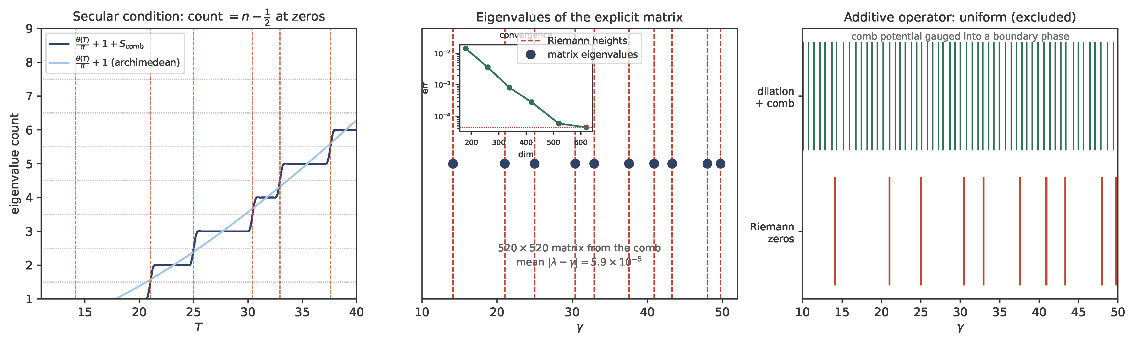
with w the raised-cosine (Cesàro) taper of Numerical Observation 8.5, required for convergence: the unweighted prime series for has partial sums that diverge as , and the raised-cosine window Cesàro-sums it, suppressing the truncation ringing and stabilising the secular crossings. The counting function crosses the half-integers at the zeros, as the tapered comb depth . Solving this secular condition for the eigenvalues, using only with never evaluated, numerically resolves the first ten heights to mean error at , sharpening with comb depth ( at , at ). The archimedean phase alone gives the mean positions (error ); the comb supplies the deviation of each eigenvalue (Figure 6, left).
Remark 8.7
(The limits are finitist refinements). The here, and in Numerical Observation 8.5, is not a completed continuum. Each step is a finite reframing to a finer scale along the meridian — the framed-rational refinement that carries the shell’s arbitrarily fine resolution from finite datum (SubSection 1.3). The comb depth N is the refinement depth and the resolving power is the scale-depth reached, so the limit is a horizon-relative degeneracy of the observer’s resolution, never a totality attained. The sharpening therefore invokes no completed infinity, consistently with the framework’s rejection of one.
Numerical Observation 8.8
(The zero heights from an explicit finite matrix). The secular condition is the characteristic equation of an explicit companion matrix. The secular determinant , built from the same archimedean phase and prime comb, vanishes at the zeros (in the comb limit). Expanded on a shell window in a Chebyshev basis, , its companion (colleague) matrix — whose entries are the comb-built coefficients — is a root-finder whose eigenvalues are the secular roots, hence the heights in the comb limit. Diagonalizing on returns the first ten heights to mean error at dimension 520, converging to the comb-truncation floor by dimension 620 as the dimension grows (Figure 6, center). The corresponding self-adjoint realisation is exhibited next, with the scattering form described in SubSection 10.5, and is never evaluated.
The colleague matrix is a root-finder, not symmetric; the self-adjoint operator it promises can be written down.
Definition 8.9
(Comb-built Jacobi realisation). Let be the secular roots of on a window (Numerical Observation 8.6) and the height measure they carry — both functionals of and the archimedean phase alone. The Jacobi realisation is the real-symmetric tridiagonal matrix of the three-term recurrence of the orthonormal polynomials of (Stieltjes–Lanczos): diagonal , off-diagonal . By the spectral theorem for finite Jacobi matrices its eigenvalues are exactly the atoms : is a manifestly self-adjoint operator whose spectrum is the comb-built heights.
Numerical Observation 8.10
(The Jacobi spectrum). On with the comb the ten recurrence coefficients are
and the eigenvalues of reproduce the secular roots to (machine precision) and the zero heights to mean error , the comb-truncation floor of Numerical Observation 8.6, with never evaluated. The matrix is explicit, real-symmetric, and tridiagonal: self-adjointness is exhibited, not asserted. The construction is deliberately elementary — any finite real multiset is the spectrum of such a matrix; what the exhibition certifies is that self-adjointness imposes no constraint, relocating the entire content of the hypothesis to faithfulness (SubSection 10.5).
The comb enters this matrix through the trace, not as a local potential: the additive form is excluded.
Proposition 8.11
(Additive injection is gauge-trivial). On , , the scale generator is , with uniform spectrum. For any real potential V, the operator is unitarily equivalent, by , to with a shifted boundary phase; its spectrum is uniform and depends on V only through . The comb therefore cannot produce the irregular zero spectrum by an additive potential: numerically, has spacing standard deviation of its mean against the zeros’ (Figure 6, right).
This gauge-triviality is the slot complementarity of Theorem 4.2 read dynamically. The nonterminal additive slots are the nontrivial spectral slots carried by the half-turn, , so an additive local potential is the gauge-trivial image of the spectral data — collapsing to a boundary phase — and the comb must enter multiplicatively, through the trace.
Figure 6.
The scale-evolution spectrum as a discrete spectrum, with never evaluated. Left: the counting function (archimedean phase plus the prime comb) steps through at the zeros (red). Center: the roots/eigenvalues of the explicit companion matrix of the comb-built secular determinant land on the heights (red), to mean error at dimension 520, converging to the comb floor ; inset, convergence as the dimension grows. Right: the additive operator has a uniform spectrum (Proposition 8.11), unlike the irregular zeros — the comb enters the trace, not a local potential.
Figure 6.
The scale-evolution spectrum as a discrete spectrum, with never evaluated. Left: the counting function (archimedean phase plus the prime comb) steps through at the zeros (red). Center: the roots/eigenvalues of the explicit companion matrix of the comb-built secular determinant land on the heights (red), to mean error at dimension 520, converging to the comb floor ; inset, convergence as the dimension grows. Right: the additive operator has a uniform spectrum (Proposition 8.11), unlike the irregular zeros — the comb enters the trace, not a local potential.
The scale-evolution spectrum is thus realized from the comb three ways, with never evaluated: as the spectral density (Numerical Observation 8.5), as the discrete eigenvalues of the secular condition (Numerical Observation 8.6), and as the roots/eigenvalues of the explicit companion matrix (Numerical Observation 8.8), with the self-adjoint realisation supplied by the comb-built Jacobi matrix (Definition 8.9, Numerical Observation 8.10). The two orbits — the archimedean scale-phase and the prime comb — are the two terms of the explicit formula, and their combination is the spectrum itself, the individual heights, not merely their density.
8.5. Random-Matrix Statistics
The discrete spectrum is not only correctly counted; its local statistics are those of a self-adjoint operator with chaotic classical dynamics.
Numerical Observation 8.12
(GUE level repulsion). The unfolded zero spacings exhibit level repulsion of the Gaussian unitary ensemble, not Poisson statistics: small spacings are suppressed as , with (GUE , Poisson ) and variance (GUE , Poisson 1) over the first 240 zeros [11,15]. In the FRC the GUE statistics are attributed to the mixing of the scale-evolution, with the discrete-logarithm scramble as the conjectured chaotic dynamics (Figure 7, left).
8.6. The Riemann Hypothesis as a Spectral Criterion
At every shell is a finite real-symmetric scale-evolution operator: its spectrum is real and lies on the self-dual line (Proposition 8.1). The de-framing (Corollary 8.2) reconstructs this structure along the critical line and recovers the zero heights. Reality of the spectrum is therefore structural — a property of how the construction is parametrized — and the content of the hypothesis is whether the de-framing is faithful: equivalently, whether the on-line spectrum is complete for the prime vector, in the zero-mode sense of Lemma 7.4 and Remark 7.5.
Theorem 8.13
(The FRC-realised zeros are the scale-evolution spectrum). The FRC-realised Riemann zeros are the finite-shell spectrum of . Under the de-framing (Corollary 8.2), this spectrum recovers the classical zero heights from the prime side. At each finite shell is self-adjoint, so its spectrum is real and lies on ; the half-turn is the self-adjointness symmetrizer and the critical real part at once. The Riemann Hypothesis is the faithfulness/completeness claim: equivalently, the claim that the on-line spectrum is complete for the prime vector v in the zero-mode sense of Lemma 7.4 (Remark 7.5), so that the on-line mode expansion rebuilds v with nothing left over for an off-line contribution. This is the finite-shell form of the Hilbert–Pólya criterion. Exact completeness is the zero-leak closure of the Subject reconstruction (SubSection 10.3), realisable in no nested Subject shell; the reductio [1] holds it out of scope rather than discharging it. The χ-twisted operator places the Dirichlet L-zeros by the identical mechanism, so the generalized hypothesis reduces on the same footing. The spectrum is exhibited from the prime side and resolved into individual heights (Proposition 8.4, Numerical Observations 8.5, 8.6 and 8.8). The scale-transform of the von Mangoldt comb resonates at the heights; the secular condition recovers the discrete heights to ; and the companion matrix of the comb-built secular determinant recovers those heights as its secular roots, the additive local form being excluded (Proposition 8.11). All of this holds with ζ never evaluated.
The faithfulness clause is not removable by the reconstruction itself. The counting function is the Riemann–von Mangoldt count of all strip zeros by height, and supplies on the line; an off-line zero would contribute to that count and surface as an on-line phantom at the same height. Such a zero is exactly an incompleteness of the on-line spectrum: a contribution to v that no on-line residue supplies, registering in the height count without an on-line mode to carry it. The construction, read on , recovers heights and is blind to the real part, so its eigenvalues are real whether or not the hypothesis holds. The numerical observations accordingly confirm the prime↔zero correspondence — the explicit formula computed from the prime side — and furnish an explicit prime-built matrix — the comb’s companion and self-adjoint Jacobi realisation — whose spectrum matches the zeros; they are consistent with the hypothesis and do not by themselves establish it. What they do establish unconditionally is structural, and is not a restatement of the hypothesis: the real part of the realised zero is the self-adjointness symmetrizer, fixed by the construction and carrying no free value, and the prime-side spectrum occupies that line. The hypothesis is thereby relocated — from a claim about the value of a free real coordinate to the completeness of the on-line spectrum for v, the faithfulness of the de-framing — and Section 10.4 shows this relocation is discriminating rather than vacuous, by exhibiting a Dirichlet series for which the same construction does not fix the real part.
Proposition 8.14
(The -twist and the generalized hypothesis). For a Dirichlet character χ, realised on the units chart through the multiplicative-chart modes of Proposition 6.4, the χ-twisted prime-counting vector carries the amplitudes of Definition 3.1 weighted by χ. For a real (quadratic) character the twisted vector is self-conjugate, the half-turn places the twisted modes on exactly as in the untwisted case (Proposition 5.4), and the construction goes through verbatim. For a complex character the functional equation pairs χ with rather than with itself, so reality of the twisted readout is not automatic: it requires rotation by the root number — with Gauss sum , conductor q, and parity — together with the twisted archimedean phase built from the matching Γ-factor of the completed . After this rotation the self-dual structure is restored, is self-adjoint with real spectrum, and the secular condition and companion matrix take the same form with the χ-twisted comb; the de-framing then carries the modes to the zeros of . Theorem 8.13 and its phantom therefore hold for each : unconditionally the generalized Riemann Hypothesis is the faithfulness of the twisted de-framing, on the same footing as the Riemann Hypothesis.
Numerical Observation 8.15
(Twisted-comb validation). For the real character (conductor 4, odd, root number 1), the twisted secular condition — the twisted archimedean phase and the -weighted comb, with no pole term — crosses the half-integers at the zeros of : evaluated at the first six zeros, located independently via Hurwitz zeta as the validation arm, it reads , , , , , . Solving the twisted secular condition with the comb, L never evaluated, recovers the six heights , , , , , to mean error — the comb-truncation floor of the untwisted case, substantiating the verbatim claim of Proposition 8.14.
Corollary 8.16
(The hypothesis reduces to the zero-leak closure). By Lemma 7.4 the Riemann Hypothesis is the completeness of the on-line spectrum for v, and exact completeness is the reconstruction at zero leak — the Subject and Carrier grids coinciding everywhere, realisable only in the Carrier’s frame and in no nested Subject shell (SubSection 10.3). The construction thus reduces the hypothesis, and through the χ-twist (Proposition 8.14) the generalized hypothesis, to that single object. With the Carrier finite (the reductio of [1]) the quantifier over heights is closed at the coherence horizon — the height chart wraps, so a putative trans-horizon zero aliases to a sub-horizon residue; this does not discharge completeness below the horizon, which would require excluding a finite-height, frame-internal residue the construction retains. That the reduction is structural and not a definition — the Davenport–Heilbronn case, in which the same construction does not fix the real part — is shown in Section 10.4.
9. Physical Interpretation
The substrate of the construction admits a physical reading: the Carrier is the Universe, the totality of admissible space-time coordinates; time is scale-dilation [34]; and the scale-evolution generator is its generator. On this reading the structure that realises the Riemann zeros and the structure of physics are one. The operator is physical time; the constants of physics are residues of the Carrier, built from the same quarter-turn and half-turn that order the zeros; and the half-turn that fixes the critical line is the square of the speed of light, . A finite reading of mass is outlook, fenced as such. None of this enters the realisation or the criterion: the Riemann Hypothesis result of the body stands independently of this section.
9.1. The Operator Is Physical Time
The operator is the generator of scale-dilation (Proposition 8.1), and scale-dilation is the flow of time in the framework [34]. It is fixed before any zero is invoked, so the realised zeros are the energy levels of physical time. On states the evolution is the time-dependent Schrödinger equation in FRC time, with stationary modes of energy — the zeros. The half-turn carries three roles at once — the self-adjointness symmetrizer of , the critical real part, and the self-dual rest locus (Propositions 5.4, 8.1) — one object, the antipode of the flat origin.
9.2. The Hard Core Is a Physical Law
The Carrier is finite, fixed at the de Sitter entropy in Planck units, with coherence horizon , the Hubble radius in Planck lengths. The primality signal correlates with no single mode above the floor (Proposition 6.4, Numerical Observation 6.5), the finest resolution the Universe affords. The energy-ordering that reconstructs the prime vector therefore lies beneath that floor and cannot be computed. In this reading the content of the hypothesis — whether that ordering closes — is a physical law about the substrate: the structural obstruction of SubSection 1.3 is also physical.
9.3. The Constants Are Residues of the Carrier
The additive prime meridian is space and the multiplicative latitude is time. The quarter-turn is the finite Fourier transform: it carries the prime meridian to the quarter-turn meridian, space to momentum [38]. On the same shell the classical constants are residues of the Carrier, transcendental only when read through the continuum idealisation: the exponential unit (SubSection 1.2), the circle constant , and the imaginary unit . A single residue, the half-turn, stands behind the finite Euler identities, read additively, as a quarter-turn squared, and multiplicatively,
with the critical real part .
The two quantum constants are the quarter-turn dressed by a scale. The action quantum is the quarter-turn dual of the Carrier’s space quantum (Definition 1.2),
and the speed of light is the quarter-turn carried over the shell curvature radius .
9.4. The Critical Line Is the Speed of Light
On a Carrier with the curvature radius is a residue, and the speed of light is the quarter-turn carried over it,
the quarter-turns cancel, leaving a real c: the axis-component of the unit lightlike direction along the cone that bisects the space-meridian and the time-latitude — the projection of the cone onto either axis, not its slope. Its square is the half-turn,
the critical real part on which the zeros lie (Proposition 5.4). The half-turn that places the zeros on the critical line and the square of the speed of light are one residue: the critical line is .
9.5. Outlook: A Finite Reading of Mass
The following will be developed in a companion paper and recorded here only to mark the direction. The quarter-turn is the shell’s Fourier transform: it carries the prime meridian to its spectral dual, position to momentum, as in the Weil representation [42]. That is de Broglie’s wave–particle duality. A mass is read on both charts: on the meridian as a localized rest configuration, with energy ; on the latitude, where time runs, as its Compton frequency, with . The two readings are one object.
Read this way, mass is cardinality: a mass m is a Subject of m degrees of freedom, and its rest energy is the share m of the totality’s , with the quarter-turn supplying the sign exactly as the de-framing carries to a real height. The corresponding Compton mode sits high in the spectrum of , near the cardinality scale, far above the low-lying zeros. A single identification fixes the scale: the locality horizon is the Planck mass. Sub-Planck masses are then deep inside the Subject horizon and local; the Planck mass is the boundary; a mass above it lies beyond the horizon, the regime where a local frame no longer closes; and the Subject whose mass is the whole Hubble mass has and is the Carrier itself. The known particle masses fall far inside the horizon, where they should. The relativistic completion is the Dirac equation on the quadratic-extension state space of Lemma 5.1,
with the explicit matrices over the extension satisfying the Clifford relations of the Lorentzian form whose temporal coefficient is the nonsquare , the exact finite differences, the Frobenius involution as the spinor conjugation, the quarter-turn as momentum, and the mass as the rest term; the first-order operator squares exactly to the finite Klein–Gordon operator — the finite Dirac layer [43]. The spatial multiplicity is left implicit: the framework derives the temporal–spatial split from the square class, not a count of spatial directions.
The spinor structure of that layer is already visible at the finite level, and it is the half-turn once more. On the quadratic extension of Lemma 5.1 the norm-one elements — the unit phase circle on which the body’s energy calculus runs, Frobenius acting as inversion — form the finite boost group of the Dirac layer [43], cyclic of order : in a finite frame the boosts close, and a complete turn of temporal evolution is a finite cycle. The norm- elements form the unique cyclic subgroup of order , and the squaring map carries it onto the boost group with kernel — the finite spin double cover. (The Hilbert 90 map , which carries the full onto with kernel , is not the cover here: on the norm- subgroup it equals with the sign the norm, its kernel acquires the base-field quarter-turns , and its image drops to index two in the boost group.) A generator w has , so one complete temporal turn returns the frame to itself yet multiplies the spinor by
and only the second turn closes. The residue the paper has met as the self-adjointness symmetrizer, the critical real part, the rest locus , and the square of the speed of light is here the spinor holonomy of one complete turn of time — the finite form of the sign a spinor acquires under a rotation, the factor two that separates the spinor period from the frame period , the structure Schrödinger read in the Dirac equation as the Zitterbewegung. The first-order factorization exists because temporal evolution acts through this double. The cycle itself is half-turn complete but quarter-turn incomplete: while , so temporal evolution owns the parity , with Frobenius as its time reversal, but hosts no internal quarter-turn — that must be borrowed from the spatial chart, which is the finite content of the Lorentzian . On the mass reading above, the Compton clock of a rest mass runs on this cycle, frame period against spinor period : the internal doubling of the relativistic electron, present in the shell as exact arithmetic.
The exact unit-quantum residue and the exact action-count of the totality are not pinned, and cannot be. They lie below , beyond the resolution of any finite observer. That they are unresolvable is the framework keeping faith with its own horizon, not a gap in it, the same status as an off-line zero at no finite height. What the reading offers is not these values but a finite, frame-relative account in which the constants, the mass–energy relation, and the critical line all descend from the one half-turn and the two horizons and .
10. Discussion
10.1. What Is Established
What follows spans three layers — exact finite algebra, classical analytic correspondence (the de-framing and zero density, Definition 7.1 and Proposition 7.2), and flagged numerical observation; only the finite-algebraic statements use no asymptotic or continuum input. The prime-counting function is a residue-vector read through the horizon (Definition 3.1). Its modes are the finite zeta zeros, the nonterminal residues on the quarter-turn meridian (Theorem 4.1). The spectral origin is flat (Proposition 5.2) and the energy is at the antipode (Numerical Observation 5.3). The half-turn bias places the spectrum on the self-dual line , read after de-framing as (Proposition 5.4). The prime-counting staircase emerges as the resonance , exact after radical rescaling (Theorem 6.2). The de-framing functor is the finite Riemann–Siegel reconstruction, with zero density equal to the shell scale-depth (Definition 7.1, Proposition 7.2). The realised zeros are the finite-shell spectrum of the scale-evolution generator , with the half-turn as its symmetrizer, the Carrier quantum as its cutoff, and GUE statistics (Section 8). That spectrum is exhibited from the prime side: the scale-transform of the von Mangoldt comb resonates at the zero heights, computed from with never evaluated, the reverse of the de-framing reconstruction. It resolves into the discrete heights both as the secular condition and as the roots of an explicit companion matrix built from the comb (Proposition 8.4, Numerical Observations 8.5, 8.6 and 8.8). These amount to a spectral realization and a criterion. The realised zeros are the on-line spectrum of a self-adjoint operator, its eigenvalues the zero heights, exhibited from the primes. Whether this spectrum is the zeros themselves, and not their height-matched image, is — since the reconstruction is read along the line — the completeness/faithfulness of the de-framing, the finite-shell Hilbert–Pólya criterion. The Riemann Hypothesis, with the generalized hypothesis through the -twist, is thereby equivalent to that criterion (Theorem 8.13, Corollary 7.6). The square-root cancellation of Proposition 6.4 and Numerical Observation 6.5 is a separate, self-standing result on primality resolution, not a residue of this criterion. The phrase “ never evaluated” is meant literally for the prime-side constructions: every prime-side computation uses only , their logarithms, and the archimedean phase from ; the de-framing of Section 7 reads the complementary, critical-line side. Known zero heights and zeta-side functions enter the figures solely as validation markers, never as inputs to any construction. That is never evaluated is a discipline of the spectral construction, not an inability of the framework: a convergent continuation of is available in-field — and, unlike the prime-side comb, would localise a zero’s real part directly — but that is the standard per-height verification (SubSection 10.5), not part of the realization. The construction earns the heights from alone, which is what separates it from a numerical evaluation of .
10.2. The Operator Picture
The operator picture is realised at each finite shell (SubSection 10.5). Section 8 identifies the scale-evolution operator , fixes its eigenvalue density as the shell scale-depth (Remark 8.3), and verifies its spacing statistics as those of the Gaussian unitary ensemble (Numerical Observation 8.12). Its spectrum is then produced from the prime comb at three levels of resolution, never evaluated. The first is the spectral density (Numerical Observation 8.5). The second is the discrete eigenvalues, as the secular condition of the archimedean scale-phase and the comb, to (Numerical Observation 8.6). The third is those same heights as the roots/eigenvalues of an explicit companion matrix, the comb-built root-finder whose entries carry the prime data (Numerical Observation 8.8). The comb enters this matrix through the trace, the additive local form being gauge-trivial (Proposition 8.11). The matrix exhibits the secular roots directly, and deeper shells sharpen the recovery, the floor being the comb truncation rather than the construction. The same companion construction, formed from the -twisted comb, carries the Dirichlet L-heights, in the manner of the trace formula of noncommutative geometry [22]. Two features separate this finite realisation from its continuum antecedents: the trace identity here is exact — finite character orthogonality (Theorem 4.1), not a regularised distribution — and the colleague matrix, a non-symmetric root-finder, has a genuine self-adjoint twin, the real-symmetric Jacobi matrix of the same height measure, its entries functionals of alone (SubSection 10.5).
10.3. The Finite Totality and the Reduction
Unconditionally, the body leaves the Riemann Hypothesis as a criterion (Theorem 8.13): the prime-side spectrum is real and lies on the self-dual line by construction, and what remains is the faithfulness of the de-framing — that the on-line points the reconstruction produces are the zeros and not height-matched phantoms.
The reductio of [1] is a formal reductio ad absurdum against completed infinity, argued independently of the zeta function and currently in peer review. Its conclusion is the one fact the reduction uses: the totality is finite. This places the construction in the finitist tradition in the foundations of mathematics and physics — the ultrafinitism of Yessenin-Volpin [44], the predicative arithmetic of Nelson [45], Zeilberger’s reading of real analysis as a degenerate case of discrete analysis [37], and, closest to the present setting, Lev’s reconstruction of mathematics and quantum theory on a finite ring, in which the classical continuum is a degenerate idealisation of the finite substrate [35,36].
This finitism is not, however, ultrafinitism. Ultrafinitism denies the existence of sufficiently large numbers, positing a largest feasible integer beyond which arithmetic ceases to apply [44]; the framework posits no such largest cardinality. The Carrier cardinality is not a maximal integer but a working cardinality, fixed by the coherence horizon . The cardinality scale is itself circular: the additive meridian and the multiplicative latitude both close on the shell, and the nesting is recursive, each shell’s horizon clearing the next shell’s full range (SubSection 2.3). So the scale has no terminal element and no maximum, only a horizon relative to an observer. What ultrafinitism would exclude as infeasible appears here instead as degeneracy. As a structure’s cardinality runs past the coherence horizon, its distinguishing complexity saturates: the primality signal sinks to the floor and is resolved by no single mode (Proposition 6.4, Numerical Observation 6.5). Its spectral domain degenerates too, the finite zeta vanishing on every nonterminal slot (Theorem 4.1). A very large structure is therefore not denied existence; it is only that a local finite observer cannot resolve it, and reads its spectrum as the degenerate value the shell reports. Finitude here is relational and horizon-bounded, not a ceiling on the integers.
Nor is the scale an ascending tower: it is closed. The meridian and latitude cycles close on the shell, and the recursive nesting runs inward — Subjects within the Carrier — so “no terminal element” names the closed topology of the scale, not a tower of actual cardinalities. One may count steps on a closed surface for as long as one has the energy to count; the count witnesses the non-termination of a traversal, not the infinitude of the substrate — the count is a process, the surface is a thing. Beyond the coherence horizon the height chart accordingly wraps: the horizon is the no-wrap bound by definition, so a height symbol denotes, in-frame, its residue on the meridian cycle, a sub-horizon point relabelled. The trans-horizon region is thereby identified rather than populated, and the bound on the quantifier is the closure of its domain — a property of the cyclic chart, not a denial of large magnitudes.
The derivation turns on a single structural fact established in the body: on the shell the real part of a zero is not an independent spectral datum. The half-turn is simultaneously the unique self-dual locus (Proposition 5.4), the self-adjointness symmetrizer of the scale-evolution generator (Proposition 8.1), and the critical real part; a residue of the Carrier read as a zero carries one free datum, its height , while its real placement is fixed by the representation domain. A zero off the self-dual line would require a real placement that the single-Carrier readout does not supply: the quadratic extension contains for every , but the reading is confined to the trace-one chart, where the real part, being the Frobenius trace, is pinned. Such a zero is realisable only by combining Carriers — a superposition of representation domains, no longer a single Euler product (the Davenport–Heilbronn witness, SubSection 10.4). One may add pears to a basket of apples, but the result is not a basket of apples. So the single-Carrier construction produces only on-line modes; this is the agreement-locus reading, and it pins the real part of the modes by construction. What it does not settle is whether those modes exhaust the zeros of — the completeness clause (Lemma 7.4), which the on-line reading is silent about because it reads only where the Subject and Carrier frames agree. On this footing the placement on is a construction identity at each shell, the unconditional content; the universal hypothesis is the exact completeness of the on-line spectrum, equal to the zero-leak closure — the Subject reconstruction with the two grids coinciding everywhere, realisable only in the Carrier’s frame and in no nested Subject shell (Theorem 8.13, Corollary 8.16). With the totality finite (the reductio of [1]) the universal quantifier over heights is bounded at the coherence horizon, emptying the trans-horizon residue; this does not discharge completeness below the horizon, which would require excluding a finite-height, frame-internal residue the construction retains.
The construction yields, unconditionally, the spectral realisation and the criterion. What the finite totality adds is the closure of the quantifier’s domain, and the consequence is priced openly: under the wrapped chart a putative trans-horizon off-line zero aliases to a sub-horizon off-line residue — exactly the finite-height, frame-internal object the corollary already retains — so the entire content of the trans-horizon region folds into the bounded completeness clause below the horizon. The bounding cleans the topology of the quantifier rather than deleting a populated region; it does no independent work beyond the concession already recorded. Two premises carry the closure, and both should be explicit: the finitude of the totality (the reductio of [1]) and the frame-covariance of the height chart — the identification of the classical height coordinate with the meridian cycle [32]. The wrap itself is shell algebra; only that identification is a framework premise. The disagreement between this reduction and a reader who declines it is therefore not about the zeta function, the spectrum, the implication, or the discriminator — it is about whether height symbols beyond the coherence horizon denote new ground or wrapped residues of old. That the criterion is discriminating rather than vacuous is the content of the next subsection.
10.4. The Euler-Product Discriminator
The reductio does not place all functional-equation zeros on the critical line, and it is essential that it does not. Consider the Davenport–Heilbronn function: a Dirichlet series that satisfies a Riemann-type functional equation but has no Euler product, formed as a fixed linear combination of two Dirichlet L-functions. It is a classical theorem that this function has infinitely many zeros off the critical line, including zeros in the half-plane of absolute convergence [3,31]. Any account on which RH followed by fiat — on which “every functional-equation zero lies on the line” were a definition — would be refuted by this function at once.
The framework is not refuted, because it predicts exactly this. The rigidity of the real part established in the body rests on a single symmetry-complete Carrier: one multiplicative group, one quarter-turn, one self-dual line . An Euler product is the arithmetic signature of such a single multiplicative structure — the zeta function and each Dirichlet L-function carry one. The Davenport–Heilbronn function carries none: it is a superposition of two multiplicative structures, and a superposition has no single self-dual line. Its zeros are not residues of one Carrier but interference nulls of two; an interference null is reachable by a finite combination of two shells — a finitely realisable object, free to sit off any single self-dual line, exactly as observed. In the language of Section 8 this is a manifest incompleteness: the on-line residue spectrum of a single Carrier is incomplete for the superposition that is the Davenport–Heilbronn vector, its deficit precisely the observed off-line zeros. For a single Euler product the corresponding completeness is exactly the hypothesis — the construction reads the same rigidity, but whether the on-line spectrum is complete is the zero-leak closure, not settled from inside the agreement window. The two cases are not symmetric: the superposition’s off-line zeros are finite interference nulls the construction reads directly; a single Euler product’s would be the failure of a completeness the construction cannot see. The discriminator is not left as an assertion; it is demonstrated, with a positive control.
Numerical Observation 10.1
(The discriminator demonstrated, with positive control). Take the Davenport–Heilbronn function , with the complex character mod 5 () and , computed via Hurwitz zeta functions; the completed is real on the line to , confirming the self-dual normalization. Counting strip zeros by the argument principle against on-line sign changes of , on : strip zeros against on the line — the phantom deficit , opening precisely in the band that holds the first off-line pair, located here at and its reflection [3]. On the line the rotated dips to at and does not cross: the strip holds two zeros there, the line holds none — the phantom is exactly the Turing-type inequality of SubSection 10.5, here exhibited live. The positive control: the identical pipeline on the constituent returns 45 strip zeros and 45 on-line zeros, deficit 0 in every band (Figure 8). One multiplicative structure, no phantom; a superposition of two, a phantom of two. The “ never evaluated” discipline does not bind this control arm, which validates the discriminator rather than the realisation.
This is the substance of the reduction, and the reason it is not a dissolution. It separates the case in which the real part is rigid (a single Euler product) from the case in which it is not (no Euler product), along precisely the line the classical theory draws between them, and it supplies the structural reason the classical theory leaves unexplained: the rigidity is the rigidity of a single self-dual line, present for one multiplicative structure and absent for a superposition. So the criterion is discriminating, not a definition — it places no functional-equation zero on the line by fiat, only the modes of a single Euler product, and only to the resolution the agreement window allows. What it does not deliver is the exact, universal completeness for : that is the zero-leak closure, held out of finite scope (SubSection 10.5). A reader who accepts the construction and the discriminator and still declines the universal statement is not disagreeing about the algebra, the prime-side spectrum, or the discriminator — only locating, correctly, the one object the framework does not reach: the closure in the Carrier’s frame, where the Subject and Carrier grids coincide everywhere.
10.5. What Is Settled, and What Is Not
The result is then three claims of decreasing strength.
The reduction. The placement on is a construction identity at each shell, and by Lemma 7.4 the universal hypothesis is the completeness of the on-line spectrum for v. Exact completeness is the zero-leak closure — the Subject reconstruction with the Subject and Carrier grids coinciding everywhere, realisable only in the Carrier’s frame and in no nested Subject shell (Theorem 8.13, Corollary 8.16). The construction reduces the hypothesis, and through the -twist the generalized hypothesis, to that single object; the finite totality bounds the hypothesis at the horizon, holding the trans-horizon residue out of scope (SubSection 10.3). That the reduction is structural and not a definition is fixed by the Davenport–Heilbronn case (SubSection 10.4).
Every finite height. At each finite height the hypothesis is decidable and, where checked, verified; the framework reproduces the verification frame-exactly and adds no certificate. The bounded clause below remains unverified beyond and, by the resolution floor of SubSection 9.2, uncomputable above in any Subject frame: decidable per height is not settled. The Riemann Hypothesis up to height N is the equality for all : the argument-principle count of strip zeros by height equals the number of on-line zeros, the sign changes of . This is Turing’s method [46], rigorous to height [39]. The framework supplies both sides of the equality with never evaluated. The comb gives , hence the total count ; the secular condition and its companion matrix exhibit the on-line heights (Numerical Observations 8.5, 8.6, 8.8). The shell carries no off-line mode — its nonterminal spectrum lies on the self-dual line (Theorem 4.1) — so an off-line zero of cannot be carried on-line and would surface as a phantom: a height the comb counts with no on-line mode to register it (SubSection 8.6), precisely the inequality that Turing’s count exposes. The construction reaches this window frame-exactly: by the dictionary of Definition 7.1 the de-framing realises to height with Riemann–Siegel length , and the comb amplitudes for coincide with their classical values (Proposition 2.1). To clear a window of heights it therefore suffices that the Subject horizon carry that window () and that the Carrier horizon clear the Subject (, no wraparound). At every finite height the framework thus matches the classical verification exactly and contributes consistency, not a new certificate; the analytic remainder (Numerical Observation 7.3) governs the numerical resolution of the reconstruction, not the existence of a counterexample. What no finite height settles is the height-free residue of the third claim.
The residue. What no finite shell reaches is the region beyond the coherence horizon — but under the closed chart that region is not a populated domain awaiting a verdict. The height chart wraps onto the sub-horizon cycle, so a putative trans-horizon off-line zero aliases to a finite-height, frame-internal residue, the very object the first claim already retains. Two premises carry this: the finitude of the totality ( degrees of freedom, the reductio of [1]) and the frame-covariance of the height chart [32]. The classical hypothesis is , a universal quantifier over heights; the closed chart closes the quantifier’s domain, and the hypothesis’s entire content is then the bounded completeness clause below the horizon. To keep a trans-horizon residue is to read the height symbols as new ground when the chart has already wrapped them. Below the horizon the question is the bounded, decidable-per-height one of the second claim; above it there is nothing new to decide.
The operator. The same finite-shell reading meets the standing objection that the dilation generator has continuous spectrum and so cannot be a Hilbert–Pólya operator. At each shell the operator is the discretisation of the bare dilation by the Carrier quantum (Remark 8.3), with discrete real spectrum; the continuous spectrum is its degenerate idealisation, as the continuum is the shell’s. The colleague matrix of Numerical Observation 8.8 is a root-finder and is not symmetric, so it is not itself the Hamiltonian; but its real spectrum carries a genuine self-adjoint realisation — the real-symmetric tridiagonal Jacobi matrix of the comb-built height measure, exhibited with its explicit entries in Definition 8.9 and Numerical Observation 8.10, the recurrence coefficients functionals of alone, whose eigenvalues are the heights exactly by the Stieltjes–Lanczos construction. Equivalently, on the scale interval bounded by the horizon, with the energy-dependent boundary phase , is a self-adjoint scattering problem whose quantisation is the secular condition — the finite analogue of , regularised by the no-wrap horizon the continuum lacks. A self-adjoint operator with the heights as spectrum therefore exists at every finite shell; that those heights are the zeros, and not merely their numerical image, is once more the completeness clause of the second claim. The operative moral deserves stating plainly: self-adjointness is free — any finite real multiset is the spectrum of a real-symmetric tridiagonal matrix, which is exactly what Definition 8.9 exhibits — and faithfulness is everything. The hard content of the Hilbert–Pólya programme was never the existence of a self-adjoint operator; it is whether the operator’s spectrum is the zeros rather than their image, and that is the completeness clause, with the phantom of Numerical Observation 10.1 as its operational signature.
10.6. Relation to the Programme and to the Classical Theory
The relational ontology and the frame-relative labels are the algebra of the programme [32]. The prime meridian, the quarter-turn meridian, and the finite fractional Fourier transform are its geometry [33], the transform realised as an exact meridian-cycle rotation, with the reversible scale-shift, in [38]. The quadratic extension, the Frobenius involution, and the finite Hermitian state space are its Euclidean–Lorentzian and Dirac layers [34,43]. Time as scale-dilation supplies the evolution whose generator is . The classical antecedents are exact: the explicit formula and the Riemann–Siegel reconstruction [4], the eigenvalue picture of Hilbert–Pólya and Berry–Keating [21], the trace formula of noncommutative geometry [22], and the pair correlation and spacing statistics of Montgomery and Odlyzko [11,15]. The contribution here is to realize them inside a finite, frame-relative framework in which the half-turn is a single object — the antipode, the critical real part, and the self-adjointness symmetrizer at once — and in which the zero density is the shell scale-depth.
11. Conclusion
One structure runs through the account. The prime-counting function is a vector over the residues of the Subject, read through the horizon . Its spectrum lives on the quarter-turn meridian; the flat direct-current mode carries nothing, and the energy sits at the antipode, a half-turn away. The half-turn is the bias , so the spectral readout is the self-dual line and the modes carry the form . The prime-counting staircase emerges from these modes as the units-chart resonance. The de-framing functor to the classical zeta is the finite Riemann–Siegel reconstruction, in which the horizon is the main-sum length, the half-turn is the weight, and the zero density is the multiplicative scale-depth of the shell. And the realised zeros are the finite-shell spectrum of the scale-evolution generator — the generator of FRC time — whose symmetrizer is the half-turn, whose cutoff is the Carrier quantum, whose orbits are the primes, and whose statistics are those of the Gaussian unitary ensemble. The half-turn is the self-adjointness symmetrizer of and the critical real part at once, so the finite spectrum is real by the same fact that places it on the line. The reconstruction is read along that line and recovers the zero heights. The Riemann Hypothesis — with the generalized hypothesis on the same footing through the -twist — is therefore equivalent to the faithfulness of the de-framing, the finite-shell Hilbert–Pólya criterion. The spectrum is moreover exhibited from the prime side: the von Mangoldt comb, transformed on the scale axis, resonates at the zero heights with never evaluated. This is the reverse of the reconstruction, and the spectral resolution of the finite scale problem. Read through the spectral counting function, it resolves into the individual heights, recovered from the comb to . That prime-orbit quantization is the characteristic equation of an explicit companion matrix built from the comb, with the additive local form being gauge-trivial and the self-adjoint realisation supplied by its Jacobi/scattering form. These constructions confirm the explicit formula from the prime side and furnish an explicit prime-built matrix — the comb’s companion/Jacobi realisation — whose spectrum matches the zero heights, consistent with the hypothesis. The placement on is a construction identity at each shell — the unconditional content — so the realised spectrum is on-line by construction; whether it is complete for v is the faithfulness of the de-framing (Corollary 8.16, Section 10.3). That the reduction is structural and not a definition is settled by a single test: the same construction, applied to a Dirichlet series without an Euler product, does not fix the real part, in accord with the off-line zeros of the Davenport–Heilbronn function (Section 10.4). The rigidity is the rigidity of a single self-dual line, present for one multiplicative structure and absent for a superposition. The realisation is unconditional; at each finite height the hypothesis is decidable and, where checked, verified, reproduced from the prime side with no off-line mode available (SubSection 10.5), and the in-shell reconstruction is quasi-stable — exact on the agreement loci, with a leak that closes at no nested shell. The hypothesis is , a universal quantifier over heights; the finite totality, with the frame-covariance of the height chart, closes that quantifier at the coherence horizon — the chart wraps, a trans-horizon symbol denoting a sub-horizon residue — leaving a bounded completeness clause below the horizon, relocated, not removed. The framework establishes that reduction and the quasi-stable verification; the residue it does not reach is the bounded clause itself, the closure in the Carrier’s frame, where the Subject and Carrier grids coincide everywhere.
Reproducibility
Every Numerical Observation of the realisation is computed from (sieved directly), the archimedean phase from , and standard linear algebra; no zeta-function library is invoked at any point, and the known zero heights enter only as validation markers in the figures. The two validation arms are the exception by design: the Davenport–Heilbronn control of Numerical Observation 10.1 and the reference L-zeros of Numerical Observation 8.15 evaluate Hurwitz zeta functions, since they validate the discriminator and the twist rather than the realisation. Complete scripts reproducing each observation and figure, together with the numeric validation suite, are available at https://github.com/gamayos/frc-rh.
References
- Akhtman, Y. Paradoxes of Infinity as Reductio ad Absurdum. Preprints 2025.
- Riemann, B. Über die Anzahl der Primzahlen unter einer gegebenen Größe. Monatsberichte der Königlich Preußischen Akademie der Wissenschaften zu Berlin 1859, pp. 671–680.
- Titchmarsh, E.C. The Theory of the Riemann Zeta-Function, 2nd ed.; Oxford University Press, 1986. Revised by D. R. Heath-Brown.
- Edwards, H.M. Riemann’s Zeta Function; Academic Press, 1974.
- Iwaniec, H.; Kowalski, E. Analytic Number Theory; Vol. 53, American Mathematical Society Colloquium Publications, American Mathematical Society: Providence, RI, 2004.
- Conrey, J.B. The Riemann hypothesis. Notices of the American Mathematical Society 2003, 50, 341–353.
- Bombieri, E. Problems of the Millennium: The Riemann Hypothesis. Clay Mathematics Institute, official problem description, 2000.
- Hardy, G.H. Sur les zéros de la fonction ζ(s) de Riemann. Comptes Rendus de l’Académie des Sciences Paris 1914, 158, 1012–1014.
- Levinson, N. More than one third of zeros of Riemann’s zeta-function are on σ=1/2. Advances in Mathematics 1974, 13, 383–436. [CrossRef]
- Conrey, J.B. More than two fifths of the zeros of the Riemann zeta function are on the critical line. Journal für die reine und angewandte Mathematik 1989, 399, 1–26. [CrossRef]
- Odlyzko, A.M. On the distribution of spacings between zeros of the zeta function. Mathematics of Computation 1987, 48, 273–308.
- Selberg, A. Harmonic analysis and discontinuous groups in weakly symmetric Riemannian spaces with applications to Dirichlet series. Journal of the Indian Mathematical Society (N.S.) 1956, 20, 47–87.
- Weil, A. Sur les “formules explicites” de la théorie des nombres premiers. In Communications du Séminaire Mathématique de l’Université de Lund (volume dédié à Marcel Riesz); Université de Lund, 1952; pp. 252–265.
- Siegel, C.L. Über Riemanns Nachlaß zur analytischen Zahlentheorie. Quellen und Studien zur Geschichte der Mathematik, Astronomie und Physik, Abteilung B: Studien 1932, 2, 45–80.
- Montgomery, H.L. The pair correlation of zeros of the zeta function. In Analytic Number Theory (Proc. Sympos. Pure Math., Vol. XXIV); Amer. Math. Soc., 1973; pp. 181–193.
- Mehta, M.L. Random Matrices, 3 ed.; Vol. 142, Pure and Applied Mathematics, Elsevier/Academic Press: Amsterdam, 2004.
- Rudnick, Z.; Sarnak, P. Zeros of principal L-functions and random matrix theory. Duke Mathematical Journal 1996, 81, 269–322. [CrossRef]
- Katz, N.M.; Sarnak, P. Zeroes of zeta functions and symmetry. Bulletin of the American Mathematical Society (N.S.) 1999, 36, 1–26. [CrossRef]
- Katz, N.M.; Sarnak, P. Random Matrices, Frobenius Eigenvalues, and Monodromy; Vol. 45, American Mathematical Society Colloquium Publications, American Mathematical Society: Providence, RI, 1999.
- Keating, J.P.; Snaith, N.C. Random matrix theory and ζ(1/2+it). Communications in Mathematical Physics 2000, 214, 57–89. [CrossRef]
- Berry, M.V.; Keating, J.P. The Riemann zeros and eigenvalue asymptotics. SIAM Review 1999, 41, 236–266.
- Connes, A. Trace formula in noncommutative geometry and the zeros of the Riemann zeta function. Selecta Mathematica 1999, 5, 29–106.
- Sierra, G.; Townsend, P.K. Landau levels and Riemann zeros. Physical Review Letters 2008, 101, 110201. [CrossRef]
- Bender, C.M.; Brody, D.C.; Müller, M.P. Hamiltonian for the zeros of the Riemann zeta function. Physical Review Letters 2017, 118, 130201. [CrossRef]
- de Branges, L. The Riemann hypothesis for Hilbert spaces of entire functions. Bulletin of the American Mathematical Society (N.S.) 1986, 15, 1–17.
- Lapidus, M.L. In Search of the Riemann Zeros: Strings, Fractal Membranes and Noncommutative Spacetimes; American Mathematical Society: Providence, RI, 2008.
- Schumayer, D.; Hutchinson, D.A.W. Colloquium: Physics of the Riemann hypothesis. Reviews of Modern Physics 2011, 83, 307–330. [CrossRef]
- Weil, A. Numbers of solutions of equations in finite fields. Bulletin of the American Mathematical Society 1949, 55, 497–508.
- Deligne, P. La conjecture de Weil. I. Publications Mathématiques de l’IHÉS 1974, 43, 273–307. [CrossRef]
- Rosen, M. Number Theory in Function Fields; Vol. 210, Graduate Texts in Mathematics, Springer-Verlag: New York, 2002.
- Davenport, H.; Heilbronn, H. On the zeros of certain Dirichlet series. Journal of the London Mathematical Society 1936, 11, 181–185.
- Akhtman, Y. Relativistic Algebra over Finite Ring Continuum. Axioms 2025, 14, 636. [CrossRef]
- Akhtman, Y. Geometry and Constants in Finite Ring Continuum. Symmetry 2026, 18, 751. [CrossRef]
- Akhtman, Y. Euclidean–Lorentzian Dichotomy and Algebraic Causality in Finite Ring Continuum. Entropy 2025, 27, 1098. [CrossRef]
- Lev, F.M. Finite Mathematics as the Foundation of Classical Mathematics and Quantum Theory: With Applications to Gravity and Particle Theory; Fundamental Theories of Physics, Springer: Cham, 2020. [CrossRef]
- Lev, F.M. Discussion of foundation of mathematics and quantum theory. Open Mathematics 2022, 20. [CrossRef]
- Zeilberger, D. “Real” Analysis Is a Degenerate Case of Discrete Analysis. In New Progress in Difference Equations (Proceedings of ICDEA 2001); Aulbach, B.; Elaydi, S.; Ladas, G., Eds.; Taylor & Francis: London, 2004.
- Akhtman, Y. Scale-Shift and Fractional Fourier Transform as Rotations in Representation Space over Finite Fields. Preprints 2026. [CrossRef]
- Platt, D.J.; Trudgian, T.S. The Riemann hypothesis is true up to 3·1012. Bulletin of the London Mathematical Society 2021, 53, 792–797. [CrossRef]
- Hardy, G.H. Note on Ramanujan’s trigonometrical function cq(n) and certain series of arithmetical functions. Proceedings of the Cambridge Philosophical Society 1921, 20, 263–271.
- Apostol, T.M. Introduction to Analytic Number Theory; Undergraduate Texts in Mathematics, Springer-Verlag: New York, 1976.
- Weil, A. Sur certains groupes d’opérateurs unitaires. Acta Mathematica 1964, 111, 143–211. [CrossRef]
- Akhtman, Y. Schrödinger–Dirac Formalism in Finite Ring Continuum. Preprints 2025. [CrossRef]
- Yessenin-Volpin, A.S. The ultra-intuitionistic criticism and the antitraditional program for foundations of mathematics. In Intuitionism and Proof Theory (Proc. Summer Conf., Buffalo, N.Y., 1968); Kino, A.; Myhill, J.; Vesley, R.E., Eds.; Studies in Logic and the Foundations of Mathematics, North-Holland: Amsterdam, 1970; pp. 3–45.
- Nelson, E. Predicative Arithmetic; Vol. 32, Mathematical Notes, Princeton University Press: Princeton, NJ, 1986.
- Turing, A.M. Some calculations of the Riemann zeta-function. Proceedings of the London Mathematical Society 1953, s3-3, 99–117. [CrossRef]
Figure 2.
Prime-counting function from spectral modes: classical zeros (left) and FRC units-chart modes (right). Top: the spectral modes — the lowest zeros and the units-chart modes in energy order (, the antipode/oddness, first). Bottom: the staircase emerging — from M zeros and from bandwidth L, both converging to the same . The FRC wiggle at low L is the analogue of the classical Gibbs overshoot at low M and tightens monotonically with bandwidth.
Figure 2.
Prime-counting function from spectral modes: classical zeros (left) and FRC units-chart modes (right). Top: the spectral modes — the lowest zeros and the units-chart modes in energy order (, the antipode/oddness, first). Bottom: the staircase emerging — from M zeros and from bandwidth L, both converging to the same . The FRC wiggle at low L is the analogue of the classical Gibbs overshoot at low M and tightens monotonically with bandwidth.
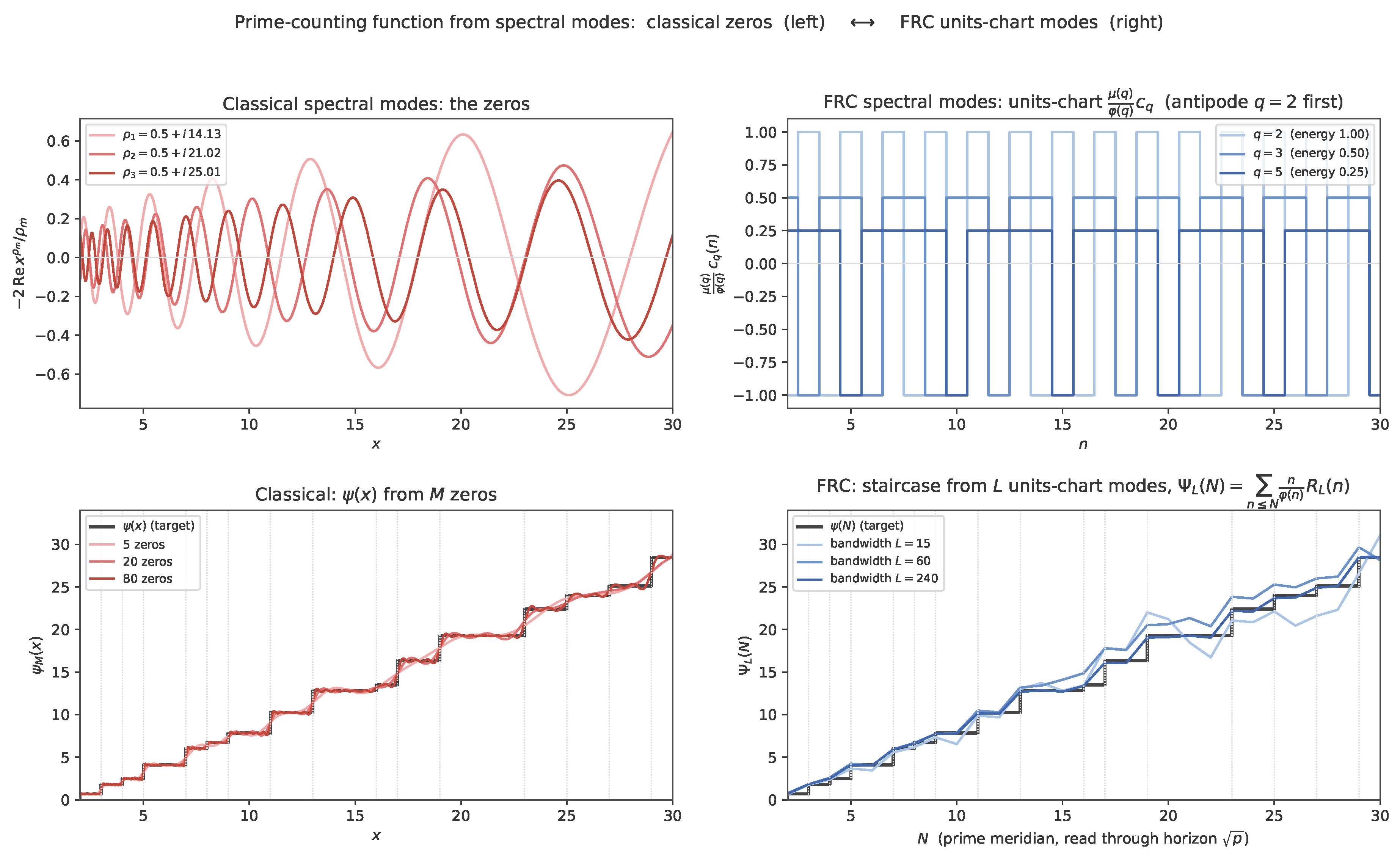
Figure 3.
The equidistribution obstruction and the resolving scale. Left: the correlation of the prime indicator with each multiplicative-chart mode at hugs the noise floor across all modes, while the units-chart resonance reaches (Numerical Observation 6.5). Right: the resolving threshold tracks the horizon and lies far below the field scale , reflecting prime-power thresholds (Numerical Observation 6.3).
Figure 3.
The equidistribution obstruction and the resolving scale. Left: the correlation of the prime indicator with each multiplicative-chart mode at hugs the noise floor across all modes, while the units-chart resonance reaches (Numerical Observation 6.5). Right: the resolving threshold tracks the horizon and lies far below the field scale , reflecting prime-power thresholds (Numerical Observation 6.3).
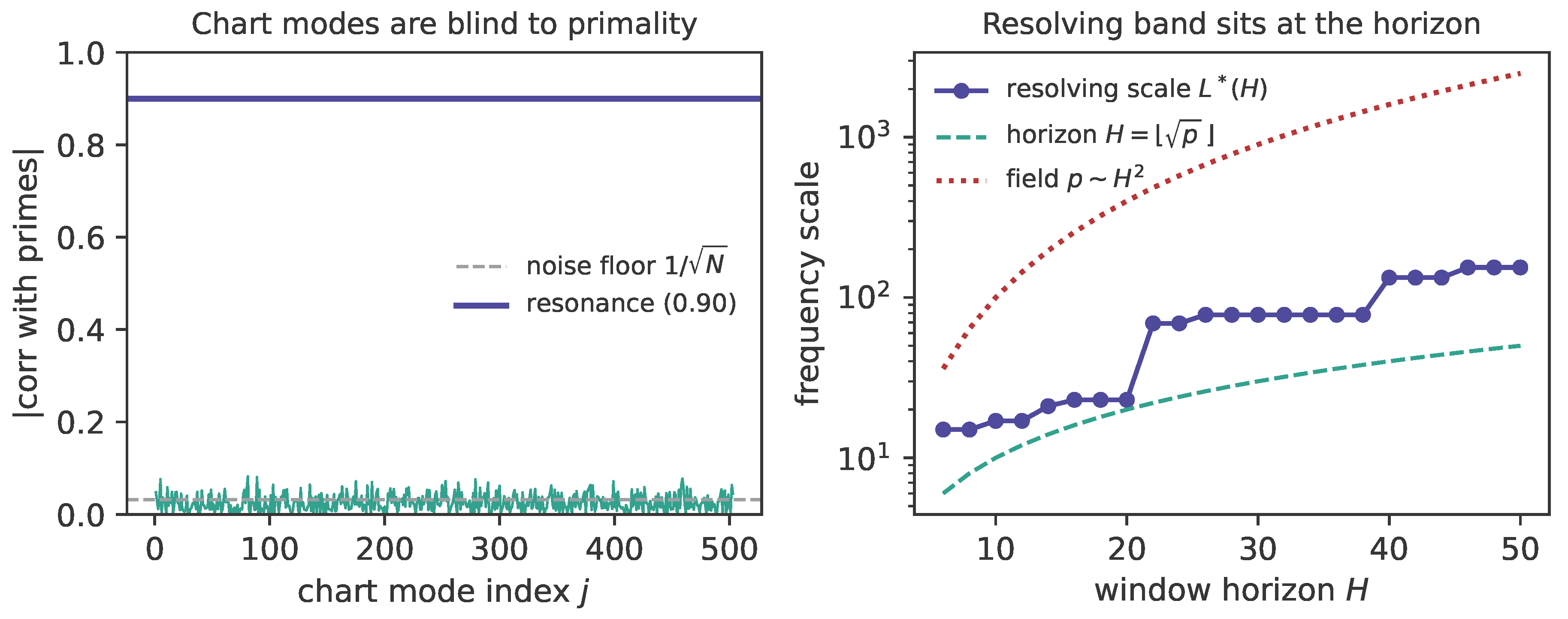
Figure 5.
The spectrum of read from the prime side, with never evaluated. Top: the scale-spectrum of the von Mangoldt comb at ; the peaks (orange) fall on the zero heights (red dashed). Middle: the independent estimator, the Fourier transform of the prime-counting fluctuation in the scale coordinate , with the same peaks. Bottom: the resolving power is the scale-depth — the peak at sharpens as the shell N grows, width .
Figure 5.
The spectrum of read from the prime side, with never evaluated. Top: the scale-spectrum of the von Mangoldt comb at ; the peaks (orange) fall on the zero heights (red dashed). Middle: the independent estimator, the Fourier transform of the prime-counting fluctuation in the scale coordinate , with the same peaks. Bottom: the resolving power is the scale-depth — the peak at sharpens as the shell N grows, width .
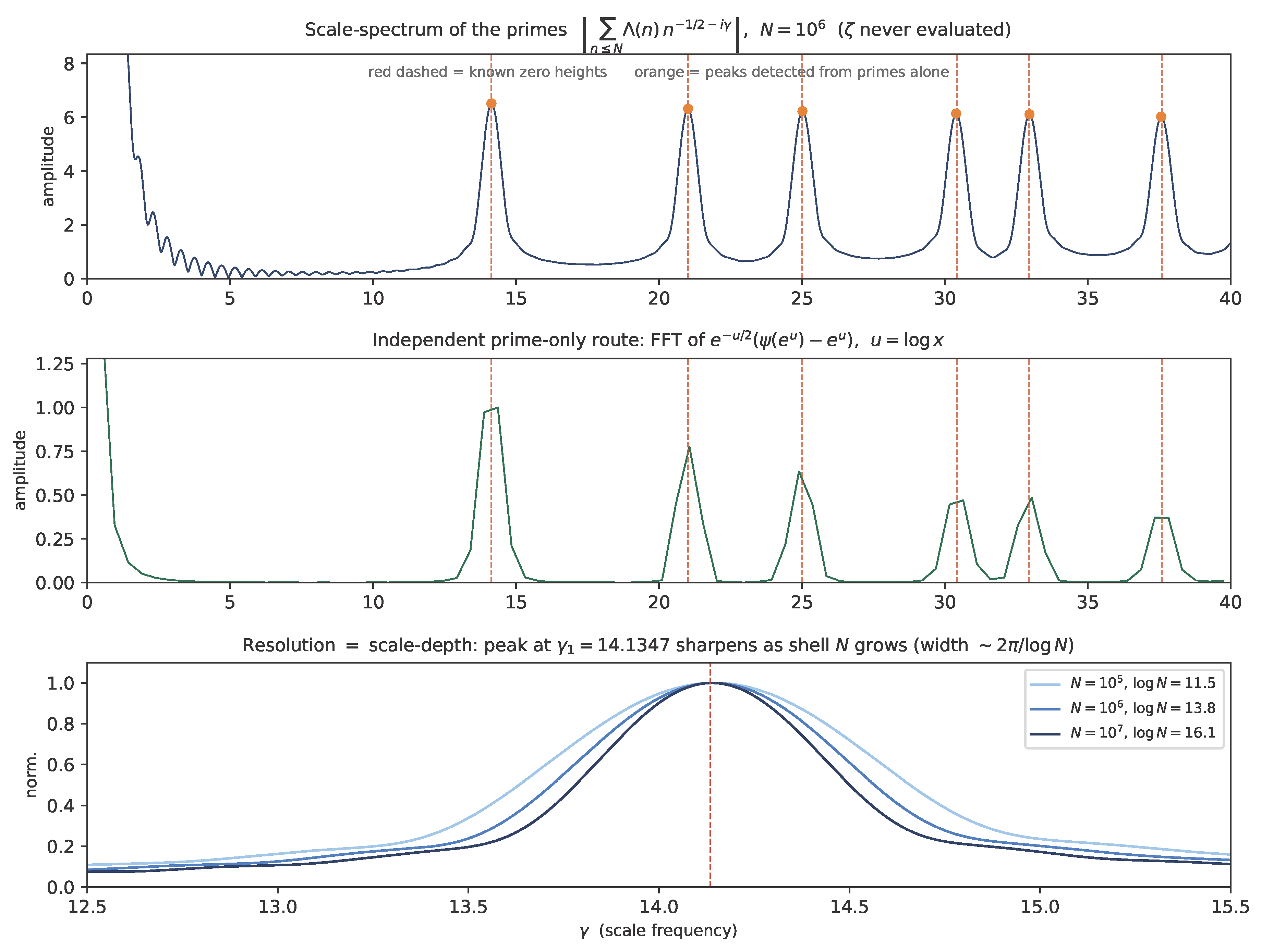
Figure 7.
The zeros as eigenvalues of the scale-evolution operator , with . Left: the unfolded spacings show GUE level repulsion, not Poisson — the spectrum of a self-adjoint operator with chaotic dynamics. Right: the eigenvalue count lies on the Berry–Keating semiclassical , i.e. density , the shell scale-depth with cutoff .
Figure 7.
The zeros as eigenvalues of the scale-evolution operator , with . Left: the unfolded spacings show GUE level repulsion, not Poisson — the spectrum of a self-adjoint operator with chaotic dynamics. Right: the eigenvalue count lies on the Berry–Keating semiclassical , i.e. density , the shell scale-depth with cutoff .
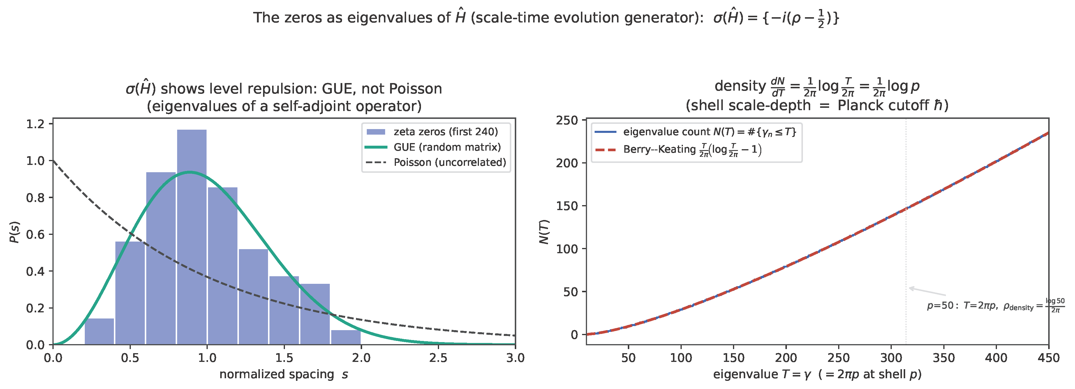
Figure 8.
The Euler-product discriminator demonstrated (Numerical Observation 10.1). Left: rotated on-line values on : the constituent crosses zero twice (two on-line zeros), while the Davenport–Heilbronn f dips at the off-line height without crossing — two strip zeros invisible to the line. Right: the cumulative strip count against the on-line count for f on : the staircases coincide until the off-line pair at , where the phantom deficit opens (inset: the gap; totals 45 against 43); the identical pipeline on the constituent closes with , deficit zero in every band.
Figure 8.
The Euler-product discriminator demonstrated (Numerical Observation 10.1). Left: rotated on-line values on : the constituent crosses zero twice (two on-line zeros), while the Davenport–Heilbronn f dips at the off-line height without crossing — two strip zeros invisible to the line. Right: the cumulative strip count against the on-line count for f on : the staircases coincide until the off-line pair at , where the phantom deficit opens (inset: the gap; totals 45 against 43); the identical pipeline on the constituent closes with , deficit zero in every band.
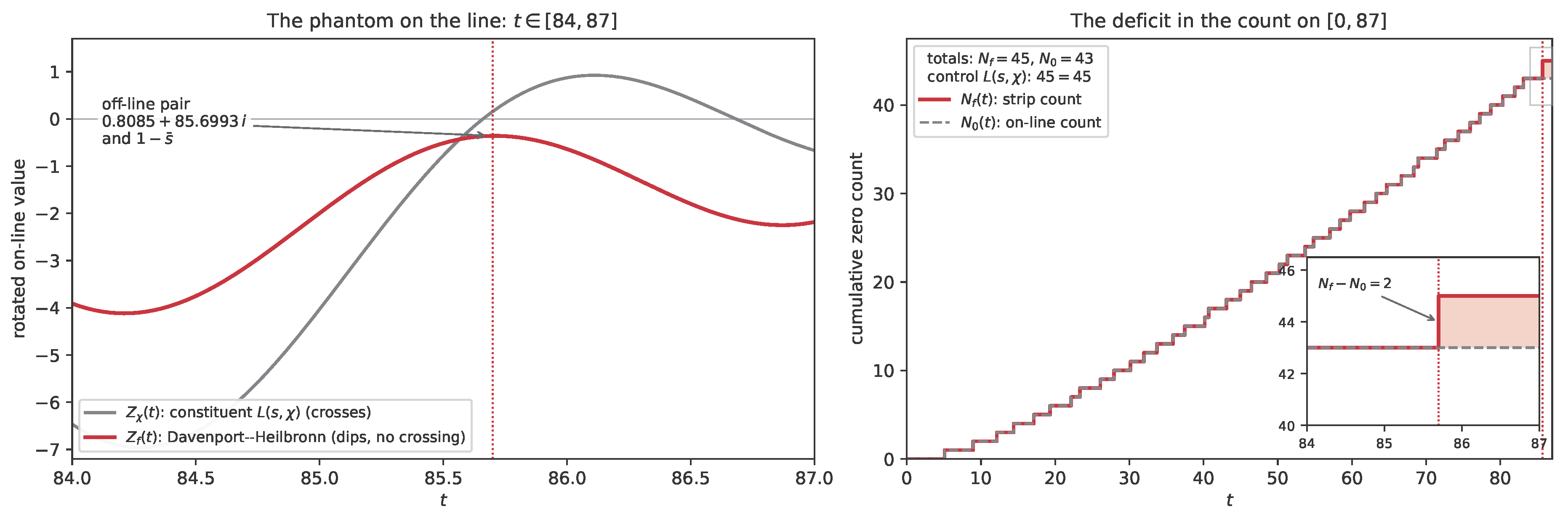
Disclaimer/Publisher’s Note: The statements, opinions and data contained in all publications are solely those of the individual author(s) and contributor(s) and not of MDPI and/or the editor(s). MDPI and/or the editor(s) disclaim responsibility for any injury to people or property resulting from any ideas, methods, instructions or products referred to in the content. |
© 2026 by the authors. Licensee MDPI, Basel, Switzerland. This article is an open access article distributed under the terms and conditions of the Creative Commons Attribution (CC BY) license (http://creativecommons.org/licenses/by/4.0/).
Copyright: This open access article is published under a Creative Commons CC BY 4.0 license, which permit the free download, distribution, and reuse, provided that the author and preprint are cited in any reuse.


