

Submitted:
06 June 2026
Posted:
09 June 2026
You are already at the latest version
Abstract
Cowpea is a crop of great importance worldwide, which is why many heirloom varieties and improved cultivars are explored. Consuming pods and green beans provides vitamins, minerals, and functional components for people with limited access to vegetables. The pods and green beans of these materials have intrinsic characteristics that distinguish them. Therefore, the objective was to adjust machine learning models to identify cowpea from digital images of pods and green beans using artificial intelligence techniques. Digital images of four heirloom Creole of the cowpea genotypes (Sempre Verde, Rabú de tatu, Corujinha, and Paulistinha) and nine cultivars (BRS No-vaera, BRS Olhonegro, BRS Verdejante, BRS Exuberante, BRS Pajeú, BRS Miranda, IPA 206, BRS Tapaihum, and BRS Pingo de Ouro) were processed using four deep learning architectures for feature extraction (vectorization): InceptionV3, SqueezeNet, VGG16, and VGG19. Six machine learning algorithms were evaluated: K-Nearest Neighbors (KNN), Decision Tree, Random Forest (RF), Gradient Boosting (GB), Support Vector Machines (SVM), and Multi-Layer Perceptron (MLP). The MLP (Artificial Neural Network) and SVM models, particularly when integrated with the InceptionV3 embedder, demonstrated superior performance. For pod classification, these models achieved near-perfect performance, with Area Under the Curve (AUC) and Classification Accuracy (CA) of 1.000. For green beans, the MLP maintained high accuracy (CA = 0.977) and better probabilistic calibration (lower Log-Loss) than the SVM. Digital image-based identification associated with machine learning is an efficient, non-destructive approach for the morphological characterization and discrimination of cowpea genotypes, supporting high-throughput phenotyping (HTP) applications.
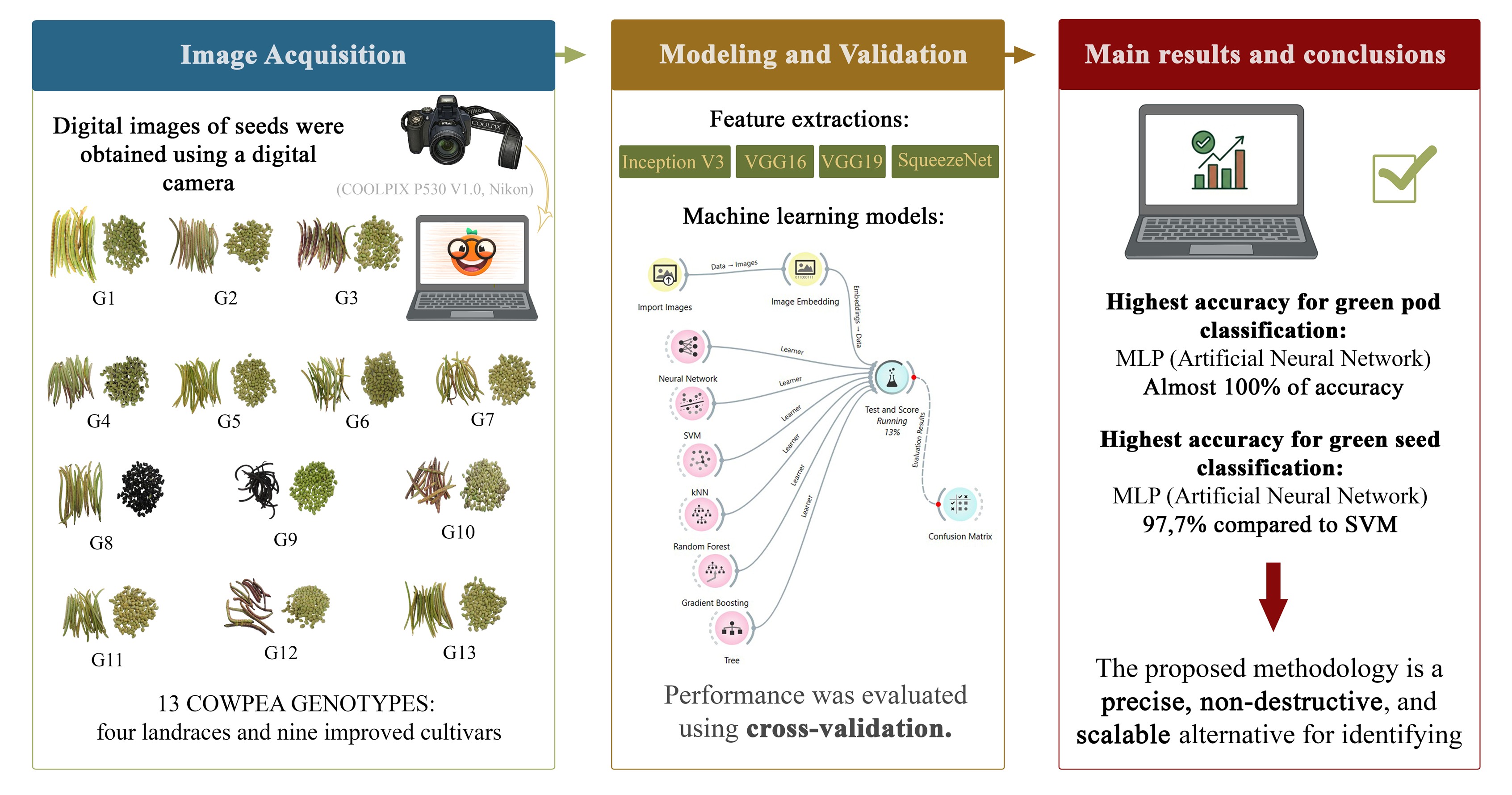
Keywords:
Vigna unguiculata (L.) walp
; artificial intelligence
; artificial neural network
; support vector machine
1. Introduction
Cowpea (Vigna unguiculata [L.] Walp.) is an annual legume native to Africa, recognized for its wide edaphoclimatic adaptability. It is currently cultivated in various regions of America, Asia, and Europe [1]. Cowpea plays a strategic role in food and nutritional security, serving as a primary source of vegetable protein and income for small farmers [2].
Although cowpeas are primarily cultivated for their edible seeds, their young leaves and green pods are often cooked as fresh vegetables. Vegetables are second only to cereals in carbohydrate content; they are rich in dietary fiber and have a high water content, ranging from 70 to 95%. Furthermore, certain vegetables are excellent sources of phosphorus, iron, calcium, potassium, vitamins, and antioxidants. Among these, beans and legumes are commonly consumed worldwide [3,4,5].
Beans are a widely accepted and nutritionally relevant food, standing out as an accessible source of vegetable protein and as an alternative to animal-based proteins. Their nutritional composition includes, in addition to proteins, dietary fiber, carbohydrates, minerals, and vitamins, making them fundamental for food and nutritional security, especially in populations exposed to chronic protein deficiencies [6,7]. Carvalho et al. (2022) [8] evaluated the nutritional composition of immature pods at the stage of complete elongation and found higher levels of proteins, minerals, and phenolic compounds compared to mature beans.
Consuming young green cowpea pods can increase intake of these nutritional and health-promoting components with minimal cooking time, as the pods are softer than mature seeds, thereby minimizing nutrient loss during cooking. A diet rich in beans has several physiological advantages, including the control and prevention of metabolic disorders such as diabetes mellitus, coronary heart disease, and colon cancer [9]
In this context, many genotypes, varieties, lines, and cultivars are explored. Brazil has a wide diversity of cowpea cultivars, developed to meet different edaphoclimatic conditions and exhibiting distinct agronomic characteristics [10]. In addition to commercial cultivars, Brazil possesses a rich diversity of cowpea creole varieties, cultivated and conserved by family farmers over generations, which exhibit wide morpho-agronomic variability, including differences in pod size and shape, grain weight, development cycle, and resistance to environmental stresses [11]. The phenotypic characterization of agricultural cultivars is an essential step in advancing genetic improvement, conserving phytogenetic resources, and developing precision agriculture technologies [12].
Therefore, in the face of advances in digital technologies, automated image-based phenotyping has become an efficient, non-destructive alternative for identifying morphological characteristics. According to [13], the use of vectorizers such as InceptionV3, SqueezeNet, VGG16, and VGG19, combined with machine learning algorithms, enables highly accurate discrimination of cowpea cultivars from digital seed images.
In this scenario, the use of Orange Data Mining software is proposed for the classification of digital images of green pods and grains and the identification of models with greater accuracy and robustness in discriminating between cowpea genotypes, through image vectorization and the application of algorithms such as Artificial Neural Networks (MLP), Support Vector Machines (SVM), Random Forests (RF), and Gradient Boosting (GB).
2. Materials and Methods
2.1. Plant Material
The creole seeds of the cowpea genotypes (Sempre Verde, Rabú de tatu, Corujinha, and Paulistinha) were obtained from a Community Seed Bank of the Queimadas Settlement (7° 08' 27.2" S, 35° 51' 25.2" W), originating from partnerships between AS-PTA Agricultura Familiar e Agroecologia and farmers from the Seed Commission of the Borborema Pole and the Seed Network of the Articulação do Semiárido Paraibano, Lagoa do Jogo site, municipality of Remígio, Paraíba, Brazil.
The seeds of the cowpea varieties (BRS Novaera, BRS Olhonegro, BRS Verdejante, BRS Exuberante, BRS Pajeú, BRS Miranda, IPA 206, BRS Tapaihum, and BRS Pingo de Ouro) were obtained from the germplasm bank of the Brazilian Agricultural Research Corporation, Embrapa Meio-Norte, located in Teresina, Piauí, Brazil (Coordinates: 5°05' S, 42°49' W, Altitude: 72 m).
2.2. Area Characterization and Experimental Conduct
The cultivation of cowpea was carried out under field conditions from March to May 2024, in an agricultural area belonging to the Center for Agricultural and Environmental Sciences (CCAA), on campus II of the State University of Paraíba (UEPB), in Lagoa Seca, Paraíba, Brazil (7º 10' 8" S; 35º 51' 20" W), and an altitude of 634 m. For each genotype, four plots were established, each consisting of four 2 m-long rows spaced 0.5 m apart, with a plot area of 4 m2 and a total area of 16 m2. Sowing was carried out with two seeds per hole, spaced 0.5 m between rows and 0.2 m between plants, resulting in a density of 10 plants per square meter.
The climate, according to the Köppen classification, is type 'AS', tropical with a dry season, with average annual temperatures around 22 °C, a minimum of 19 °C and a maximum of 26 °C, average yearly rainfall above 700 mm, with the highest concentration from April to August; average annual reference evapotranspiration of 500 mm and average annual relative humidity of 80% [14].
The soil in the experimental area is classified as clay loam and has the following characteristics: 86.04% sand, 12.05% silt, and 1.91% clay, characterizing a sandy texture. The bulk density was 1.62 g cm⁻³, the particle density was 2.69 g cm⁻³, and the total porosity was 39.77%. The soil presented the following chemical contents: calcium 1.90 cmolc dm⁻³, magnesium 1.47 cmolc dm⁻³, sodium 0.13 cmolc dm⁻³, potassium 0.28 cmolc dm⁻³, sulfur 3.76 cmolc dm⁻³, hydrogen 1.07 cmolc dm⁻³, and absence of exchangeable aluminum (0.00 cmolc dm⁻³). The organic matter content was 0.91%, and the soil pH was 6.47, determined according to the methodology described by [15].
Meteorological variables were monitored by an automatic station installed 10 m from the experimental area. During the experiment, the average temperature was 23.8 °C, the average relative humidity was 83.37%, and the average accumulated precipitation was 0.57 mm. Irrigation management was carried out daily based on climate monitoring and weather station data. Reference evapotranspiration (ETo) was calculated using the Penman-Monteith method – FAO [16], with the determination of the gross irrigation depth (LB), application intensity (Ia), and irrigation time (Ti).
2.3. Acquisition and Processing of Digital Images
The acquisition and processing of images of green pods and grains were carried out at the Cultivated Plant Ecophysiology Laboratory (ECOLAB), at the State University of Paraíba (UEPB), located in the Três Marias Integrated Research Complex (campus I), in Campina Grande, Paraíba, Brazil (07° 13' 50'' latitude, 35° 52' 52'' longitude and 551 m altitude).
Digital images (n = 25) of the pods and green grains of each cowpea genotype were obtained with a digital camera (Nikon, COOLPIX P530 V1.0), configured with ISO 400, 16 MP resolution (4608 x 3456 pixels), and 300 DPI. The captures were performed in 8-bit RGB mode and stored in JPEG format. The sampling protocol consisted of five images obtained at a zenith angle (90° relative to the ground) and 20 images, captured at 45° angles, directed to the cardinal points (North, South, East, and West), with five repetitions per direction, maintaining a constant focal distance of 1 m.
Image processing was performed using Orange Data Mining software (v. 3.37.0), an open-source platform based on Python and widely used for machine learning and data mining tasks. Its multi-layered architecture allows its use by both novice users and advanced programmers [17]. Orange Data Mining provides a range of components for data preprocessing, feature scoring, and selection, as well as tools for simulation, model evaluation, and data exploration techniques [18].
The image processing workflow followed the steps illustrated in Figure 1. Initially, of the 25 images obtained per genotype or variety, 20 were selected and imported using the 'Import Images' widget of the 'Image Analytics' add-on. Subsequently, the images were processed and vectorized using the 'Image Embedding' widget. This vectorization process was compared with the embedders InceptionV3, SqueezeNet, VGG16, and VGG19 [19].
The adjustment of pod and grain classification models for cowpea genotypes involved testing different machine learning algorithms. Their hyperparameters were iteratively optimized until the best performance indicators were achieved for each model, as detailed below:
K-Nearest Neighbors (kNN): Genotype identification was based on the analysis of the k=5 nearest neighbors. For the calculation of proximity matrices, the Minkowski distance metric with parameter p=2 (equivalent to Euclidean distance) was adopted, applying uniform weights to all points in the neighborhood to ensure that each neighbor contributed equally to the final classification.
Decision Tree: Classification was performed using the C4.5 algorithm. To control model complexity and mitigate overfitting, a minimum limit of two instances per leaf was established, and induction was stopped whenever node purity reached 95%.
Random Forest (RF): The model was configured as an ensemble of 10 independent decision trees. The growth process of each tree was not limited in depth, allowing the algorithm to explore correlations among the features extracted during vectorization exhaustively.
Gradient Boosting (GB): This reinforcement learning method used the Gradient Boosting algorithm (scikit-learn), with 100 trees and a learning rate of 0.100. The maximum depth of the trees was limited to 3 levels to ensure the model's ability to generalize to unseen data.
Support Vector Machine (SVM): This is a machine learning technique that separates the space of different classes. The separation of classes was performed with a marginal cost of C = 1.0 and a regression tolerance of 0.10. The Radial Basis Function (RBF) kernel was used, with the gamma coefficient (ᵞ) configured in 'auto' mode, aiming to find the ideal separation hyperplane in the feature space.
Neural network (MLP - multi-layer perceptron): The Multi-Layer Perceptron neural network was structured with a hidden layer of 100 neurons. The ReLU activation function was adopted in the inner layers, and the Adam optimizer (based on stochastic gradient descent) was used, with a learning rate of 0.001 and a limit of 200 iterations for model convergence.
The performance evaluation of the models was conducted using various sampling methods available in the Orange Data Mining software, including cross-validation, cross-validation by feature, random sampling, leave-one-out validation, and testing on the training data. For final validation and verification of the models' generalization capacity, the test-on-test data method was applied. This step used vectors corresponding to 5 images for each genotype/variety (25 in total, obtained initially), which were kept isolated and did not participate in any adjustment or training steps of the algorithms.
The performance evaluation and final validation of the classification models were based on robust statistical metrics. The indicators used included area under the receiver operating characteristic curve (AUC-ROC), classification accuracy, the weighted harmonic mean of precision and sensitivity (F1-score), and precision, recall, and specificity. Additionally, the Matthews Correlation Coefficient (MCC) and cross-entropy loss (log-loss) were calculated. For computational efficiency analysis purposes, training and test times were also recorded.
3. Results
3.1. Phenotyping of Green Cowpea Pod Varieties
Digital images of green cowpea pods reveal significant morphological variability among the analyzed genotypes (Figure 2). Significant contrasts are observed in morphological attributes such as length, thickness, and degree of curvature (ranging from straight to strongly arched pods). Regarding colorimetry, a wide range of patterns was observed, including uniform green tones, greenish variations with purplish pigmentation, and darker colors. Additionally, variations in surface texture were identified, including longitudinal striations and differences in the degree of morphological uniformity. These phenotypic discrepancies provide a basis for visual features that enable machine learning algorithms to make robust distinctions between genotypes.
The comparative analysis of different classification algorithms for identifying green cowpea pods, using four embedded architectures for feature extraction, is detailed in Table 1. Using InceptionV3 as a feature extractor, the Neural Network (NN) and Support Vector Machine (SVM) models showed the best performance, with maximum metrics (1.000) for the area under the receiver operating characteristic (ROC curve (AUC), classification accuracy (CA), weighted harmonic mean accuracy (F1), precision, recall, Matthews Correlation Coefficient (MCC), and specificity.
Additionally, both exhibited low cross-entropy (log-loss) values of 0.001 and 0.403, respectively. Although the SVM demonstrated predictive effectiveness similar to that of the NN, its training time (TT) was significantly shorter (10.295 s). The kNN algorithm also achieved high performance (AUC of 0.998); however, it showed lower accuracy (0.942) compared to the top-down models. In contrast, the tree-based model (Decision Tree) showed the lowest overall performance (AUC = 0.878; CA = 0.750) and the highest log-loss (8.076), indicating lower predictive reliability.
Gradient Boosting, despite achieving reasonable metrics (AUC = 0.987; CA = 0.896), had the longest training time among all models (1,422,669 s), which may limit its applicability in systems with computational constraints.
The SqueezeNet architecture demonstrated remarkable performance as a feature extractor, especially when integrated with Neural Network (NN) and Support Vector Machine (SVM) classifiers. Both models achieved metrics close to unity across all indicators, including AUC-ROC, accuracy (CA), F1-score, precision, sensitivity, and specificity, demonstrating high discriminative power and a balanced class distribution. The log-loss values obtained (0.008 for NN and 0.394 for SVM) reinforce the robustness of the predictions, indicating low penalty and a high probability of success.
Random Forest also showed stability (AUC = 0.999; CA = 0.965), with a marginal increase in log-loss (0.449). In contrast, the Decision Tree model showed the lowest overall performance (AUC = 0.872; CA = 0.746) and the highest log-loss (8.484). Finally, kNN stood out for its computational speed (TT = 2.269 s). At the same time, Gradient Boosting, despite its strong predictive performance (AUC = 0.996), incurred a significantly higher computational cost (TT = 830.300 s) than other models in the same class.
When using VGG16 as a feature extractor, both NN and SVM demonstrated superiority, with metrics close to perfect. The NN model achieved unit results across all indicators (AUC-ROC, CA, F1-score, MCC, and specificity = 1.000) and the lowest log-loss (0.001). However, it required high training (TT) and testing times (36.035 s and 12.437 s, respectively). SVM showed comparable performance (AUC = 0.999; CA = 0.962), with a log-loss of 0.461. Random Forest also demonstrated excellent adaptability to VGG16, achieving an accuracy of 0.992 and a low log-loss (0.354).
On the other hand, Gradient Boosting, despite achieving a competitive accuracy (CA = 0.954), had the longest training time in the study (1,364.514 s), suggesting limitations for real-time applications or those with hardware constraints. The tree-based model (Decision Tree) showed the worst overall performance (CA = 0.831; log-loss = 5.575), while kNN showed intermediate results (CA = 0.954; log-loss = 0.257), although it was inferior to those of more robust models.
The use of VGG19 as an embedder underscored the superiority of NNs and SVMs, with their metrics approaching perfection. Notably, the NN model achieved the highest performance (1.000 across all indicators), registering the lowest log-loss in the study (0.000), although it required the longest processing time (TT = 40.057 s; Test Time = 15.503 s). SVM presented comparable results (CA = 0.981; F1-score = 0.985) and a training time of 24.156 s. Random Forest demonstrated its efficiency and a balanced trade-off between precision and computational cost (CA = 0.988; F1-score = 0.989).
In contrast, Gradient Boosting, despite its satisfactory predictive performance (AUC = 0.997), had the longest training time (1,727.015 s), underscoring its impracticality in hardware-constrained scenarios. Finally, the Decision Tree model replicated the low-performance pattern observed in the other extractors (CA = 0.819; log-loss = 6.249), while kNN maintained an intermediate performance level (CA = 0.946).
The Neural Network (NN) and Support Vector Machine (SVM) models showed high performance with all embedders. The Neural Network performed best with all embedders, with metrics close to 1. The Inception V3 embedder achieved the best metric among the Neural Network models and had the lowest training and testing times. Given the optimal parameters, the Inception V3 embedder was chosen.
The confusion matrix (Table 2) details the performance of the Neural Network (NN) model with the InceptionV3 embedder in classifying green pods of 13 cowpea genotypes. The model achieved perfect accuracy (100%) in 12 of the 13 materials evaluated, with all samples correctly assigned to their respective classes. Only one classification error was observed in the Sempre Verde cultivar (G13), where a sample was incorrectly labeled as BRS Pajeú (G5). The absolute predominance of predictions on the main diagonal of the matrix confirms the model's effectiveness in discriminating genotypes, even among those with similar morphological characteristics. These results consolidate the robustness of InceptionV3 in feature extraction and the high precision of Neural Networks in precision digital phenotyping applications.
The comparative analysis of the activation functions (Table 3) demonstrated that ReLU, in conjunction with the L-BFGS-B optimizer, showed superior performance, reaching the unitary level (1,000) in all classification metrics. This combination resulted in a very low log-loss, highlighting the model's robustness and the consistency of its predictions. Although the Logistic and Hyperbolic Tangent (tanh) functions presented satisfactory results, a slight degradation in accuracy and an increase in classification error were observed when associated with the SGD (Stochastic Gradient Descent) algorithm.
In contrast, the Identity function showed the lowest overall performance, attributable to its inability to model the complex nonlinear relationships inherent in pod morphology. Therefore, the combination of ReLU with L-BFGS-B proved to be the ideal configuration, offering the best balance between predictive effectiveness, convergence stability, and mitigation of overfitting.
The confusion matrix obtained for the NN configured with the ReLU activation function and the L-BFGS-B optimizer showed absolute performance in classifying the 13 cowpea genotypes (Table 4). All classes registered 20 correct classifications, with no false positives or negatives. This result indicates that the attributes extracted by the model were highly discriminative, enabling a clear, linear, or non-linear separation between the classes in the feature space. Although the ideal performance validates the effectiveness of the proposed architecture, it also reinforces the need for future tests on external datasets (external validation) to ensure the model's robustness and rule out potential overfitting.
The comparison between the different embedders and classifiers (Table 5) indicates that the SVM and v-SVM (linear, polynomial, and RBF kernels) obtained superior performance metrics (AUC, accuracy, F1-score, and MCC), demonstrating high discriminatory capacity. However, the high LogLoss values suggest poor probabilistic calibration: although the classifications are mostly correct, the model is overconfident in its inaccurate predictions. Therefore, the selection of the ideal model should balance classification effectiveness with the reliability of the estimated probabilities, prioritizing configurations that minimize LogLoss.
The confusion matrix (Table 6) of the SVM classifier with a linear kernel confirms that, despite satisfactory overall performance, classification errors persist in specific classes. It is noted that, while most cultivars were accurately identified, specific genotypes showed overlap (misclassification), with samples incorrectly assigned to similar courses. These results indicate that linear separation in the extracted feature space is insufficient to discriminate among all varieties, suggesting the presence of complex morphological patterns that require non-linear decision functions or models with greater representational capacity.
3.2. Model Validation
The performance metrics for the Neural Network (Table 7) and SVM (Table 8), evaluated using an additional validation dataset of cowpea pod images, yielded ideal classification results. Both models achieved scores of 1.000 across all metrics, including AUC, CA, F1-score, Precision, Recall, and MCC. These results demonstrate full generalization capacity and robustness when processing unseen data, confirming that the digital features extracted from pods are highly discriminative against the analyzed genotypes.
In the comparative evaluation, both the Neural Network (Table 9) and the SVM (Table 10) achieved peak performance across all global metrics, with AUC, CA, F1-score, and MCC values of 1.000. Nevertheless, an analysis of the confusion matrices reveals critical distinctions in their predictive behavior. The Neural Network delivered deterministic and highly confident classifications, with all samples concentrated along the main diagonal. Conversely, the SVM exhibited a less robust probabilistic calibration; although the final predictions were 100% accurate, the model assigned residual probabilities (0.1 to 0.3) to incorrect classes outside the diagonal. This suggests that, unlike the Neural Network, the SVM operated with a lower confidence margin, distributing probability mass across neighboring classes despite achieving the correct final classification.
3.3. Phenotyping of Green Cowpea Genotypes
Phenotyping of green cowpea varieties (Figure 3) indicates high phenotypic diversity among genotypes. Consistent variations are observed in morphological and chromatic attributes, including dimensions (size and rounded or elongated shape), seed coat shades, and distinct hilum patterns. Furthermore, heterogeneity in surface texture and batch uniformity reflects specific genotypic traits. These visual contrasts provide fundamental discriminating attributes, which were extracted and processed by machine learning models to enable accurate classification of the materials.
Table 11 demonstrates that, using the InceptionV3 embedder, the Neural Network and SVM models were the most effective, both achieving an AUC of 1.000 and a CA of 0.977. However, the Neural Network achieved a significantly lower LogLoss (0.075) than the SVM (0.413), indicating superior probabilistic calibration. The kNN model had intermediate performance (CA = 0.892), while the Gradient Boosting and Random Forest models showed lower accuracies and higher LogLoss, reflecting greater predictive uncertainty. The Decision Tree model was the least efficient (CA = 0.681; LogLoss = 10.586). Therefore, for green grain classification, the Neural Network may be the preferred option due to the balance between precision and reliability. At the same time, the SVM is a robust alternative, although less calibrated.
The results obtained with the SqueezeNet embedder confirm the superiority of the Neural Network and the SVM. Both achieved high performance metrics, with AUCs of 0.998 and 0.995 and a CA of 0.962, demonstrating consistent recognition of green grain classes. However, the Neural Network's LogLoss (0.204) was significantly lower than the SVM's (0.497), indicating superior probabilistic calibration despite similar classification performance. The kNN showed intermediate performance (CA = 0.865), while Gradient Boosting and Random Forest obtained lower results. The Decision Tree model showed limited effectiveness (CA = 0.581; LogLoss = 13.79). Thus, as observed with InceptionV3, the Neural Network consolidates itself as the most suitable model when using SqueezeNet, harmonizing high accuracy with greater predictive reliability.
Using VGG16 as a feature extractor, the Neural Network again demonstrated superior overall performance, with an AUC of 0.998 and a CA of 0.962, accompanied by a low LogLoss (0.204), ensuring robust calibration. The SVM achieved identical classification metrics (CA = 0.962) but a higher LogLoss (0.493), indicating greater predictive uncertainty than the Neural Network. Ensemble Learning models, such as Gradient Boosting and Random Forest, showed intermediate performance, while the kNN showed reduced effectiveness. The Decision Tree model consistently obtained the lowest performance, with a critical LogLoss of 13.379. This evidence confirms that the Neural Network is the most consistent and reliable classifier among the embedders tested, closely followed by the SVM.
Using the VGG19 embedder, the Neural Network maintained outstanding performance, with an AUC of 0.978 and a CA of 0.977, achieving the lowest LogLoss (0.122) among all models and demonstrating superior probabilistic calibration and reliability. The SVM achieved slightly superior classification accuracy (CA = 0.985) but a considerably higher LogLoss (0.436), indicating greater uncertainty in the predicted probabilities. Models such as Gradient Boosting and Random Forest achieved intermediate performance, while kNN achieved lower performance. Once again, the Decision Tree model was the least efficient (CA = 0.681). These results reinforce the Neural Network's consistency as the most robust model from a calibration perspective, followed by the SVM.
Neural Network and Support Vector Machine (SVM) models demonstrated superior performance in all embedders tested for identifying green cowpea grains. The Neural Network outperformed the other classifiers, regardless of the feature extraction architecture, achieving its maximum performance when combined with InceptionV3, with the lowest recorded LogLoss index (0.075). Consequently, the InceptionV3 extractor was selected as the ideal architecture for this phenotyping system due to its superior balance between classification accuracy and probabilistic reliability.
The confusion matrix generated by the Neural Network with the InceptionV3 extractor (Table 12) demonstrates superior performance in classifying green grains from 13 cowpea genotypes. Most genotypes were correctly identified, with values close to the total number of instances per class (20), with BRS Verdejante, Corujinha, and Rabo de Tatu standing out, achieving full classification (20.0). Slight discrepancies were observed between morphologically similar genotypes, such as BRS Pajeú and Paulistinha, which exhibited mutual overlap (1.3 and 1.9 instances, respectively). Despite these marginal discrepancies, the robustness of the model is supported by high overall indices (CA = 0.977; AUC = 1.000), confirming the effectiveness of the InceptionV3 architecture, combined with neural networks, for accurate phenotyping of the evaluated genotypes.
The performance metrics of the Artificial Neural Network with the InceptionV3 extractor (Table 13) revealed high robustness in all combinations of activation functions and solvers. The L-BFGS-B solver showed superior results, particularly with the Tanh and ReLU functions, achieving an AUC of 1.000 and a CA of 0.977, along with the lowest LogLoss values (0.061 and 0.075, respectively), demonstrating excellent predictive stability. The SGD solver showed inferior performance, especially in the Logistic function (CA = 0.892; LogLoss = 0.918). On the other hand, the Adam solver showed intermediate effectiveness, with emphasis on the Logistic function (CA = 0.981; LogLoss = 0.090). Therefore, the results confirm that the synergy between InceptionV3 and MLP is consistent, with the combination of the L-BFGS-B solver with the ReLU activation function being the most efficient for the proposed phenotyping.
The confusion matrix of the Artificial Neural Network, configured with the ReLU activation function and the L-BFGS-B solver (Table 14), showed results consistent with the previously observed overall performance. This stability demonstrates that the choice of these specific hyperparameters ensures maximum accuracy in classifying varieties, without degrading predictive metrics.
The performance metrics of the SVM algorithm (Table 15) under different kernel functions demonstrate that the Linear and Polynomial kernels were the most effective. Both achieved maximum performance (AUC = 1.000; CA = 0.977; F1 = 0.977), with LogLoss values of 0.408 and 0.400, respectively. The RBF kernel showed slightly lower effectiveness (CA = 0.954), while the Sigmoid kernel showed the lowest performance, with sharp reductions in accuracy (CA = 0.769) and the highest LogLoss (1.035), indicating predictive instability. Analogous results were obtained with v-SVM, reaffirming the superiority of the Linear and Polynomial kernels. Therefore, the polynomial kernel in the SVM algorithm has proven to be the best choice for this model.
The SVM confusion matrix with a polynomial kernel (Table 16) shows consistent performance in classifying green grain genotypes. Residual confusion rates are observed between specific classes (e.g., G6 and G5; G7 and G6; G13 and G12), suggesting overlap in morphological characteristics within the representations extracted by the embedder. Nevertheless, the incidence of errors remains marginal relative to the total number of samples, confirming the robustness of the polynomial kernel compared with the other basis functions tested. These results confirm the high CA, F1-score, and MCC values, consolidating the polynomial kernel as the optimal configuration for this classification scenario.
3.4. Validation for Green Cowpea Seeds
The results obtained by the Artificial Neural Network in the validation stage (Table 17) indicate robust and consistent performance. The AUC value (1.000) indicates the maximum discriminative power between classes. The accuracy (0.923) and the F1-score (0.889) indicate a satisfactory balance between precision and sensitivity (recall). Evidently, the model achieved perfect precision (1.000), indicating no false positives, while the recall of 0.800 suggests that a fraction of positive instances were not captured. The MCC of 0.917 reinforces the high quality of the overall classification, confirming the model's reliability even in the face of a slight disparity between omission and inclusion errors.
The confusion matrix for the Artificial Neural Network during the validation stage (Table 18) shows robust performance, with most values on the main diagonal. In most classes (G1 to G13), the model achieved full classification (5/5), demonstrating high accuracy. Discrete deviations were observed in cultivars such as G2, G5, G7, G11, and G13, in which minimal fractions of instances were permuted. However, the overall consistency of the matrix confirms the network's excellent generalization capacity, consistent with the previously discussed performance indicators (AUC = 1.000; CA = 0.923; MCC = 0.917).
The results from the SVM algorithm's validation stage (Table 19) confirm its high predictive performance. The model achieved an AUC of 1.000, indicating perfect separation between classes, and maximum values (1.000) for F1-score, precision, and recall, with no classification errors across these metrics. The accuracy (CA = 0.954) and the Matthews Correlation Coefficient (MCC = 0.951) reinforce the model's consistency, highlighting the robustness of the SVM in the face of the variability of the cowpea genotypes evaluated.
The confusion matrix for the SVM algorithm validation (Table 20) reveals a more pronounced dispersion of errors. In several classes, the values are distributed across multiple columns, indicating instability in variety classification. For example, in G1, only 2.9 instances were correctly classified, while 2.1 were erroneously assigned to other classes. This scenario demonstrates that, although global metrics such as F1-score and Recall have nominal values of 1.000, the predictive consistency at the class level is lower than that of the Neural Network, evidencing a lower generalization capacity of the SVM for this specific dataset.
4. Discussion
The results of this study confirm that integrating feature extractors based on pre-trained convolutional neural networks (embedders) with supervised classifiers constitutes a robust strategy for genotyping cowpea from digital images. Specifically, the synergy between the Multi-Layer Perceptron (MLP) classifier and the InceptionV3 embedder demonstrated an ideal balance among classification accuracy, probabilistic calibration (LogLoss), and resilience to phenotypic variability across genotypes. These results confirm the advantages of multiscale architectures, inherent in Inception modules, for capturing complex patterns in high-precision digital phenotyping tasks [20,21].
In the present study, both Neural Networks and SVM achieved overall metrics exceeding 95%, a level considered excellent for digital phenotyping. However, detailed analysis of the confusion matrices and LogLoss revealed critical divergences. While the SVM produced correct final decisions, it exhibited poor calibration in assigning probability fractions across adjacent classes, indicating reduced predictive confidence. In contrast, the Neural Network provided more deterministic and better-calibrated predictions (lower LogLoss). This superiority in probabilistic calibration, combined with high accuracy, corroborates recent methodological recommendations emphasizing the need to evaluate the interpretability of models' confidence, beyond traditional metrics such as AUC and F1-score [22,23].
These results reinforce the idea that computer vision-based cultivar identification has transformed feature extraction and the analysis of large volumes of visual data, enabling integration into genetic improvement pipelines and high-throughput phenotyping (HTP). In this context, deep learning architectures, such as Inception, ResNet, and DenseNet, often outperform classical machine learning approaches in agricultural classification tasks. This is because such networks learn rich, multiscale representations that are fundamental for discriminating between morphologically similar classes, such as those of the cowpea genotype analyzed [24,25].
In this sense, the ability of deep architectures to extract rich, multiscale representations that surpass classical machine learning approaches establishes a solid foundation for their incorporation into precision agriculture systems. The integration between computer vision and machine learning algorithms, as demonstrated in this study, broadens the application horizon of these tools in genetic improvement programs, the conservation of plant genetic resources, and the development of intelligent decision support systems (DSS). Such advances are fundamental to promoting sustainable, technological production of cowpea [26].
The selection of the optimization configuration and activation functions was decisive; the combination of ReLU with the L-BFGS-B solver achieved stable convergence and superior performance across all evaluated metrics. Recent optimization studies indicate that variants of the Quasi-Newton method (such as L-BFGS) can accelerate convergence and improve stability in moderately large networks, especially in controlled phenotyping datasets that do not reach massive scales. Therefore, the exploration of second-order solvers is recommended when computational cost permits, to achieve greater accuracy and stability in training [27,28].
In decision tree-based classifiers and certain ensembles, performance was inferior to that of algorithms that better exploit the non-linear representations generated by CNNs. This suggests that for high-dimensional vectors with strong attribute interactions, as in image embeddings, models with greater approximation capabilities, such as Deep Neural Networks and SVMs with suitable kernels, extract the available information more efficiently. Similar results were reported by [29] and [21], who also identified limitations of tree-based methods for plant target detection and classification.
In the specific context of cowpea (Vigna unguiculata), recent advances have significantly expanded the available genetic and phenotypic resources, ranging from genome-wide association studies (GWAS) to the construction of robust image databases [30]. These advances reinforce the potential of integrating image-based phenotyping and genomic data to accelerate genetic progress. The identification of molecular markers and quantitative trait loci (QTLs) associated with pod and grain attributes enhances the applicability of automated classification systems, especially in rapid germplasm screening and decision support in assisted selection programs [31]
Despite the high performance achieved by the evaluated models, especially in the combination of Inception V3 and Neural Network, some limitations and future directions should be considered to enhance the robustness, applicability, and scientific impact of the proposed approach. The images used in this study were acquired under control conditions, which may favor model performance but may not fully reflect the variability present in real agricultural environments, such as variations in lighting and background, the presence of impurities, physical damage, and different stages of grain and pod maturation. Recent evidence indicates that models trained exclusively in standardized scenarios may degrade in performance when applied to field conditions, making it essential to expand and diversify the image bank with data from real environments to ensure model generalization and effective technology transfer.
Additionally, although the number of genotypes evaluated is representative, including a broader set of cultivars and additional growing seasons could yield a more comprehensive assessment of the models' robustness. Finally, the strategy based on pre-trained embeddings, while efficient, does not fully exploit the potential of deep architectures trained end-to-end, which may limit the capture of specific phenotypic patterns of cowpea. These limitations, however, do not compromise the study's conclusions but point to clear opportunities for future investigations.
Another promising perspective is the integration of image-based phenotyping with genomic data, such as molecular markers, QTLs, and genome-wide association studies (GWAS). In the context of cowpea, recent advances in genomics have provided resources that enable the association of pod and grain visual characteristics with specific genomic regions. The fusion of machine learning, digital imaging, and genomics can significantly accelerate breeding programs by enabling indirect selection of superior genotypes based on highly heritable visual phenotypes.
Future research could explore end-to-end deep learning strategies, in which the CNN simultaneously performs feature extraction and classification, eliminating the separation between the embedder and the classifier. While this approach requires larger datasets, it can capture even more complex relationships between morphological patterns and genotypes. Alternatively, lighter architectures, such as MobileNet and EfficientNet, could be evaluated for applications in mobile devices and embedded systems, which is particularly relevant for field use in the Brazilian Semi-Arid region.
The incorporation of explainable learning techniques represents another important frontier. Methods such as Grad-CAM, LIME, or SHAP, applied to agricultural images, allow the identification of which pod or grain regions are most relevant to the model's decision. This not only increases transparency and confidence in the prediction but also reveals discriminating phenotypic characteristics that remain underexplored by traditional visual taxonomy, thereby contributing to the definition of new selection criteria in breeding programs.
Future research could investigate the use of semi-supervised or self-supervised learning to reduce reliance on large volumes of labeled data, a recurring challenge in germplasm banks. These approaches have shown promising results in recent literature on computer vision applied to agriculture, especially in scenarios with multiple classes and genotype-limited samples. Furthermore, it is recommended to evaluate model performance across different growing seasons and environments, accounting for genotype-environment interactions. The ability to consistently distinguish genotypes under abiotic stresses, such as water deficits and high temperatures, which are typical in the semi-arid region, can substantially increase the methodology's agronomic relevance. Thus, the continuation of this work can contribute not only to methodological advances in artificial intelligence applied to agriculture but also to the development of more adapted and resilient cowpea cultivars.
5. Conclusions
This study confirms that image-based digital identification, integrated with machine learning algorithms, is an efficient and non-destructive method for identifying and morphologically characterizing cowpea genotypes using pods and green beans.
Feature extraction using neural network embedders, processed in the Orange Data Mining software, achieved high predictive performance in complex multiclass scenarios.
The Artificial Neural Network showed the most robust performance, with superior accuracy metrics, F1-score, and MCC. The confusion matrix analysis validated the model's high discriminative capacity, reinforcing that the MCC and F1-score are more accurate indicators for evaluating performance under class-imbalance conditions.
The results confirm the potential of integrating computer vision and machine learning as a tool to support precision agriculture. This approach has direct applications in plant breeding programs, germplasm conservation, and the development of intelligent decision support systems for the sustainable production of cowpea.
Author Contributions
Conceptualization, S.I.B., C.A.V.d.A., A.S.d.M., and R.L.d.S.F.; methodology, validation, investigation, and formal analysis, G.F.D., A.M.F.d.O., P.M.d.O.V., I.E.C., R.A.M.L., and A.C.d.S.D.; writing—original draft, S.I.B., A.M.F.d.O., R.L.d.S.F., H.A.d.A., F.V.d.S.S., A.S.d.M. and C.A.V.d.A.; writing—review & editing, S.I.B., A.M.F.d.O., R.L.d.S.F., H.A.d.A., F.V.d.S.S., A.S.d.M. and C.A.V.d.A.; supervision, R.L.d.S.F., A.S.d.M. and C.A.V.d.A.; project administration, R.L.d.S.F., A.S.d.M. and C.A.V.d.A.; All authors have read and agreed to the published version of the manuscript.
Funding
There was no funding.
Data Availability Statement
The raw data supporting the conclusions of this article will be made available by the authors on request.
Acknowledgments
The authors would like to extend their sincere appreciation to the Coordenação de Aperfeiçoamento de Pessoal de Nível Superior (CAPES), financial code 001, and the Programa Institucional de Pós-Doutorado (PIPD – CAPES) (Proc. 88887.081429/2024-00). To the Postgraduate Program in Agronomy - PPGAgro. À Universidade Federal da Paraíba (UFPB). To the Seed Analysis Laboratory (LAS). The Conselho Nacional de Desenvolvimento Científico e Tecnológico (CNPq) for the granting of financial aid (Proc. 408952/2021-0 e 307559/2022-0). The Fundação de Apoio à Pesquisa do Estado da Paraíba (FAPESP/PB) (Edital FAPESP/PB/CNPq nº 77/2022). The INCT em Agricultura Sustentável no Semiárido Tropical - INCTAGriS (CNPq/Funcap/Capes). The Universidade Estadual da Paraíba (UEPB) and the Laboratório de Ecofisiologia de Plantas Cultivadas (Ecolab) for awarding grants to the researchers. During the preparation of this manuscript/study, the author(s) used ChatGPT 4.0 to create the flowchart shown in Figure 1. The authors reviewed and edited the results and assume full responsibility for the content of this publication.
Conflicts of Interest
The authors declare no conflicts of interest.
References
- Nounagnon, M.; Roko, G.; Agbodjato, N.A.; Dah-Nouvlessounon, D.; Babalola, O.O.; Baba-Moussa, L. Cowpea (Vigna unguiculata). Potential Pulses Genet. Genom. Resour. 2024, 58–77. [Google Scholar]
- Ishikawa, H.; Matsumoto, R.; Iseki, K. Changes in folic acid, phenolic components, and angiotensin-converting enzyme inhibitory activity in cowpea (Vigna unguiculata) green pods with different pod maturity. Sci. Prog. 2025, 108, 00368504251320163. [Google Scholar] [CrossRef]
- Sui, W.; Wang, S.; Chen, Y.; Li, X.; Zhuang, X.; Yan, X.; Song, Y. Insights into the structural and nutritional variations in soluble dietary fibers in fruits and vegetables influenced by food processing techniques. Foods 2025, 14, 1861. [Google Scholar] [CrossRef]
- Pandey, A.K.; Shrivastava, A.; Vashishth, R.; Chauhan, O.P. Structure and composition of fruits and vegetables. In Fruits and Vegetables Technologies: Postharvest Processing and Packaging; Springer Nature Singapore: Singapore, 2025; pp. 1–29. [Google Scholar]
- Lisciani, S.; Marconi, S.; Le Donne, C.; Camilli, E.; Aguzzi, A.; Gabrielli, P.; Gambelli, L.; Kunert, K.; Marais, D.; Vorster, B.J.; Alvarado-Ramos, K.; Reboul, E.; Cominelli, E.; Preite, C.; Sparvoli, F.; Losa, A.; Sala, T.; Botha, A.-M.; Ferrari, M. Legumes and common beans in sustainable diets: Nutritional quality, environmental benefits, spread and use in food preparations. Front. Nutr. 2024, 11, 1385232. [Google Scholar] [CrossRef] [PubMed]
- Siddiq, M.; Uebersax, M.A.; Siddiq, F. Global production, trade, processing and nutritional profile of dry beans and other pulses. Dry. Beans Pulses Prod. Process. Nutr. 2022, 1–28. [Google Scholar]
- Kamboj, R.; Nanda, V. Proximate composition, nutritional profile, and health benefits of legumes—A review. Legume Res. 2018, 41, 325–332. [Google Scholar]
- Carvalho, M.; Carnide, V.; Sobreira, C.; Castro, I.; Coutinho, J.; Barros, A.; Rosa, E. Cowpea immature pods and grains evaluation: An opportunity for different food sources. Plants 2022, 11, 2079. [Google Scholar] [CrossRef] [PubMed]
- Islam, S.S.; Adhikary, S.; Mostafa, M.; Hossain, M.M. Vegetable beans: Comprehensive insights into diversity, production, nutritional benefits, sustainable cultivation and future prospects. Online J. Biol. Sci. 2024, 24, 477–494. [Google Scholar] [CrossRef]
- Franco, A.A.N.; Okumura, R.S.; Carvalho, A.J.; Moura Rocha, M.; Ormond, A.T.S.; Cogo, F.D.; Queiroz, M.G.; Oliveira, S.M.; Mariano, Cinque. Agronomic performance of cowpea cultivars in first crop in Southwest of Minas Gerais, Brazil. Cad. Pedagógico 2024, 21, e5819. [Google Scholar] [CrossRef]
- Morais, J.V.S.; Silva, I.R.; Brito, R.R.; Ribeiro, G.S.; Miranda, R.S.; Morais, E.M.; Oliveira, R.I.; Pavan, B.E.; Cunha, J.G.; Silva, L.B. Physiological adjustments in heirloom cowpea under water stress: Effects of rice husk biochar as a silicon source. Int. J. Agron. 2025, 2025, 1731831. [Google Scholar] [CrossRef]
- Roychowdhury, R.; Ghatak, A.; Kumar, M.; Samantara, K.; Weckwerth, W.; Chaturvedi, P. Accelerating wheat improvement through trait characterization: Advances and perspectives. Physiol. Plant. 2024, 176, e14544. [Google Scholar] [CrossRef]
- Megalingam, R.K.; Menon, G.G.; Binoj, S.; Sai, D.A.; Kunnambath, A.R.; Manoharan, S.K. Cowpea leaf disease identification using deep learning. Smart Agric. Technol. 2024, 9, 100662. [Google Scholar] [CrossRef]
- Alvares, C.A.; Stape, J.L.; Sentelhas, P.C.; Gonçalves, J.L.M.; Sparovek, G. Köppen’s climate classification map for Brazil. Meteorol. Z. 2013, 22, 711–728. [Google Scholar] [CrossRef]
- Teixeira, P.C.; Donagemma, G.K.; Fontana, A.; Teixeira, W.G. Manual de Métodos de Análise de Solo, 3rd ed.; Embrapa: Brasília, Brazil, 2017; 574 p. [Google Scholar]
- Allen, R.G.; Pereira, L.S.; Raes, D.; Smith, M. Crop Evapotranspiration: Guidelines for Computing Crop Water Requirements; FAO Irrigation and Drainage Paper 56; FAO: Rome, Italy, 1998; p. 300p. [Google Scholar]
- Demšar, J.; Curk, T.; Erjavec, A.; Gorup, C.; Hočevar, T.; Milutinovič, M.; Možina, M.; Polajnar, M.; Toplak, M.; Starič, A.; Stajdohar, M.; Umek, L.; Žagar, L.; Zbontar, J.; Žitnik, M.; Zupan, B. Orange: Data mining toolbox in Python. J. Mach. Learn. Res. 2013, 14, 2349–2353. [Google Scholar]
- Klunnikova, Y.V.; Anikeev, M.V.; Filimonov, A.V.; Kumar, R. Machine learning application for prediction of sapphire crystals defects. J. Electron. Sci. Technol. 2020, 18, e100029. [Google Scholar] [CrossRef]
- Godec, P.; Pančur, M.; Ilenič, N.; Čopar, A.; Stražar, M.; Erjavec, A.; Pretnar, A.; Demšar, J.; Starič, A.; Toplak, M.; Žagar, L.; Hartman, J.; Wang, H.; Bellazzi, R.; Petrovič, U.; Garagna, S.; Zuccotti, M.; Park, D.; Shaulsky, G.; Zupan, B. Democratized image analytics by visual programming through integration of deep models and small-scale machine learning. Nat. Commun. 2019, 10, 4551. [Google Scholar] [CrossRef] [PubMed]
- Diallo, R.; Edalo, C.; Awe, O.O. Machine learning evaluation of imbalanced health data: A comparative analysis of balanced accuracy, MCC, and F1 score. In Practical Statistical Learning and Data Science Methods: Case Studies from LISA 2020 Global Network; Springer Nature Switzerland: Cham, Switzerland, 2024; pp. 283–312. [Google Scholar]
- Murphy, K.M.; Ludwig, E.; Gutierrez, J.; Gehan, M. Deep learning in image-based plant phenotyping. Annu. Rev. Plant Biol. 2024, 75, 771–795. [Google Scholar] [CrossRef]
- Farhadpour, S.; Warner, T.A.; Maxwell, A.E. Selecting and interpreting multiclass loss and accuracy assessment metrics for classifications with class imbalance: Guidance and best practices. Remote Sens. 2024, 16, 533. [Google Scholar] [CrossRef]
- Wang, C. Calibration in deep learning: A survey of the state-of-the-art. arXiv 2023, arXiv:2308.01222. [Google Scholar]
- Saleem, M.H.; Potgieter, J.; Arif, K.M. Plant disease classification: A comparative evaluation of convolutional neural networks and deep learning optimizers. Plants 2020, 9, 1319. [Google Scholar] [CrossRef]
- Maraveas, C. Image analysis artificial intelligence technologies for plant phenotyping: Current state of the art. AgriEngineering 2024, 6, 3375–3407. [Google Scholar] [CrossRef]
- Livieris, I.E. An advanced active set L-BFGS algorithm for training weight-constrained neural networks. Neural Comput. Appl. 2020, 32, 6669–6684. [Google Scholar] [CrossRef]
- Vickers, P.; Barrault, L.; Monti, E.; Aletras, N. We need to talk about classification evaluation metrics in NLP. arXiv 2024, arXiv:2401.03831. [Google Scholar] [CrossRef]
- Wang, Y.; Han, Y.; Wang, C.; Song, S.; Tian, Q.; Huang, G. Computation-efficient deep learning for computer vision: A survey. Cybern. Intell. 2024, 1, 9390002. [Google Scholar] [CrossRef]
- Mostafa, S.; Mondal, D.; Panjvani, K.; Kochian, L.; Stavness, I. Explainable deep learning in plant phenotyping. Front. Artif. Intell. 2023, 6, 1203546. [Google Scholar] [CrossRef]
- Hasan, M.; Muda, N.R.S. Design and develop autonomous 3 in 1 agricultural robots for farming. Int. J. IJNRSM 2024, 4, 56–65. [Google Scholar]
- Shafighfard, T.; Kazemi, F.; Bagherzadeh, F.; Mieloszyk, M.; Yoo, D.Y. Chained machine learning model for predicting load capacity and ductility of steel fiber–reinforced concrete beams. Comput.-Aided Civ. Infrastruct. Eng. 2024, 39, 3573–3594. [Google Scholar] [CrossRef]
Figure 1.
Flowchart of the steps for importing and vectorizing images of pods and green beans of cowpea genotypes in the Orange software.
Figure 1.
Flowchart of the steps for importing and vectorizing images of pods and green beans of cowpea genotypes in the Orange software.
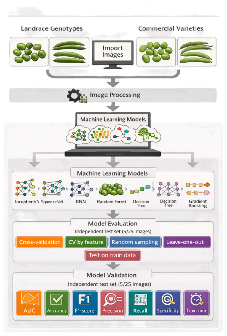
Figure 2.
Morphological variability of green cowpea pods (Vigna unguiculata L. Walp). (G1–G5, G7–G9, G11) Improved cultivars exhibiting predominant uniform green coloration and rectilinear shape: BRS Exuberante, BRS Miranda, BRS Novaera, BRS Olhonegro, BRS Pajeú, BRS Pingo de Ouro, BRS Tapaihum, BRS Verdejante, and IPA 206. (G6, G10, G12, G13) Landraces showing anthocyanin pigmentation and variable curvature: Paulistinha, Corujinha, Rabo de tatu, and Sempre Verde.
Figure 2.
Morphological variability of green cowpea pods (Vigna unguiculata L. Walp). (G1–G5, G7–G9, G11) Improved cultivars exhibiting predominant uniform green coloration and rectilinear shape: BRS Exuberante, BRS Miranda, BRS Novaera, BRS Olhonegro, BRS Pajeú, BRS Pingo de Ouro, BRS Tapaihum, BRS Verdejante, and IPA 206. (G6, G10, G12, G13) Landraces showing anthocyanin pigmentation and variable curvature: Paulistinha, Corujinha, Rabo de tatu, and Sempre Verde.
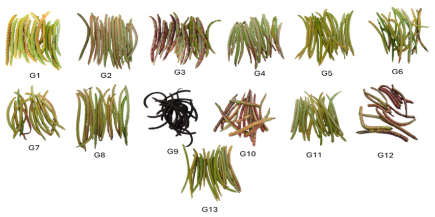
Figure 3.
Representative digital images of green beans from 13 cowpea genotypes, illustrating phenotypic variability in size, shape, color, and seed coat characteristics. G1 - BRS Exuberante, G2 - BRS Miranda, G3 - BRS Novaera, G4 - BRS Olhonegro, G5 - BRS Pajeú, G6 - Paulistinha, G7 - BRS Pingo de Ouro, G8 - BRS Tapaihum, G9 - BRS Verdejante, G10 - Corujinha, G11 - IPA 206, G12 - Rabo de tatu, G13 - Sempre Verde.
Figure 3.
Representative digital images of green beans from 13 cowpea genotypes, illustrating phenotypic variability in size, shape, color, and seed coat characteristics. G1 - BRS Exuberante, G2 - BRS Miranda, G3 - BRS Novaera, G4 - BRS Olhonegro, G5 - BRS Pajeú, G6 - Paulistinha, G7 - BRS Pingo de Ouro, G8 - BRS Tapaihum, G9 - BRS Verdejante, G10 - Corujinha, G11 - IPA 206, G12 - Rabo de tatu, G13 - Sempre Verde.
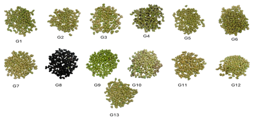

Table 1.
Comparative performance analysis of machine learning algorithms for cowpea pod classification using different embedding architectures.
Table 1.
Comparative performance analysis of machine learning algorithms for cowpea pod classification using different embedding architectures.
| Model | Performance of Classification Models | |||||||||
| Embedder InceptionV3 | ||||||||||
|
Train Time (s) |
Test Time (s) |
AUC | CA | F1 | Precision | Recall | MCC | Specificity | LogLoss | |
| Neural Network | 19.282 | 6.472 | 1.000 | 1.000 | 1.000 | 1.000 | 1.000 | 1.000 | 1.000 | 0.001 |
| SVM | 10.295 | 6.421 | 1.000 | 1.000 | 1.000 | 1.000 | 1.000 | 1.000 | 1.000 | 0.403 |
| kNN | 4.649 | 2.623 | 0.998 | 0.942 | 0.943 | 0.946 | 0.942 | 0.938 | 0.995 | 0.236 |
| Gradient Boosting | 1422.669 | 3.291 | 0.987 | 0.896 | 0.896 | 0.901 | 0.896 | 0.888 | 0.991 | 0.631 |
| Random Forest | 5.395 | 2.920 | 0.998 | 0.969 | 0.970 | 0.972 | 0.969 | 0.967 | 0.997 | 0.596 |
| Tree | 15.875 | 0.001 | 0.878 | 0.750 | 0.749 | 0.752 | 0.750 | 0.730 | 0.979 | 8.076 |
| Embedder SqueezeNet | ||||||||||
| Neural Network | 10.858 | 3.479 | 1.000 | 1.000 | 1.000 | 1.000 | 1.000 | 1.000 | 1.000 | 0.008 |
| SVM | 5.693 | 3.611 | 1.000 | 0.992 | 0.992 | 0.992 | 0.992 | 0.992 | 0.999 | 0.394 |
| kNN | 2.269 | 1.680 | 0.998 | 0.958 | 0.958 | 0.959 | 0.958 | 0.954 | 0.996 | 0.291 |
| Gradient Boosting | 830.300 | 1.683 | 0.996 | 0.923 | 0.923 | 0.927 | 0.923 | 0.917 | 0.994 | 0.353 |
| Random Forest | 3.206 | 1.382 | 0.999 | 0.965 | 0.965 | 0.967 | 0.965 | 0.963 | 0.997 | 0.449 |
| Tree | 9.370 | 0.001 | 0.872 | 0.746 | 0.745 | 0.752 | 0.746 | 0.726 | 0.979 | 8.484 |
| Embedder VGG16 | ||||||||||
| Neural Network | 36.035 | 12.437 | 1.000 | 1.000 | 1.000 | 1.000 | 1.000 | 1.000 | 1.000 | 0.001 |
| SVM | 14.491 | 12.647 | 0.999 | 0.962 | 0.963 | 0.971 | 0.962 | 0.959 | 0.997 | 0.461 |
| kNN | 8.466 | 6.746 | 0.997 | 0.954 | 0.955 | 0.957 | 0.954 | 0.950 | 0.996 | 0.257 |
| Gradient Boosting | 1364.514 | 5.738 | 0.999 | 0.954 | 0.954 | 0.956 | 0.954 | 0.950 | 0.996 | 0.187 |
| Random Forest | 8.704 | 5.760 | 1.000 | 0.992 | 0.992 | 0.992 | 0.992 | 0.992 | 0.999 | 0.354 |
| Tree | 22.816 | 0.004 | 0.916 | 0.831 | 0.831 | 0.839 | 0.831 | 0.817 | 0.986 | 5.575 |
| Embedder VGG19 | ||||||||||
| Neural Network | 40.057 | 15.503 | 1.000 | 1.000 | 1.000 | 1.000 | 1.000 | 1.000 | 1.000 | 0.000 |
| SVM | 24.156 | 15.626 | 1.000 | 0.981 | 0.981 | 0.985 | 0.981 | 0.979 | 0.998 | 0.440 |
| kNN | 9.128 | 7.876 | 0.998 | 0.946 | 0.946 | 0.949 | 0.946 | 0.942 | 0.996 | 0.217 |
| Gradient Boosting | 1727.015 | 7.107 | 0.997 | 0.946 | 0.947 | 0.951 | 0.946 | 0.942 | 0.996 | 0.311 |
| Random Forest | 9.988 | 6.919 | 0.999 | 0.988 | 0.988 | 0.989 | 0.988 | 0.988 | 0.999 | 0.381 |
| Tree | 28.002 | 0.001 | 0.906 | 0.819 | 0.819 | 0.827 | 0.819 | 0.805 | 0.985 | 6.249 |
Table 2.
Confusion matrix for classifying green cowpea pods using a Neural Network and the InceptionV3 extractor.
Table 2.
Confusion matrix for classifying green cowpea pods using a Neural Network and the InceptionV3 extractor.
| Classification Matrix and Predicted Errors | ||||||||||||||
| Genotypes | G1 | G2 | G3 | G4 | G5 | G6 | G7 | G8 | G9 | G10 | G11 | G12 | G13 | ∑ |
| G1 | 20.0 | 0.0 | 0.0 | 0.0 | 0.0 | 0.0 | 0.0 | 0.0 | 0.0 | 0.0 | 0.0 | 0.0 | 0.0 | 20 |
| G2 | 0.0 | 20.0 | 0.0 | 0.0 | 0.0 | 0.0 | 0.0 | 0.0 | 0.0 | 0.0 | 0.0 | 0.0 | 0.0 | 20 |
| G3 | 0.0 | 0.0 | 20.0 | 0.0 | 0.0 | 0.0 | 0.0 | 0.0 | 0.0 | 0.0 | 0.0 | 0.0 | 0.0 | 20 |
| G4 | 0.0 | 0.0 | 0.0 | 20.0 | 0.0 | 0.0 | 0.0 | 0.0 | 0.0 | 0.0 | 0.0 | 0.0 | 0.0 | 20 |
| G5 | 0.0 | 0.0 | 0.0 | 0.0 | 19.9 | 0.0 | 0.0 | 0.0 | 0.0 | 0.0 | 0.0 | 0.0 | 0.0 | 20 |
| G6 | 0.0 | 0.0 | 0.0 | 0.0 | 0.0 | 20.0 | 0.0 | 0.0 | 0.0 | 0.0 | 0.0 | 0.0 | 0.0 | 20 |
| G7 | 0.0 | 0.0 | 0.0 | 0.0 | 0.0 | 0.0 | 20.0 | 0.0 | 0.0 | 0.0 | 0.0 | 0.0 | 0.0 | 20 |
| G8 | 0.0 | 0.0 | 0.0 | 0.0 | 0.0 | 0.0 | 0.0 | 20.0 | 0.0 | 0.0 | 0.0 | 0.0 | 0.0 | 20 |
| G9 | 0.0 | 0.0 | 0.0 | 0.0 | 0.0 | 0.0 | 0.0 | 0.0 | 20.0 | 0.0 | 0.0 | 0.0 | 0.0 | 20 |
| G10 | 0.0 | 0.0 | 0.0 | 0.0 | 0.0 | 0.0 | 0.0 | 0.0 | 0.0 | 20.0 | 0.0 | 0.0 | 0.0 | 20 |
| G11 | 0.0 | 0.0 | 0.0 | 0.0 | 0.0 | 0.0 | 0.0 | 0.0 | 0.0 | 0.0 | 20.0 | 0.0 | 0.0 | 20 |
| G12 | 0.0 | 0.0 | 0.0 | 0.0 | 0.0 | 0.0 | 0.0 | 0.0 | 0.0 | 0.0 | 0.0 | 20.0 | 0.0 | 20 |
| G13 | 0.0 | 0.0 | 0.0 | 0.0 | 0.0 | 0.0 | 0.0 | 0.0 | 0.0 | 0.0 | 0.0 | 0.0 | 19.9 | 20 |
| ∑ | 20 | 20 | 20 | 20 | 20 | 20 | 20 | 20 | 20 | 20 | 20 | 20 | 20 | 260 |
G1 - BRS Exuberante, G2 - BRS Miranda, G3 - BRS Novaera, G4 - BRS Olhonegro, G5 - BRS Pajeú, G6 - Paulistinha, G7 - BRS Pingo de Ouro, G8 - BRS Tapaihum, G9 - BRS Verdejante, G10 - Corujinha, G11 - IPA 206, G12 - Rabo de tatu, G13 - Sempre Verde.
Table 3.
Evaluation of the performance of a Neural Network under different configurations of activation functions and optimization algorithms for the classification of green cowpea pods.
Table 3.
Evaluation of the performance of a Neural Network under different configurations of activation functions and optimization algorithms for the classification of green cowpea pods.
| Performance metrics | ||||||||||
| Activation function | Solver L-BFGS-B | |||||||||
| Train time (s) | Test time (S) | AUC | CA | F1 | Prec | Recall | MCC | Specifity | LogLoss | |
| Identity | 16.827 | 5.936 | 1.000 | 1.000 | 1.000 | 1.000 | 1.000 | 1.000 | 1.000 | 0.003 |
| Logistic | 24.234 | 7.592 | 1.000 | 1.000 | 1.000 | 1.000 | 1.000 | 1.000 | 1.000 | 0.002 |
| Tan Hyperbolic | 16.387 | 5.555 | 1.000 | 1.000 | 1.000 | 1.000 | 1.000 | 1.000 | 1.000 | 0.002 |
| ReLu | 16.028 | 6.528 | 1.000 | 1.000 | 1.000 | 1.000 | 1.000 | 1.000 | 1.000 | 0.001 |
| Solver SGD | ||||||||||
| Identity | 27.659 | 6.025 | 1.000 | 0.996 | 0.996 | 0.996 | 0.996 | 0.996 | 1.000 | 0.025 |
| Logistic | 68.693 | 6.582 | 1.000 | 0.996 | 0.996 | 0.996 | 0.996 | 0.996 | 1.000 | 0.647 |
| Tan Hyperbolic | 73.822 | 7.031 | 1.000 | 1.000 | 1.000 | 1.000 | 1.000 | 1.000 | 1.000 | 0.049 |
| ReLu | 63.737 | 6.816 | 1.000 | 1.000 | 1.000 | 1.000 | 1.000 | 1.000 | 1.000 | 0.035 |
| Solver Adam | ||||||||||
| Identity | 21.191 | 7.094 | 1.000 | 1.000 | 1.000 | 1.000 | 1.000 | 1.000 | 1.000 | 0.004 |
| Logistic | 92.801 | 7.176 | 1.000 | 1.000 | 1.000 | 1.000 | 1.000 | 1.000 | 1.000 | 0.013 |
| Tan Hyperbolic | 25.924 | 6.346 | 1.000 | 1.000 | 1.000 | 1.000 | 1.000 | 1.000 | 1.000 | 0.006 |
| ReLu | 19.741 | 6.760 | 1.000 | 1.000 | 1.000 | 1.000 | 1.000 | 1.000 | 1.000 | 0.001 |
Table 4.
Confusion matrix of the optimized Neural Network (ReLU + L-BFGS-B) in the classification of green cowpea pod genotypes.
Table 4.
Confusion matrix of the optimized Neural Network (ReLU + L-BFGS-B) in the classification of green cowpea pod genotypes.
| Predicted Class | ||||||||||||||
| Genotypes | G1 | G2 | G3 | G4 | G5 | G6 | G7 | G8 | G9 | G10 | G11 | G12 | G13 | ∑ |
| G1 | 20.0 | 0.0 | 0.0 | 0.0 | 0.0 | 0.0 | 0.0 | 0.0 | 0.0 | 0.0 | 0.0 | 0.0 | 0.0 | 20 |
| G2 | 0.0 | 20.0 | 0.0 | 0.0 | 0.0 | 0.0 | 0.0 | 0.0 | 0.0 | 0.0 | 0.0 | 0.0 | 0.0 | 20 |
| G3 | 0.0 | 0.0 | 20.0 | 0.0 | 0.0 | 0.0 | 0.0 | 0.0 | 0.0 | 0.0 | 0.0 | 0.0 | 0.0 | 20 |
| G4 | 0.0 | 0.0 | 0.0 | 20.0 | 0.0 | 0.0 | 0.0 | 0.0 | 0.0 | 0.0 | 0.0 | 0.0 | 0.0 | 20 |
| G5 | 0.0 | 0.0 | 0.0 | 0.0 | 19.9 | 0.0 | 0.0 | 0.0 | 0.0 | 0.0 | 0.0 | 0.0 | 0.0 | 20 |
| G6 | 0.0 | 0.0 | 0.0 | 0.0 | 0.0 | 20.0 | 0.0 | 0.0 | 0.0 | 0.0 | 0.0 | 0.0 | 0.0 | 20 |
| G7 | 0.0 | 0.0 | 0.0 | 0.0 | 0.0 | 0.0 | 20.0 | 0.0 | 0.0 | 0.0 | 0.0 | 0.0 | 0.0 | 20 |
| G8 | 0.0 | 0.0 | 0.0 | 0.0 | 0.0 | 0.0 | 0.0 | 20.0 | 0.0 | 0.0 | 0.0 | 0.0 | 0.0 | 20 |
| G9 | 0.0 | 0.0 | 0.0 | 0.0 | 0.0 | 0.0 | 0.0 | 0.0 | 20.0 | 0.0 | 0.0 | 0.0 | 0.0 | 20 |
| G10 | 0.0 | 0.0 | 0.0 | 0.0 | 0.0 | 0.0 | 0.0 | 0.0 | 0.0 | 20.0 | 0.0 | 0.0 | 0.0 | 20 |
| G11 | 0.0 | 0.0 | 0.0 | 0.0 | 0.0 | 0.0 | 0.0 | 0.0 | 0.0 | 0.0 | 20.0 | 0.0 | 0.0 | 20 |
| G12 | 0.0 | 0.0 | 0.0 | 0.0 | 0.0 | 0.0 | 0.0 | 0.0 | 0.0 | 0.0 | 0.0 | 20.0 | 0.0 | 20 |
| G13 | 0.0 | 0.0 | 0.0 | 0.0 | 0.0 | 0.0 | 0.0 | 0.0 | 0.0 | 0.0 | 0.0 | 0.0 | 19.9 | 20 |
| ∑ | 20 | 20 | 20 | 20 | 20 | 20 | 20 | 20 | 20 | 20 | 20 | 20 | 20 | 260 |
G1 - BRS Exuberante, G2 - BRS Miranda, G3 - BRS Novaera, G4 - BRS Olhonegro, G5 - BRS Pajeú, G6 - Paulistinha, G7 - BRS Pingo de Ouro, G8 - BRS Tapaihum, G9 - BRS Verdejante, G10 - Corujinha, G11 - IPA 206, G12 - Rabo de tatu, G13 - Sempre Verde.
Table 5.
Comparative performance of SVM and v-SVM models under different kernel functions for identifying green pods of Cowpea genotypes.
Table 5.
Comparative performance of SVM and v-SVM models under different kernel functions for identifying green pods of Cowpea genotypes.
| Performance Statistics of SVM and v-SVM Models | ||||||||||
| Kernel | Model Variant | |||||||||
| SVM | ||||||||||
| Train Time (s) | Test time (s) | AUC | CA | F1 | Prec | Recall | MCC | Specifity | LogLoss | |
| Linear | 10.536 | 6.174 | 1.000 | 1.000 | 1.000 | 1.000 | 1.000 | 1.000 | 1.000 | 0.358 |
| Polinomial | 13.542 | 8.222 | 1.000 | 1.000 | 1.000 | 1.000 | 1.000 | 1.000 | 1.000 | 0.372 |
| RBF | 13.557 | 7.855 | 1.000 | 1.000 | 1.000 | 1.000 | 1.000 | 1.000 | 1.000 | 0.398 |
| Sigmoide | 12.977 | 8.517 | 0.995 | 0.919 | 0.917 | 0.927 | 0.919 | 0.914 | 0.993 | 0.682 |
| v-SVM | ||||||||||
| Linear | 12.911 | 8.335 | 1.000 | 1.000 | 1.000 | 1.000 | 1.000 | 1.000 | 1.000 | 0.361 |
| Polinomial | 13.482 | 7.935 | 1.000 | 1.000 | 1.000 | 1.000 | 1.000 | 1.000 | 1.000 | 0.356 |
| RBF | 14.036 | 8.759 | 1.000 | 1.000 | 1.000 | 1.000 | 1.000 | 1.000 | 1.000 | 0.393 |
| Sigmoide | 13.087 | 8.365 | 1.000 | 0.988 | 0.988 | 0.989 | 0.988 | 0.988 | 0.999 | 0.414 |
Table 6.
Confusion matrix for Cowpea Genotype classification using SVM.
| Predicted Class | ||||||||||||||
| Genotypes | G1 | G2 | G3 | G4 | G5 | G6 | G7 | G8 | G9 | G10 | G11 | G12 | G13 | ∑ |
| G1 | 14.5 | 0.7 | 0.2 | 0.6 | 0.6 | 0.2 | 0.3 | 1.1 | 0.1 | 0.1 | 0.6 | 0.1 | 0.8 | 20 |
| G2 | 0.6 | 13.6 | 0.6 | 0.7 | 0.9 | 0.5 | 0.4 | 0.9 | 0.1 | 0.2 | 0.5 | 0.2 | 0.8 | 20 |
| G3 | 0.2 | 0.6 | 14.2 | 0.6 | 0.6 | 1.0 | 0.6 | 0.5 | 0.1 | 0.2 | 0.4 | 0.2 | 0.8 | 20 |
| G4 | 0.4 | 0.6 | 0.6 | 14.0 | 0.6 | 0.5 | 0.5 | 0.9 | 0.1 | 0.2 | 0.7 | 0.1 | 0.8 | 20 |
| G5 | 0.3 | 0.7 | 0.6 | 0.5 | 13.9 | 0.6 | 0.4 | 0.7 | 0.1 | 0.2 | 0.7 | 0.1 | 1.2 | 20 |
| G6 | 0.2 | 0.5 | 1.1 | 0.6 | 0.8 | 14.1 | 0.4 | 0.4 | 0.1 | 0.3 | 0.5 | 0.2 | 0.8 | 20 |
| G7 | 0.3 | 0.5 | 1.0 | 0.9 | 0.5 | 0.8 | 14.2 | 0.7 | 0.1 | 0.2 | 0.3 | 0.2 | 0.3 | 20 |
| G8 | 1.0 | 0.7 | 0.4 | 0.8 | 0.7 | 0.4 | 0.4 | 13.8 | 0.1 | 0.2 | 0.7 | 0.2 | 0.6 | 20 |
| G9 | 0.2 | 0.9 | 0.6 | 0.2 | 0.2 | 0.4 | 0.7 | 0.3 | 15.1 | 0.3 | 0.1 | 0.8 | 0.1 | 20 |
| G10 | 0.2 | 0.7 | 0.5 | 0.3 | 0.5 | 1.1 | 0.2 | 0.5 | 0.1 | 14.5 | 0.5 | 0.6 | 0.3 | 20 |
| G11 | 0.5 | 0.5 | 0.3 | 0.8 | 0.9 | 0.4 | 0.3 | 0.9 | 0.1 | 0.2 | 14.0 | 0.1 | 1.0 | 20 |
| G12 | 0.2 | 0.5 | 0.8 | 0.2 | 0.3 | 0.5 | 0.3 | 0.6 | 0.2 | 1.0 | 0.1 | 15.0 | 0.3 | 20 |
| G13 | 0.6 | 0.5 | 0.6 | 0.6 | 1.3 | 0.5 | 0.2 | 0.7 | 0.1 | 0.2 | 0.7 | 0.1 | 13.9 | 20 |
| ∑ | 19 | 21 | 21 | 21 | 22 | 21 | 19 | 22 | 17 | 18 | 20 | 18 | 22 | 260 |
G1 - BRS Exuberante, G2 - BRS Miranda, G3 - BRS Novaera, G4 - BRS Olhonegro, G5 - BRS Pajeú, G6 - Paulistinha, G7 - BRS Pingo de Ouro, G8 - BRS Tapaihum, G9 - BRS Verdejante, G10 - Corujinha, G11 - IPA 206, G12 - Rabo de tatu, G13 - Sempre Verde.
Table 7.
Performance Metrics of the Artificial Neural Network during validation.
| Performance Metrics | ||||||||
| Model Architecture |
||||||||
| Train time (s) | Test time (s) | AUC | CA | F1 | Prec | Recall | MCC | |
| Neural Network | N/A | N/A | 1.000 | 1.000 | 1.000 | 1.000 | 1.000 | 1.000 |
N/A = Information not provided by the program due to very short processing time.
Table 8.
Performance Metrics of the SVM during validation.
| Performance Metrics | ||||||||
| Model Architecture |
||||||||
| Train time (s) | Test time (s) | AUC | CA | F1 | Prec | Recall | MCC | |
| SVM | N/A | N/A | 1.000 | 1.000 | 1.000 | 1.000 | 1.000 | 1.000 |
N/A = Information not provided by the program due to very short processing time.
Table 9.
Confusion Matrix of the Artificial Neural Network performance in the validation phase.
| Predicted Class | ||||||||||||||
| G1 | G2 | G3 | G4 | G5 | G6 | G7 | G8 | G9 | G10 | G11 | G12 | G13 | ∑ | |
| G1 | 5.0 | 0.0 | 0.0 | 0.0 | 0.0 | 0.0 | 0.0 | 0.0 | 0.0 | 0.0 | 0.0 | 0.0 | 0.0 | 5 |
| G2 | 0.0 | 5.0 | 0.0 | 0.0 | 0.0 | 0.0 | 0.0 | 0.0 | 0.0 | 0.0 | 0.0 | 0.0 | 0.0 | 5 |
| G3 | 0.0 | 0.0 | 5.0 | 0.0 | 0.0 | 0.0 | 0.0 | 0.0 | 0.0 | 0.0 | 0.0 | 0.0 | 0.0 | 5 |
| G4 | 0.0 | 0.0 | 0.0 | 5.0 | 0.0 | 0.0 | 0.0 | 0.0 | 0.0 | 0.0 | 0.0 | 0.0 | 0.0 | 5 |
| G5 | 0.0 | 0.0 | 0.0 | 0.0 | 5.0 | 0.0 | 0.0 | 0.0 | 0.0 | 0.0 | 0.0 | 0.0 | 0.0 | 5 |
| G6 | 0.0 | 0.0 | 0.0 | 0.0 | 0.0 | 5.0 | 0.0 | 0.0 | 0.0 | 0.0 | 0.0 | 0.0 | 0.0 | 5 |
| G7 | 0.0 | 0.0 | 0.0 | 0.0 | 0.0 | 0.0 | 5.0 | 0.0 | 0.0 | 0.0 | 0.0 | 0.0 | 0.0 | 5 |
| G8 | 0.0 | 0.0 | 0.0 | 0.0 | 0.0 | 0.0 | 0.0 | 5.0 | 0.0 | 0.0 | 0.0 | 0.0 | 0.0 | 5 |
| G9 | 0.0 | 0.0 | 0.0 | 0.0 | 0.0 | 0.0 | 0.0 | 0.0 | 5.0 | 0.0 | 0.0 | 0.0 | 0.0 | 5 |
| G10 | 0.0 | 0.0 | 0.0 | 0.0 | 0.0 | 0.0 | 0.0 | 0.0 | 0.0 | 5.0 | 0.0 | 0.0 | 0.0 | 5 |
| G11 | 0.0 | 0.0 | 0.0 | 0.0 | 0.0 | 0.0 | 0.0 | 0.0 | 0.0 | 0.0 | 5.0 | 0.0 | 0.0 | 5 |
| G12 | 0.0 | 0.0 | 0.0 | 0.0 | 0.0 | 0.0 | 0.0 | 0.0 | 0.0 | 0.0 | 0.0 | 5.0 | 0.0 | 5 |
| G13 | 0.0 | 0.0 | 0.0 | 0.0 | 0.0 | 0.0 | 0.0 | 0.0 | 0.0 | 0.0 | 0.0 | 0.0 | 5.0 | 5 |
| ∑ | 5 | 5 | 5 | 5 | 5 | 5 | 5 | 5 | 5 | 5 | 5 | 5 | 5 | 65 |
G1 - BRS Exuberante, G2 - BRS Miranda, G3 - BRS Novaera, G4 - BRS Olhonegro, G5 - BRS Pajeú, G6 - Paulistinha, G7 - BRS Pingo de Ouro, G8 - BRS Tapaihum, G9 - BRS Verdejante, G10 - Corujinha, G11 - IPA 206, G12 - Rabo de tatu, G13 - Sempre Verde.
Table 10.
Confusion Matrix of the SVM performance in the validation phase.
| Predicted Class | ||||||||||||||
| Genotypes | G1 | G2 | G3 | G4 | G5 | G6 | G7 | G8 | G9 | G10 | G11 | G12 | G13 | ∑ |
| G1 | 3.7 | 0.1 | 0.1 | 0.1 | 0.1 | 0.0 | 0.1 | 0.3 | 0.0 | 0.0 | 0.2 | 0.0 | 0.2 | 5 |
| G2 | 0.1 | 3.7 | 0.1 | 0.1 | 0.2 | 0.1 | 0.1 | 0.2 | 0.0 | 0.0 | 0.1 | 0.0 | 0.1 | 5 |
| G3 | 0.0 | 0.1 | 3.9 | 0.1 | 0.1 | 0.2 | 0.1 | 0.1 | 0.0 | 0.0 | 0.1 | 0.0 | 0.1 | 5 |
| G4 | 0.1 | 0.1 | 0.1 | 3.6 | 0.1 | 0.1 | 0.1 | 0.2 | 0.0 | 0.0 | 0.2 | 0.0 | 0.2 | 5 |
| G5 | 0.1 | 0.2 | 0.1 | 0.1 | 3.6 | 0.1 | 0.1 | 0.2 | 0.0 | 0.0 | 0.1 | 0.0 | 0.2 | 5 |
| G6 | 0.0 | 0.1 | 0.2 | 0.1 | 0.1 | 3.9 | 0.1 | 0.1 | 0.0 | 0.1 | 0.1 | 0.0 | 0.1 | 5 |
| G7 | 0.1 | 0.1 | 0.2 | 0.2 | 0.1 | 0.2 | 3.7 | 0.2 | 0.0 | 0.0 | 0.1 | 0.1 | 0.1 | 5 |
| G8 | 0.2 | 0.2 | 0.1 | 0.2 | 0.1 | 0.1 | 0.1 | 3.6 | 0.0 | 0.0 | 0.2 | 0.0 | 0.2 | 5 |
| G9 | 0.0 | 0.2 | 0.1 | 0.0 | 0.0 | 0.1 | 0.2 | 0.1 | 3.9 | 0.1 | 0.0 | 0.2 | 0.0 | 5 |
| G10 | 0.0 | 0.2 | 0.1 | 0.1 | 0.1 | 0.3 | 0.1 | 0.1 | 0.0 | 3.7 | 0.1 | 0.1 | 0.1 | 5 |
| G11 | 0.1 | 0.1 | 0.1 | 0.2 | 0.2 | 0.1 | 0.0 | 0.2 | 0.0 | 0.0 | 3.8 | 0.0 | 0.2 | 5 |
| G12 | 0.0 | 0.1 | 0.2 | 0.0 | 0.1 | 0.1 | 0.1 | 0.2 | 0.1 | 0.2 | 0.0 | 3.8 | 0.1 | 5 |
| G13 | 0.2 | 0.1 | 0.1 | 0.1 | 0.3 | 0.1 | 0.0 | 0.2 | 0.0 | 0.0 | 0.2 | 0.0 | 3.5 | 5 |
| ∑ | 5 | 5 | 5 | 5 | 5 | 5 | 5 | 6 | 4 | 4 | 5 | 5 | 5 | 65 |
G1 - BRS Exuberante, G2 - BRS Miranda, G3 - BRS Novaera, G4 - BRS Olhonegro, G5 - BRS Pajeú, G6 - Paulistinha, G7 - BRS Pingo de Ouro, G8 - BRS Tapaihum, G9 - BRS Verdejante, G10 - Corujinha, G11 - IPA 206, G12 - Rabo de tatu, G13 - Sempre Verde.
Table 11.
Performance Comparison of Machine Learning Models for Green Bean Classification Using InceptionV3.
Table 11.
Performance Comparison of Machine Learning Models for Green Bean Classification Using InceptionV3.
| M. | Performance Metrics | |||||||||
| Embedder InceptionV3 | ||||||||||
| Train time (s) | Test time (s) | AUC | CA | F1 | Precision | Recall | MCC | Specificity | LogLoss | |
| Neural Network | 18.389 | 6.774 | 1.000 | 0.977 | 0.977 | 0.978 | 0.977 | 0.975 | 0.998 | 0.075 |
| SVM | 10.936 | 7.170 | 1.000 | 0.977 | 0.977 | 0.977 | 0.977 | 0.975 | 0.998 | 0.413 |
| kNN | 4.462 | 3.385 | 0.987 | 0.892 | 0.890 | 0.904 | 0.892 | 0.885 | 0.991 | 0.669 |
| Gradient Boosting | 1881.558 | 4.043 | 0.960 | 0.796 | 0.799 | 0.809 | 0.796 | 0.780 | 0.983 | 1.336 |
| Random Forest | 5.596 | 3.416 | 0.970 | 0.804 | 0.802 | 0.808 | 0.804 | 0.788 | 0.984 | 1.168 |
| Tree | 22.471 | 0.002 | 0.839 | 0.681 | 0.684 | 0.700 | 0.681 | 0.655 | 0.973 | 10.586 |
| Embedder SqueezeNet | ||||||||||
| Neural Network | 11.292 | 3.862 | 0.998 | 0.962 | 0.961 | 0.965 | 0.962 | 0.959 | 0.997 | 0.204 |
| SVM | 6.629 | 4.516 | 0.995 | 0.962 | 0.962 | 0.964 | 0.962 | 0.959 | 0.997 | 0.497 |
| kNN | 3.085 | 4.539 | 0.987 | 0.865 | 0.860 | 0.868 | 0.865 | 0.855 | 0.989 | 0.662 |
| Gradient Boosting | 973.617 | 2.123 | 0.980 | 0.812 | 0.816 | 0.829 | 0.812 | 0.797 | 0.984 | 0.855 |
| Random Forest | 4.301 | 2.154 | 0.981 | 0.865 | 0.865 | 0.867 | 0.865 | 0.854 | 0.989 | 0.858 |
| Tree | 14.063 | 0.018 | 0.796 | 0.581 | 0.585 | 0.596 | 0.581 | 0.546 | 0.965 | 13.79 |
| Embedder VGG16 | ||||||||||
| Neural Network | 12.326 | 2.451 | 0.998 | 0.962 | 0.961 | 0.965 | 0.962 | 0.959 | 0.997 | 0.204 |
| SVM | 3.797 | 4.839 | 0.995 | 0.962 | 0.962 | 0.964 | 0.962 | 0.959 | 0.997 | 0.493 |
| kNN | 1.746 | 1.246 | 0.987 | 0.865 | 0.860 | 0.868 | 0.865 | 0.855 | 0.989 | 0.662 |
| Gradient Boosting | 786.044 | 1.491 | 0.980 | 0.812 | 0.816 | 0.829 | 0.812 | 0.797 | 0.984 | 0.855 |
| Random Forest | 2.228 | 1.165 | 0.980 | 0.842 | 0.837 | 0.840 | 0.842 | 0.830 | 0.987 | 0.881 |
| Tree | 9.380 | 0.001 | 0.796 | 0.581 | 0.585 | 0.596 | 0.581 | 0.546 | 0.965 | 13.379 |
| Embedder VGG19 | ||||||||||
| Neural Network | 41.144 | 12.357 | 0.978 | 0.977 | 0.977 | 0.979 | 0.977 | 0.975 | 0.998 | 0.122 |
| SVM | 18.936 | 13.163 | 0.996 | 0.985 | 0.985 | 0.985 | 0.985 | 0.983 | 0.999 | 0.436 |
| kNN | 8.464 | 6.510 | 0.979 | 0.792 | 0.788 | 0.802 | 0.792 | 0.777 | 0.983 | 0.998 |
| Gradient Boosting | 1628.294 | 6.111 | 0.980 | 0.869 | 0.871 | 0.883 | 0.869 | 0.859 | 0.989 | 0.920 |
| Random Forest | 9.468 | 5.999 | 0.984 | 0.881 | 0.881 | 0.885 | 0.881 | 0.871 | 0.990 | 0.795 |
| Tree | 30.966 | 0.000 | 0.837 | 0.681 | 0.681 | 0.688 | 0.681 | 0.655 | 0.973 | 10.714 |
Table 12.
Confusion Matrix of the Artificial Neural Network classifier for green Cowpea grain images (InceptionV3).
Table 12.
Confusion Matrix of the Artificial Neural Network classifier for green Cowpea grain images (InceptionV3).
| Predicted Class | ||||||||||||||
| Genotypes | G1 | G2 | G3 | G4 | G5 | G6 | G7 | G8 | G9 | G10 | G11 | G12 | G13 | ∑ |
| G1 | 19.1 | 0.0 | 0.0 | 0.0 | 0.0 | 0.0 | 0.8 | 0.0 | 0.0 | 0.0 | 0.0 | 0.1 | 0.0 | 20 |
| G2 | 0.0 | 19.9 | 0.0 | 0.0 | 0.0 | 0.0 | 0.0 | 0.0 | 0.0 | 0.0 | 0.0 | 0.0 | 0.0 | 20 |
| G3 | 0.0 | 0.9 | 18.9 | 0.0 | 0.0 | 0.0 | 0.1 | 0.0 | 0.0 | 0.0 | 0.0 | 0.0 | 0.1 | 20 |
| G4 | 0.0 | 0.0 | 0.0 | 19.7 | 0.0 | 0.3 | 0.0 | 0.0 | 0.0 | 0.0 | 0.0 | 0.0 | 0.0 | 20 |
| G5 | 0.0 | 0.0 | 0.0 | 0.0 | 18.3 | 0.2 | 1.3 | 0.0 | 0.0 | 0.0 | 0.1 | 0.0 | 0.0 | 20 |
| G6 | 0.4 | 0.1 | 0.0 | 0.0 | 1.9 | 17.5 | 0.1 | 0.0 | 0.0 | 0.0 | 0.0 | 0.0 | 0.0 | 20 |
| G7 | 0.0 | 0.0 | 0.0 | 0.1 | 0.2 | 0.0 | 19.4 | 0.0 | 0.0 | 0.0 | 0.1 | 0.0 | 0.1 | 20 |
| G8 | 0.0 | 0.0 | 0.0 | 0.0 | 0.0 | 0.0 | 0.0 | 20.0 | 0.0 | 0.0 | 0.0 | 0.0 | 0.0 | 20 |
| G9 | 0.0 | 0.0 | 0.0 | 0.0 | 0.0 | 0.0 | 0.0 | 0.0 | 20.0 | 0.0 | 0.0 | 0.0 | 0.0 | 20 |
| G10 | 0.0 | 0.0 | 0.0 | 0.0 | 0.0 | 0.0 | 0.0 | 0.0 | 0.0 | 20.0 | 0.0 | 0.0 | 0.0 | 20 |
| G11 | 0.0 | 0.0 | 0.0 | 0.0 | 0.0 | 0.0 | 0.1 | 0.0 | 0.1 | 0.0 | 19.6 | 0.0 | 0.2 | 20 |
| G12 | 0.0 | 0.0 | 0.0 | 0.0 | 0.0 | 0.0 | 0.0 | 0.0 | 0.0 | 0.0 | 0.0 | 20.0 | 0.0 | 20 |
| G13 | 0.0 | 0.1 | 0.2 | 0.0 | 0.0 | 0.0 | 0.1 | 0.0 | 0.0 | 0.0 | 1.0 | 0.0 | 18.5 | 20 |
| ∑ | 20 | 21 | 19 | 20 | 21 | 18 | 22 | 20 | 20 | 20 | 21 | 20 | 19 | 260 |
G1 - BRS Exuberante, G2 - BRS Miranda, G3 - BRS Novaera, G4 - BRS Olhonegro, G5 - BRS Pajeú, G6 - Paulistinha, G7 - BRS Pingo de Ouro, G8 - BRS Tapaihum, G9 - BRS Verdejante, G10 - Corujinha, G11 - IPA 206, G12 - Rabo de tatu, G13 - Sempre Verde.
Table 13.
Performance Metrics of the Artificial Neural Network classifier with InceptionV3 features across different activation functions and Solvers.
Table 13.
Performance Metrics of the Artificial Neural Network classifier with InceptionV3 features across different activation functions and Solvers.
| Performance Metrics | ||||||||||
| Activation Function | Solver L-BFGS-B | |||||||||
| Train time (s) | Test time (s) | AUC | CA | F1 | Prec | Recall | MCC | Specifity | LogLoss | |
| Identity | 24.358 | 7.161 | 1.000 | 0.977 | 0.977 | 0.977 | 0.977 | 0.975 | 0.998 | 0.096 |
| Logistics | 22.966 | 7.387 | 1.000 | 0.965 | 0.965 | 0.968 | 0.965 | 0.963 | 0.997 | 0.093 |
| Tan Hyperbolic | 22.300 | 7.073 | 1.000 | 0.977 | 0.977 | 0.977 | 0.977 | 0.975 | 0.998 | 0.061 |
| ReLu | 22.727 | 7.066 | 1.000 | 0.977 | 0.977 | 0.978 | 0.977 | 0.975 | 0.998 | 0.075 |
| Solver SGD | ||||||||||
| Identity | 57.343 | 8.258 | 0.999 | 0.954 | 0.954 | 0.955 | 0.954 | 0.950 | 0.996 | 0.156 |
| Logistics | 78.067 | 7.806 | 0.994 | 0.892 | 0.892 | 0.897 | 0.892 | 0.884 | 0.991 | 0.918 |
| Tan Hyperbolic | 71.734 | 7.522 | 0.999 | 0.965 | 0.965 | 0.966 | 0.965 | 0.963 | 0.997 | 0.186 |
| ReLu | 78.120 | 7.535 | 0.999 | 0.965 | 0.965 | 0.967 | 0.965 | 0.963 | 0.997 | 0.166 |
| Solver Adam | ||||||||||
| Identity | 23.292 | 8.074 | 0.999 | 0.946 | 0.946 | 0.948 | 0.946 | 0.942 | 0.996 | 0.112 |
| Logistics | 96.284 | 7.802 | 1.000 | 0.981 | 0.981 | 0.981 | 0.981 | 0.979 | 0.998 | 0.090 |
| Tan Hyperbolic | 33.266 | 8.568 | 1.000 | 0.969 | 0.969 | 0.971 | 0.969 | 0.967 | 0.997 | 0.080 |
| ReLu | 25.016 | 7.880 | 0.999 | 0.965 | 0.965 | 0.967 | 0.965 | 0.963 | 0.997 | 0.103 |
Table 14.
Confusion Matrix for the Artificial Neural Network classifier optimized with ReLU activation and L-BFGS-B Solver.
Table 14.
Confusion Matrix for the Artificial Neural Network classifier optimized with ReLU activation and L-BFGS-B Solver.
| Predicted model | ||||||||||||||
| Genotypes | G1 | G2 | G3 | G4 | G5 | G6 | G7 | G8 | G9 | G10 | G11 | G12 | G13 | ∑ |
| G1 | 19.1 | 0.0 | 0.0 | 0.0 | 0.0 | 0.0 | 0.8 | 0.0 | 0.0 | 0.0 | 0.0 | 0.1 | 0.0 | 20 |
| G2 | 0.0 | 19.9 | 0.0 | 0.0 | 0.0 | 0.0 | 0.0 | 0.0 | 0.0 | 0.0 | 0.0 | 0.0 | 0.0 | 20 |
| G3 | 0.0 | 0.9 | 18.9 | 0.0 | 0.0 | 0.0 | 0.1 | 0.0 | 0.0 | 0.0 | 0.0 | 0.0 | 0.1 | 20 |
| G4 | 0.0 | 0.0 | 0.0 | 19.7 | 0.0 | 0.3 | 0.0 | 0.0 | 0.0 | 0.0 | 0.0 | 0.0 | 0.0 | 20 |
| G5 | 0.0 | 0.0 | 0.0 | 0.0 | 18.3 | 0.2 | 1.3 | 0.0 | 0.0 | 0.0 | 0.1 | 0.0 | 0.0 | 20 |
| G6 | 0.4 | 0.1 | 0.0 | 0.0 | 1.9 | 17.5 | 0.1 | 0.0 | 0.0 | 0.0 | 0.0 | 0.0 | 0.0 | 20 |
| G7 | 0.0 | 0.0 | 0.0 | 0.1 | 0.2 | 0.0 | 19.4 | 0.0 | 0.0 | 0.0 | 0.1 | 0.0 | 0.1 | 20 |
| G8 | 0.0 | 0.0 | 0.0 | 0.0 | 0.0 | 0.0 | 0.0 | 20.0 | 0.0 | 0.0 | 0.0 | 0.0 | 0.0 | 20 |
| G9 | 0.0 | 0.0 | 0.0 | 0.0 | 0.0 | 0.0 | 0.0 | 0.0 | 20.0 | 0.0 | 0.0 | 0.0 | 0.0 | 20 |
| G10 | 0.0 | 0.0 | 0.0 | 0.0 | 0.0 | 0.0 | 0.0 | 0.0 | 0.0 | 20.0 | 0.0 | 0.0 | 0.0 | 20 |
| G11 | 0.0 | 0.0 | 0.0 | 0.0 | 0.0 | 0.0 | 0.1 | 0.0 | 0.1 | 0.0 | 19.6 | 0.0 | 0.2 | 20 |
| G12 | 0.0 | 0.0 | 0.0 | 0.0 | 0.0 | 0.0 | 0.0 | 0.0 | 0.0 | 0.0 | 0.0 | 20.0 | 0.0 | 20 |
| G13 | 0.0 | 0.1 | 0.2 | 0.0 | 0.0 | 0.0 | 0.1 | 0.0 | 0.0 | 0.0 | 1.0 | 0.0 | 18.5 | 20 |
| ∑ | 20 | 21 | 19 | 20 | 21 | 18 | 22 | 20 | 20 | 20 | 21 | 20 | 19 | 260 |
G1 - BRS Exuberante, G2 - BRS Miranda, G3 - BRS Novaera, G4 - BRS Olhonegro, G5 - BRS Pajeú, G6 - Paulistinha, G7 - BRS Pingo de Ouro, G8 - BRS Tapaihum, G9 - BRS Verdejante, G10 - Corujinha, G11 - IPA 206, G12 - Rabo de tatu, G13 - Sempre Verde.
Table 15.
Performance Comparison of SVM and v-SVM algorithms across different kernel functions.
| Performance Metrics | ||||||||||
| Kernel | Machine Learning Models | |||||||||
| SVM | ||||||||||
| Train Time (s) |
Test Time (s) |
AUC | CA | F1 | Prec | Recall | MCC | Specifity | LogLoss | |
| Linear | 10.668 | 6.539 | 1.000 | 0.977 | 0.977 | 0.977 | 0.977 | 0.975 | 0.998 | 0.408 |
| Polynomial | 10.158 | 7.078 | 1.000 | 0.977 | 0.977 | 0.978 | 0.977 | 0.975 | 0.998 | 0.400 |
| RBF | 11.084 | 6.589 | 0.999 | 0.954 | 0.954 | 0.955 | 0.954 | 0.950 | 0.996 | 0.457 |
| Sigmoid | 10.830 | 6.096 | 0.968 | 0.769 | 0.771 | 0.794 | 0.769 | 0.752 | 0.981 | 1.035 |
| v-SVM | ||||||||||
| Linear | 10.289 | 6.754 | 0.998 | 0.942 | 0.942 | 0.947 | 0.942 | 0.938 | 0.995 | 0.501 |
| Polynomial | 10.186 | 6.863 | 1.000 | 0.950 | 0.950 | 0.957 | 0.950 | 0.946 | 0.996 | 0.454 |
| RBF | 10.706 | 7.034 | 1.000 | 0.965 | 0.965 | 0.967 | 0.965 | 0.963 | 0.997 | 0.456 |
| Sigmoid | 9.812 | 7.207 | 0.990 | 0.869 | 0.867 | 0.869 | 0.869 | 0.859 | 0.989 | 0.678 |
Table 16.
Confusion Matrix for the SVM classifier operating with a polynomial Kernel.
| Predicted model | ||||||||||||||
| Genotypes | G1 | G2 | G3 | G4 | G5 | G6 | G7 | G8 | G9 | G10 | G11 | G12 | G13 | ∑ |
| G1 | 13.7 | 0.9 | 0.8 | 0.2 | 0.8 | 0.6 | 1.0 | 0.1 | 0.3 | 0.2 | 0.4 | 0.3 | 0.6 | 20 |
| G2 | 0.6 | 12.8 | 0.9 | 0.3 | 0.9 | 0.6 | 0.9 | 0.1 | 0.4 | 0.2 | 0.9 | 0.3 | 1.1 | 20 |
| G3 | 0.7 | 0.9 | 14.1 | 0.2 | 0.4 | 0.3 | 0.8 | 0.1 | 0.3 | 0.2 | 0.6 | 0.2 | 1.2 | 20 |
| G4 | 0.5 | 0.7 | 0.3 | 15.4 | 0.5 | 0.8 | 0.2 | 0.1 | 0.3 | 0.1 | 0.4 | 0.2 | 0.3 | 20 |
| G5 | 0.6 | 0.8 | 0.4 | 0.2 | 13.4 | 1.4 | 1.0 | 0.1 | 0.3 | 0.1 | 0.7 | 0.3 | 0.7 | 20 |
| G6 | 0.6 | 0.6 | 0.3 | 0.5 | 1.9 | 14.2 | 0.5 | 0.1 | 0.2 | 0.1 | 0.4 | 0.2 | 0.4 | 20 |
| G7 | 0.7 | 0.9 | 0.7 | 0.2 | 1.0 | 0.5 | 12.8 | 0.1 | 0.4 | 0.2 | 1.0 | 0.3 | 1.3 | 20 |
| G8 | 0.5 | 0.7 | 0.6 | 0.5 | 0.4 | 0.7 | 0.3 | 14.3 | 0.5 | 0.3 | 0.5 | 0.2 | 0.6 | 20 |
| G9 | 0.5 | 0.8 | 0.5 | 0.2 | 0.6 | 0.4 | 0.6 | 0.1 | 14.0 | 0.2 | 1.1 | 0.3 | 0.9 | 20 |
| G10 | 0.4 | 0.5 | 0.8 | 0.1 | 0.3 | 0.2 | 0.6 | 0.1 | 0.7 | 14.3 | 1.0 | 0.4 | 0.6 | 20 |
| G11 | 0.4 | 0.9 | 0.5 | 0.2 | 0.7 | 0.3 | 1.0 | 0.1 | 0.6 | 0.2 | 13.7 | 0.2 | 1.0 | 20 |
| G12 | 0.5 | 1.0 | 0.4 | 0.2 | 0.6 | 0.3 | 0.7 | 0.1 | 0.4 | 0.2 | 0.6 | 14.3 | 0.7 | 20 |
| G13 | 0.4 | 1.1 | 1.1 | 0.2 | 0.8 | 0.4 | 1.0 | 0.1 | 0.4 | 0.2 | 1.2 | 0.2 | 12.8 | 20 |
| ∑ | 20 | 23 | 22 | 18 | 22 | 21 | 21 | 16 | 19 | 17 | 22 | 17 | 22 | 260 |
G1 - BRS Exuberante, G2 - BRS Miranda, G3 - BRS Novaera, G4 - BRS Olhonegro, G5 - BRS Pajeú, G6 - Paulistinha, G7 - BRS Pingo de Ouro, G8 - BRS Tapaihum, G9 - BRS Verdejante, G10 - Corujinha, G11 - IPA 206, G12 - Rabo de tatu, G13 - Sempre Verde.
Table 17.
Validation Performance Metrics for the Optimized Artificial Neural Network Model.
| Performance Metrics | ||||||||
| Model Architecture |
||||||||
| Train time (s) | Test time (s) | AUC | CA | F1 | Prec | Recall | MCC | |
| Neural Network | N/A | N/A | 1.000 | 0.923 | 0.889 | 1.000 | 0.800 | 0.917 |
N/A = Information not provided by the program due to very short processing time.
Table 18.
Confusion Matrix for the Artificial Neural Network validation process.
| Predicted model | ||||||||||||||
| Genotypes | G1 | G2 | G3 | G4 | G5 | G6 | G7 | G8 | G9 | G10 | G11 | G12 | G13 | ∑ |
| G1 | 5.0 | 0.0 | 0.0 | 0.0 | 0.0 | 0.0 | 0.0 | 0.0 | 0.0 | 0.0 | 0.0 | 0.0 | 0.0 | 5 |
| G2 | 0.0 | 4.1 | 0.2 | 0.0 | 0.0 | 0.0 | 0.0 | 0.0 | 0.0 | 0.0 | 0.0 | 0.0 | 0.7 | 5 |
| G3 | 0.0 | 0.0 | 5.0 | 0.0 | 0.0 | 0.0 | 0.0 | 0.0 | 0.0 | 0.0 | 0.0 | 0.0 | 0.0 | 5 |
| G4 | 0.0 | 0.0 | 0.0 | 5.0 | 0.0 | 0.0 | 0.0 | 0.0 | 0.0 | 0.0 | 0.0 | 0.0 | 0.0 | 5 |
| G5 | 0.0 | 0.1 | 0.0 | 0.0 | 4.4 | 0.5 | 0.0 | 0.0 | 0.0 | 0.0 | 0.0 | 0.0 | 0.0 | 5 |
| G6 | 0.0 | 0.0 | 0.0 | 0.0 | 0.0 | 5.0 | 0.0 | 0.0 | 0.0 | 0.0 | 0.0 | 0.0 | 0.0 | 5 |
| G7 | 0.0 | 0.0 | 0.1 | 0.0 | 0.0 | 0.0 | 4.0 | 0.0 | 0.0 | 0.0 | 0.9 | 0.0 | 0.0 | 5 |
| G8 | 0.0 | 0.0 | 0.0 | 0.0 | 0.0 | 0.0 | 0.0 | 5.0 | 0.0 | 0.0 | 0.0 | 0.0 | 0.0 | 5 |
| G9 | 0.0 | 0.0 | 0.0 | 0.0 | 0.0 | 0.0 | 0.0 | 0.0 | 5.0 | 0.0 | 0.0 | 0.0 | 0.0 | 5 |
| G10 | 0.0 | 0.0 | 0.0 | 0.0 | 0.0 | 0.0 | 0.0 | 0.0 | 0.0 | 5.0 | 0.0 | 0.0 | 0.0 | 5 |
| G11 | 0.0 | 0.0 | 0.0 | 0.0 | 0.0 | 0.0 | 0.5 | 0.0 | 0.0 | 0.0 | 4.4 | 0.0 | 0.0 | 5 |
| G12 | 0.0 | 0.0 | 0.0 | 0.0 | 0.0 | 0.0 | 0.0 | 0.0 | 0.0 | 0.0 | 0.0 | 5.0 | 0.0 | 5 |
| G12 | 0.0 | 0.0 | 0.0 | 0.0 | 0.0 | 0.5 | 0.0 | 0.0 | 0.0 | 0.0 | 0.0 | 0.0 | 4.4 | 5 |
| ∑ | 5 | 4 | 5 | 5 | 4 | 6 | 5 | 5 | 5 | 5 | 5 | 5 | 5 | 65 |
G1 - BRS Exuberante, G2 - BRS Miranda, G3 - BRS Novaera, G4 - BRS Olhonegro, G5 - BRS Pajeú, G6 - Paulistinha, G7 - BRS Pingo de Ouro, G8 - BRS Tapaihum, G9 - BRS Verdejante, G10 - Corujinha, G11 - IPA 206, G12 - Rabo de tatu, G13 - Sempre Verde.
Table 19.
Validation Performance Metrics for the Optimized SVM Classifier.
| Performance Metrics | ||||||||
| Model Architecture |
||||||||
| Train time (s) | Test time (s) | AUC | CA | F1 | Prec | Recall | MCC | |
| SVM | N/A | N/A | 1.000 | 0.954 | 1.000 | 1.000 | 1.000 | 0.951 |
N/A = Information not provided by the program due to very short processing time.
Table 20.
Confusion Matrix for the SVM validation process.
| Predicted model | ||||||||||||||
| Genotypes | G1 | G2 | G3 | G4 | G5 | G6 | G7 | G8 | G9 | G10 | G11 | G12 | G13 | ∑ |
| G1 | 2.9 | 0.2 | 0.2 | 0.0 | 0.3 | 0.2 | 0.4 | 0.0 | 0.1 | 0.0 | 0.1 | 0.1 | 0.4 | 5 |
| G2 | 0.1 | 3.0 | 0.2 | 0.1 | 0.3 | 0.1 | 0.1 | 0.0 | 0.1 | 0.0 | 0.2 | 0.1 | 0.6 | 5 |
| G3 | 0.2 | 0.1 | 3.8 | 0.0 | 0.1 | 0.1 | 0.1 | 0.0 | 0.1 | 0.0 | 0.2 | 0.0 | 0.2 | 5 |
| G4 | 0.3 | 0.3 | 0.1 | 3.2 | 0.2 | 0.2 | 0.1 | 0.0 | 0.1 | 0.0 | 0.2 | 0.1 | 0.1 | 5 |
| G5 | 0.1 | 0.1 | 0.1 | 0.1 | 3.7 | 0.4 | 0.2 | 0.0 | 0.0 | 0.0 | 0.1 | 0.0 | 0.1 | 5 |
| G6 | 0.1 | 0.1 | 0.1 | 0.1 | 0.1 | 4.2 | 0.1 | 0.0 | 0.0 | 0.0 | 0.1 | 0.0 | 0.1 | 5 |
| G7 | 0.2 | 0.2 | 0.2 | 0.0 | 0.2 | 0.1 | 3.0 | 0.0 | 0.1 | 0.1 | 0.6 | 0.1 | 0.1 | 5 |
| G8 | 0.1 | 0.2 | 0.1 | 0.1 | 0.1 | 0.1 | 0.1 | 3.5 | 0.1 | 0.1 | 0.2 | 0.1 | 0.2 | 5 |
| G9 | 0.1 | 0.1 | 0.1 | 0.0 | 0.1 | 0.1 | 0.1 | 0.0 | 4.0 | 0.0 | 0.1 | 0.1 | 0.2 | 5 |
| G10 | 0.1 | 0.1 | 0.1 | 0.0 | 0.1 | 0.0 | 0.1 | 0.0 | 0.2 | 3.9 | 0.2 | 0.1 | 0.1 | 5 |
| G11 | 0.1 | 0.1 | 0.2 | 0.0 | 0.2 | 0.1 | 0.4 | 0.0 | 0.2 | 0.1 | 3.3 | 0.1 | 0.2 | 5 |
| G12 | 0.1 | 0.2 | 0.1 | 0.0 | 0.1 | 0.1 | 0.1 | 0.0 | 0.1 | 0.0 | 0.1 | 3.9 | 0.1 | 5 |
| G13 | 0.1 | 0.2 | 0.1 | 0.0 | 0.2 | 0.2 | 0.2 | 0.0 | 0.1 | 0.0 | 0.2 | 0.0 | 3.6 | 5 |
| ∑ | 4 | 5 | 5 | 4 | 6 | 6 | 5 | 4 | 5 | 4 | 6 | 5 | 6 | 65 |
G1 - BRS Exuberante, G2 - BRS Miranda, G3 - BRS Novaera, G4 - BRS Olhonegro, G5 - BRS Pajeú, G6 - Paulistinha, G7 - BRS Pingo de Ouro, G8 - BRS Tapaihum, G9 - BRS Verdejante, G10 - Corujinha, G11 - IPA 206, G12 - Rabo de tatu, G13 - Sempre Verde.
Disclaimer/Publisher’s Note: The statements, opinions and data contained in all publications are solely those of the individual author(s) and contributor(s) and not of MDPI and/or the editor(s). MDPI and/or the editor(s) disclaim responsibility for any injury to people or property resulting from any ideas, methods, instructions or products referred to in the content. |
© 2026 by the authors. Licensee MDPI, Basel, Switzerland. This article is an open access article distributed under the terms and conditions of the Creative Commons Attribution (CC BY) license (http://creativecommons.org/licenses/by/4.0/).
Copyright: This open access article is published under a Creative Commons CC BY 4.0 license, which permit the free download, distribution, and reuse, provided that the author and preprint are cited in any reuse.


