

Submitted:
15 November 2026
Posted:
18 November 2026
You are already at the latest version
Abstract
The Minimum Independent Dominating Set problem asks for a smallest maximal independent set of a graph. Unless \(\mathrm{P}=\mathrm{NP}\) it is not approximable within \(n^{1-\varepsilon}\) for any \(\varepsilon>0\); it is NP-complete on cubic planar bipartite graphs and NP-hard to approximate within \(\delta B\) on bipartite graphs of maximum degree \(B\). We present version 0.0.9 of Siriaisa, an ensemble of eighteen strategies that adapts the vertex cover algorithm Salvador and the independent set algorithm Esperanza to independent domination: its exact subproblems are forests, solved by a conditioned tree dynamic program, in place of the bipartite structures of Salvador; one base strategy splits every vertex of degree larger than \(\lfloor\sqrt n\rfloor\) into unconnected copies; and the improvers include a weighted swap search. We prove that the output is an independent dominating set computed in \(O(n+m)\) expected time, with ratio at most \(\Delta\), optimal on forests, and with ratio at most \(\sqrt n\) on three classes of graphs. The degree-splitting strategy computes a dominating set of size at most \(\lfloor\sqrt n\rfloor\,(i(G)+s(G))\) on every graph, for an explicit splitting excess \(s(G)\), and the output satisfies the same bound when the decoded set is independent. The excess is at most \(n(\sqrt n+1)\), largest on complete graphs, zero for \(n\ge D^2\) on every family of bounded degree \(D\), among them the NP-hard and UG-hard bounded-degree families, and \(O(\sqrt n)\) on planar graphs; on complete multipartite, crown, wheel and double-star graphs the output is optimal. We conjecture the ratio \(O(\sqrt n)\) on all graphs; a proof would imply \(\mathrm{P}=\mathrm{NP}\). In a reduction from satisfiability, every independent dominating set of the graph of a formula with \(N\) variables and \(t\) copies of every clause, \(t\) at least the largest clause width \(W\), is a satisfying assignment, with \(N\) vertices, or has at least \(t+N\) vertices; with \(t=W\), every independent dominating set of ratio smaller than \(1+W/N\) is a satisfying assignment. This proves the \(n^{1-\varepsilon}\) inapproximability directly from satisfiability, without a gap from the PCP theorem. Through a reduction of Chlebík and Chlebíková, with an explicit edge gadget that turns a graph \(H\) into a graph \(h(H)\) with \(i(h(H))=\tau(H)+2|E(H)|\), where \(\tau(H)\) is the minimum vertex cover size, every output on \(h(H)\) decodes into a vertex cover of \(H\); we state the conditional consequences under the Unique Games Conjecture, for which a proof has been reported but not yet peer reviewed, on general graphs and, through the result of Austrin, Khot and Safra, on bounded-degree graphs. In reproducible experiments the output is optimal on 9999 of 10,000 graphs with an exact integer-program optimum, on all 95 of 112 bipartite graphs whose optimum was proved, on all 18 instances of the set cover reduction, and on 2 of the 30 instances of the vertex cover reduction with a proved optimum; on ten Khot–Regev YES instances the decoded vertex cover has ratio between 1.25 and 1.8665. We also report the results on the 68 complements of the DIMACS clique benchmark.
Keywords:
minimum independent dominating set
; minimum maximal independent set
; approximation algorithm
; forest dynamic programming
; local search
; bipartite graphs
; unique games conjecture
; P versus NP
MSC: 05C69; 68Q25; 68W25; 90C27
1. Introduction
An independent dominating set of an undirected graph is a set in which no two vertices are adjacent and every vertex of has a neighbour in D; equivalently, D is a maximal independent set. The Minimum Independent Dominating Set problem (MIDS) asks for such a set of minimum size, denoted . We write , , and for the open and closed neighbourhoods, , for the maximum degree, for the minimum vertex cover size and for the independence number. The ratio of a returned independent dominating set S is .
MIDS is among the hardest graph problems to approximate. Irving proved that, unless , no polynomial-time algorithm approximates it within any constant factor [1], and Halldórsson proved that it cannot be approximated within for any unless [2]; Damian-Iordache and Pemmaraju proved that it is NP-complete on circle graphs and, unless , not approximable within for any on circle graphs with n vertices [3]. The problem remains NP-hard on bipartite graphs: Loverov and Orlovich proved that it is NP-complete already on cubic planar bipartite graphs [4]; Manlove proved it NP-hard on cubic planar graphs [5], and Bazgan, Brankovic, Casel and Fernau derived from Manlove’s reduction that it is APX-hard on cubic graphs [6]. On graphs of maximum degree at most a constant B, every maximal independent set approximates MIDS within B, and the problem is APX-complete [7]; on cubic graphs, Alimonti and Calamoneri gave a polynomial-time algorithm with ratio , and the ratio 2 on graphs of maximum degree at most 3 [8], while Alimonti and Kann proved APX-completeness on cubic graphs of vertex cover, independent set and dominating set [9]. It is also hard to approximate on graphs of bounded degree, including bipartite ones: Chlebík and Chlebíková proved that there are absolute constants and such that for every MIDS is NP-hard to approximate within on graphs of maximum degree at most B, and that the same holds on bipartite graphs; for small degrees they obtained the NP-hard factors for , and and for bipartite graphs with and [10]. These results hold without any conjecture.
1.0.0.1. Exact algorithms and heuristics
A minimum independent dominating set can be computed in time by enumerating the maximal independent sets; Gaspers and Liedloff gave a branch-and-reduce algorithm that runs in time, with a lower bound on its worst-case running time [11], and Bourgeois, Della Croce, Escoffier and Paschos gave further exact algorithms [12]. Laforest and Phan proposed an exact algorithm and a greedy heuristic [13]. Haraguchi proposed a local search whose move, the k-swap, drops k vertices of a maximal independent set and adds any number of vertices: an improved solution in the neighbourhood is found, or shown not to exist, in time for , and in time for when the solution is minimal with respect to the 2-swap; a metaheuristic that iterates this search was evaluated on DIMACS graphs [14]. Goddard and Henning survey independent domination in graphs [15]. For the Minimum Dominating Set problem, in which the set need not be independent, Lenzen, Pignolet and Wattenhofer gave a distributed algorithm that computes a constant-factor approximation on planar graphs in a constant number of rounds [16].
Under the Unique Games Conjecture (UGC) [17], Khot and Regev proved that Minimum Vertex Cover is hard to approximate within for every [18]. In October 2026 the OpenAI Math Team released a manuscript with Lean artifacts reporting a proof of UGC in the NP-hardness form that the theorem of Khot and Regev requires [19]; at the time of writing it has not been peer reviewed. If it holds, the hardness result of Khot and Regev holds unless . Through a reduction of Chlebík and Chlebíková (Section 7), every vertex cover instance H becomes an MIDS instance whose optimum is plus a known constant, so the instances of Khot and Regev give MIDS instances on which Siriaisa can be tested as a vertex cover algorithm.
This paper describes version 0.0.9 of Siriaisa [20], a Python implementation of an ensemble of eighteen strategies. The ensemble adapts the seventeen strategies of the vertex cover algorithm Salvador [21,22] and the phases of the independent set algorithm Esperanza [23] to independent domination. Where Salvador builds a bipartite structure and solves vertex cover on it exactly by Konig’s theorem, Siriaisa builds a forest and solves MIDS on it exactly by a linear-time tree dynamic program; MIDS is NP-hard on bipartite graphs [4], so the bipartite structures of Salvador carry no exact solver for MIDS. One base strategy splits every vertex of degree larger than into copies, so that the auxiliary graph has maximum degree at most .
1.0.0.2. Contributions
The contributions of this paper are:
- The algorithm (Section 3): twelve base strategies, five improvers and a final refinement, an exact conditioned forest solver, induced-forest layers, a degree-splitting strategy at , and a weighted swap search, together with the proof that the output is an independent dominating set (Theorem 1).
- The running time , in expectation, for the default parameters (Theorem 2).
- Proved bounds (Section 6): the ratio is at most on every graph (Corollary 1); the output is optimal on every forest (Theorem 3); the ratio is at most on three classes (Theorem 4); and the degree-splitting strategy yields a dominating set of size at most on every graph, for an explicit splitting excess , with the same bound for the output when the decoded set is independent (Theorem 5); the excess is largest on complete graphs, of order , it vanishes for on every family of bounded degree D, among them the NP-hard and UG-hard bounded-degree families, it is on planar graphs, and on complete multipartite, crown, wheel and double-star graphs the output is optimal (Propositions 1, 2 and 3, Table 4).
- The conjecture that the ratio is on every graph, with the theorem that a proof would imply (Conjecture Section 6.0.0.14, Theorem 7), and the graphs on which its bound is proved (Proposition 7).
- A reduction from satisfiability (Section 8): the graph of a formula with t copies of every clause, t at least the largest clause width, whose independent dominating sets are the satisfying assignments, with one vertex per variable, or have at least t more vertices (Theorem 9, Corollary 5); it proves that MIDS is not approximable within for any unless , directly from satisfiability and without a gap from the PCP theorem (Theorem 10).
- The vertex cover reduction of Chlebík and Chlebíková with an explicit gadget and the identity (Proposition 8), the decoding of every independent dominating set into a vertex cover (Lemma 8), and the conditional consequences for vertex cover approximation, on general graphs under the hardness of Khot and Regev and on bounded-degree graphs under that of Austrin, Khot and Safra (Theorem 8, Corollary 4).
- Reproducible experiments (Section 9): structured and random graphs with an exact integer-program optimum, with four baseline heuristics on the same graphs (Section 9.3); 112 bipartite graphs; 55 instances of the two reductions of Chlebík and Chlebíková, ten of them built from Khot–Regev YES instances; and the 68 complements of the DIMACS clique benchmark graphs.
Section 2 records the code metadata, Section 3 describes the algorithm, Section 4 proves correctness, Section 5 the running time and Section 6 the bounds. Section 7 treats the reductions and the conditional consequences, Section 8 the reduction from satisfiability, Section 9 reports the experiments and Section 10 concludes. Table 1 lists the notation.
2. Research Data
3. The Siriaisa Algorithm
The input graph is converted once into an index graph on the vertices , and self-loops are removed. Every strategy returns a set that is turned into an independent dominating set by the repair-and-complete routine of Section 3.1; the strategies are computed in their numbering order, the base strategies – first and the improvers – last, and the output is . Table 3 lists them, and Algorithm 1 gives the main loop.
| Algorithm 1:FindIndependentDominatingSet |
|
Every search of lines 10, 11, 13 and 14 stops as soon as its best set has at most vertices.
3.1. Repair and Completion
Algorithm 2 turns any seed into an independent dominating set; it is the counterpart of the pruning of Salvador and of the routine MaximizeSolution of Salvador and Esperanza. All sorts are stable counting sorts on integer keys.
| Algorithm 2:Complete |
|
3.2. The Conditioned Forest Solver
Let F be an induced forest of G and let the rest of G be fixed. Every vertex v of F carries three flags: (v may be selected; false when v has a selected neighbour outside F), (v is already dominated from outside F) and (v is the only possible dominator of some vertex outside F). With a penalty , Algorithm 3 minimises
over the sets that are independent and contain only vertices with . Rooting every tree, the states of a vertex v are IN (), DOM (, dominated by a child or from outside) and FREE (, not dominated by its children). With if and otherwise, and , the recurrences over the children c of v are
where is 1 if the condition holds and 0 otherwise. Each value is the smallest on the subtree of v for the state of v, without the penalty of v itself when v is FREE. The term is the penalty of a child that stays undominated: a FREE child c of a vertex has no neighbour in X, and it costs P unless . The term is the cheapest value of a child whose parent is not in X. In no child is in X and every child is dominated by v, so a FREE child costs no penalty. In no child is in X. In every child takes its cheapest state, of value , and the term is the additional cost that makes v dominated: if , or if the cheapest state of some child is IN, that is, ; otherwise one child has to be moved from its cheapest state to IN, and is the smallest increase, attained by the forced child; if and v has no child with , in particular if v is a leaf, then . A root r takes , and back-pointers recover X.
| Algorithm 3:ConditionedForestIDS |
|
3.2.0.3. Example
Let F be the path ℓ–p–r–q rooted at r, with neutral flags and ; the children of r are p and q, and ℓ is the child of p. For the leaves, , , and . For p, , , and , because ; hence . For the root, , , and . The root takes . With the state IN for r, the child p takes DOM and its child ℓ takes IN, and q takes FREE, which gives ; with the state DOM for r, both children take IN, which gives . Both are minimum independent dominating sets of the path, and .
With neutral flags ( true, false) the algorithm returns a minimum independent dominating set of F (Lemma 2). ResolveLayer fixes every vertex outside the induced forest L from a set S, sets the flags accordingly (a vertex outside L, not in S, without a neighbour in S outside L and with exactly one selectable neighbour in L forces that neighbour), solves L by Algorithm 3 and completes the result by Algorithm 2. ForestLNS applies ResolveLayer to every layer of , keeping a new set when it is not larger, for at most two passes and a work budget of .
3.3. Base Strategies
3.3.0.4. : spanning-tree peeling
Round by round, on the residual graph R (initially G), a maximum spanning forest of R with edge weights is computed by Kruskal’s algorithm on the edges bucket-sorted by weight, with a union-find structure using union by size and path halving [24]; the forest is solved exactly by Algorithm 3; a maximal G-independent subset of the forest optimum, larger residual degree first, is kept; the kept vertices and their neighbours are removed. A round on a residual graph with vertices and edges is charged work units, and the rounds stop at a work budget of . Every pointer step of a find operation is charged to a second counter with the limit , tested after every edge; when it is exceeded, Kruskal’s algorithm stops adding edges, the round is finished on the forest built so far, and it is the last round. The vertices left are completed by Algorithm 2.
3.3.0.5. –
completes the endpoints of the NetworkX [25] minimum maximal matching; every unmatched vertex has all its neighbours matched, so the endpoints and the isolated vertices dominate G. is Algorithm 2 from the empty seed. solves the spanning forest in which every vertex points to the vertex of largest pair (degree, index) in its closed neighbourhood; these pairs strictly increase along the pointers, so they form a forest. (Min-to-Min) repeatedly takes the undominated vertex of smallest residual degree and selects the free vertex of its closed neighbourhood that dominates most undominated vertices. processes the undominated vertices by increasing degree, raises the dual variable of v in the linear program , , until a free vertex of becomes tight, and selects the tight free vertex of largest degree. and solve a BFS and a DFS spanning forest, rooted by decreasing degree. The optimum of a spanning forest dominates G but need not be independent in G; Algorithm 2 repairs it.
3.3.0.6. : induced-forest layers
Algorithm 4 splits every connected component into layers, each an induced forest, and solves the layers in several orders. The trees of the layer under construction are kept in a union-find structure with union by size and path halving. A pass over the remaining vertices is charged their number plus the sum of their degrees, within the budget , and every pointer step of a find operation is charged to a second counter with the limit , tested after every find; when either runs out, the layer under construction is closed with the vertices accepted so far, and the vertices not placed are left to the greedy completion.
| Algorithm 4:ForestLayers |
|
3.3.0.7. and
is ResolveLayer of the first layer of with the rest fixed from the best of –, kept when it is not larger. peels a feedback vertex set (the core) by the reductions of Salvador’s on a multigraph: a vertex of residual degree at most 1 lies on no cycle and is removed; a vertex v of residual degree 2 with distinct neighbours is bypassed, replaced by an edge a–b; when both edges of a vertex of degree 2 go to the same b, the vertex b goes to the core; otherwise the vertex of largest residual degree goes to the core. The vertices outside the core induce a forest of G, which is solved by ResolveLayer for three choices on the core (the choice of the best of –, no core vertex, and the greedy solution of the core); the smallest set is kept.
3.3.0.8.
3.3.0.9. : degree splitting
Algorithm 5 replaces every vertex of degree larger than by unconnected copies, each joined to at most k of its neighbours, solves the copy graph and maps the solution back.
| Algorithm 5:DegreeSplit |
|
3.4. Improvers and the Weighted Swap Search
completes the union of –, discarding first the vertices chosen by fewer of them. (consensus forcing) runs three rounds: round k takes the vertices chosen by at least a fraction of the sets in the pool, keeps an independent subset of them (most votes first), removes them with their neighbours, solves the residual graph by the best of Algorithm 2, Min-to-Min and Algorithm 4, and adds the result to the pool.
Algorithm 6 is the local search used by , and . Its first phase is a descent: a move at a vertex inserts u, removes the neighbours of u in S, and refills the vertices left undominated, which all lie in the neighbourhoods of the removed vertices, by the greedy of Algorithm 2 restricted to them; the move is kept when S shrinks, which requires . Its second phase is a weighted swap search on a set S of fixed size k that may leave vertices undominated and contain conflicting edges. With weights on the vertices and on the edges, it minimises
so that every vertex, not only an undominated one, may enter S. When , S is an independent dominating set of size k; it is recorded and one vertex is removed to try .
| Algorithm 6:ImproveIDS |
|
The score of a vertex is the decrease of the cost when it changes side; configuration checking forbids a removed vertex to re-enter before one of its neighbours has changed side. All scores, the domination counts and the sets of violations are updated incrementally in time proportional to the degrees of the two-hop neighbourhood of the changed vertex, and every operation is charged to a work counter. The default budgets are for , 5 per round for , 3 per candidate and 30 for the final search of , with the constant floors and, for the final search, ; the seed is 20261031.
4. Correctness of the Algorithm
Lemma 1
(Repair and completion). For every seed P, Algorithm 2 returns an independent dominating set of G, in time.
Proof.
After the repair loop no vertex of S has a neighbour in S: a vertex is examined with its current conflict count and is removed whenever it is positive, and removals only decrease the counts of the others, so a vertex that keeps a positive count when examined is removed, and a vertex examined with count 0 keeps count 0 because no vertex is added during the loop. In the completion loop a vertex is added only when it lies in U, i.e. when no vertex of its closed neighbourhood is in S, so S stays independent, and the loop ends when , i.e. when every vertex is dominated. The counting sorts cost and every vertex leaves U once, with one scan of its neighbourhood, so the bucket queue costs . □
Lemma 2
(Exact conditioned forest solver). Algorithm 3 returns a minimiser of Φ in time. With neutral flags and , the minimiser is a minimum independent dominating set of F.
Proof.
For a rooted subtree , , and are the minimum of the part of carried by over independent sets in which v is selected, dominated by a child or from outside, or not dominated by its children, respectively; the penalty of v itself in the state FREE is paid by its parent () unless the parent is selected, and the penalty of a forced unselected vertex is added in the states DOM and FREE. The recurrences enumerate exactly these cases: a selected vertex excludes selected children and dominates them; a dominated vertex needs one selected child unless it is pre-dominated, and the cheapest such child is forced when none is chosen freely; a vertex with an unselected parent pays in the state FREE. Induction over the reverse BFS order gives the minimum at the root, and the top-down reconstruction follows the recorded minimising choices. Each vertex scans its neighbourhood a constant number of times. With neutral flags, every independent dominating set X of F has , so a minimiser has no penalty: it is an independent dominating set of F, of minimum size. □
Theorem 1
(Correctness). For every finite undirected graph G, Algorithm 1 returns an independent dominating set of G, and every candidate is an independent dominating set of G.
Proof.
Self-loops do not affect independence or domination of other vertices and are removed. –, , , and are outputs of Algorithm 2, hence independent dominating sets by Lemma 1. , and select only vertices with no selected vertex in their closed neighbourhood and stop when every vertex is dominated, so they are maximal independent sets. In Algorithm 4 the vertices of a layer that are not yet dominated have no neighbour in X, the layer is an induced forest, and the forest solution is independent in G (Lemma 2), so X stays independent; the final greedy completion adds only undominated vertices. ResolveLayer (, , ForestLNS) ends with Algorithm 2. joins an independent set of forced vertices with an independent dominating set of the residual graph, which contains no neighbour of a forced vertex, and every vertex outside the residual graph is a forced vertex or one of its neighbours. In Algorithm 6 the descent inserts u after removing all its neighbours in S and refills only undominated vertices, so S stays a maximal independent set, and the swap search records a set only when it has no undominated vertex and no conflicting edge. Finally, the implementation verifies every candidate explicitly and raises an error otherwise. □
5. Runtime Analysis
Hash-table operations are counted as expected time; they occur only in the relabelling of the input vertices, in the multigraph of and in the copy graph of .
Lemma 3
(Copy graph). In Algorithm 5 let . The copy graph H has maximum degree at most k, exactly m edges, every edge of H joins two nodes whose owners are adjacent in G, every edge of G corresponds to exactly one edge of H, two copies of the same vertex are never adjacent, and . It is built in expected time.
Proof.
Splitting u replaces every edge of H by one edge and changes no other degree; hence when u is examined , the copies of u get at most k neighbours each, and every vertex that is not split keeps its degree, at most k. Edges are moved one to one, so H has m edges, each between nodes with adjacent owners, and the copies of u are joined only to neighbours of u. Since , . Every edge is moved at most twice, once for each endpoint. □
Theorem 2
(Running time). For the default parameters, Algorithm 1 runs in expected time.
Proof.
The conversion, the components, the lower bound and the verifications are linear. No step uses a comparison sort: every sort is a counting sort on integer keys at most . uses the linear NetworkX matching; – and are single passes with bucket queues, , using Lemmas 1 and 2. and run Kruskal’s algorithm and the layering with a union-find structure with union by size and path halving [24]. Apart from the pointer steps of the find operations, the work of a round of and of a pass of the layering is within a constant factor of the units charged to the budgets and . The pointer steps are charged to the second counters, with the limits and ; a tree of the structure with a vertex at depth h has at least vertices, so one find takes at most pointer steps, and the counters are tested after at most two finds, so they are exceeded by at most . Hence and the layering take time in the worst case, and solves at most 6 orders per component, each . and are : every rule of the core peeling removes one vertex with expected dictionary operations, and the bypass does not change degrees. is linear by Lemma 3, since the inner solvers and the three repairs are linear in . The improvers are bounded by work counters: every scan, update, insertion, removal and undo of Algorithm 6 and of ForestLNS is charged to a counter that stops the search at units, with fixed B and constant F, and a single move exceeds the limit by at most . runs three rounds of linear work. There are at most eighteen distinct candidates, so the total is . □
6. Proved Bounds
Lemma 4
(Maximal-set bound). Every maximal independent set M of a graph G of maximum degree satisfies .
Proof.
A minimum independent dominating set D satisfies , so . M is an independent dominating set, so . For , if , and has at most vertices otherwise; since , . □
Corollary 1
(Bounded degree). For every graph G, the output S of Algorithm 1 satisfies ; in particular the ratio is at most Δ on every graph with an edge.
Proof.
Isolated vertices belong to S and to every independent dominating set, and on every other component S is a maximal independent set (Theorem 1), so Lemma 4 applies componentwise and the bounds add up. □
Lemma 5
(Certified lower bound). For every graph G with components C, . If the output has at most vertices, it is optimal.
Proof.
An independent dominating set of G restricts to one of every component, and Lemma 4 gives , an integer bound after rounding up. □
Theorem 3
(Forests). If G is a forest, the output of Algorithm 1 is a minimum independent dominating set.
Proof.
On a forest, the core of is empty. Indeed, the residual multigraph stays a forest: removing a vertex keeps it one, and bypassing a vertex v of degree 2 with neighbours contracts an edge and creates no parallel edge, because a and b are not adjacent (otherwise a, v, b would lie on a cycle). So no vertex of degree 2 has both edges to the same vertex, and as long as vertices remain one of them has degree at most 1; the rules that send a vertex to the core never apply. Hence is ResolveLayer on the forest G with no vertex fixed, that is, Algorithm 3 with neutral flags and , which returns a minimum independent dominating set of G by Lemma 2, followed by Algorithm 2, which removes a vertex only when it has a neighbour in the set and adds a vertex only when it is undominated, and so leaves an independent dominating set unchanged. Every candidate after is either a strategy output or the result of a search that never returns a larger set, and is no larger than any of them, so . □
The next theorem is the counterpart of the theorem of Esperanza [23], which gives the ratio for maximum independent set on graphs with ; for MIDS the bound is itself.
Theorem 4
(Ratio on three classes). Let S be the output of Algorithm 1 on a graph G with n vertices. If at least one of the following conditions holds, then :
- (a)
- , and then ;
- (b)
- ;
- (c)
- .
Proof.
(a) is Corollary 1. (b) , so . (c) S is independent, so . □
The degree-splitting strategy extends condition (a) to graphs with vertices of degree larger than . For and define the splitting excess
Lemma 6
(Lifting). For the copy graph H of Algorithm 5, .
Proof.
Let D be a minimum independent dominating set of G, and let L be the set of nodes of H whose owner lies in D; over split u, plus one per unsplit u. L is independent in H, since an edge of H joins nodes with adjacent owners (Lemma 3) and D is independent. Let z be a node of H with owner . The vertex w has a neighbour , and the edge of G corresponds to exactly one edge of H, between a node owned by u, which lies in L, and a node owned by w. If w is not split, that node is z, so z is dominated by L; if w is split, at least one of its copies is dominated. Completing L greedily to a maximal independent set of H adds only undominated nodes, at most for every split . Hence . □
Lemma 7
(Decoding). For every independent dominating set of H, the set is a dominating set of G with . If is independent in G, then .
Proof.
because the owner map is a function. Let . If w is not split, the node w of H is in , so , or it has a neighbour , whose owner is a neighbour of w in G. If w is split, its first copy has at least one neighbour, and the same argument applies to that copy. If is independent, the repair loop of Algorithm 2 removes nothing, and because dominates G, so nothing is added. □
Theorem 5
(Degree splitting). Let . For each inner solver of Algorithm 5, the decoded set is a dominating set of G with
If is independent in G for one of the inner solvers, then the output S of Algorithm 1 satisfies , so ; in particular when .
Proof.
Every inner solver returns a maximal independent set of H (Lemma 1 and Theorem 1). H has maximum degree at most k by Lemma 3, so Lemma 4, applied componentwise in H with , gives , and Lemma 6 gives . Lemma 7 gives and domination. Strategy applies Algorithm 2 to . If is independent, Algorithm 2 returns itself (Lemma 7), so the candidate has at most vertices, and the output is no larger than . If is not independent, Algorithm 2 removes vertices of and can add other vertices, and the bound is proved for only. □
On a graph with no vertex is split, , , and Theorem 5 reduces to Theorem 4(a). On a star , , the copy graph is a disjoint union of stars, and every maximal independent set of H that contains the copies of the centre decodes to the optimum . The bound of Theorem 5 on holds on every graph, whereas the bound on the output requires the independence of .
6.0.0.10. Worst cases of the splitting excess
The excess is largest on dense graphs; the next two propositions show that the graphs on which it is largest are graphs on which the output is optimal.
Proposition 1
(Splitting excess). Let G be a graph on vertices with m edges, and .
- (i)
- if and only if ; then no vertex is split, , and the scan of Algorithm 5 ends at its first vertex.
- (ii)
- .
- (iii)
- The complete graph maximises the excess: , and .
- (iv)
- For the complete bipartite graph with and , ; a term vanishes when its degree is at most k. In particular for even n, and .
Proof.
(i) exactly when . The vertices are scanned by decreasing degree and splitting changes no other degree (Lemma 3), so when the first vertex has degree no vertex is split. (ii) For every integer , . Summing over B gives the first inequality, and and give the second. Since and , . (iii) is non-decreasing in d, every degree is at most and ; in every vertex has degree for , so every vertex lies in B and attains the maximum. Moreover , which gives the lower bound. (iv) The a vertices of one side have degree b and the b vertices of the other side have degree a. □
Proposition 2
(Rigid dense families). If every connected component of G is a complete multipartite graph (in particular a complete graph, a complete bipartite graph or a star), a crown graph with vertices on each side (the complete bipartite graph minus a perfect matching), a wheel or a double star, the output of Algorithm 1 is a minimum independent dominating set.
Proof.
Gains are local to the components, and whenever the greedy selects a vertex of a component C, that vertex has the largest gain among the undominated vertices of C; we show that is optimal on every such component, and the output is no larger than (proof of Theorem 3). Complete multipartiteC with parts : a vertex of has gain , so the first vertex selected lies in a smallest part P; it dominates every other part, the other vertices of P are undominated, have no undominated neighbour and are all selected, so . An independent dominating set that contains a vertex of a part contains no vertex of the other parts, hence all of that part to dominate it, so . Crown with sides , and iff : all gains are t, so first selects, say, , which dominates every with ; then has gain t and every , , has gain , so is selected and dominates the rest; , and no single vertex dominates C, so . Wheel (a hub joined to a cycle): the hub has the largest gain and dominates C, so is the hub and . Double star (adjacent hubs x, y with leaves): x has the largest gain ; selecting it dominates its leaves and y, and the b leaves of y are then selected, so . An independent dominating set contains x (and then all leaves of y), or y (and all leaves of x), or neither (and all leaves), so . □
By Propositions 1 and 2, the bound of Theorem 5 is weakest on complete graphs, where is of order and , and on balanced complete bipartite graphs, where is of order ; on both, is attained by the greedy strategy and the output is optimal. The bound is useful when few vertices have degree larger than .
Corollary 2
(Few vertices of large degree). If , in particular if , then , and the decoded set of Theorem 5 has at most vertices; if is independent, the output has ratio at most .
Proof.
By Proposition 1(ii), , and by Lemma 4. Theorem 5 gives the rest. □
6.0.0.11. The splitting excess on hard families
Proposition 3 and Table 4 give on the families on which MIDS is NP-hard, NP-hard to approximate, or on which, through the VC-IDS reduction of Section 7, it encodes a UG-hard vertex cover problem, and on further structured families.
Proposition 3
(Splitting excess on graph families). Let .
- (a)
- Bounded degree.If for a constant D, then for every . This holds for cubic graphs with (Proposition 4); for graphs and bipartite graphs of maximum degree at most B with ; for the SC-IDS graphs of maximum degree B with ; for the VC-IDS graph of Section 7 with and ; for graphs of maximum degree d with , the setting of [28]; for grids with ; and for hypercubes with .
- (b)
- Khot–Regev graphs.The YES graph with N blocks of subsets on a d-regular constraint graph has vertices and maximum degree at most , so , and when .
- (c)
- Sparse graphs.; for planar graphs , for bipartite planar graphs (sharper bounds in Proposition 5), and for graphs with , for .
- (d)
- Sparse random graphs.For a constant , the random graph satisfies with probability tending to 1 as .
- (e)
- Few hubs. for the star and the wheel, and the double star with a and b leaves has .
- (f)
- Dense graphs.If the minimum degree satisfies , then . The complete multipartite graph with parts of sizes has , and the crown graph on vertices has .
Proof.
(a) if and only if , and then , so by Proposition 1(i). The graph has vertices and maximum degree ; has vertices and degree for ; grids have degree at most 4. (b) A vertex is adjacent only to vertices of the d neighbouring blocks, each with vertices; if and only if . (c) Proposition 1(ii) with for planar and for bipartite planar graphs; for . (d) For , a fixed vertex has degree at least t with probability at most once , so the probability that some vertex has degree larger than k is at most , and then . (e) The hubs have degrees , and , every other vertex has degree at most for , and the formula of s applies. (f) Every vertex lies in B and ; a vertex of the part j has degree , and every vertex of the crown has degree . □
By Proposition 3(a), on every family of bounded degree D on which MIDS is NP-hard or NP-hard to approximate, and on the VC-IDS graphs that encode UG-hard vertex cover instances of bounded degree, the splitting excess vanishes for : strategy then solves G itself, and Theorem 5 gives the ratio , weaker than the ratio of Corollary 1. The excess is positive only on graphs with vertices of degree larger than ; it is of order at most on graphs with a constant number of such vertices or with edges, and of order on dense graphs, among them the complete, complete multipartite and crown graphs, on which the output is optimal (Proposition 2). On all 55 instances of Section 9.5, (Table 8: and for SC-IDS, and for the regular VC-IDS graphs, and for the VC-IDS graphs of Khot–Regev instances), so on all of them.
6.0.0.12. Cubic graphs
MIDS is APX-hard on cubic graphs [6] and NP-hard on cubic planar [5] and cubic planar bipartite graphs [4]. On these graphs the splitting excess is bounded by an absolute constant, and it vanishes from ten vertices on.
Proposition 4
(Splitting excess on cubic and bounded-degree graphs). Let .
- (i)
- If G is cubic, then for and for every ; hence for every cubic graph.
- (ii)
- If , then , and for every .
- (iii)
- If for an integer , then , and for every .
Proof.
(i) A cubic graph has an even number of vertices, since . For , , every vertex has degree and contributes , so . For even , , so by Proposition 1(i). (ii) For , , the degrees are at most 2, and every vertex contributes at most , so . For , , a vertex of degree 3 contributes 1 and a vertex of degree at most 2 contributes 0, so . For , and . (iii) For , and . For , every vertex contributes , since , so . □
On a cubic graph with , Algorithm 5 therefore splits no vertex, , and applies its inner solvers to G itself. The ratio of the output on cubic graphs is bounded by the regularity of the graph.
Theorem 6
(Regular graphs). If G is d-regular with , every independent dominating set S of G, in particular the output of Algorithm 1, satisfies and . On cubic graphs, and the ratio is at most 2.
Proof.
Let I be an independent set of G. Every vertex of I has its d neighbours in , and every vertex of has at most d neighbours in I, so counting the edges between I and gives , that is . The output is an independent dominating set (Theorem 1), and Lemma 4 gives , so . For , and . □
6.0.0.13. Planar graphs
MIDS is NP-hard on cubic planar graphs [5] and NP-complete on cubic planar bipartite graphs [4], hence on planar and on bipartite planar graphs. On planar graphs the splitting excess is not bounded by a constant, but it is at most , and the leading constant 2 is attained.
Proposition 5
(Splitting excess on planar graphs). Let G be a planar graph on n vertices, , and .
- (i)
- If , then and ; for , .
- (ii)
- If G is bipartite and , then and ; for , .
- (iii)
- For every , the planar bipartite graph satisfies , and the output of Algorithm 1 on it is optimal.
Proof.
Let , let be the number of edges with both ends in B, the number of edges between B and R, and . The subgraph of the edges between B and R is bipartite and planar, so (a bipartite planar graph on vertices has at most edges, and on vertices at most 1). (i) is planar, so and ; every vertex of B has degree at least , so , that is , and for . By Proposition 1(ii), . For , , so , and gives ; hence , and (proof of Proposition 3(c)) gives . (ii) is bipartite planar, so , , with for , and . For , , so and . (iii) is planar and bipartite. Its two vertices of degree form B, and the other vertices have degree , so for . The output is optimal by Proposition 2. □
6.0.0.14. Circle graphs
A circle graph is the intersection graph of a set of chords of a circle; MIDS is NP-complete on circle graphs and, unless , not approximable within for any [3]. A chord model of n chords has distinct endpoints, which we number around the circle from a point that is not an endpoint, and we write the chord of v as with ; two chords cross if and only if exactly one endpoint of one of them lies strictly between the endpoints of the other.
Proposition 6
(Splitting excess on circle graphs).
- (i)
- For a circle graph given by a chord model, for every chord v, so all degrees, B and can be computed in time from the model, without listing the edges.
- (ii)
- For every , the complete graph and every complete bipartite graph with are circle graphs; hence the largest splitting excess among circle graphs on n vertices equals the largest one among all graphs, , and on these graphs the output of Algorithm 1 is optimal.
Proof.
(i) The other endpoints are distinct, and of them lie strictly between and . A chord with both endpoints there does not cross v and contributes two of them, a chord with exactly one endpoint there crosses v and contributes one, and the other chords contribute none and do not cross v; this gives the formula. The numbers are counted for all v by scanning the chords by decreasing and querying and updating a Fenwick tree over the right endpoints, in time; B and then take time. (ii) The n diameters of a regular -gon cross pairwise, so is a circle graph. For , take a horizontal and b vertical chords of the unit circle, all at distance less than from the centre: chords of the same direction are disjoint, and every horizontal chord crosses every vertical one. Proposition 1(iii) gives the value of and its maximality, and Proposition 2 the optimality. □
[Ratio ] For every graph G on n vertices, there is a constant c, independent of G, such that the output S of Algorithm 1 satisfies . The bound of Conjecture Section 6.0.0.14 holds, with an explicit constant, on the graphs of the next proposition.
Proposition 7
(Graphs on which the bound of Conjecture Section 6.0.0.14 holds). Let S be the output of Algorithm 1 on a graph G with vertices, minimum degree δ and maximum degree Δ.
- (a)
- Excluded induced star.If G has no induced subgraph for an integer , then . This holds with when , and with on claw-free graphs, among them the line graphs. Hence for every n on every family of maximum degree at most D, and on claw-free graphs.
- (b)
- Independence number. and . Hence if , if , if the vertices of G are covered by at most cliques, or if .
- (c)
- Distant vertices.If G has q vertices such that no two of them are adjacent or have a common neighbour, then and . Hence if , if G has at least connected components, or if a connected component of G has diameter at least .
- (d)
- Regular graphs.If G is d-regular with , then . Hence if or .
- (e)
- Splitting excess.If the decoded set of Theorem 5 is independent for one of the inner solvers and for a real number , then ; for , in particular under the hypothesis of Corollary 2, .
- (f)
- Exact families.If G is a forest, or if every connected component of G is a complete multipartite graph, a crown graph with at least three vertices on each side, a wheel or a double star, then .
The bounds of (a), (b), (c) and (d) hold for every independent dominating set of G in the place of S.
Proof.
S is an independent dominating set of G (Theorem 1); let D be a minimum one. (a) Every vertex of has a neighbour in D, and this neighbour is not in S, because S is independent. A vertex has at most neighbours in S: its neighbours in S are pairwise non-adjacent, and r of them would induce a with u. Hence and . A vertex of degree at most is not the centre of a . In a line graph, three edges that meet an edge and are distinct from it contain two edges through u or two edges through v, which meet; so a line graph has no induced . If and the bound is , and if then . (b) because S is independent, and because the closed neighbourhoods of the vertices of D cover V; gives . An independent set that contains a vertex v is disjoint from , so it has at most vertices. An independent set has at most one vertex in each clique, so is at most the number of cliques of a cover. (c) The closed neighbourhoods of the q vertices are pairwise disjoint and each contains a vertex of D, so , and . If , then . Vertices of different components are neither adjacent nor have a common neighbour, so one vertex of each component gives q equal to the number of components. On a shortest path between two vertices at distance p, the distance between and is , so the vertices are pairwise at distance at least 3; for this gives . (d) Theorem 6 gives , and (b) gives . (e) By Theorem 5, ; Corollary 2 gives . (f) Theorem 3 and Proposition 2. The proofs of (a), (b) and (c) use only that S is an independent dominating set, and so does the proof of Theorem 6. □
Under each of the hypotheses of Proposition 7 that end with the bound 1, 2, or , the output satisfies , and on a family of maximum degree at most D it satisfies , so the bound of Conjecture Section 6.0.0.14 holds on such a family with . By Proposition 7(a) this covers the families of bounded degree of Table 4: the cubic, cubic planar and cubic planar bipartite graphs (, and the ratio is at most 2 by Theorem 6), the graphs and bipartite graphs of maximum degree at most B, the SC-IDS graphs of maximum degree B, the VC-IDS graphs with , the grids and, with for , the hypercubes . It covers the Khot–Regev YES graphs with blocks, on which , and the random graph with probability tending to 1 (Proposition 3(d)). By Proposition 7(f) the bound holds with ratio 1 on the forests and on the stars, wheels, double stars, complete graphs, complete bipartite graphs, complete multipartite graphs and crown graphs of Table 4.
Theorem 7
(Conditional consequence of Conjecture Section 6.0.0.14). If Conjecture Section 6.0.0.14 is proved, then .
Proof.
Algorithm 1 runs in polynomial time (Theorem 2). For , , and the graphs with vertices are solved exactly in constant time, so Conjecture Section 6.0.0.14 would give a polynomial-time approximation of MIDS within with , which is impossible unless [2]. □
Corollary 3
(Circle graphs). If Conjecture Section 6.0.0.14 is proved for circle graphs only, then .
Proof.
Algorithm 1 takes the graph and needs no chord model, and it runs in polynomial time (Theorem 2). For , , and the graphs with vertices are solved exactly in constant time, so the conjecture on circle graphs would give a polynomial-time approximation of MIDS on circle graphs within with , which is impossible unless [3]. □
7. Hard Instances and the Unique Games Conjecture
Chlebík and Chlebíková prove their bounded-degree results with two reductions [10], which we use as instance generators.
7.0.0.15. SC-IDS
For a set system over a universe , take the bipartite incidence graph of and and attach to every set node S a path S––. The graph is bipartite, its maximum degree is the largest of the set sizes plus one and the element frequencies, and , where is the minimum set cover size [10].
7.0.0.16. VC-IDS
For a graph H with edges, replace every edge by the gadget of Figure 1: six new vertices and the eight edges . The resulting graph is denoted ; it has vertices, edges and maximum degree . Chlebík and Chlebíková use an edge gadget with these parameters and the identity of Proposition 8 [10]; we prove the identity for the gadget of Figure 1.
Proposition 8
(VC-IDS identity). For every graph H without isolated vertices and with edges, .
Proof.
Let D be an independent dominating set of and fix the gadget of an edge . The vertex x is dominated only from and y only from ; since b and c are adjacent, D cannot dominate both without containing x or y, and since x and y are adjacent, D contains exactly one of them. Suppose (the case is symmetric, with and exchanged). Then , so c is dominated only from and D contains c or d; and a is dominated only from , so D contains a when . Hence D meets the gadget in at least 2 vertices, and in at least 3 when neither u nor v is in D. Let and let q be the number of edges of H with no endpoint in X; then . Adding one endpoint of each of these q edges to X gives a vertex cover of H, so . Conversely, for a minimum vertex cover C of H, take C and, in every gadget, if only , if only , and if . The set is independent and dominates every gadget vertex; a vertex has an edge, every edge at u has its other endpoint in C, and the corresponding gadget contains the neighbour a or d of u, so u is dominated. The set has vertices. □
Lemma 8
(Decoding a vertex cover). For every independent dominating set D of , the set formed by and one endpoint of every edge of H with no endpoint in D is a vertex cover of H with , computable in time.
Proof.
This is the inequality of the proof of Proposition 8. □
Theorem 8
(Conditional consequence for vertex cover). Assume that for every fixed it is NP-hard to approximate Minimum Vertex Cover within . If for some fixed the output D of Algorithm 1 satisfies for every graph H without isolated vertices, then . The assumption holds if UGC holds [18], and in particular if the theorem reported in [19] holds; without any assumption, such a bound would refute UGC unless .
Proof.
Isolated vertices belong to no minimum vertex cover and can be removed from H. has polynomial size, Algorithm 1 runs in polynomial time, and by Lemma 8 and Proposition 8 the decoded cover satisfies . Under the assumption this solves an NP-hard problem in polynomial time. The theorem of Khot and Regev [18] derives the assumption from UGC. □
7.0.0.17. Bounded degree
Austrin, Khot and Safra proved that, assuming UGC, Minimum Vertex Cover on graphs of maximum degree d is hard to approximate within [28]. Since has maximum degree , the VC-IDS reduction transfers this bound to MIDS instances of bounded degree.
Corollary 4
(Bounded-degree instances). Assume UGC and . For every there is such that for every and every polynomial-time algorithm that returns independent dominating sets, in particular Algorithm 1, there is a graph H of maximum degree at most d without isolated vertices with
and has maximum degree at most .
Proof.
Write the factor of [28] as with , and choose with for . If the inequality failed for every such H, Lemma 8 and Proposition 8 would give a polynomial-time vertex cover algorithm with ratio at most , a smaller factor, on all graphs of maximum degree at most d (isolated vertices are removed first), which is UG-hard; under this contradicts UGC. □
Theorem 8 and Corollary 4 are conditional implications, not claims about Algorithm 1. The theorem of [19] had not been peer reviewed at the time of writing; we cite it as reported and have not checked the formalization. Section 9.5 reports the measured values of and on VC-IDS instances.
8. A Reduction from Satisfiability
A literal is a variable x or its negation , a clause is a non-empty set of literals that does not contain a variable together with its negation, and a formula in conjunctive normal form is a list of clauses ; it is satisfiable if some assignment of the variables makes true at least one literal of every clause. Deciding whether a formula is satisfiable is NP-complete [29]. A clause that contains a variable and its negation is satisfied by every assignment and can be deleted, and a formula with an empty clause is unsatisfiable, so these restrictions lose no generality. Let be a formula, the variables that occur in it, , its number of literal occurrences and its largest clause width; a clause holds at most one literal of each variable, so .
Definition 1
(Graph of a formula with t copies). For an integer , the graph has oneliteral vertex for each of the literals ℓ and tclause vertices for each clause . Its edges are for and for every i, every r and every literal . It has vertices and edges.
For an assignment , let be the set of the vertices of the literals ℓ that makes true.
Theorem 9
(Independent dominating sets of ). Let . If τ satisfies φ, then is an independent dominating set of with N vertices. Every independent dominating set D of satisfies exactly one of the following: (i) D contains no clause vertex, and then for an assignment τ that satisfies φ, so ; (ii) D contains all the t copies of clauses and no other clause vertex, and then , where λ is the number of variables with and , , if , and . Consequently if φ is satisfiable, and otherwise.
Proof.
Let satisfy . holds exactly one of and for every j and no clause vertex, and the only edges between literal vertices are the edges , so is independent. A literal vertex is adjacent to , and a clause vertex is adjacent to for a literal that makes true. Hence is an independent dominating set, and .
Let D be an independent dominating set. (i) Suppose that D contains no clause vertex. D holds at most one of the adjacent vertices , ; the neighbours of are and clause vertices, so or . Hence D holds exactly one literal vertex of every variable, for the assignment that makes the literals of D true, and . A clause vertex is not in D, so it has a neighbour with , and makes ℓ true: satisfies .
(ii) Suppose that D contains a clause vertex, and let H be the set of the indices i such that D contains a copy of , with . Let and . By independence no vertex with is in D. Every copy has exactly these neighbours, so it is not dominated by another vertex and . Hence D contains the t copies of each clause with and no other clause vertex, that is, clause vertices. D holds at most one of and for every j, and none of them exactly for the variables counted in the statement, so . Let be such a variable. The vertex is dominated, its neighbour is not in D, and its other neighbours are copies of the clauses that contain , so for some ; in the same way for some , and because no clause contains both literals of a variable. So every such variable has one literal occurrence in each of two different clauses of H, and different variables give different occurrences. The clauses of H have at most literal occurrences, so , and if . If , then . If , then, by ,
The two cases exclude each other. If is satisfiable, the sets of case (i) exist and have vertices, so ; if not, case (i) does not occur and every independent dominating set has at least vertices. □
Corollary 5
(Ratio on the graph of a satisfiable formula). Let and let φ be satisfiable. Every independent dominating set D of satisfies , and then for a satisfying assignment τ, or . In particular, for , every independent dominating set of ratio smaller than is a satisfying assignment.
Proof.
By Theorem 9, , and in case (i) and in case (ii). □
Theorem 10
(Inapproximability within ). Let . If a polynomial-time algorithm returns, on every graph G with n vertices, an independent dominating set with at most vertices, then .
Proof.
Let be a formula with variables and clauses, and let
so that and . The graph has vertices, and for a fixed its size is polynomial in , since . Let S be the set that the algorithm returns on G. If is satisfiable, by Theorem 9, and
If is unsatisfiable, by Theorem 9. Hence is satisfiable if and only if , and in that case for a satisfying assignment , by Theorem 9. This decides satisfiability in polynomial time. □
Theorem 10 is the bound of Halldórsson [2]. The reduction proves it for every directly from satisfiability: the graph of a satisfiable formula has an independent dominating set with N vertices, every independent dominating set that is not a satisfying assignment has at least vertices, and no gap is obtained from the PCP theorem.
9. Experiments
All experiments use Siriaisa 0.0.9 and the scripts of the folder car/ of the repository: run_car.py (Section 9.2), car_bipartite.py (Section 9.4), car_ugc.py (Section 9.5), and car_split.py, car_cubic.py, car_circle.py and car_bounded.py (Section 9.6); Section 9.7 uses the command batch_iris of the package. The scripts were written with Claude (Claude Opus 5.5) and run by the author; they import the repository’s own siriaisa/, so they run whether or not the package is installed. The environment is Windows 11, Python 3.12.3, NetworkX 3.6.1 [25], NumPy 2.4.6 and SciPy 1.17.1 [30]; wall-clock times are machine dependent.
9.1. Reference Values
The reference values are computed by the scripts only and are never given to Siriaisa; every set returned by Siriaisa or by an integer program is verified to be an independent dominating set (respectively a vertex cover or a set cover) before its size is used.
- Integer programs. The optimum is the value ofsolved by scipy.optimize.milp, which calls the HiGHS branch-and-cut solver [31], with a sparse constraint matrix (scipy.sparse) and a time limit. When HiGHS reports an optimal status, the rounded objective is . When the time limit is reached, the dual bound mip_dual_bound of HiGHS gives the certified lower bound , and the incumbent, if any, an upper bound; the interval is reported and the instance is open unless . The vertex cover program (, ) and the set cover program (, ) are solved in the same way.
- Linear relaxation of vertex cover. For the VC-IDS instances, the value of the linear relaxation of vertex cover is half the size of a maximum matching of the bipartite double cover [32]; it is computed with the Hopcroft–Karp algorithm [33] of NetworkX (bipartite.hopcroft_karp_matching) and rounded up, a certified lower bound on that needs no time limit.
- Closed forms and identities. for paths and cycles, and for crown graphs, checked against the integer program whenever it proves optimality; on a complete multipartite graph, in which every maximal independent set is a whole part, i is the size of the smallest part, and car_split.py uses this value for its complete, complete bipartite and complete multipartite graphs without an integer program; for SC-IDS [10] and for VC-IDS (Proposition 8), which turn bounds on and into bounds on i.
- Constructive upper bounds. For the Khot–Regev instances, the planted cover of the reduction, made independent greedily on violated constraints, bounds from above, and the construction of Proposition 8 turns it into an explicit independent dominating set of , which is verified; the cover decoded from the output of Siriaisa (Lemma 8) is a second upper bound.
- Generators. All random graphs are built with NetworkX generators (gnp_random_graph, bipartite.random_graph, random_regular_graph, bipartite.configuration_model, random _labeled_tree and others), each with its own seed derived from the master seed and the instance name.
- Two runs of the references. Every integer program, and every reference built from it, was computed in two runs of the scripts on the same instances (the same seeds and generators); the reference of an instance combines them, with the larger of the two certified lower bounds and the smaller of the two upper bounds. The sizes returned by Siriaisa are the same in both runs, and the times reported are those of the second run.
The certified lower bound of Lemma 5 is used inside Siriaisa to stop its searches, not as a reference value.
9.2. Structured and Random Families
The script run_car.py generates instances with at most 40 vertices from fifteen families (master seed 12345) and computes the exact optimum by the integer program with a time limit of 30 s. Every instance is tagged with the bound of Corollary 1 for its family: 1 for the rigid families, and the maximum degree for the bounded-degree and random families. Table 5 reports the results. The output is optimal on instances; the remaining one is a Barabási–Albert graph with , and , on which and . No instance exceeds its bound. Siriaisa took ms per instance on average, and the integer program ms.
9.3. Baseline Heuristics
The script car_baselines.py runs four baseline heuristics on the instances of Section 9.2, with the optima of that section as references: a random maximal independent set of NetworkX (maximal_independent_set); the minimum-degree greedy, which selects a free vertex with the fewest free neighbours and deletes its closed neighbourhood; the maximum-degree greedy, which selects a free vertex with the most free neighbours; and the maximum-degree greedy followed by a local search with the 2-swap move of [14], in which two vertices of the set are dropped and one vertex is added, applied until no such move exists. Every set is verified to be an independent dominating set. Table 6 reports, for every family and every method, the number of optimal outputs and the mean and maximum ratio. Over the instances, Siriaisa is optimal on , the random maximal independent set on , the minimum-degree greedy on , the maximum-degree greedy on , and the maximum-degree greedy with the 2-swap search on ; the largest ratios are , 30, 30, 2 and 2. The mean time per instance in this run is ms for Siriaisa and ms, ms, ms and ms for the four baselines.
9.4. Bipartite Graphs
MIDS is NP-complete on bipartite graphs [4], so on these graphs there is no Konig-type formula for the optimum. The script car_bipartite.py (option –quick) generates 112 bipartite graphs with 64 to 256 vertices from sixteen families: random bipartite graphs , balanced and with sides , of average degree 3, 6 and 20; random d-regular bipartite graphs (); bipartite graphs with power-law degrees; double covers of random 3- and 5-regular graphs; a perfect matching plus random edges; random trees, paths and even cycles; 2D and 3D grids, 2D grids with of the edges deleted; complete bipartite and crown graphs; hypercubes , and their random halves. Labels are shuffled and every instance has its own generator, derived from the seed 20261031 and its name. The reference is the integer program with a time limit of 60 s and the closed forms of Section 9.1.
Table 7 reports the results. The optimum was proved on 95 instances, and the output is optimal on all of them. On the 17 open instances, all with , the ratio column gives the certified upper bound ; on 8 of them equals the best solution found by the integer programs, on 7 it is smaller, and on two ( with and average degree 20) it exceeds it by one vertex (15 against 14, and 16 against 15). The strategies and were exact (one forest layer, empty core) on the 8 trees and paths, as Theorem 3 requires. Siriaisa took at most s per instance and s in total; the integer programs took s and the whole run s.
9.5. Instances of the Hardness Reductions
The script car_ugc.py (option –quick, integer programs limited to 60 s) builds 55 instances of the two reductions of Section 7. The SC-IDS instances are bipartite, of maximum degree , built from random set systems with 30 or 60 sets of size in which every element lies in at most B sets; the reference is the set cover integer program and . The VC-IDS instances are , none of whose graphs H has an isolated vertex, for random d-regular graphs H with and 50, 100 or 200 vertices, of maximum degree d, and for ten Khot–Regev YES instances H with 640 vertices (seed 20261009, the instances and names of Part D of the Salvador experiments [21]: a Unique Games instance on a random 4-regular graph with 40 vertices and a planted labelling, 16 subsets per block drawn from the p-biased measure, the base family , , and the variants , , and linear constraints, two instances each [18]); these have to vertices and maximum degree 64. The reference is : is the larger of the linear relaxation and the integer-program dual bound, and the smaller of the integer-program value, the planted cover and the decoded cover of Lemma 8; by Proposition 8, , with equality when (Section 9.1).
Table 8 reports the results. On the 18 SC-IDS instances the output is optimal. On the VC-IDS instances was proved on 30 of 37; on these the output is optimal on 2 (one 3-regular and one 4-regular graph with 50 vertices) and exceeds the optimum on 28; the certified ratio is at most on the instances of Khot and Regev and at most on the regular graphs, and the largest excess is 292 vertices. The decoded cover satisfies on the regular graphs and lies between and on the instances of Khot and Regev (mean ), where the planted cover has 347 to 416 vertices and the decoded cover 480 to 629. The random regular graphs H are not the hard instances of [28], so they measure the algorithm on bounded-degree VC-IDS graphs without testing Corollary 4. The whole run took s; Siriaisa took at most s per instance.
9.6. The Splitting Excess on Hard Families
Four scripts measure the splitting excess and the output on the families of Section 6; all of them were run with the option –quick, so that on the random families, and the integer program has a time limit of 30 s for (car_split.py, car_cubic.py, car_circle.py) or of 60 s for (car_bounded.py). Each script asserts on every instance the statements of Section 6 that apply to it, and no assertion failed.
9.6.0.18. Hard and structured families
The script car_split.py (seed 20261101) builds 110 instances of 29 families and computes, on each, k, B, , the copy graph H of Algorithm 5, the decoded set of each inner solver and whether it is independent in G; it asserts the bounds of Proposition 1(ii)–(iii), that and , that every dominates G (Lemma 7), and that (Theorem 5). Table 9 reports the results. on all 54 instances of maximum degree at most k; the largest excess, , is attained by the complete graph, and on all instances. The decoded set of some inner solver is independent on 69 instances, 15 of them with , and the largest value of is . The optimum is proved on 87 instances, among them the 20 complete, complete bipartite and complete multipartite graphs, for which i is the size of the smallest part (Section 9.1); the output is optimal on 79 of them and exceeds the optimum by 1 to 5 vertices on the other 8 (a Delaunay graph, an SC-IDS graph, , two Barabási–Albert graphs and three Khot–Regev graphs of constraint degree 3). On the 23 open instances the lower bound is the integer-program dual bound for and otherwise; the ratios and of the Khot–Regev and VC-IDS Khot–Regev graphs are ratios to . The run took s.
9.6.0.19. Cubic graphs
The script car_cubic.py (seed 20261102) builds 61 instances: every cubic graph on 4, 6 and 8 vertices (one, two and six graphs, collected as isomorphism classes of random 3-regular graphs), six random graphs of maximum degree 3 on 3 to 8 vertices, twelve named cubic graphs, and random cubic, cubic bipartite (three edge-disjoint random perfect matchings), double covers of random cubic graphs, cubic planar (duals of Delaunay triangulations with a triangular outer face), cubic planar bipartite (grown from the cube by inserting two rungs across an even face, which preserves planarity, bipartiteness and degree 3), random cubic graphs with of the edges deleted, prisms, Möbius ladders and generalized Petersen graphs with 100 to 402 vertices. It asserts Proposition 4(i)–(ii), that the copy graph equals G when , and Theorem 6: on regular graphs and on cubic graphs. Table 10 reports the results. On the cubic graphs, for and for , and on the graphs of maximum degree 3 with , . The optimum is proved on 49 instances and the output is optimal on all of them; on the 12 open instances, all with 400 or 402 vertices, except on , where and . is at most , attained by , and at most for ; strategy alone is optimal on 15 of the 30 cubic graphs with and a proved optimum. The run took s.
9.6.0.20. Circle graphs
The script car_circle.py (seed 20261103) builds 40 circle graphs from chord models with 100 and 400 chords: chords with uniform random endpoints, short random chords of expected degree about 3, 10 and , permutation graphs, two or four long chords each crossed by nested short chords, and the models of Proposition 6(ii) of , and , a star, a path and a cycle. It computes the degrees and from the model by Proposition 6(i), checks them against the circle graph built from the crossings, and checks that the models of the complete, complete bipartite, star, path and cycle families give these graphs. Table 11 reports the results. The degrees from the model agree with the graph on all instances; computing from the model took at most ms per instance and building the graph at most 49 ms. The excess reaches on the diameters, on the other families, and only on paths, cycles and three of the four sparsest random models. The optimum is proved on 38 instances, with the closed forms and for paths and cycles; the output is optimal on 34 and exceeds the optimum by 1 to 3 vertices on four graphs of short chords with 400 chords; the two open instances are uniform random models with 400 chords, with . The run took s.
9.6.0.21. Bounded degree with
On graphs of maximum degree at most B with , (Proposition 3(a)), and MIDS is NP-hard to approximate within for every [10]. The script car_bounded.py (seed 20261104) builds 44 such graphs for with : random B-regular graphs, double covers of random B-regular graphs, B-regular graphs with a planted perfect code, SC-IDS graphs of degree B and VC-IDS graphs of random B-regular graphs H, and Khot–Regev YES graphs with constraint degree 3 and samples per block (, with blocks). A planted perfect code is a set D of t vertices, each with B private neighbours, the other vertices being joined by a random -regular graph; the graph is B-regular, D is an independent dominating set, and , so by Lemma 5. For SC-IDS and VC-IDS the identities and , with and bounded by integer programs, narrow the interval. The script asserts , on the regular graphs and that the planted code has size . Table 12 reports the results. on all 44 instances. The optimum is proved on 26 instances and the output is optimal on 18 of them, among them all 8 planted perfect codes, on graphs with up to vertices and edges; it exceeds the optimum by 1 vertex on two SC-IDS graphs and three VC-IDS graphs of degree 16 and 32, and by 2, 1 and 4 vertices on three Khot–Regev graphs. On the 16 open random regular graphs the integer program did not improve on , and grows from for to for ; on the two open SC-IDS graphs of degree 32 the output has 357 and 355 vertices against the integer-program bound 348 and . The largest time of Siriaisa on an instance is s, and the run took s.
9.7. Complements of the DIMACS Clique Benchmark
The complements of the 68 graphs of the DIMACS clique benchmark [34], in the form distributed with the NPBench collection [35], were solved with batch_iris on the folder experiment/ of the repository, with the size option and logging; Table 13 reports the size of the returned independent dominating set and the time of Siriaisa recorded in the log. The optimum is not known for these instances, and no integer program was run. The time ranged from s (MANN_a9) to s (c-fat500-2), with mean s and total s.
10. Conclusions
Siriaisa 0.0.9 returns an independent dominating set (Theorem 1) in expected time for the default parameters (Theorem 2). It combines twelve base strategies, five improvers and a refinement; the exact solver of the ensemble is a conditioned dynamic program on induced forests, which replaces the bipartite exact solvers of Salvador because MIDS is NP-complete on bipartite graphs. The output has ratio at most (Corollary 1), is optimal on forests (Theorem 3), and has ratio at most on the classes of Theorem 4; the degree-splitting strategy yields a dominating set of size at most on every graph, and the output satisfies the same bound when the decoded set is independent (Theorem 5); the excess is largest on complete graphs, where the output is optimal, and it vanishes on the NP-hard and UG-hard families of bounded degree once (Propositions 1, 2 and 3). On cubic graphs, on which MIDS is APX-hard, , with for , and the output has ratio at most 2 (Proposition 4 and Theorem 6); on planar graphs with , , and attains (Proposition 5). On circle graphs, on which MIDS is not approximable within for any unless , can be computed from a chord model in time and reaches its largest value (Proposition 6), and Conjecture Section 6.0.0.14 restricted to circle graphs would imply (Corollary 3). The graph of a formula with t copies of every clause, t at least the largest clause width W, has only independent dominating sets with N vertices, the satisfying assignments, or with at least vertices (Theorem 9), so that with every independent dominating set of ratio smaller than is a satisfying assignment (Corollary 5); it proves the inapproximability of MIDS within for every directly from satisfiability, without a gap from the PCP theorem (Theorem 10). On structured and random graphs the output is optimal on ; on 112 bipartite graphs it is optimal on all 95 instances with a proved optimum, and 17 are open; on the instances of the reductions of Chlebík and Chlebíková it is optimal on the 18 SC-IDS instances and on 2 of the 30 VC-IDS instances with a proved optimum, and the vertex cover decoded on the Khot–Regev instances has ratio between and . In the experiments of Section 9.6, the output is optimal on all 49 cubic graphs with a proved optimum, on all 8 planted perfect codes of degree up to 32, on 34 of the 38 circle graphs with a proved optimum, and on 79 of the 87 instances of the hard and structured families with a proved optimum.
We do not claim that Siriaisa has ratio on every graph; this is Conjecture Section 6.0.0.14, and a proof would imply (Theorem 7). Nor do we claim any bound of the form of Theorem 8 or Corollary 4, which would refute UGC unless , and would imply if the theorem reported in [19] holds. The implementation is freely available as the siriaisa package on PyPI [20].
Funding
This research did not receive any specific grant from funding agencies in the public, commercial, or not-for-profit sectors.
Data Availability Statement
Code and data: https://github.com/frankvegadelgado/mids (release v0.0.9); the experiments of Section 9 are reproduced by running the scripts of car/ and the command batch_iris on the folder experiment/.
Acknowledgments
The author would like to thank Iris, Marilin, Sonia, Yoselin, and Arelis for their support. The author designed the strategies of Siriaisa, and used Claude Opus 5.5 to implement them by vibe coding, to write the experiment scripts of the folder car/, and to improve the readability of this manuscript; the author ran all the experiments. After using this tool, the author reviewed and edited the code and the content as needed and takes full responsibility for the content of the publication.
Conflicts of Interest
The author declares no conflicts of interest.
References
- Irving, R.W. On approximating the minimum independent dominating set. Information Processing Letters 1991, 37, 197–200. [CrossRef]
- Halldórsson, M.M. Approximating the minimum maximal independence number. Information Processing Letters 1993, 46, 169–172. [CrossRef]
- Damian-Iordache, M.; Pemmaraju, S.V. Hardness of approximating independent domination in circle graphs. In Algorithms and Computation (ISAAC 1999); Springer: Berlin, Heidelberg, 1999; Vol. 1741, Lecture Notes in Computer Science, pp. 56–69. [CrossRef]
- Loverov, Y.A.; Orlovich, Y.L. NP-completeness of the independent dominating set problem in the class of cubic planar bipartite graphs. Journal of Applied and Industrial Mathematics 2020, 14, 352–366. [CrossRef]
- Manlove, D.F. On the algorithmic complexity of twelve covering and independence parameters of graphs. Discrete Applied Mathematics 1999, 91, 155–175. [CrossRef]
- Bazgan, C.; Brankovic, L.; Casel, K.; Fernau, H. Domination chain: Characterisation, classical complexity, parameterised complexity and approximability. Discrete Applied Mathematics 2020, 280, 23–42. [CrossRef]
- Crescenzi, P.; Kann, V. A compendium of NP optimization problems: Minimum Independent Dominating Set. Online compendium, 2000.
- Alimonti, P.; Calamoneri, T. Improved approximations of independent dominating set in bounded degree graphs. In Graph-Theoretic Concepts in Computer Science (WG 1996); Springer: Berlin, Heidelberg, 1997; Vol. 1197, Lecture Notes in Computer Science, pp. 2–16. [CrossRef]
- Alimonti, P.; Kann, V. Hardness of approximating problems on cubic graphs. In Algorithms and Complexity (CIAC 1997); Springer: Berlin, Heidelberg, 1997; Vol. 1203, Lecture Notes in Computer Science, pp. 288–298. [CrossRef]
- Chlebík, M.; Chlebíková, J. Approximation hardness of dominating set problems in bounded degree graphs. Information and Computation 2008, 206, 1264–1275. [CrossRef]
- Gaspers, S.; Liedloff, M. A Branch-and-Reduce Algorithm for Finding a Minimum Independent Dominating Set. Discrete Mathematics and Theoretical Computer Science 2012, 14, 29–42.
- Bourgeois, N.; Della Croce, F.; Escoffier, B.; Paschos, V.T. Fast algorithms for min independent dominating set. Discrete Applied Mathematics 2013, 161, 558–572.
- Laforest, C.; Phan, R. Solving the minimum independent domination set problem in graphs by exact algorithm and greedy heuristic. RAIRO – Operations Research 2013, 47, 199–221.
- Haraguchi, K. An Efficient Local Search for the Minimum Independent Dominating Set Problem. In Proceedings of the 17th International Symposium on Experimental Algorithms (SEA 2018). Schloss Dagstuhl – Leibniz-Zentrum für Informatik, 2018, Vol. 103, Leibniz International Proceedings in Informatics (LIPIcs), pp. 13:1–13:13. [CrossRef]
- Goddard, W.; Henning, M.A. Independent domination in graphs: A survey and recent results. Discrete Mathematics 2013, 313, 839–854.
- Lenzen, C.; Pignolet, Y.A.; Wattenhofer, R. Distributed minimum dominating set approximations in restricted families of graphs. Distributed Computing 2013, 26, 119–137.
- Khot, S. On the Power of Unique 2-Prover 1-Round Games. In Proceedings of the Proceedings of the 34th Annual ACM Symposium on Theory of Computing, Montreal, Québec, Canada, 2002; pp. 767–775. [CrossRef]
- Khot, S.; Regev, O. Vertex Cover Might Be Hard to Approximate to Within 2-ϵ. Journal of Computer and System Sciences 2008, 74, 335–349. [CrossRef]
- OpenAI Math Team. The Unique Games Conjecture and Optimal Approximation Thresholds (Result Family 102). GitHub Repository, 2026. Manuscripts and Lean artifacts available at https://github.com/openai/math/blob/main/lean/docs/102.md.
- Vega, F. Siriaisa: Approximate Independent Dominating Set Solver. https://pypi.org/project/siriaisa, 2026. Python package version 0.0.9.
- Vega, F. An Approximate Solution to the Minimum Vertex Cover Problem: The Salvador Algorithm. Manuscript; preprint at https://www.preprints.org/manuscript/202605.2000.
- Vega, F. Salvador: Approximate Vertex Cover Solver. https://pypi.org/project/salvador, 2026. Python package version 0.1.4.
- Vega, F. Esperanza: Approximate Independent Set Solver. https://pypi.org/project/esperanza, 2026. Python package version 0.1.6.
- Tarjan, R.E. Efficiency of a Good But Not Linear Set Union Algorithm. Journal of the ACM 1975, 22, 215–225. [CrossRef]
- Hagberg, A.A.; Schult, D.A.; Swart, P.J. Exploring network structure, dynamics, and function using NetworkX. In Proceedings of the Proceedings of the 7th Python in Science Conference (SciPy 2008), Pasadena, CA, USA, 2008; pp. 11–15.
- Caro, Y. New results on the independence number. Technical report, Tel-Aviv University, 1979.
- Wei, V.K. A lower bound on the stability number of a simple graph. Technical Report Technical Memorandum 81-11217-9, Bell Laboratories, 1981.
- Austrin, P.; Khot, S.; Safra, M. Inapproximability of Vertex Cover and Independent Set in Bounded Degree Graphs. Theory of Computing 2011, 7, 27–43. [CrossRef]
- Cook, S.A. The Complexity of Theorem-Proving Procedures. In Proceedings of the Proceedings of the Third Annual ACM Symposium on Theory of Computing. ACM, 1971, pp. 151–158. [CrossRef]
- Virtanen, P.; Gommers, R.; Oliphant, T.E.; Haberland, M.; Reddy, T.; Cournapeau, D.; Burovski, E.; Peterson, P.; Weckesser, W.; Bright, J.; et al. SciPy 1.0: fundamental algorithms for scientific computing in Python. Nature Methods 2020, 17, 261–272. [CrossRef]
- Huangfu, Q.; Hall, J.A.J. Parallelizing the dual revised simplex method. Mathematical Programming Computation 2018, 10, 119–142. [CrossRef]
- Nemhauser, G.L.; Trotter, L.E. Vertex packings: Structural properties and algorithms. Mathematical Programming 1975, 8, 232–248. [CrossRef]
- Hopcroft, J.E.; Karp, R.M. An n5/2 Algorithm for Maximum Matchings in Bipartite Graphs. SIAM Journal on Computing 1973, 2, 225–231. [CrossRef]
- Johnson, D.S.; Trick, M.A., Eds. Cliques, Coloring, and Satisfiability: Second DIMACS Implementation Challenge; Vol. 26, DIMACS Series in Discrete Mathematics and Theoretical Computer Science, American Mathematical Society: Providence, RI, USA, 1996. [CrossRef]
- DynaRoARS. NPBench: A collection of benchmarks (in DIMACS format) for various NP-complete problems. GitHub Repository.
Figure 1.
The edge gadget of the VC-IDS reduction: the edge of H is replaced by the path u–a–b–c–d–v and the square b–x–y–c.
Figure 1.
The edge gadget of the VC-IDS reduction: the edge of H is replaced by the path u–a–b–c–d–v and the square b–x–y–c.
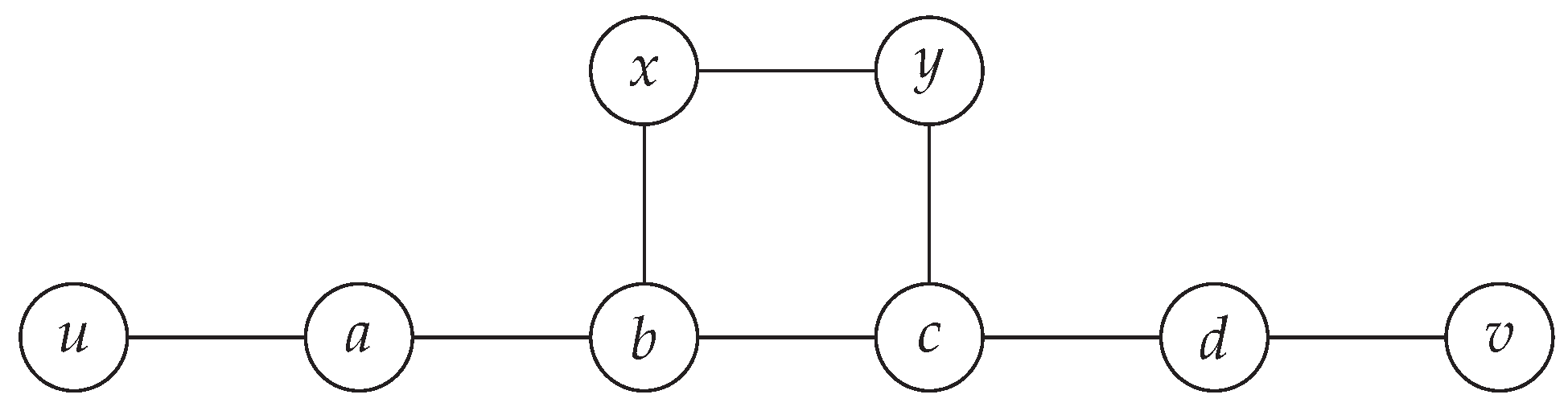

Table 1.
Notation.
| Symbol | Meaning |
|---|---|
| , n, m | The input graph, its number of vertices and its number of edges. |
| , , | Open and closed neighbourhood and degree of v. |
| , | Maximum and minimum degree. |
| Minimum size of an independent dominating set. | |
| , | Independence number and minimum vertex cover size. |
| S, | Output of Algorithm 1 and its approximation ratio. |
| Candidates of the strategies (Table 3). | |
| , , , P | Flags and penalty of the forest solver |
| (Section 3.2). | |
| IN, DOM, FREE | States of a vertex in the forest solver |
| (Section 3.2). | |
| , , | Terms of the recurrences of the forest solver |
| (Section 3.2). | |
| Degree threshold of the splitting strategy . | |
| The split vertices (Section 6). | |
| Splitting excess, . | |
| H (Section 6), | Copy graph of Algorithm 5 and decoded set. |
| H, , (Section 7) | A vertex cover instance, its number of edges, |
| and its VC-IDS graph. | |
| , N, q, W, | A formula, its numbers of variables and clauses, |
| its largest clause width, and its number of literal occurrences. | |
| Graph of with t copies of every clause | |
| (Definition 1). |
Table 2.
Code metadata of the siriaisa package. SciPy is used only by the experiment scripts, for the exact integer programs.
Table 2.
Code metadata of the siriaisa package. SciPy is used only by the experiment scripts, for the exact integer programs.
| Nr. | Code metadata description | Metadata |
|---|---|---|
| C1 | Current code version | v0.0.9 |
| C2 | Permanent link to code repository | https://github.com/frankvegadelgado/mids |
| C3 | Package name | siriaisa |
| C4 | Legal Code License | MIT License |
| C5 | Code versioning system used | git |
| C6 | Languages, tools, and services used | Python ≥ 3.12, NetworkX, NumPy, SciPy |
| C7 | Main entry points | iris, batch_iris, test_iris |
Table 3.
The eighteen strategies of Siriaisa 0.0.9. “Source” names the strategy of Salvador [21] or the phase of Esperanza [23] that it adapts.
| Name | Strategy | Source |
|---|---|---|
| spanning-tree peeling: maximum spanning forest, tree DP, peel, repeat | — | |
| endpoints of the NetworkX minimum maximal matching | Salvador | |
| greedy: the undominated vertex that dominates most undominated vertices | Salvador | |
| star-forest reduction solved by the tree DP | Salvador | |
| Min-to-Min | Salvador | |
| primal–dual on the domination linear program | Salvador | |
| BFS spanning forest solved by the tree DP | Salvador | |
| DFS spanning forest solved by the tree DP | Salvador | |
| induced-forest layers, each solved by the tree DP, in several orders | Salvador | |
| first forest layer re-solved exactly, the rest fixed from the best of – | Salvador, | |
| feedback-core peeling and the conditioned forest DP | Salvador | |
| dynamic minimum-degree (Caro–Wei) greedy | Esperanza baseline | |
| degree splitting at , decoding, repair | — | |
| union of –, repaired by votes | Salvador | |
| descent and weighted swap search from the best of – | Salvador, Esperanza | |
| reduce-and-search: swap search and forest large-neighbourhood search | Salvador | |
| consensus forcing over – | Salvador | |
| refinement of every candidate, a longer search on the best | Salvador, Esperanza |
Table 4.
The splitting excess () and the output on graph families. “Hardness” cites the hardness of MIDS on the family, or of the vertex cover problem it encodes; “Output” is the guarantee proved for Algorithm 1.
Table 4.
The splitting excess () and the output on graph families. “Hardness” cites the hardness of MIDS on the family, or of the vertex cover problem it encodes; “Output” is the guarantee proved for Algorithm 1.
| Family | Hardness | Output | |||
|---|---|---|---|---|---|
| cubic, | — | 3 | n | ratio | |
| cubic, | APX-hard [6] | 3 | 0 | ratio | |
| cubic planar, | NP-hard [5] | 3 | 0 | ratio | |
| cubic planar bipartite, | NP-complete [4] | 3 | 0 | ratio | |
| maximum degree | NP-hard within [10] | ; 0 for | ratio | ||
| maximum degree , bipartite or not, | NP-hard within [10] | 0 | ratio | ||
| SC-IDS of degree B, | reduction of [10] | B | 0 | ratio | |
| VC-IDS , , | vertex cover: UG-hard [18,28] | 0 | ratio | ||
| Khot–Regev YES graphs, | vertex cover: UG-hard [18] | 0 | — | ratio | |
| Khot–Regev YES graphs, any N | vertex cover: UG-hard [18] | — | ratio | ||
| planar, | NP-hard [5] | unbounded | ; for some graphs | — | — |
| bipartite planar, | NP-hard [4] | unbounded | ; for some graphs | — | — |
| circle graphs | not within , [3] | unbounded | up to (maximum) | — | — |
| — | unbounded | — | — | ||
| — | w.h.p. | 0 w.h.p. | — | ratio | |
| grids, ; hypercubes , | — | ; q | 0 | — | ratio |
| star , wheel | — | 1 | optimal | ||
| double star ( leaves) | — | optimal | |||
| complete graph | — | (maximum) | 1 | optimal | |
| complete bipartite , | — | b | optimal | ||
| complete multipartite | — | optimal | |||
| crown graph, | — | 2 | optimal | ||
| minimum degree | — | — | — |
Table 5.
The suite of graphs: number of instances, optimal outputs, mean and maximum ratio , the largest bound of Corollary 1 in the family, the mean maximum degree and the number of instances above the bound.
Table 5.
The suite of graphs: number of instances, optimal outputs, mean and maximum ratio , the largest bound of Corollary 1 in the family, the mean maximum degree and the number of instances above the bound.
| Family | Kind | Inst. | Opt. | Mean | Max | Bound | Mean | Viol. |
|---|---|---|---|---|---|---|---|---|
| clique | rigid | 667 | 667 | 1.0000 | 1.0000 | 1 | 6.47 | 0 |
| complete bipartite | rigid | 667 | 667 | 1.0000 | 1.0000 | 1 | 8.49 | 0 |
| crown | rigid | 666 | 666 | 1.0000 | 1.0000 | 1 | 3.09 | 0 |
| double star | rigid | 666 | 666 | 1.0000 | 1.0000 | 1 | 9.32 | 0 |
| star | rigid | 667 | 667 | 1.0000 | 1.0000 | 1 | 14.98 | 0 |
| balanced tree | bounded | 667 | 667 | 1.0000 | 1.0000 | 4 | 3.49 | 0 |
| cycle | bounded | 667 | 667 | 1.0000 | 1.0000 | 2 | 2.00 | 0 |
| grid | bounded | 667 | 667 | 1.0000 | 1.0000 | 4 | 3.60 | 0 |
| ladder | bounded | 667 | 667 | 1.0000 | 1.0000 | 3 | 2.95 | 0 |
| lollipop | bounded | 667 | 667 | 1.0000 | 1.0000 | 8 | 5.52 | 0 |
| path | bounded | 667 | 667 | 1.0000 | 1.0000 | 2 | 1.98 | 0 |
| random regular | bounded | 667 | 667 | 1.0000 | 1.0000 | 5 | 3.53 | 0 |
| Barabási–Albert | random | 666 | 665 | 1.0003 | 1.2000 | 21 | 8.91 | 0 |
| Erdos–Rényi | random | 666 | 666 | 1.0000 | 1.0000 | 20 | 8.07 | 0 |
| random tree | random | 666 | 666 | 1.0000 | 1.0000 | 7 | 3.77 | 0 |
| All | 10000 | 9999 | 1.0000 | 1.2000 | 0 |
Table 6.
Siriaisa and four baseline heuristics on the suite of graphs: number of optimal outputs (Opt.) and mean and maximum ratio to the optimum (file car_baselines_summary.csv).
Table 6.
Siriaisa and four baseline heuristics on the suite of graphs: number of optimal outputs (Opt.) and mean and maximum ratio to the optimum (file car_baselines_summary.csv).
| Siriaisa | Random maximal | Min-degree greedy | Max-degree greedy | Max-degree + 2-swap | ||||||||||||
|---|---|---|---|---|---|---|---|---|---|---|---|---|---|---|---|---|
| Family | Inst. | Opt. | Mean | Max | Opt. | Mean | Max | Opt. | Mean | Max | Opt. | Mean | Max | Opt. | Mean | Max |
| balanced_tree | 667 | 667 | 1.000 | 1.000 | 12 | 2.150 | 3.333 | 0 | 2.658 | 3.333 | 329 | 1.203 | 1.400 | 329 | 1.203 | 1.400 |
| barabasi_albert | 666 | 665 | 1.000 | 1.200 | 44 | 1.684 | 6.000 | 3 | 1.921 | 6.000 | 452 | 1.089 | 2.000 | 474 | 1.079 | 2.000 |
| clique | 667 | 667 | 1.000 | 1.000 | 667 | 1.000 | 1.000 | 667 | 1.000 | 1.000 | 667 | 1.000 | 1.000 | 667 | 1.000 | 1.000 |
| complete_bipartite | 667 | 667 | 1.000 | 1.000 | 250 | 2.352 | 12.000 | 57 | 2.646 | 12.000 | 667 | 1.000 | 1.000 | 667 | 1.000 | 1.000 |
| crown | 666 | 666 | 1.000 | 1.000 | 251 | 1.811 | 3.000 | 117 | 2.045 | 3.000 | 666 | 1.000 | 1.000 | 666 | 1.000 | 1.000 |
| cycle | 667 | 667 | 1.000 | 1.000 | 124 | 1.210 | 1.500 | 70 | 1.356 | 1.500 | 667 | 1.000 | 1.000 | 667 | 1.000 | 1.000 |
| double_star | 666 | 666 | 1.000 | 1.000 | 100 | 2.305 | 6.500 | 5 | 2.599 | 6.500 | 666 | 1.000 | 1.000 | 666 | 1.000 | 1.000 |
| erdos_renyi | 666 | 666 | 1.000 | 1.000 | 71 | 1.472 | 2.667 | 27 | 1.704 | 3.000 | 332 | 1.146 | 2.000 | 417 | 1.095 | 2.000 |
| grid | 667 | 667 | 1.000 | 1.000 | 123 | 1.361 | 2.000 | 24 | 1.629 | 2.000 | 111 | 1.309 | 1.667 | 248 | 1.197 | 1.667 |
| ladder | 667 | 667 | 1.000 | 1.000 | 72 | 1.439 | 1.857 | 33 | 1.673 | 1.889 | 75 | 1.268 | 1.500 | 260 | 1.117 | 1.333 |
| lollipop | 667 | 667 | 1.000 | 1.000 | 165 | 1.325 | 2.000 | 47 | 1.472 | 2.000 | 667 | 1.000 | 1.000 | 667 | 1.000 | 1.000 |
| path | 667 | 667 | 1.000 | 1.000 | 90 | 1.277 | 2.000 | 31 | 1.459 | 2.000 | 667 | 1.000 | 1.000 | 667 | 1.000 | 1.000 |
| random_tree | 666 | 666 | 1.000 | 1.000 | 94 | 1.373 | 3.000 | 40 | 1.548 | 3.000 | 385 | 1.075 | 2.000 | 468 | 1.046 | 1.667 |
| regular | 667 | 667 | 1.000 | 1.000 | 147 | 1.274 | 2.500 | 99 | 1.417 | 2.500 | 244 | 1.161 | 1.750 | 390 | 1.081 | 1.667 |
| star | 667 | 667 | 1.000 | 1.000 | 91 | 14.063 | 30.000 | 33 | 14.979 | 30.000 | 667 | 1.000 | 1.000 | 667 | 1.000 | 1.000 |
| All | 10000 | 9999 | 1.000 | 1.200 | 2301 | 2.407 | 30.000 | 1253 | 2.674 | 30.000 | 7262 | 1.083 | 2.000 | 7920 | 1.055 | 2.000 |
Table 7.
Bipartite graphs: instances, instances with the optimum proved (“Ref.”), optimal, suboptimal and open outputs, maximum and mean ratio (certified upper bounds on open instances), and the time of Siriaisa in seconds.
Table 7.
Bipartite graphs: instances, instances with the optimum proved (“Ref.”), optimal, suboptimal and open outputs, maximum and mean ratio (certified upper bounds on open instances), and the time of Siriaisa in seconds.
| Family | Inst. | Ref. | Opt. | Subopt. | Open | Max ratio | Mean ratio | Time |
|---|---|---|---|---|---|---|---|---|
| 2D grid | 2 | 2 | 2 | 0 | 0 | 1.0000 | 1.0000 | 4.8 |
| 2D grid, 70% edges kept | 6 | 6 | 6 | 0 | 0 | 1.0000 | 1.0000 | 30.0 |
| 3D grid | 2 | 1 | 1 | 0 | 1 | 1.0750 | 1.0375 | 5.6 |
| complete bipartite | 2 | 2 | 2 | 0 | 0 | 1.0000 | 1.0000 | 3.4 |
| crown graph | 2 | 2 | 2 | 0 | 0 | 1.0000 | 1.0000 | 0.2 |
| double cover of random regular | 12 | 8 | 8 | 0 | 4 | 1.1765 | 1.0370 | 46.9 |
| even cycle | 2 | 2 | 2 | 0 | 0 | 1.0000 | 1.0000 | 0.0 |
| hidden perfect matching + random edges | 12 | 12 | 12 | 0 | 0 | 1.0000 | 1.0000 | 42.3 |
| hypercube | 2 | 2 | 2 | 0 | 0 | 1.0000 | 1.0000 | 4.9 |
| hypercube, 50% edges kept | 2 | 2 | 2 | 0 | 0 | 1.0000 | 1.0000 | 10.9 |
| path | 2 | 2 | 2 | 0 | 0 | 1.0000 | 1.0000 | 0.0 |
| power-law bipartite | 6 | 6 | 6 | 0 | 0 | 1.0000 | 1.0000 | 25.1 |
| random bipartite (1:2) | 18 | 15 | 15 | 0 | 3 | 1.4545 | 1.0657 | 56.9 |
| random bipartite (balanced) | 18 | 15 | 15 | 0 | 3 | 1.4167 | 1.0602 | 60.7 |
| random d-regular bipartite | 18 | 12 | 12 | 0 | 6 | 1.2917 | 1.0623 | 78.9 |
| random tree | 6 | 6 | 6 | 0 | 0 | 1.0000 | 1.0000 | 20.3 |
| All | 112 | 95 | 95 | 0 | 17 | 1.4545 | 1.0349 | 391.0 |
Table 8.
Instances of the reductions of Chlebík and Chlebíková. “Ref.” counts instances with i proved; “Opt.”, “Subopt.” and “Open” classify against it; “max ” is the largest certified ratio, “max exc.” the largest ; the last two columns give the number of optimal decoded covers and the largest .
Table 8.
Instances of the reductions of Chlebík and Chlebíková. “Ref.” counts instances with i proved; “Opt.”, “Subopt.” and “Open” classify against it; “max ” is the largest certified ratio, “max exc.” the largest ; the last two columns give the number of optimal decoded covers and the largest .
| Family | Inst. | n | Ref. | Opt. | Subopt. | Open | max | max exc. | opt. / max | |
|---|---|---|---|---|---|---|---|---|---|---|
| SC-IDS, | 6 | 113–225 | 4 | 6 | 6 | 0 | 0 | 1.0000 | 0 | — |
| SC-IDS, | 6 | 108–228 | 5 | 6 | 6 | 0 | 0 | 1.0000 | 0 | — |
| SC-IDS, | 6 | 106–224 | 6 | 6 | 6 | 0 | 0 | 1.0000 | 0 | — |
| VC-IDS, 3-regular H | 9 | 500–2 000 | 3 | 9 | 1 | 8 | 0 | 1.0309 | 22 | 1 / 1.1982 |
| VC-IDS, 4-regular H | 9 | 650–2 600 | 4 | 8 | 1 | 7 | 1 | 1.0360 | 33 | 1 / 1.2821 |
| VC-IDS, 5-regular H | 9 | 800–3 200 | 5 | 6 | 0 | 6 | 3 | 1.0375 | 42 | 0 / 1.3500 |
| VC-IDS, Khot–Regev H | 10 | 48 172–75 166 | 64 | 7 | 0 | 7 | 3 | 1.0175 | 292 | 0 / 1.8665 |
| All | 55 | 48 | 20 | 28 | 7 | 1.0375 | 292 | 2 / 1.8665 |
Table 9.
Splitting excess on hard and structured families (): largest maximum degree, instances with , largest and , and instances on which the decoded set of some inner solver is independent. “Ref.” counts instances with proved (integer program, closed form, planted value or reduction identity); “Opt.”, “Subopt.” and “Open” classify the output against it; “Max ratio” is the largest for the certified lower bound L (an upper bound on the ratio of open instances); “Time” is the total time of Siriaisa in seconds. *Union of d random perfect matchings with repeated edges merged (maximum degree d).
Table 9.
Splitting excess on hard and structured families (): largest maximum degree, instances with , largest and , and instances on which the decoded set of some inner solver is independent. “Ref.” counts instances with proved (integer program, closed form, planted value or reduction identity); “Opt.”, “Subopt.” and “Open” classify the output against it; “Max ratio” is the largest for the certified lower bound L (an upper bound on the ratio of open instances); “Time” is the total time of Siriaisa in seconds. *Union of d random perfect matchings with repeated edges merged (maximum degree d).
| Family | Inst. | n | max s | max | ind. | Ref. | Opt. | Subopt. | Open | Max ratio | Time | ||
|---|---|---|---|---|---|---|---|---|---|---|---|---|---|
| random 3-regular bipartite* | 4 | 100–400 | 3 | 4 | 0 | 0.000 | 4 | 2 | 2 | 0 | 2 | 1.0784 | 38.0 |
| planar (Delaunay) | 4 | 100–400 | 12 | 4 | 0 | 0.000 | 4 | 4 | 3 | 1 | 0 | 1.0161 | 33.3 |
| random 4-regular | 4 | 100–400 | 4 | 4 | 0 | 0.000 | 4 | 2 | 2 | 0 | 2 | 1.1481 | 35.5 |
| random 5-regular | 4 | 100–400 | 5 | 4 | 0 | 0.000 | 4 | 2 | 2 | 0 | 2 | 1.2239 | 34.5 |
| random 6-regular | 4 | 100–400 | 6 | 4 | 0 | 0.000 | 4 | 2 | 2 | 0 | 2 | 1.2586 | 36.3 |
| random 4-regular bipartite* | 4 | 100–400 | 4 | 4 | 0 | 0.000 | 4 | 2 | 2 | 0 | 2 | 1.1481 | 32.3 |
| random 5-regular bipartite* | 4 | 100–400 | 5 | 4 | 0 | 0.000 | 4 | 2 | 2 | 0 | 2 | 1.2059 | 30.0 |
| SC-IDS, | 4 | 94–375 | 4 | 4 | 0 | 0.000 | 4 | 4 | 3 | 1 | 0 | 1.0080 | 33.0 |
| SC-IDS, | 4 | 93–384 | 6 | 4 | 0 | 0.000 | 4 | 4 | 4 | 0 | 0 | 1.0000 | 25.0 |
| VC-IDS, 3-regular H | 4 | 240–1 000 | 3 | 4 | 0 | 0.000 | 4 | 2 | 2 | 0 | 2 | 1.4400 | 59.2 |
| 4 | 100–400 | 230 | 0 | 3 783 | 0.473 | 0 | 2 | 2 | 0 | 2 | 2.5000 | 19.5 | |
| complete | 4 | 100–400 | 399 | 0 | 7 600 | 0.950 | 0 | 4 | 4 | 0 | 0 | 1.0000 | 4.9 |
| 4 | 100–400 | 200 | 0 | 3 600 | 0.450 | 4 | 4 | 4 | 0 | 0 | 1.0000 | 19.0 | |
| 4 | 100–400 | 300 | 0 | 2 600 | 0.325 | 2 | 4 | 4 | 0 | 0 | 1.0000 | 13.8 | |
| complete 4-partite, equal parts | 4 | 100–400 | 300 | 0 | 5 600 | 0.700 | 0 | 4 | 4 | 0 | 0 | 1.0000 | 22.0 |
| complete 5-partite, random parts | 4 | 100–400 | 392 | 0 | 5 889 | 0.736 | 0 | 4 | 4 | 0 | 0 | 1.0000 | 17.8 |
| crown | 4 | 100–400 | 199 | 0 | 3 600 | 0.450 | 0 | 4 | 4 | 0 | 0 | 1.0000 | 2.8 |
| star | 4 | 100–400 | 399 | 0 | 19 | 0.009 | 4 | 4 | 4 | 0 | 0 | 1.0000 | 0.1 |
| wheel | 4 | 100–400 | 399 | 0 | 19 | 0.009 | 4 | 4 | 4 | 0 | 0 | 1.0000 | 0.2 |
| double star | 4 | 100–400 | 200 | 0 | 18 | 0.008 | 0 | 4 | 4 | 0 | 0 | 1.0000 | 25.3 |
| split graph | 4 | 100–400 | 232 | 0 | 209 | 0.055 | 0 | 4 | 4 | 0 | 0 | 1.0000 | 7.7 |
| 4 | 100–400 | 11 | 4 | 0 | 0.000 | 4 | 4 | 3 | 1 | 0 | 1.0075 | 47.6 | |
| Barabási–Albert, | 4 | 100–400 | 67 | 0 | 19 | 0.013 | 0 | 4 | 2 | 2 | 0 | 1.0532 | 25.8 |
| power-law bipartite | 4 | 100–400 | 55 | 0 | 6 | 0.004 | 1 | 4 | 4 | 0 | 0 | 1.0000 | 43.9 |
| 2D grid | 4 | 100–400 | 4 | 4 | 0 | 0.000 | 4 | 2 | 2 | 0 | 2 | 1.0814 | 31.2 |
| hypercube | 2 | 128–512 | 9 | 2 | 0 | 0.000 | 2 | 1 | 1 | 0 | 1 | 1.2308 | 4.8 |
| Khot–Regev YES | 2 | 640 | 64 | 0 | 323 | 0.020 | 0 | 0 | 0 | 0 | 2 | 15.9000 | 10.2 |
| Khot–Regev YES, , | 4 | 160–320 | 24 | 2 | 39 | 0.007 | 2 | 4 | 1 | 3 | 0 | 1.0361 | 23.7 |
| VC-IDS, Khot–Regev H | 2 | 49 096–51 550 | 64 | 2 | 0 | 0.000 | 2 | 0 | 0 | 0 | 2 | 22.1825 | 87.0 |
| All | 110 | 54 | 7 600 | 0.950 | 69 | 87 | 79 | 8 | 23 | 22.1825 | 764.3 |
Table 10.
Cubic and subcubic graphs: the values of , instances on which the copy graph is G (no vertex split), the classification of the output, and the largest . “Ref.” counts instances with proved (integer program, closed form, planted value or reduction identity); “Opt.”, “Subopt.” and “Open” classify the output against it; “Max ratio” is the largest for the certified lower bound L (an upper bound on the ratio of open instances); “Time” is the total time of Siriaisa in seconds. †Petersen, Heawood, Möbius–Kantor, Pappus, Desargues, dodecahedron, truncated tetrahedron, truncated cube, Frucht, Tutte, McGee and Foster graphs.
Table 10.
Cubic and subcubic graphs: the values of , instances on which the copy graph is G (no vertex split), the classification of the output, and the largest . “Ref.” counts instances with proved (integer program, closed form, planted value or reduction identity); “Opt.”, “Subopt.” and “Open” classify the output against it; “Max ratio” is the largest for the certified lower bound L (an upper bound on the ratio of open instances); “Time” is the total time of Siriaisa in seconds. †Petersen, Heawood, Möbius–Kantor, Pappus, Desargues, dodecahedron, truncated tetrahedron, truncated cube, Frucht, Tutte, McGee and Foster graphs.
| Family | Inst. | n | Ref. | Opt. | Subopt. | Open | Max ratio | max | Time | ||
|---|---|---|---|---|---|---|---|---|---|---|---|
| cubic, | 1 | 4 | 4 | 0 | 1 | 1 | 0 | 0 | 1.0000 | 0.2500 | 0.0 |
| cubic, | 2 | 6 | 6 | 0 | 2 | 2 | 0 | 0 | 1.0000 | 0.5000 | 0.0 |
| cubic, | 6 | 8 | 8 | 0 | 6 | 6 | 0 | 0 | 1.0000 | 0.3750 | 0.0 |
| , | 6 | 3–8 | 1,4,5,6 | 0 | 6 | 6 | 0 | 0 | 1.0000 | 0.4000 | 0.0 |
| named cubic | 12 | 10–90 | 0 | 12 | 12 | 12 | 0 | 0 | 1.0000 | 0.3333 | 2.1 |
| random cubic | 4 | 100–400 | 0 | 4 | 2 | 2 | 0 | 2 | 1.0693 | 0.2700 | 19.6 |
| random cubic bipartite | 4 | 100–400 | 0 | 4 | 2 | 2 | 0 | 2 | 1.0693 | 0.2700 | 25.1 |
| double cover of random cubic | 4 | 100–400 | 0 | 4 | 2 | 2 | 0 | 2 | 1.0693 | 0.2800 | 24.5 |
| cubic planar (dual of Delaunay) | 4 | 100–400 | 0 | 4 | 2 | 2 | 0 | 2 | 1.0792 | 0.2725 | 25.0 |
| cubic planar bipartite | 4 | 100–400 | 0 | 4 | 2 | 2 | 0 | 2 | 1.0588 | 0.2800 | 20.8 |
| random cubic, edges deleted | 4 | 100–400 | 0 | 4 | 4 | 4 | 0 | 0 | 1.0000 | 0.3250 | 25.1 |
| prism | 4 | 100–402 | 0 | 4 | 3 | 3 | 0 | 1 | 1.0099 | 0.2600 | 13.2 |
| Möbius ladder | 2 | 100–400 | 0 | 2 | 2 | 2 | 0 | 0 | 1.0000 | 0.2525 | 10.3 |
| generalized Petersen | 2 | 100–400 | 0 | 2 | 1 | 1 | 0 | 1 | 1.1650 | 0.3000 | 11.7 |
| generalized Petersen | 2 | 100–400 | 0 | 2 | 2 | 2 | 0 | 0 | 1.0000 | 0.2600 | 5.2 |
| All | 61 | 46 | 49 | 49 | 0 | 12 | 1.1650 | 0.5000 | 182.7 |
Table 11.
Circle graphs built from chord models: largest number of edges and maximum degree, instances with , largest and , instances with an independent decoded set . “Ref.” counts instances with proved (integer program, closed form, planted value or reduction identity); “Opt.”, “Subopt.” and “Open” classify the output against it; “Max ratio” is the largest for the certified lower bound L (an upper bound on the ratio of open instances); “Time” is the total time of Siriaisa in seconds.
Table 11.
Circle graphs built from chord models: largest number of edges and maximum degree, instances with , largest and , instances with an independent decoded set . “Ref.” counts instances with proved (integer program, closed form, planted value or reduction identity); “Opt.”, “Subopt.” and “Open” classify the output against it; “Max ratio” is the largest for the certified lower bound L (an upper bound on the ratio of open instances); “Time” is the total time of Siriaisa in seconds.
| Family | Inst. | n | max m | max s | max | ind. | Ref. | Opt. | Subopt. | Open | Max ratio | Time | ||
|---|---|---|---|---|---|---|---|---|---|---|---|---|---|---|
| uniform random chords | 4 | 100–400 | 27 268 | 219 | 0 | 2 513 | 0.331 | 0 | 2 | 2 | 0 | 2 | 1.1905 | 6.5 |
| short chords, degree | 4 | 100–400 | 904 | 14 | 3 | 2 | 0.002 | 3 | 4 | 4 | 0 | 0 | 1.0000 | 19.4 |
| short chords, degree | 4 | 100–400 | 2 500 | 29 | 0 | 107 | 0.119 | 0 | 4 | 2 | 2 | 0 | 1.0405 | 12.5 |
| short chords, degree | 4 | 100–400 | 5 488 | 57 | 0 | 354 | 0.092 | 0 | 4 | 2 | 2 | 0 | 1.0600 | 8.6 |
| permutation graph | 4 | 100–400 | 41 274 | 393 | 0 | 3 925 | 0.563 | 0 | 4 | 4 | 0 | 0 | 1.0000 | 11.0 |
| 2 hub chords | 4 | 100–400 | 532 | 102 | 0 | 15 | 0.007 | 1 | 4 | 4 | 0 | 0 | 1.0000 | 16.5 |
| 4 hub chords | 4 | 100–400 | 599 | 54 | 0 | 14 | 0.006 | 1 | 4 | 4 | 0 | 0 | 1.0000 | 16.9 |
| diameters () | 2 | 100–400 | 79 800 | 399 | 0 | 7 600 | 1.000 | 0 | 2 | 2 | 0 | 0 | 1.0000 | 0.8 |
| 2 | 100–400 | 40 000 | 200 | 0 | 3 600 | 0.474 | 2 | 2 | 2 | 0 | 0 | 1.0000 | 4.4 | |
| 2 | 100–400 | 30 000 | 300 | 0 | 2 600 | 0.361 | 1 | 2 | 2 | 0 | 0 | 1.0000 | 5.0 | |
| star | 2 | 100–400 | 399 | 399 | 0 | 19 | 0.010 | 2 | 2 | 2 | 0 | 0 | 1.0000 | 0.0 |
| path | 2 | 100–400 | 399 | 2 | 2 | 0 | 0.000 | 2 | 2 | 2 | 0 | 0 | 1.0000 | 0.0 |
| cycle | 2 | 100–400 | 400 | 2 | 2 | 0 | 0.000 | 2 | 2 | 2 | 0 | 0 | 1.0000 | 0.1 |
| All | 40 | 7 | 7 600 | 1.000 | 14 | 38 | 34 | 4 | 2 | 1.1905 | 101.7 |
Table 12.
Graphs of maximum degree B with , on which : instances, number of vertices and largest number of edges, instances with , the classification of the output, and the largest and mean . “Ref.” counts instances with proved (integer program, closed form, planted value or reduction identity); “Opt.”, “Subopt.” and “Open” classify the output against it; “Max ratio” is the largest for the certified lower bound L (an upper bound on the ratio of open instances); “Time” is the total time of Siriaisa in seconds.
Table 12.
Graphs of maximum degree B with , on which : instances, number of vertices and largest number of edges, instances with , the classification of the output, and the largest and mean . “Ref.” counts instances with proved (integer program, closed form, planted value or reduction identity); “Opt.”, “Subopt.” and “Open” classify the output against it; “Max ratio” is the largest for the certified lower bound L (an upper bound on the ratio of open instances); “Time” is the total time of Siriaisa in seconds.
| Family | B | Inst. | n | max m | Ref. | Opt. | Subopt. | Open | Max ratio | Mean ratio | Time | |
|---|---|---|---|---|---|---|---|---|---|---|---|---|
| random B-regular | 4 | 2 | 256 | 512 | 2 | 0 | 0 | 0 | 2 | 1.1346 | 1.1346 | 10.9 |
| random B-regular bipartite (double cover) | 4 | 2 | 256 | 512 | 2 | 0 | 0 | 0 | 2 | 1.1154 | 1.1058 | 10.9 |
| B-regular, planted perfect code | 4 | 2 | 260 | 520 | 2 | 2 | 2 | 0 | 0 | 1.0000 | 1.0000 | 1.1 |
| SC-IDS | 4 | 2 | 323 | 430 | 2 | 2 | 2 | 0 | 0 | 1.0000 | 1.0000 | 18.4 |
| VC-IDS, B-regular H | 4 | 2 | 260 | 320 | 2 | 2 | 2 | 0 | 0 | 1.0000 | 1.0000 | 20.0 |
| random B-regular | 8 | 2 | 256 | 1 024 | 2 | 0 | 0 | 0 | 2 | 1.3793 | 1.3621 | 8.5 |
| random B-regular bipartite (double cover) | 8 | 2 | 256 | 1 024 | 2 | 0 | 0 | 0 | 2 | 1.3448 | 1.3448 | 6.7 |
| B-regular, planted perfect code | 8 | 2 | 261 | 1 044 | 2 | 2 | 2 | 0 | 0 | 1.0000 | 1.0000 | 0.6 |
| SC-IDS | 8 | 2 | 331–334 | 769 | 2 | 2 | 2 | 0 | 0 | 1.0000 | 1.0000 | 13.5 |
| VC-IDS, B-regular H | 8 | 2 | 250 | 320 | 2 | 2 | 2 | 0 | 0 | 1.0000 | 1.0000 | 24.8 |
| random B-regular | 16 | 2 | 256 | 2 048 | 2 | 0 | 0 | 0 | 2 | 1.5625 | 1.5312 | 4.0 |
| random B-regular bipartite (double cover) | 16 | 2 | 256 | 2 048 | 2 | 0 | 0 | 0 | 2 | 1.5625 | 1.5625 | 5.0 |
| B-regular, planted perfect code | 16 | 2 | 272 | 2 176 | 2 | 2 | 2 | 0 | 0 | 1.0000 | 1.0000 | 0.7 |
| SC-IDS | 16 | 2 | 318–321 | 1 353 | 2 | 2 | 0 | 2 | 0 | 1.0115 | 1.0114 | 11.4 |
| VC-IDS, B-regular H | 16 | 2 | 882 | 1 152 | 2 | 2 | 1 | 1 | 0 | 1.0033 | 1.0016 | 19.8 |
| random B-regular | 32 | 2 | 1 024 | 16 384 | 2 | 0 | 0 | 0 | 2 | 2.2188 | 2.2188 | 5.8 |
| random B-regular bipartite (double cover) | 32 | 2 | 1 024 | 16 384 | 2 | 0 | 0 | 0 | 2 | 2.2500 | 2.2500 | 4.2 |
| B-regular, planted perfect code | 32 | 2 | 1 056 | 16 896 | 2 | 2 | 2 | 0 | 0 | 1.0000 | 1.0000 | 1.5 |
| SC-IDS | 32 | 2 | 1 313 | 10 787 | 2 | 0 | 0 | 0 | 2 | 1.0562 | 1.0533 | 7.1 |
| VC-IDS, B-regular H | 32 | 2 | 3 298 | 4 352 | 2 | 2 | 0 | 2 | 0 | 1.0009 | 1.0009 | 13.1 |
| Khot–Regev YES, , | 12 | 2 | 160 | 382 | 2 | 2 | 1 | 1 | 0 | 1.0364 | 1.0182 | 10.6 |
| Khot–Regev YES, , | 24 | 2 | 608 | 2 938 | 2 | 2 | 0 | 2 | 0 | 1.0237 | 1.0149 | 11.2 |
| All | 44 | 44 | 26 | 18 | 8 | 18 | 2.2500 | 1.2095 | 209.7 |
Table 13.
Complements of the DIMACS clique benchmark graphs: size of the returned set and time of Siriaisa in seconds.
Table 13.
Complements of the DIMACS clique benchmark graphs: size of the returned set and time of Siriaisa in seconds.
| Instance | Time | Instance | Time | ||
|---|---|---|---|---|---|
| brock200_1 | 8 | 1.01 | brock200_2 | 4 | 1.28 |
| brock200_3 | 5 | 1.07 | brock200_4 | 6 | 1.09 |
| brock400_1 | 10 | 1.66 | brock400_2 | 11 | 1.52 |
| brock400_3 | 11 | 1.54 | brock400_4 | 11 | 1.61 |
| brock800_1 | 8 | 7.39 | brock800_2 | 9 | 6.74 |
| brock800_3 | 9 | 7.11 | brock800_4 | 9 | 10.11 |
| c-fat200-1 | 10 | 2.27 | c-fat200-2 | 22 | 2.35 |
| c-fat200-5 | 56 | 2.58 | c-fat500-1 | 12 | 11.69 |
| c-fat500-10 | 124 | 7.12 | c-fat500-2 | 24 | 11.85 |
| c-fat500-5 | 62 | 8.88 | C1000.9 | 31 | 6.95 |
| C125.9 | 14 | 3.50 | C250.9 | 18 | 2.35 |
| C500.9 | 25 | 2.87 | gen200_p0.9_44 | 16 | 2.55 |
| gen200_p0.9_55 | 16 | 2.82 | gen400_p0.9_55 | 21 | 2.50 |
| gen400_p0.9_65 | 22 | 2.53 | gen400_p0.9_75 | 24 | 2.41 |
| hamming10-2 | 128 | 5.12 | hamming10-4 | 13 | 9.62 |
| hamming6-2 | 12 | 1.74 | hamming6-4 | 2 | 0.10 |
| hamming8-2 | 32 | 4.48 | hamming8-4 | 4 | 4.11 |
| johnson16-2-4 | 8 | 3.09 | johnson32-2-4 | 16 | 3.61 |
| johnson8-2-4 | 4 | 1.13 | johnson8-4-4 | 7 | 4.07 |
| keller4 | 5 | 2.83 | keller5 | 10 | 9.46 |
| MANN_a27 | 27 | 0.14 | MANN_a45 | 45 | 0.20 |
| MANN_a81 | 81 | 0.35 | MANN_a9 | 9 | 0.03 |
| p_hat1000-3 | 15 | 7.82 | p_hat300-1 | 3 | 2.09 |
| p_hat300-2 | 5 | 1.59 | p_hat300-3 | 10 | 1.13 |
| p_hat500-1 | 3 | 4.98 | p_hat500-2 | 7 | 3.96 |
| p_hat500-3 | 11 | 2.12 | p_hat700-1 | 3 | 9.54 |
| p_hat700-2 | 7 | 7.03 | p_hat700-3 | 14 | 3.97 |
| san200_0.7_1 | 7 | 1.05 | san200_0.7_2 | 6 | 1.23 |
| san200_0.9_1 | 16 | 1.56 | san200_0.9_2 | 16 | 1.48 |
| san200_0.9_3 | 15 | 1.47 | san400_0.5_1 | 4 | 2.64 |
| san400_0.7_1 | 8 | 1.95 | san400_0.7_2 | 8 | 2.03 |
| san400_0.7_3 | 8 | 2.01 | san400_0.9_1 | 22 | 1.43 |
| sanr200_0.7 | 7 | 1.06 | sanr200_0.9 | 16 | 1.45 |
| sanr400_0.5 | 5 | 2.78 | sanr400_0.7 | 9 | 2.25 |
Disclaimer/Publisher’s Note: The statements, opinions and data contained in all publications are solely those of the individual author(s) and contributor(s) and not of MDPI and/or the editor(s). MDPI and/or the editor(s) disclaim responsibility for any injury to people or property resulting from any ideas, methods, instructions or products referred to in the content. |
© 2026 by the author. Licensee MDPI, Basel, Switzerland. This article is an open access article distributed under the terms and conditions of the Creative Commons Attribution (CC BY) license.
Copyright: This open access article is published under a Creative Commons CC BY 4.0 license, which permit the free download, distribution, and reuse, provided that the author and preprint are cited in any reuse.