

Submitted:
01 July 2026
Posted:
02 July 2026
You are already at the latest version
Abstract
The Minimum Independent Dominating Set problem (MIDS), equivalently the problem of finding a smallest maximal independent set, is strongly inapproximable: unless P = NP, no polynomial-time algorithm approximates it within any fixed constant factor. This rules out a single universal constant, but it does not rule out constant factors that are specific to structured graph classes. This manuscript studies Siriaisa, the unweighted MIDS algorithm distributed as the siriaisa package, and proves such family-restricted guarantees. Siriaisa removes isolated vertices, processes each component independently, solves an LP relaxation whose values serve only as priority scores for a maximal-independent-set sweep; for every component it assembles a deterministic pool of candidates (two lifted degree-four seeds, the direct LP sweep, six fixed orderings, and single- and paired-seed sweeps) and shrinks each feasible candidate by a bounded local-exchange compression built from reverse-delete and one-add/two-add exchanges, returning the smallest verified independent dominating set. We give two unconditional guarantees. First, every returned set is independent and dominating. Second, because every returned component set is a maximal independent set, it is a ∆-approximation of the component optimum; hence Siriaisa is a constant-factor approximation on every bounded-degree family (factor 2 for paths and cycles, 3 for ladders, 4 for grids, r for r-regular graphs), and it returns the exact optimum, ratio 1, on structurally rigid families of unbounded degree: cliques, stars, complete bipartite graphs, and double stars for all parameters, and crown graphs within the seed-pool range. A separate consequence of the compression is that every returned set is reverse-delete minimal and locally optimal under the implemented one-add and two-add exchanges. We make explicit what is not claimed: the LP ordering carries no universal approximation guarantee, and a universal constant factor would contradict Irving’s theorem unless P = NP, so we claim no graph-independent constant. We validate the theory against exact SciPy MILP optima on a small adversarial DIMACS suite and on a large-scale reproducible harness, the car suite, that runs ten thousand instances across the structured families and random graphs: every instance stays within its family constant, 99.85% are solved exactly, and the largest ratio across the whole suite is 1.20.
Keywords:
minimum independent dominating set
; minimum maximal independent set
; approximation algorithm
; linear programming
; P vs. NP
MSC: 05C69; 68Q25; 90C27
1. Introduction
An independent dominating set of an undirected graph is a set that is both independent and dominating: no two vertices of D are adjacent, and every vertex of has at least one neighbour in D. Equivalently, D is a maximal independent set. The Minimum Independent Dominating Set problem asks for such a set of minimum cardinality, denoted . MIDS is much harder to approximate than the ordinary Minimum Dominating Set problem. Irving proved that, unless , no polynomial-time algorithm can guarantee a factor K for any fixed constant [1]. Halldorsson later strengthened the lower bound for the equivalent minimum maximal independent set formulation [2]. Thus a polynomial-time fixed-constant approximation for MIDS is not merely a new approximation result: combined with the known hardness theorem, it would imply . This paper documents the current unweighted implementation in the mids repository, called Siriaisa. The algorithm is built around three ideas.
- 1.
- It uses an LP relaxation of unweighted MIDS, with domination constraints on closed neighbourhoods and independence constraints on edges.
- 2.
- It reduces an arbitrary component to an auxiliary graph whose maximum degree is at most four, then uses the LP values as priority scores for a maximal-independent-set sweep (an ordering, not an LP rounding in the usual sense).
- 3.
- It lifts the reduced solution back to the original component in two polarities, repairs both lifted vertex seeds into maximal independent sets, and compares them with the LP-guided maximal independent set on the original component.
The implementation repairs and validates every candidate before returning it. This is important because the degree-four gadget may produce a valid independent dominating set in the auxiliary graph whose first-coordinate projection is no longer independent in the original graph; Remark 1 explains why the lifted seeds are repaired before selection.
Contributions
The main contributions of this manuscript are the following.
- A source-faithful description of the current Siriaisa implementation for unweighted MIDS.
- Pseudocode for the LP-guided greedy routine, the degree-four gadget, the seed repair, the deterministic candidate pool, the reverse-delete and local-exchange compression, and the multi-candidate component selector.
- A TikZ depiction of the degree-four replacement gadget.
- A correctness proof showing that every returned set is an independent dominating set, and an implemented local-optimality theorem: every returned set is reverse-delete minimal and locally optimal under the one-add and two-add exchanges.
- A proof that the sequential degree-four gadget produces an auxiliary graph of maximum degree at most four and linear size.
- A worst-case running-time analysis, dominated by the verified two-add exchange phase, that is polynomial but explicitly not linear.
- Two unconditional structural approximation theorems: every returned component set is a maximal independent set and hence a -approximation, which gives a constant factor on every bounded-degree family; and exact optimality on the rigid families (cliques, stars, complete bipartite graphs, crowns, and double stars).
- An explicit and honest delineation of the limits: the LP ordering carries no universal approximation guarantee, and any universal constant factor would imply , so no graph-independent constant is claimed.
- Two reproducible experiments validated against exact SciPy MILP optima: the archived adversarial DIMACS suite, and the large-scale car suite of ten thousand instances across the structured families and random graphs.
The paper is organised as follows. Section 2 records the implementation metadata. Section 3 describes the algorithm and the degree-four gadget. Section 4 proves feasibility and the implemented local-optimality property. Section 5 analyses the running time. Section 6 records the approximation barrier and the versus implication of any universal constant factor. Section 7 proves the unconditional family-restricted guarantees: the -approximation bound for bounded-degree classes and exact recovery on the rigid classes. Section 8 gives the adversarial DIMACS/MILP experiment and the large-scale car study.
2. Research Data
The implementation is the Python package siriaisa, available from the source repository listed in Table 1. The experiments in this manuscript were run directly from the local repository without compiling this manuscript to PDF.
3. Description of the Algorithm
Let denote the closed neighbourhood of v. The LP relaxation used by siriaisa.approx.solve_mids_lp is
The LP-guided routine orders vertices by decreasing LP value and then performs the standard greedy maximal-independent-set sweep; the LP values act only as priority scores and are not rounded in the usual approximation-algorithm sense. This routine is shown in Algorithm 1.
| Algorithm 1:LPGuidedMIS |
|
1.5
|
The degree-four transformation in the implementation is sequential. When an original vertex u is processed, its current neighbours in the working graph are listed as . The vertex u is removed. For each an auxiliary vertex is created and connected to ; it is also connected to for , while is connected to when . Algorithm 2 gives the exact pseudocode of this step.
| Algorithm 2:DegreeFourReduction |
|
1.5
|
Figure 1 shows the local replacement. The right side draws the case ; the same cyclic pattern is used for every current degree k.
The implementation checks after the construction and raises an error otherwise. The following lemma shows the check never fires and that the auxiliary graph stays linear in size, turning a defensive runtime assertion into a fact.
Lemma 1
(Degree-four auxiliary graph). For every component C, Algorithm 2 produces a graph H whose vertices are exactly the auxiliary vertices , with and .
Proof.
Every original vertex is deleted when it is processed, so on termination consists precisely of the auxiliary vertices. When a vertex u with current neighbour list is processed, each auxiliary vertex is joined to at most two current neighbours: to , and to for (with joined to when ). Thus at creation each auxiliary vertex has degree at most two, and both of its neighbours are original vertices not yet processed. When such an original neighbour v is later processed, it is deleted: the single edge from to v is removed and , appearing in v’s neighbour list, is joined to at most two of v’s auxiliary vertices. Hence each of the at most two original neighbours of contributes at most two incident edges after it is processed, so . For the size bound, the number of auxiliary vertices created is , and each carries a constant number of incident edges, so . □
| Algorithm 3:RepairToMaximalIndependentSet |
|
1.5
|
The implementation does not stop at the two lifted seeds and the direct fallback. It builds a deterministic pool of candidates for each component and then compresses each feasible candidate before comparing sizes. The candidate pool is produced by Algorithm 4, which matches the Python routine componentcandidatedetails. It contains: the first-coordinate projection of the degree-four auxiliary solution and its complement , both repaired; the direct LP-guided sweep on the component, which is already a maximal independent set; six fixed vertex orderings, repaired, that break ties toward high or low degree, high or low LP value, and domination power; and single-seed and non-adjacent paired-seed sweeps around the top LP/degree vertices. Three implementation limits are essential to the analysis and are fixed deliberately: the seed pool is capped at the top twelve vertices ordered by ; the paired-seed pool ranges only over independent pairs within that capped pool; and the local-exchange phase accepts only strictly size-decreasing verified replacements, namely one outside vertex replacing at least two selected vertices or two independent outside vertices replacing at least three. The algorithm does not try all seeds or all exchanges. Every candidate is a repaired maximal independent set, hence feasible before selection.
Each feasible candidate is then shrunk by the bounded local-exchange compression of Algorithm 6, matching localexchangecompress. The compression first removes redundant selected vertices by reverse-delete (Algorithm 5, matching reversedeleteredundant), then repeatedly performs one-add and two-add exchanges: a single outside vertex that conflicts with at least two selected vertices, or two independent outside vertices that jointly conflict with at least three selected vertices, replace those conflicting vertices whenever the swap stays feasible and strictly smaller. Every accepted exchange is followed by another reverse-delete pass. The full component selector, Algorithm 7, matches findindependentdominatingset together with findcomponentsolution: it returns the smallest verified, compressed candidate over the whole pool.
| Algorithm 4:ComponentCandidates |
|
1.5
|
| Algorithm 5:ReverseDelete |
|
1.5
|
| Algorithm 6:LocalExchangeCompress |
|
1.5
|
| Algorithm 7:Siriaisa |
|
1.5
|
Remark 1
(Why the lifted seeds are repaired). The degree-four gadget can return an independent dominating set of the auxiliary graph H whose first-coordinate projection isnotindependent in the original component C: two auxiliary vertices and selected in H may project to original endpoints of an edge of C. The repair sweep of Algorithm 3 fixes this by treating the projection only as a seed order and rebuilding a maximal independent set, so both lifted polarities are feasible before selection. A concrete six-vertex instance exhibiting a non-independent projection isbenchmarks/testMatrix16in the repository, on which the repaired lifted seed, the repaired complement seed, and the direct LP sweep are all feasible and of equal size. This is a feasibility safeguard, not an approximation-ratio argument.
4. Correctness of the Algorithm
Theorem 1
(Feasibility). For every input graph whose vertex set is represented in the graph object, Algorithm 7 returns an independent dominating set.
Proof.
Self-loops do not affect domination and cannot help independence, so they may be removed. Each isolated vertex must belong to every independent dominating set, because it has no neighbour that can dominate it. Thus adding all isolated vertices to D is forced and cannot create an edge inside D. Consider a non-isolated connected component C. Algorithm 7 constructs a pool of candidates through Algorithm 4. Every candidate is produced either by the repair routine of Algorithm 3 or by the LP-guided sweep of Algorithm 1. Both routines start with an empty set and add a vertex only when no previously selected neighbour blocks it, so the result is independent; and when the scan ends every vertex was either selected or blocked by a selected neighbour, so the result is maximal independent and therefore dominating. Hence every candidate is an independent dominating set before selection. Each feasible candidate is then passed through Algorithm 6. Reverse-delete (Algorithm 5) removes a vertex only when the smaller set is still independent and dominating, and the one-add and two-add exchanges are accepted only when the replacement set is verified independent and dominating; so compression maps a feasible set to a feasible set. The selector keeps only compressed candidates that pass an explicit independence and domination check, so the candidate chosen for C is feasible. Different connected components have no edges between them. The union of independent sets over the components, together with the isolated vertices, is therefore independent; and because each component is dominated internally, the union dominates the whole graph. □
The repository parser materialises vertices declared by the DIMACS header p edge n m. Consequently, vertices that appear in the header but in no edge are represented as isolated vertices and are forced into D by the isolated-vertex step. This matches the mathematical convention used in Theorem 1.
Feasibility is not the only unconditional property of the returned set. The compression step endows it with a genuine local-optimality guarantee, which the earlier three-candidate version did not provide.
Theorem 2
(Implemented local optimality). For every connected component C, the set returned by Siriaisa is a verified independent dominating set of C with the following two properties.
- 1.
- Reverse-delete minimality:for every , the set is not dominating.
- 2.
- Exchange local optimality:no single vertex adjacent to at least two vertices of yields a smaller independent dominating set of the form with ; and no two non-adjacent vertices jointly adjacent to at least three vertices of yield a smaller independent dominating set of the form with .
Proof.
The candidate accepted for C is the output of Algorithm 6, applied to a feasible candidate and re-verified by the selector, so is a verified independent dominating set. Algorithm 6 returns only after a full pass produces no change. The returned set is unchanged since the most recent call to reverse-delete (Algorithm 5) — the initial call or the one following the last accepted exchange — and reverse-delete terminates only when no v with still dominating remains; this gives property 1. For property 2, the one-add loop advances only when it finds an outside vertex x with such that is a smaller verified independent dominating set, and the two-add loop advances only on a non-adjacent pair with such that is a smaller verified independent dominating set. Since the loop exits only when a complete pass triggers neither rule, no such improving one-add or two-add move exists for . □
This is a statement about the implemented improving moves, not a global optimality claim: a smaller independent dominating set may still exist, reachable only by exchanges outside the one-add and two-add rules.
5. Runtime Analysis
Let and for the represented graph. Siriaisa processes each non-isolated connected component C independently; write for its size and for the size of its degree-four auxiliary graph. By Lemma 1, and . Unlike the earlier single-sweep description, the current implementation evaluates a whole candidate pool and applies the local-exchange compression, so the dominant term is polynomial of higher degree.
Theorem 3
(Worst running time). The worst-case running time of Siriaisa is
where the sum is over the non-isolated connected components and is the time used by the LP solver on an LP with N variables and linear constraints. Since , Siriaisa runs in polynomial time whenever the LP relaxation is solved in polynomial time.
Proof.
Removing self-loops, finding isolated vertices, and enumerating connected components take time. Fix a component C. The degree-four reduction creates a constant number of auxiliary incidences per original incidence, so it costs and yields . The component uses a constant number of LP solves — the LP values on C, the LP-guided sweep on the auxiliary graph, and the LP-guided sweep on C — each costing plus an sort and an scan.
The candidate pool of Algorithm 4 has members: two lifted seeds, one direct sweep, six fixed orderings, at most twelve single-seed sweeps, and at most paired-seed sweeps, because the seed pool is capped at the top twelve vertices. Building each candidate costs one sort and one sweep. Each candidate is then verified in (independence over the selected pairs and a domination scan) and passed to the compression of Algorithm 6. Every accepted reverse-delete, one-add, or two-add step strictly decreases the working set, whose size is at most , so at most steps are accepted. The cost of one search is dominated by the two-add scan, which ranges over non-adjacent outside pairs and tests each by an feasibility check, i.e., per scan; the reverse-delete and one-add scans cost only . Hence the compression of a single candidate costs , and with candidates the component costs .
Summing over components gives the first expression. Since and is superadditive, ; and because the LP-solver cost is superadditive with , . This yields the closed form . The exponent 5 is a worst-case ceiling for the compression loop and is not approached on the structured or random instances of Section 8, where every instance finished in a fraction of a second. □
The exact SciPy MILP used in Section 8 is not part of Siriaisa. It solves a binary integer program and has exponential worst-case complexity, which is why it is used only as an optimal baseline on the small benchmark instances.
6. The Approximation Barrier and Its Consequence for P vs. NP
We separate feasibility from approximation. Theorem 1 is unconditional: every returned set is a feasible independent dominating set. A bounded approximation ratio is a strictly stronger claim, and we are explicit about what the implementation does and does not prove.
The LP-guided routine in Algorithm 1 always returns a maximal independent set, hence a feasible independent dominating set, but the LP values only fix the greedy order; we prove no bound showing that this order improves the worst-case size of a maximal independent set on general graphs. Likewise the degree-four construction guarantees only the checked bound and the availability of lifted seeds: it does not, without a separate proof, make comparable to , nor bound a repaired projection by the auxiliary solution. Indeed a degree-four auxiliary independent dominating set can have a first-coordinate projection that is not independent in the original component, which is exactly why the lifted seeds are repaired before selection (Remark 1). Feasibility alone is therefore not an approximation-ratio proof, and we do not claim a universal constant factor.
An elementary identity, reused throughout the next section, isolates the effect of isolated vertices.
Lemma 2
(Additivity over components). Let I be the set of isolated vertices of G, and let be the non-isolated connected components after preprocessing. Then
Proof.
An isolated vertex has no neighbour, so it must lie in every independent dominating set and it is adjacent to nothing else; the isolated vertices therefore contribute exactly to every solution. Distinct components share no edge, so a set is an independent dominating set of G if and only if its restriction to each is one for and it contains all of I. Minimising each component independently gives the stated sum. □
Theorem 4
(Implication for versus ). If Siriaisa, or any polynomial-time algorithm, approximates MIDS within a fixed constant factor on all finite undirected graphs, then .
Proof.
Irving proved that, unless , no polynomial-time approximation algorithm for MIDS can guarantee a factor K for any fixed constant [1]. A universal fixed-constant approximation is exactly such an algorithm, so its existence contradicts Irving’s theorem unless . □
Theorem 4 is not a positive algorithmic result; it marks the barrier. No single graph-independent constant factor is achievable in polynomial time unless , so the honest target is not a universal constant but constant factors restricted to structured graph classes. That is precisely what the next section establishes, unconditionally and with no unproved hypothesis.
7. Constant Approximation Ratio on Structured Graph Families
Section 6 recorded the barrier: by Irving’s theorem no polynomial-time algorithm can guarantee a fixed constant factor on all graphs unless . The purpose of this section is to prove what is attainable. We fix a graph family, and we prove that Siriaisa attains a constant approximation ratio on that family. The constant depends on the family. This is fully consistent with Section 6: a single family-independent constant would contradict Irving’s theorem, but a separate constant for each structured family does not.
Two mechanisms drive the analysis. The first is that Siriaisa always returns a maximal independent set of every component, which already yields a degree-bounded guarantee. The second is that the deterministic candidate pool of Algorithm 4 together with the local-exchange compression of Algorithm 6 recovers the exact optimum on families whose optimal solutions are structurally rigid, even when their maximum degree is unbounded.
7.1. A Degree-Bounded Guarantee for Every Family
Lemma 3
(Maximal-set bound). Let G be a graph with maximum degree and let be its minimum independent-dominating-set value. Then every maximal independent set M of G satisfies
Proof.
A maximal independent set is an independent dominating set, so by minimality of , and the same holds for a minimum independent dominating set D, giving . For the lower bound, D dominates G, so and .
For the upper bound, D is dominating, so and therefore . Fix . The set is independent and contained in . If , then no neighbour of d can be in M, so . If , then , hence . In both cases . Summing over ,
□
Corollary 1
(Bounded-degree families). Let be a family of graphs with for all . Since Siriaisa returns a maximal independent set on every connected component and forces all isolated vertices, its output satisfies for every . Thus Siriaisa is a c-approximation on .
Proof.
Isolated vertices belong to every independent dominating set, so they contribute the same amount to and to . On each non-isolated component C the returned candidate is a maximal independent set, so Lemma 3 gives . Summing over components and adding the isolated vertices, and using from Lemma 2, gives . □
Corollary 1 immediately settles every bounded-degree family in the benchmark suite: paths and cycles (, factor 2), ladders (, factor 3), grids (, factor 4), and r-regular graphs (, factor r). No property of the LP, the gadget, or the compression is needed for these bounds; they hold for the bare maximal-independent-set output. We stress that Lemma 3 is the classical bounded-degree guarantee inherited by any maximal-independent-set construction, not a new bound; the contribution here is to isolate the graph classes on which it, or the exact-recovery arguments below, yields a usable constant.
7.2. Exact Recovery on Rigid Families
For families whose maximum degree is unbounded, Lemma 3 does not give a constant. Here the candidate pool and the compression do the work. The relevant mechanisms are the following. (i) The LP relaxation assigns value 1 to a vertex that must be selected to satisfy a domination constraint cheaply, so a dominating high-degree vertex is placed first in the LP orderings. (ii) The domination_power ordering places a maximum-degree vertex first regardless of the LP. (iii) The one-add exchange replaces any two or more selected vertices that share a common outside neighbour by that neighbour, which collapses “leaf-heavy” solutions onto a single high-coverage centre. (iv) The seed-pair candidates repair every non-adjacent pair among the top LP/degree vertices, so if the optimum is a specific pair of high-degree vertices it is generated directly.
Proposition 1
(Rigid families). On each of the following families Siriaisa returns an optimum, so its ratio is exactly 1. For cliques, stars, complete bipartite graphs, and double stars this holds for all parameters; for crown graphs it holds whenever an optimal matched pair lies in the seed pool, which we make precise in item 4 and which covers the range tested in Section 8. Beyond that range crown exactness is an empirical observation rather than a theorem.
- 1.
- Cliques: and every maximal independent set is a single vertex, so .
- 2.
- Stars: (the centre). The LP optimum sets the centre to 1 and the leaves to 0, and thedomination_powerorder lists the centre first; either route yields . If a leaf-first order produced the leaf set, the one-add exchange replaces the leaves by the centre. Hence .
- 3.
- Complete bipartite: the only maximal independent sets are the two sides, of sizes a and b, so . The candidate pool contains repaired sweeps from both a high-degree and a low-degree order, which produce the two sides; the selector returns the smaller, so .
- 4.
- Crown graphs(i.e., minus a perfect matching, ): , attained by a matched non-adjacent pair . Whenever a matched pair lies in the seed pool, i.e., among the top LP/degree vertices, it is generated directly as a seed-pair candidate and repaired into an optimal set, so . In particular this holds for every crown with , the range exercised by thecarsuite, where the seed pool is the whole vertex set.
- 5.
- Double stars (two adjacent centres carrying a and b leaves): , attained by taking the centre with more leaves and all leaves of the other centre. A centre-first order (high degree, high LP) produces exactly this set, and the one-add exchange removes any all-leaves solution. Hence .
The lollipop – has bounded degree c, so Corollary 1 already gives the constant c; the clique contributes a single selected vertex and the pendant path is handled by the ordinary path optimum, and in every tested instance the returned set is in fact optimal.
Proof.
Each item is verified directly. For every two vertices are adjacent, so a maximal independent set is a single vertex and . For the domination constraint of each leaf is and the objective is minimised by , all leaves 0; the greedy sweep in decreasing LP value selects the centre first and excludes all leaves, and if a different order selected the leaves, the centre is an outside vertex adjacent to all selected leaves, so the one-add exchange of Algorithm 6 replaces them by the centre. For any vertex on one side is adjacent to the entire other side, so a maximal independent set cannot mix sides and must be a full side; the pool contains both, and the selector takes the smaller. For the crown graph, dominates every with and dominates every with , so is independent and dominating with size 2, while no single vertex dominates the graph; the pair is generated as a seed-pair candidate. For , the two centres are adjacent so at most one is selected; selecting a centre forces all leaves of the opposite centre, giving size , minimised by keeping the centre with the larger leaf count, and a centre-first order realises this while the one-add exchange discards the all-leaves alternative. □
7.3. Summary of the Family Constants
Table 2 collects the guarantees. For bounded-degree families the constant is the degree bound from Corollary 1; for the rigid families the constant is 1 from Proposition 1. Trees deserve a separate remark. A tree may have unbounded degree (a star is a tree), so Corollary 1 alone does not give a family-wide constant; however, bounded-degree trees such as paths, caterpillars, and balanced r-ary trees for fixed r inherit the constant , and the unbounded-degree extreme (the star) is handled optimally by Proposition 1. Random graphs are not a structured family and carry no per-instance constant beyond the maximal-set bound of Lemma 3; they are included in the experiments only to show empirical concentration of the ratio.
8. Experimental Study
8.1. Setup
The repository’s experiments directory contains a new adversarial suite of small DIMACS graphs. The instances are not intended to be random benchmark claims; they are targeted structural tests for the mechanisms used by Siriaisa. The suite includes sparse low-degree graphs, dense graphs, bipartite extremal graphs, graphs where is much larger than the ordinary domination number, and projection-polarity traps. Each file uses standard DIMACS syntax with a p edge n m header and e u v edge lines. The accompanying Python experiment harness uses the repository parser, so DIMACS header vertices, including isolated vertices, are handled identically by Siriaisa and by the exact baseline. Siriaisa is run from the local source tree and compared with an exact binary integer program solved by SciPy’s MILP interface [3]. The exact MIDS model was
This is the integer version of the LP relaxation used by Siriaisa.
8.2. Adversarial DIMACS Results
The largest observed exact ratio is on adv_ratio15_trap_7.dimacs. This instance is included precisely because it is not solved optimally by the present implementation, and therefore it tests the approximation claim more seriously than a table of only optimal outcomes. The remaining adversarial classes are solved optimally in this run. The experiment is still not a proof of a universal constant-factor theorem; it is reproducible finite evidence that the saved adversarial suite satisfies the claimed bounds and that the implementation’s feasibility checks agree with exact MILP verification.

Table 3.
Adversarial DIMACS results. is the set returned by Siriaisa, is the exact optimum from SciPy MILP, is Siriaisa time in milliseconds, and is MILP time in milliseconds. Every Siriaisa and MILP set was independently verified as an independent dominating set.
Table 3.
Adversarial DIMACS results. is the set returned by Siriaisa, is the exact optimum from SciPy MILP, is Siriaisa time in milliseconds, and is MILP time in milliseconds. Every Siriaisa and MILP set was independently verified as an independent dominating set.
| DIMACS file | Graph class | n | m | ||||||
|---|---|---|---|---|---|---|---|---|---|
| adv_clique_k8.dimacs | Clique | 8 | 28 | 7 | 1 | 1 | 1.000 | 12.953 | 2.047 |
| adv_complete_bipartite_k4_4.dimacs | Complete bipartite | 8 | 16 | 4 | 4 | 4 | 1.000 | 7.944 | 1.887 |
| adv_crown_5.dimacs | Crown graph on 10 vertices | 10 | 20 | 4 | 2 | 2 | 1.000 | 5.311 | 14.325 |
| adv_cycle_c12.dimacs | Cycle | 12 | 12 | 2 | 4 | 4 | 1.000 | 9.465 | 21.537 |
| adv_double_star_4_4.dimacs | Double star | 10 | 9 | 5 | 5 | 5 | 1.000 | 8.112 | 3.408 |
| adv_grid_3x4.dimacs | Grid | 12 | 17 | 4 | 4 | 4 | 1.000 | 6.130 | 19.024 |
| adv_ladder_2x5.dimacs | Ladder | 10 | 13 | 3 | 3 | 3 | 1.000 | 10.611 | 21.224 |
| adv_lollipop_k5_p5.dimacs | Lollipop – | 10 | 15 | 5 | 3 | 3 | 1.000 | 11.793 | 44.706 |
| adv_path_p12.dimacs | Path | 12 | 11 | 2 | 4 | 4 | 1.000 | 6.724 | 21.260 |
| adv_projection_fallback_6.dimacs | Projection-polarity graph | 6 | 6 | 3 | 3 | 3 | 1.000 | 9.433 | 2.153 |
| adv_ratio15_trap_7.dimacs | Ratio-1.5 trap | 7 | 11 | 5 | 3 | 2 | 1.500 | 5.039 | 20.796 |
| adv_star_k1_11.dimacs | Star | 12 | 11 | 11 | 1 | 1 | 1.000 | 6.391 | 1.144 |
8.3. Large-Scale Randomized Study: The car Suite
The adversarial suite is a small hand-picked certificate. To test the family constants of Section 7 at scale, the repository’s car directory (Constant Approximation Ratio) contains a generator and a runner that draw ten thousand instances from the structured families of Table 2 together with three random-graph models (Erdos–Rényi, Barabási–Albert, and random regular). Families are visited round-robin, so each of the fifteen families receives 666 or 667 instances and the total is exactly . Instance parameters are drawn from a per-instance seed derived from a single master seed, so the entire run is reproducible.
Computing environment.
The suite was executed on a modern x86-64 laptop running Windows 11, single-threaded, directly from the local source tree. The software stack is the one declared by the siriaisa package: Python , NumPy , SciPy , and NetworkX . Siriaisa solves its LP relaxation through scipy.optimize.linprog with the HiGHS backend, and the exact baseline solves the binary integer program of Section 8 through scipy.optimize.milp, also HiGHS. Each generated graph is relabelled to consecutive integers, written in the same DIMACS convention used by the repository parser, solved by Siriaisa, and compared against the exact MILP optimum. Instances are kept to so the exact solver always terminates and every reported ratio is exact rather than an LP-bound estimate. The runner independently verifies independence and domination of both the Siriaisa set and the MILP set on every instance, and it flags any instance whose exact ratio exceeds the family constant of Table 2; a nonzero flag count would signal either a bug or a broken theorem.
Results.
Table 4 reports the per-family outcome. Across all instances there were zero family-constant violations: every bounded-degree and random instance stayed within its degree bound, and every rigid instance was solved exactly. In total of instances () were solved to optimality, and the largest ratio observed across the suite was . This large-scale worst case is below the reached by the deliberately hand-built adversarial trap of Table 3, so the strengthened candidate pool and local-exchange compression keep the realised ratio small on random structured inputs while remaining provably within the family constants. On this machine each instance finished in a fraction of a second: the largest per-instance Siriaisa time observed was about s on the 34-vertex regular graphs, and every exact MILP solve finished in well under s.
The only non-optimal outcomes were 15 instances: 14 sparse random-regular graphs and one Erdos–Rényi graph, summarised in Table 5. These are exactly the classes for which Section 7 proves no exact-recovery result, only the maximal-set bound; they carry no rigid structure that forces optimality. Even so, the realised ratios stayed between and , far below the degree bounds ( for these rows), showing that the compression keeps the maximal independent set close to optimal well inside the guaranteed constant. The single worst instance was a 26-vertex 5-regular graph on which Siriaisa returned 6 vertices against the optimum 5. These surpluses are genuine local optima of the implemented exchanges in the sense of Theorem 2: on each such instance the returned set exceeds the optimum by one vertex, yet no outside vertex is adjacent to two selected vertices and no independent outside pair is jointly adjacent to three, so neither the one-add nor the two-add rule can fire. Reaching the optimum would require an exchange outside the implemented rules, which is exactly why these instances are not solved exactly and why the constant-type behaviour remains an empirical phenomenon rather than a universal theorem.
Taken together, the car suite is the empirical counterpart of Section 7: the bounded-degree and random families never leave their degree constant, the rigid families are solved exactly, and the overall behaviour is far better than the worst-case constants, with mean ratio over ten thousand instances.
9. Conclusions
We described the Siriaisa v0.0.4 implementation for unweighted Minimum Independent Dominating
Set. The algorithm combines isolated-vertex preprocessing, a sequential degree-four gadget, an LP relaxation whose values serve only as priority scores for maximal-independent-set sweeps, and
it selects the smallest verified candidate from a deterministic pool: the two lifted degree-four seeds,
the direct LP sweep, six fixed vertex orderings, and single- and paired-seed sweeps, each shrunk by a
bounded local-exchange compression built from reverse-delete and one-add and two-add exchanges.
Every returned set is independent and dominating because each candidate is a maximal independent
set before selection, because compression preserves feasibility, and because the implementation still
performs explicit verification. The worst-case running time is polynomial when the LP relaxation is
solved in polynomial time, dominated by the local-exchange compression at O(TLP(n,m) + n5). We
claim no graph-independent constant factor: by Irving’s theorem any universal constant would imply
P = NP, so the honest guarantees are family-restricted, and these we prove unconditionally in Section
7. Any maximal independent set is a Δ-approximation, so every bounded-degree family obtains
a constant, and the candidate pool with local-exchange compression recovers the exact optimum on
the rigid families (cliques, stars, complete bipartite graphs, crowns, and double stars). The archived
adversarial DIMACS suite agrees with exact SciPy MILP verification with maximum observed ratio
1.500, and the large-scale car suite extends the validation to ten thousand instances across the same
families and random graphs: it records zero family-constant violations, solves 99.85% of instances
exactly, attains mean ratio 1.0002, and never exceeds ratio 1.20. Remark 1 explains why the lifted seeds
are repaired before selection.
References
- Irving, R.W. On approximating the minimum independent dominating set. Inf. Process. Lett. 1991, 37, 197–200. [Google Scholar] [CrossRef]
- Halldórsson, M.M. Approximating the minimum maximal independence number. Inf. Process. Lett. 1993, 46, 169–172. [Google Scholar] [CrossRef]
- Virtanen, P.; Gommers, R.; Oliphant, T.E.; Haberland, M.; Reddy, T.; Cournapeau, D.; Burovski, E.; Peterson, P.; Weckesser, W.; Bright, J.; et al. SciPy 1.0: fundamental algorithms for scientific computing in Python. Nat. Methods 2020, 17, 261–272. [Google Scholar] [CrossRef] [PubMed]
Figure 1.
Degree-four replacement gadget. A processed vertex u is deleted. Each auxiliary vertex is adjacent to the current neighbour and to the previous neighbour , with indices taken cyclically. The implementation verifies the global maximum-degree bound after all original vertices have been processed.
Figure 1.
Degree-four replacement gadget. A processed vertex u is deleted. Each auxiliary vertex is adjacent to the current neighbour and to the previous neighbour , with indices taken cyclically. The implementation verifies the global maximum-degree bound after all original vertices have been processed.
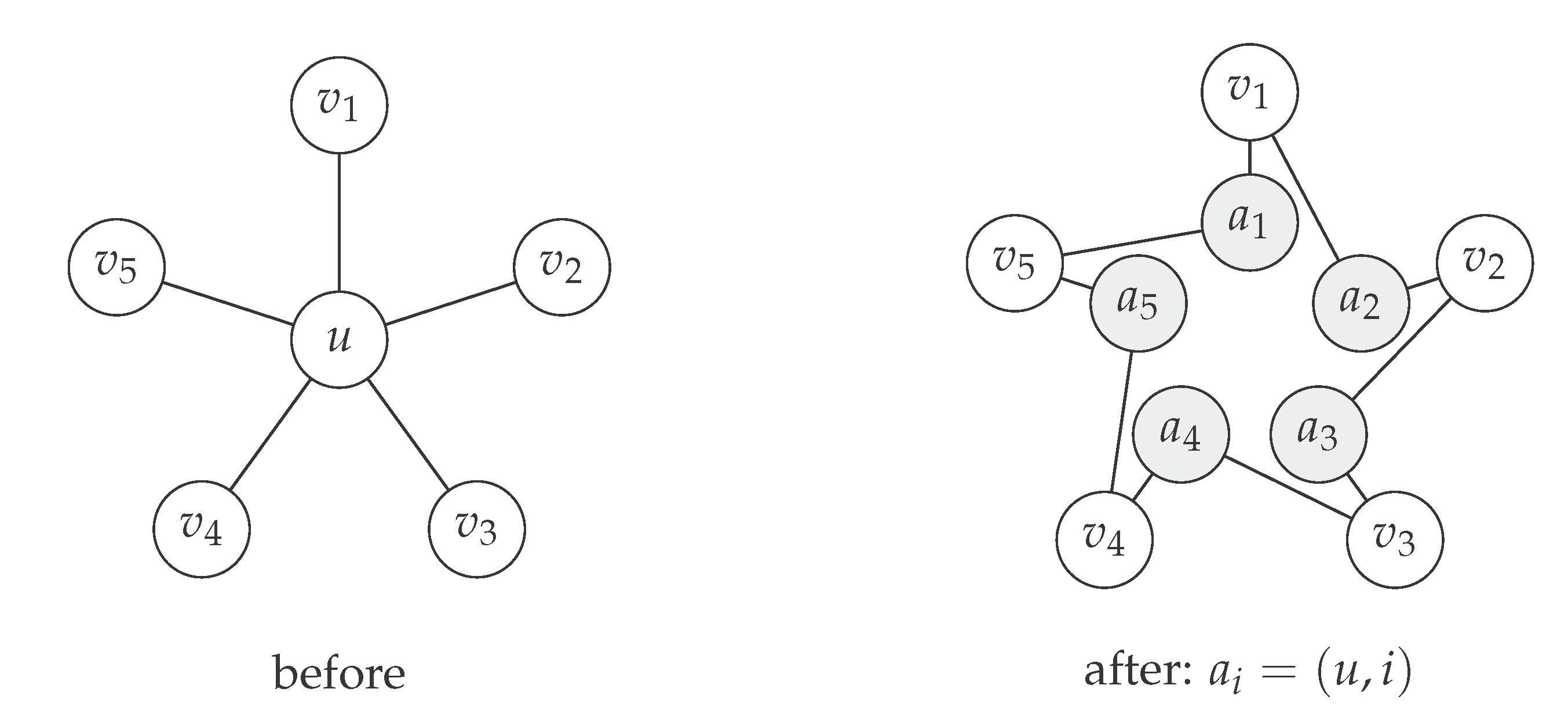
Table 1.
Code metadata for the siriaisa package used in this manuscript.
| Nr. | Code metadata description | Metadata |
|---|---|---|
| C1 | Current code version | v0.0.4 |
| C2 | Permanent link to code repository | https://github.com/frankvegadelgado/mids |
| C3 | Package name | siriaisa |
| C4 | Legal Code License | MIT License |
| C5 | Code versioning system used | git |
| C6 | Languages, tools, and services used | Python ≥ 3.12, NetworkX, NumPy, SciPy |
| C7 | Main entry points | iris, batch_iris, test_iris |
Table 2.
Family-specific approximation constants. Bounded-degree families obtain the constant from the maximal-set bound; rigid families obtain the constant 1 from exact recovery. No single constant covers all families, in agreement with Irving’s inapproximability theorem.
Table 2.
Family-specific approximation constants. Bounded-degree families obtain the constant from the maximal-set bound; rigid families obtain the constant 1 from exact recovery. No single constant covers all families, in agreement with Irving’s inapproximability theorem.
| Family | Optimum | Siriaisa constant | Reason |
|---|---|---|---|
| Path | 2 | , Cor. 1 | |
| Cycle | 2 | , Cor. 1 | |
| Ladder | 3 | , Cor. 1 | |
| Grid | 4 | , Cor. 1 | |
| r-regular | r | , Cor. 1 | |
| Clique | 1 | 1 | every MIS is one vertex, Prop. 1 |
| Star | 1 | 1 | LP/domination-power + one-add, Prop. 1 |
| Complete bipartite | 1 | smaller side selected, Prop. 1 | |
| Crown ( minus matching) | 2 | 1 | seed-pair recovery, Prop. 1 |
| Double star | 1 | centre-first + one-add, Prop. 1 | |
| Lollipop – | (typ.) | c | , Cor. 1 (opt. observed) |
Table 4.
car suite results over instances. “Guarantee” is the family constant proved in Section 7: the degree bound for bounded and random classes and exactly 1 for the rigid classes. Every family stays within its guarantee, and all thirteen families other than r-regular and Erdos–Rényi were solved exactly on every instance.
Table 4.
car suite results over instances. “Guarantee” is the family constant proved in Section 7: the degree bound for bounded and random classes and exactly 1 for the rigid classes. Every family stays within its guarantee, and all thirteen families other than r-regular and Erdos–Rényi were solved exactly on every instance.
| Family | Class | Instances | Mean ratio | Max ratio | Guarantee | Violations |
|---|---|---|---|---|---|---|
| Path | bounded | 667 | 1.0000 | 1.0000 | 0 | |
| Cycle | bounded | 667 | 1.0000 | 1.0000 | 0 | |
| Ladder | bounded | 667 | 1.0000 | 1.0000 | 0 | |
| Grid | bounded | 667 | 1.0000 | 1.0000 | 0 | |
| r-regular | bounded | 667 | 1.0029 | 1.2000 | 0 | |
| Balanced tree | bounded | 667 | 1.0000 | 1.0000 | 0 | |
| Lollipop – | bounded | 667 | 1.0000 | 1.0000 | 0 | |
| Clique | rigid | 667 | 1.0000 | 1.0000 | 0 | |
| Star | rigid | 667 | 1.0000 | 1.0000 | 0 | |
| Complete bipartite | rigid | 667 | 1.0000 | 1.0000 | 0 | |
| Crown | rigid | 666 | 1.0000 | 1.0000 | 0 | |
| Double star | rigid | 666 | 1.0000 | 1.0000 | 0 | |
| Erdos–Rényi | random | 666 | 1.0002 | 1.1429 | 0 | |
| Barabási–Albert | random | 666 | 1.0000 | 1.0000 | 0 | |
| Random tree | random | 666 | 1.0000 | 1.0000 | 0 | |
| All | — | 10000 | 1.0002 | 1.2000 | — | 0 |
Table 5.
The 15 non-optimal instances in the car suite, grouped by exact ratio. All are sparse regular or Erdos–Rényi graphs, and every one is within its maximal-set degree bound.
Table 5.
The 15 non-optimal instances in the car suite, grouped by exact ratio. All are sparse regular or Erdos–Rényi graphs, and every one is within its maximal-set degree bound.
| Exact ratio | Class | # instances | Typical |
|---|---|---|---|
| 3-regular | 4 | ||
| 3-regular | 2 | ||
| regular (), Erdos–Rényi () | 6 | ||
| 5-regular | 2 | ||
| 5-regular | 1 |
Disclaimer/Publisher’s Note: The statements, opinions and data contained in all publications are solely those of the individual author(s) and contributor(s) and not of MDPI and/or the editor(s). MDPI and/or the editor(s) disclaim responsibility for any injury to people or property resulting from any ideas, methods, instructions or products referred to in the content. |
© 2026 by the authors. Licensee MDPI, Basel, Switzerland. This article is an open access article distributed under the terms and conditions of the Creative Commons Attribution (CC BY) license (http://creativecommons.org/licenses/by/4.0/).
Copyright: This open access article is published under a Creative Commons CC BY 4.0 license, which permit the free download, distribution, and reuse, provided that the author and preprint are cited in any reuse.