

Submitted:
05 June 2026
Posted:
08 June 2026
You are already at the latest version
Abstract
The growing use of RISC-V processors in real-time embedded systems has increased the need for evaluation methods that can characterize timing behavior under scheduler-driven workloads. While existing simulation environments provide extensive support for architectural exploration and functional validation, they are not primarily designed for controlled timing-scalability studies across large configuration spaces. This paper presents nSim-RV, a configurable RISC-V simulation and orchestration framework developed for reproducible evaluation of timing behavior under increasing workload density. The framework combines automated campaign generation, structured dataset aggregation, validation procedures, and timing-oriented analysis within a unified workflow. The evaluation includes CoreMark, Dhrystone, and synthetic RT-Control workloads, task counts ranging from 2 to 32 concurrent tasks, observation windows from 50k to 1M cycles, cache-disabled and cache-enabled configurations, and both 4-stage and 5-stage pipeline organizations. A comparative analysis is performed between a Standard shared-pipeline execution model and an nMPRA-inspired preserved-context execution mode across 864 validated pipeline-specific configurations. Under cache-disabled conditions, response-time variability, execution jitter, and deadline miss ratio all increase monotonically with task count for both execution modes, with the most pronounced growth observed beyond N = 8 concurrent tasks. Preserved-context execution reduces switching-induced disturbance and delays the onset of saturation-phase behavior across the majority of evaluated trajectories, with the clearest benefit appearing in Dhrystone and RT-Control workloads at intermediate to high task counts.
Keywords:
RISC-V
; real-time systems
; timing analysis
; timing predictability
; context switching
; scheduling
; scalability analysis
; simulation framework
; execution jitter
; nMPRA
1. Introduction
In cyber-physical and industrial control systems, temporal predictability is often prioritized over peak instruction throughput. For these environments, the reliability of a processor is defined by its capacity to minimize task response-time variations, bound activation jitter, and consistently meet deadlines despite frequent preemptions. As RISC-V microcontrollers increasingly target these real-time domains, evaluating their ability to sustain execution continuity under mounting task concurrency has become a critical research challenge.
Historically, the RISC-V ecosystem has benefited from robust simulation and virtual-platform tools. Frameworks such as gem5 [1], FireSim [2], and GVSoC [3] provide comprehensive infrastructures for full-system execution, hardware/software co-design, and deep architectural exploration. However, these tools are not inherently optimized for the methodological demands of scheduler-aware timing scalability. Assessing how temporal behavior deteriorates as workload density grows requires more than just cycle-accurate modeling; it demands strict configuration control, automated scenario generation, and deterministic workload orchestration across massive design spaces. Without such a workflow, distinguishing genuine microarchitectural benefits from mere scheduling artifacts or workload inconsistencies becomes highly problematic.
This methodological gap is particularly evident when analyzing hardware-assisted scheduling mechanisms. In conventional shared-pipeline processors, preemptions forcefully flush in-flight instructions, forcing the system to incur a substantial recovery penalty before useful execution resumes. Previous work on predictable processor design has shown that architectural scheduling support can improve temporal isolation in mixed-criticality systems [4], while recent RISC-V studies have highlighted the critical impact of interrupt latency and context-switch overhead [5,6,7]. To counter this disruption, preserved-context execution models, such as the n-Multiple Pipeline Register Architecture (nMPRA) and its associated Hardware Scheduler Engine (nHSE) [8,9], replicate pipeline registers to retain task-specific architectural states across context switches. Quantifying the real-time advantages of such mechanisms requires subjecting both standard and preserved-context pipelines to identical, highly controlled scheduler pressure.
To facilitate this level of rigorous timing analysis, this paper presents nSim-RV: an automated RISC-V simulation and orchestration framework explicitly tailored for reproducible scalability studies. Rather than functioning as a full-system virtual platform, nSim-RV isolates and measures the temporal degradation induced by scheduler activity. The framework automates campaign execution, dataset aggregation, and metric extraction, ensuring methodological consistency across hundreds of configurations. This structure closely follows the broader requirements for reproducible experimental research and portable experiment workflows [10,11].
nSim-RV is applied here to contrast a conventional Standard shared-pipeline mode against an nMPRA-inspired preserved-context execution mode, tracing how execution continuity affects timing variability and deadline pressure as concurrent task counts scale from 2 to 32.
The main contributions of this work are as follows:
1. Scientific Contribution: nSim-RV, a configurable RISC-V simulation framework dedicated to scheduler-aware timing evaluation under controlled real-time workloads, together with a reproducible timing-scalability evaluation methodology based on response-time variability, execution jitter, deadline miss ratio, switch-overhead pressure, and scalability-phase characterization.
2. Theoretical Contribution: Formalization of timing-scalability assessment through a multidimensional metric framework and an operational scalability-phase classifier that distinguishes stable, tipping, saturation, and collapse execution regions under increasing workload density.
3. Practical Contribution: An automated orchestration workflow supporting campaign generation, execution, duplicate validation, dataset construction, and aggregated timing analysis across pipeline organizations, cache configurations, execution modes, observation windows, and task counts.
4. Derivative Contribution: A validated dataset comprising 864 scheduler-controlled configurations and a reusable experimental workflow that can support future investigations involving RTOS integration, hardware-assisted scheduling concepts, timing prediction techniques, and extended RISC-V execution organizations.
nSim-RV targets scheduler-aware timing-scalability evaluation. Its focus is on how response-time variability, execution jitter, deadline miss ratio, switch-overhead pressure, and scalability-phase transitions change as workload density increases, rather than on maximizing throughput or reproducing hardware at cycle accuracy. Limitations of scope, including the absence of full RTOS integration, multicore modeling, and hardware-level validation, are discussed in Section 5.4.
2. Related Work
2.1. RISC-V Simulation and Virtual Platform Environments
The RISC-V ecosystem includes a broad range of simulation and virtual-platform tools developed for architectural exploration, functional validation, and system-level evaluation. gem5 remains one of the most widely used architectural simulators in academic research, providing configurable in-order and out-of-order processor models, coherent cache hierarchies, and multi-ISA support for detailed processor studies [1]. FireSim complements software-based simulation by enabling FPGA-accelerated, cycle-accurate simulation of complete RISC-V SoCs, supporting hardware/software co-exploration at high simulation speed [2]. GVSoC targets the embedded and IoT segment with a configurable, event-driven full-platform simulator for PULP-based RISC-V processors [3].
Recent tools have extended this landscape in several directions. Shahid et al. developed a validated gem5 model of the CVA6 RISC-V core and used it for machine-learning-assisted design-space exploration of microarchitectural configurations [12]. Tempel et al. addressed the link between formal ISA specification and simulator correctness by generating RISC-V instruction-set simulators from the Sail formal model [13]. Herdt et al. investigated the simulation speed-accuracy trade-off through runtime-switchable fidelity in a SystemC-based RISC-V virtual prototype [14]. Schlögl et al. extended virtual prototyping toward the RISC-V vector extension, enabling system-level evaluation of RVV workloads without requiring RTL implementation [15]. Qiu and Liu proposed a UVM-TLM co-simulation framework that combines functional verification and early performance evaluation of RISC-V cores within a single flow [16].
These platforms show the maturity and diversity of the RISC-V simulation ecosystem. Their main objectives, however, remain microarchitectural optimization, ISA validation, fidelity adaptation, verification, and full-system execution. None of these environments were designed for controlled scheduler-aware timing-scalability studies in which workload density is systematically varied while scheduling semantics remain identical across compared execution modes. This is the methodological space targeted by nSim-RV.
2.2. Timing-Predictable and Real-Time RISC-V Execution
Timing predictability is a central requirement of hard real-time systems. The survey by Wilhelm et al. established that architectural features such as caches, pipelines, and branch predictors make it difficult to compute safe and tight worst-case execution-time bounds, motivating both static analysis methods and predictable processor designs [17]. FlexPRET is a representative hardware response: it uses fine-grained thread interleaving with a hardware-managed schedule to provide temporal isolation between hard and soft real-time threads on a shared processor [4].
In the RISC-V domain, the performance gap between open ISA designs and mature proprietary real-time architectures has been studied in increasing detail. Balas and Benini profiled the CV32E40P core under FreeRTOS and identified interrupt latency and context-switch overhead as important limitations, reporting 25% context-switch reduction and 33% average interrupt-latency reduction through software optimization [5]. CV32RT extended this core with CLIC-based interrupt support and a FastIRQ mechanism, reducing interrupt latency to as little as six cycles and improving RTOS task context switching [6]. Scheck et al. approached the same bottleneck from the hardware/software co-design direction, introducing RTOSUnit, a configurable hardware unit that offloads context storage, loading, and task scheduling; their results report up to 76% reduction in mean context-switch latency and, in selected configurations, complete elimination of context-switch jitter [7].
Application-oriented studies further confirm the practical importance of timing behavior in RISC-V systems. Yoo and Choi benchmarked RISC-V real-time performance in an EtherCAT-based robotic control system, showing the practical relevance of RISC-V in control-oriented embedded applications [18]. Platzer and Puschner addressed predictability in data-parallel execution with Vicuna, a timing-predictable RISC-V vector coprocessor designed to support WCET-analyzable vector computation [19].
These works show that interrupt responsiveness, context-switch latency, and timing predictability remain active concerns in RISC-V real-time systems. nSim-RV does not optimize a specific core or RTOS implementation. Instead, it provides a controlled framework for evaluating how switch-related timing effects scale with workload density when alternative execution models are compared under identical scheduler and workload conditions.
2.3. Hardware-Assisted Scheduling and Preserved-Context Execution
A related line of work has explored hardware mechanisms for reducing the execution disruption caused by task switching. The nMPRA microarchitecture uses replicated pipeline-register resources to maintain task-specific execution state in hardware, allowing task switching without the conventional save/restore sequence [8]. The companion nHSE engine implements scheduling functions in hardware and supports policies such as fixed-priority, round-robin, and earliest-deadline-first scheduling [9]. Together, these architectures motivate preserved-context execution as a hardware-oriented strategy for improving real-time responsiveness.
Other RISC-V-compatible designs also address hardware-assisted context management. Zagan et al. implemented hardware real-time event management with RISC-V support for FPGA-based reconfigurable embedded systems [20]. Nurmi et al. introduced the HETI architecture, which integrates a stacked register file for selective hardware-accelerated context switching of high-priority interrupts, reducing retired instruction count by up to 26% and increasing sleep time by up to 21%, with a reported gate-count overhead of 1.2% for a representative HETI-4 instance [21].
The nMPRA-inspired execution mode in nSim-RV is grounded in this hardware-context-preservation literature. Within nSim-RV, it is modeled as an execution organization rather than as a cycle-accurate implementation of a specific processor. This allows the timing consequences of preserved execution state to be evaluated under the same workload, scheduler, and measurement conditions used for the Standard shared-pipeline mode.
2.4. Reproducible Experimental Workflows and Dataset-Oriented Evaluation
As simulation studies grow in configuration-space size, reproducing the exact experimental conditions becomes an important methodological requirement. Demchenko et al. proposed a structured workflow-management approach for experimental reproducibility, covering experiment description, workflow specification, execution environment management, and result validation [10]. Stubbe et al. formalized a related methodology for portable experiment workflows by separating experiment design, environment specification, execution control, and result analysis into composable stages [11].
Simulation reproducibility has also been addressed from broader methodological perspectives. Huang analyzed the distinction between reproducibility and replicability in simulation models, identifying issues such as model ambiguity, PRNG sensitivity, platform dependencies, and insufficient documentation [22]. Teijema et al. presented Makita, a workflow generator for large-scale reproducible simulation studies in the context of systematic-review text-labeling experiments; although its application domain differs from embedded systems, its configuration-driven orchestration principle is relevant to large simulation campaigns [23].
nSim-RV applies these workflow principles to scheduler-aware RISC-V timing evaluation. The framework separates design-space definition, campaign generation, simulation execution, result aggregation, duplicate detection, and metric analysis into distinct stages. This structure supports traceable dataset construction and makes large configuration matrices reproducible rather than dependent on manually executed simulation runs.
2.5. Positioning of nSim-RV
Table 1 positions nSim-RV relative to representative works from the simulation and evaluation landscape. The key distinction is native support for scheduler-aware timing-scalability evaluation: nSim-RV enforces identical scheduler semantics across compared execution modes and automatically generates experiment matrices, enabling timing-trend attribution under controlled task-density variation.
As shown in Table 1, nSim-RV is narrower in scope than general-purpose or full-system RISC-V simulators. Its distinction is not that such timing metrics are impossible in existing environments, but that scheduler-aware workload generation, campaign orchestration, dataset validation, and timing-scalability analysis are provided as native parts of the evaluation workflow. Its role is to preserve identical scheduler and workload semantics across configurable execution models while automating campaign generation, dataset aggregation, validation, and timing analysis. This allows nSim-RV to complement existing simulation environments by focusing on scheduler-aware timing behavior rather than broader architectural or full-system evaluation.
3. Materials and Methods
3.1. nSim-RV Timing-Oriented Framework
The experimental infrastructure used is built around nSim-RV, a configurable RISC-V simulation framework for timing evaluation under real-time workloads. The framework is designed to execute controlled experiments in which identical workload and scheduling conditions are preserved across different execution organizations. Its purpose is not to replace full-system architectural simulators, but to provide a compact and reproducible environment for observing timing variability, scheduler-induced execution effects, workload-density behavior, and deadline-oriented trends under periodic real-time workloads. nSim-RV advances execution in cycle steps and combines instruction-level execution control with explicit pipeline-state modeling.
This execution model allows the same experimental workload to be evaluated under different execution organizations while preserving a common scheduler, timing model, and instrumentation interface. This allows the same experimental workload to be evaluated under different execution organizations while preserving a common scheduler, timing model, and instrumentation interface. The framework compares conventional Standard shared-pipeline execution with an nMPRA-inspired preserved-context execution mode. The nMPRA and nHSE concepts provide the architectural background for preserved execution context and hardware-supported scheduling in real-time systems [8,9]. In nSim-RV, these concepts are modeled at the execution-organization level and are used as a controlled comparison case, rather than as a cycle-accurate reproduction of a specific hardware implementation.
At simulation level, the Standard mode uses a shared in-flight pipeline state across tasks. When a task switch occurs, the currently active pipeline context is interrupted, and useful pipeline progress must be rebuilt before the resumed task can continue. In the nMPRA-inspired mode, task-specific architectural state and pipeline-related execution state are maintained per context, including the program counter, general-purpose register state, and modeled pipeline-stage registers. A resumed task can therefore continue from its preserved state rather than rebuilding execution progress in a shared pipeline. This abstraction captures the timing effect of preserved context on task resumption while avoiding claims of cycle-accurate equivalence to a specific hardware implementation.
The framework also supports configurable pipeline depth. The 4-stage configuration merges execution and memory access into a combined EX/MEM stage followed by writeback, whereas the 5-stage configuration follows the conventional IF, ID, EX, MEM, and WB organization. The 5-stage configuration serves as the primary reference, while the 4-stage configuration replicates the full experimental matrix to verify that timing-scalability trends are not specific to a single pipeline depth.
A central methodological requirement in nSim-RV is that scheduling conditions remain consistent across configurations. Task release, period, deadline, budget, and completion information are tracked through the same timing model, while context-switch and execution-progress indicators are collected through a common instrumentation interface. This makes it possible to compare execution modes and pipeline configurations without introducing additional variability caused by different scheduler policies or workload definitions.
The scheduler used in the evaluation is a fixed-priority preemptive scheduler. Each task is assigned a static priority in the workload configuration, and released jobs become eligible according to their configured period and release offset. At each scheduling decision point, the ready job with the highest priority is selected for execution; if multiple ready jobs share the same priority, a deterministic task-identifier order is used as tie-breaking. A newly released higher-priority job may preempt the currently executing task. The same scheduler policy, priority assignment, release model, execution budgets, and deadline definitions are preserved across Standard and nMPRA-inspired execution modes.
Figure 1 summarizes the nSim-RV evaluation workflow used in this study, from reproducible configuration inputs to automated campaign execution, dataset aggregation, and timing-scalability analysis.
The framework records both scheduler-level and execution-level timing information. At the scheduler level, it tracks task activations, completed jobs, response-time behavior, deadline misses, and context-switch activity. At the execution level, it records pipeline-related timing statistics and progress indicators needed to characterize workload-density effects. These measurements support the scalability-oriented metrics used, including response-time variability, execution jitter, deadline miss ratio, context-switch and switch-overhead indicators, and phase-oriented scalability behavior.
3.2. Experimental Orchestration Workflow
The experimental workflow implemented around nSim-RV is organized as a configuration-driven process. Each simulation run is generated from an explicit set of workload, timing, and execution parameters, including workload class, task count, observation window, execution mode, pipeline organization, and cache setting. This structure follows established reproducibility practices, where explicit configuration metadata and repeatable execution procedures support consistent evaluation across large design spaces [10,11].
The first stage defines the experimental design matrix. This matrix combines the selected workload classes, task-count settings, observation-window durations, execution modes, pipeline configurations, and cache modes. Each generated configuration therefore represents a unique experimental point that can be reproduced, inspected, or rerun under the same input conditions. By explicitly encoding these dimensions, the workflow reduces the risk of implicit configuration changes between simulation runs.
The second stage performs automated campaign generation and execution. The orchestration scripts expand the design matrix into executable simulation scenarios, instantiate the corresponding nSim-RV configuration files, launch the simulator, and store the raw outputs using consistent naming and metadata conventions. This automated process limits manual intervention and ensures consistent execution across all evaluated configurations. Table 2 summarizes the main stages of the nSim-RV orchestration process and the artifacts generated at each stage.
During each run, nSim-RV executes the selected workload under the configured execution model and scheduler-controlled task model. The simulator records both raw execution outputs and structured timing information, including task-level response behavior, completed jobs, deadline-related data, context-switch activity, and execution-progress indicators. The same output structure is used across workloads, execution modes, and pipeline configurations, which simplifies aggregation and supports consistent comparison.
After simulation execution, the aggregation pipeline merges the per-run outputs into CSV and JSON datasets. Each row is associated with explicit metadata describing the corresponding experimental configuration. The aggregation process uses a composite configuration key based on pipeline stage count, execution mode, workload, task count, observation window, and cache mode. This key is used to identify duplicate configurations and retain a single authoritative result for each unique configuration.
The validated dataset is then used as input for timing-scalability analysis. The analysis stage derives the metrics used, including response-time variability, execution jitter, deadline miss ratio, context-switch demand, modeled switch-overhead pressure, average IPC, and scalability-phase behavior. Average IPC is retained as a secondary throughput reference for interpreting degradation trends under increasing task-count pressure, while the primary interpretation remains focused on timing variability, deadline pressure, and scheduler-induced execution effects.
This separation of concerns, design-space generation, simulation execution, aggregation, validation, and metric extraction as distinct stages, is what makes the methodology portable to alternative execution models, scheduling policies, or workload classes without re-engineering the orchestration layer.
3.3. Workload and Scalability Configuration
The evaluation configuration is designed to expose timing behavior under increasing workload density while preserving comparability across execution modes and pipeline organizations. For this reason, the experimental space combines workload diversity, task-count scaling, observation-window scaling, execution-mode variation, pipeline-depth variation, and cache configuration.
Three workload classes are used in the evaluation. CoreMark is included as a compute-oriented embedded benchmark designed to provide a compact and portable measure of processor execution capability [24]. Dhrystone is included as a classical integer benchmark with branch and control-flow characteristics that remain useful for lightweight embedded evaluation contexts [25]. In addition, RT-Control is used as a synthetic control-oriented workload designed to expose scheduler-induced timing variability under increasing task-count pressure. RT-Control is not treated as a standardized benchmark; instead, it provides controlled periodic task sets with reproducible activations, execution budgets, and deadline-pressure conditions.
RT-Control uses two deterministic generation paths, depending on the experiment type. The first path supports the unified scalability sweeps and builds task sets by selecting the first N templates from a fixed pool. This path supports the evaluated scalability counts, including N = 2, and maps the generated tasks to the RT-Control workload program. For example, the N = 2 configuration is deterministically generated from the first two templates of the pool: Task 0 uses priority 1, WCET 20000 cycles, period 40000 cycles, and next release 0, while Task 1 uses priority 2, WCET 50 cycles, period 1000 cycles, and next release 0.
The second path supports the targeted C1–C4 validation scenarios. These scenarios start from explicit four-task JSON configurations representing baseline, preemption-stress, near-overload, and tight-deadline cases. In this path, scaling below four tasks is not supported; larger task sets are generated by replicating the four-task base configuration. During replication, periods and implicit deadlines are scaled by the replication factor, execution budgets are preserved, and release offsets are interleaved deterministically. Nominal scenarios use implicit deadlines equal to task periods, whereas tight-deadline scenarios explicitly define constrained deadlines.
Table 3 summarizes the two RT-Control workload-generation paths used in the evaluation. This distinction is important for reproducibility because task counts below four are generated only by the unified template-pool mechanism and not by the four-task scenario replication mechanism.
For reproducibility, the complete RT-Control template pool and the generated scenario files are treated as part of the experimental artifacts. The manuscript reports the workload-generation mechanism and a representative N = 2 configuration, while the full set of task templates, generated JSON configurations, workload program mappings, aggregation scripts, and phase-classification scripts are provided as supporting artifacts according to the Data Availability Statement.
Across both generation paths, the same scheduler semantics and task definitions are preserved when comparing Standard and nMPRA-inspired execution modes. This ensures that differences observed between the execution organizations are not caused by different workload definitions within the same evaluated configuration. The unified scalability sweep is used to support task-count scalability analysis, while the C1–C4 scenario path provides targeted validation cases for baseline, preemption-stress, near-overload, and tight-deadline behavior.
Task-count scaling uses selected values from N = 2 to N = 32 concurrent tasks, depending on the generation path and the available validated configurations. The selected task-count set covers low-density, intermediate, saturation-oriented, and high-pressure workload regions without assuming continuous coverage of every possible task count. This design allows the evaluation to observe how response-time variability, execution jitter, deadline miss behavior, switch-overhead pressure, and throughput retention evolve as the number of scheduler-managed execution contexts increases.
Observation-window scaling is performed using fixed execution intervals of 50k, 100k, 500k, and 1M simulation cycles. The use of fixed observation windows provides a common basis for comparing configurations under identical simulation budgets. Shorter windows capture bounded early run timing behavior, whereas longer windows expose sustained scheduler-pressure effects and phase transitions that may not be visible in compact runs. The 50k and 100k windows are therefore interpreted as compact observation intervals rather than as steady-state estimates.
The evaluated modes include Standard shared-pipeline execution and nMPRA-inspired preserved-context execution. Both modes are evaluated under identical scheduler and workload conditions, so that observed timing differences can be attributed to the execution mode rather than to scheduling policy or workload structure. The analysis therefore focuses on how timing variability and deadline-oriented behavior evolve under identical workload and scheduling conditions, rather than on isolated microarchitectural recovery mechanisms.
The evaluation includes both 5-stage and 4-stage pipeline organizations. The 5-stage configuration is used as the reference pipeline organization, while the 4-stage configuration was evaluated through a complete parity matrix that mirrors the same workload, task-count, observation-window, cache, and execution-mode structure. In the results, both matrices are reported together for the main cache-disabled timing analysis, while the interpretation remains focused on timing behavior rather than pipeline-depth optimization. Table 4 summarizes the main experimental dimensions used in the evaluation.
The resulting configuration space supports a timing-scalability analysis centered on temporal stability and scheduler pressure. This configuration strategy provides the basis for the metrics defined in the next section.
3.4. Timing-Oriented Metrics
The evaluation focuses on metrics that describe how execution behavior evolves under increasing task-count pressure. The selected metrics capture temporal variability, execution jitter, deadline pressure, context-switch activity, modeled switch-overhead pressure, and scalability-phase transitions. Average IPC is retained as a secondary throughput reference, since the main objective of this study is not peak instruction retirement, but timing stability under scalable real-time workloads.
For each completed task job, response time is measured as the interval between job release and job completion. For job k of task i, response time is defined as:
where R_(i,k) is the response time of job k of task i, t_(i,k)^release is the release cycle, and t_(i,k)^finish is the completion cycle.
Response-time variability is represented by the spread between the maximum and minimum observed response times for a given task within the evaluated interval:
where R_i^max and R_i^min are the maximum and minimum observed response times for task i. A lower response-time spread indicates more stable task completion behavior, whereas a larger spread reflects increased timing variability.
Execution jitter quantifies activation-level timing variation across repeated scheduler-controlled task releases. Unlike response-time spread, which captures completion-time dispersion, jitter is defined here as an activation-related timing-spread indicator:
where A_i^max and A_i^min denote the maximum and minimum observed activation-to-resumption timing values for task i under the same configuration, measured from the cycle at which a released task becomes scheduler-eligible to the cycle at which it resumes useful modeled execution. This separates jitter from response-time variability: response-time variability describes the spread of job completion behavior, while jitter emphasizes activation-to-activation timing variation induced by scheduler activity and workload-density pressure.
Deadline behavior is evaluated using the deadline miss ratio. This metric normalizes the number of deadline violations by the number of evaluated jobs in the corresponding simulation interval:
where, N_miss is the number of jobs that miss their configured deadline and N_jobs is the total number of evaluated jobs in the corresponding simulation interval. The deadline miss ratio provides a configuration-level view of deadline pressure and enables comparison across task-count settings, workloads, and observation windows.
Context-switch demand is used as a scheduler-level validation indicator. It captures the frequency of context-switch requests relative to the simulated execution interval:
where N_switch is the number of observed task-to-task context-switch events and C_total is the total number of simulated cycles in the observation window. This metric is used to verify that matched Standard and nMPRA-inspired configurations are subjected to comparable scheduler demand.
Switch-overhead pressure is used as a modeled execution-level indicator. It measures the fraction of the observation window accounted for by explicit context-switch overhead cycles in the simulator:
where C_switch is the number of cycles explicitly accounted as context-switch overhead by the simulator, and C_total is the total number of simulated cycles in the observation window.
In Standard mode, this pressure reflects the pipeline-depth-dependent penalty associated with task-to-task switching in the shared-pipeline organization. In the simulator, each Standard-mode task-to-task switch adds a modeled flush-and-recovery penalty of four cycles for the 5-stage organization and three cycles for the 4-stage organization. These constants represent the modeled recovery interval required before useful execution resumes after disrupting the shared in-flight pipeline state. In the nMPRA-inspired mode, this explicit modeled penalty is not applied because task-specific pipeline-related state is preserved across activations. Switch-overhead pressure should therefore be interpreted as a modeled execution-organization effect, not as the number of scheduler switch requests or as a hardware measurement of a specific implementation.
Average IPC is retained as a secondary throughput indicator. It is computed directly from the number of retired instructions and the total number of simulated cycles:
where N_retired is the number of retired instructions and C_total is the number of simulated cycles in the observation window.
Average IPC provides a useful-work reference for interpreting throughput retention and degradation under increasing task-count pressure. However, the timing-oriented interpretation remains centered on response-time variability, execution jitter, deadline miss ratio, context-switch demand, and switch-overhead pressure. Table 5 summarizes the metrics used and their role in the timing-scalability analysis.
Scalability-phase characterization summarizes timing behavior progression across the task-count axis. Phase labels are assigned using an operational rule applied independently to each trajectory: a unique combination of workload, execution mode, pipeline stage count, cache mode, and observation window. A trajectory is defined as a unique combination of workload, execution mode, pipeline stage count, cache mode, and observation window. For each trajectory, the maximum observed IPC is first identified, and each task-count configuration is then evaluated relative to this trajectory-specific peak.
The phase classifier uses IPC only to locate the empirical throughput peak and to detect post-peak degradation. The timing interpretation of the phases is based on the combined behavior of switch-overhead pressure and deadline-miss behavior, together with the response-time and jitter trends analyzed in the results. This avoids assigning phases from fixed task-count intervals and makes the classification reproducible from the validated dataset.
For a configuration with IPC value IPC(N), the relative peak ratio is defined as:
The phase rules are applied in descending severity order. A configuration is classified as collapse if IPC_peak_ratio(N) < 0.90 or if the deadline miss ratio exceeds 0.05. If the collapse condition is not met, the configuration is classified as saturation when switch-overhead pressure is at least 2.5% or deadline miss ratio is at least 0.02. If neither collapse nor saturation is met, the configuration is classified as tipping when switch-overhead pressure is at least 1.0% or deadline miss ratio is at least 0.005. All remaining configurations are classified as stable.
The selected thresholds were chosen as internal operational cut points after inspecting the distribution of switch-overhead pressure, deadline miss ratio, and post-peak IPC degradation in the validated dataset. They are intended to distinguish low-overhead operation, first observable timing stress, persistent deadline or switch-overhead pressure, and severe post-peak degradation. They should therefore be interpreted as reproducible dataset-level criteria rather than as universal real-time schedulability thresholds. Table 6 summarizes the resulting phase-classification rule.
Microarchitectural continuity metrics such as Useful Work Ratio, Execution Disruption Ratio, and Resume Latency are excluded because their cross-mode comparability depends on implementation-level pipeline details outside the scope of nSim-RV’s execution-mode abstraction.
3.5. Dataset Aggregation and Validation
The experimental campaigns generate multiple per-run outputs that must be aggregated before comparative timing analysis can be performed. For consistency and reproducibility, each result is associated with explicit metadata describing the pipeline stage count, execution mode, workload, task count, observation window, cache mode, and scenario label where applicable. For a fixed configuration, nSim-RV produces deterministic execution behavior and identical metric values across repeated runs; therefore, the study reports configuration-level deterministic outcomes rather than statistical confidence intervals.
The journal-analysis dataset is organized around two pipeline-specific matrices. The primary 5-stage scalability matrix contains 432 unique configurations. To provide a pipeline-depth parity evaluation, a complete 4-stage matrix was generated using the same workload, task-count, observation-window, cache, and execution-mode structure, resulting in an additional 432 validated configurations. The combined evaluation therefore includes 864 validated pipeline-specific configurations. The 4-stage matrix mirrors the 5-stage configuration space and is used to assess whether the workflow and main timing-scalability trends remain consistent across pipeline depth.
The aggregation process also preserves row-level analysis outputs used by the figure-generation and phase-classification scripts. In the primary journal-analysis files, multiple rows may correspond to derived or expanded analysis views of the same unique configuration. For this reason, the manuscript uses validated unique configurations as the main dataset-size indicator; additional analysis rows are retained only for plotting, filtering, and phase characterization. Table 7 summarizes the composition of the aggregated dataset and the validation rules applied during dataset construction.
To prevent repeated experimental configurations, duplicate detection uses a composite key composed of pipeline stage count, execution mode, workload, task count, observation window, cache mode, and scenario label where applicable. When duplicate entries are encountered during aggregation, a single authoritative result is retained for the corresponding unique configuration.
The validated dataset provides a unified basis for the analyses presented in this study. Response-time variability, execution jitter, deadline miss ratio, context-switch demand, modeled switch-overhead pressure, average IPC, and scalability-phase labels are derived from consistently structured data sources. For the operational scalability-phase classifier, both pipeline stage count and cache mode are included in the trajectory key so that pipeline-depth and cache configurations are evaluated relative to their own trajectory-specific IPC peaks.
By preserving configuration metadata, applying composite-key duplicate detection, and generating structured CSV/JSON outputs, the aggregation pipeline ensures that each row in the analysis dataset can be traced to its originating simulation configuration, a prerequisite for the figure-generation and phase-classification scripts provided in the reproducibility package.
4. Comparative Timing-Scalability Evaluation
In the following cache-disabled timing figures, CoreMark and Dhrystone may show overlapping scheduler-level trajectories because both workloads use the same deterministic periodic task templates and fixed-latency memory model. Their instruction-level behavior remains distinct, as reflected by the IPC results.
4.1. Baseline Throughput Scaling
Figure 2 presents the average IPC obtained under task-count scaling for the cache-disabled configurations. The results are reported for the CoreMark, Dhrystone, and RT-Control workloads using both the Standard and nMPRA-inspired execution modes in the 5-stage and 4-stage pipeline organizations.
Average IPC increases with task count and reaches its highest values near N = 16 tasks for most cache-disabled configurations (Figure 2). This trend is visible across all evaluated workloads and both pipeline organizations. Beyond the peak region, throughput progressively declines as increasing scheduler activity, more frequent task releases, and deadline-related preemptions consume a larger fraction of the available execution cycles. Although the exact peak location varies slightly for some trajectories, N = 16 represents the most common operating point at which useful execution throughput is maximized.
The advantage of preserved-context execution is particularly visible in Dhrystone and RT-Control. In the 5-stage organization, the nMPRA-inspired mode reaches peak IPC values of 0.666 and 0.877, compared with 0.427 and 0.706 for the corresponding Standard configurations, representing improvements of approximately 56% and 24%, respectively. CoreMark exhibits a smaller but still consistent benefit, with peak IPC increasing from 0.710 to 0.761. These results indicate that preserving task-specific execution state reduces the throughput loss associated with repeated pipeline disruption and recovery during scheduler-driven task switching.
Pipeline depth affects Standard-mode throughput more strongly than preserved-context throughput. The largest differences appear in Dhrystone and RT-Control, where the 5-stage Standard configuration experiences a more pronounced throughput decline after the peak region than its nMPRA-inspired counterpart. In contrast, the 4-stage organization exhibits a smaller separation between the execution modes, which is consistent with the reduced flush-and-rebuild penalty associated with the shorter pipeline. Nevertheless, both organizations eventually experience throughput degradation at high task counts, confirming that context preservation delays, but does not eliminate, the scalability limits imposed by dense scheduler-driven workloads.
4.2. Response-Time Variability Analysis
Response-time spread, normalized to the observation window, remains low up to intermediate task counts and increases sharply once scheduler pressure becomes dominant (Figure 3). For the 5-stage Standard mode, spread reaches 0.238 of the observation window at N = 16 tasks in CoreMark and Dhrystone, compared with 0.039 for the corresponding nMPRA-inspired configuration, representing a reduction of approximately 83.8%. At N ≤ 12, both modes maintain spread below 0.033 of the observation window, indicating that scheduler demand at low and intermediate task counts is not sufficient to generate large timing dispersion.
The mechanism differs between modes. In Standard execution, each task switch interrupts the shared in-flight pipeline state, and the resuming task must rebuild execution progress before contributing useful work. At N = 16, the 5-stage Standard configuration reaches 12,218 switches per 1M cycles in CoreMark and Dhrystone, while the cumulative switch overhead accounts for 4.887% of the observation window. This recovery cost amplifies response-time dispersion because jobs completed under different preemption patterns accumulate different amounts of rebuild latency within the same observation interval.
In the nMPRA-inspired mode, task-specific pipeline-related state is retained across activations, so resumed tasks can continue execution without the same shared-pipeline rebuild penalty. This explains the lower spread observed around the peak-throughput region. However, the residual spread increase at higher task counts, especially beyond N = 20, shows that context preservation does not remove release-density effects or deadline-pressure accumulation. At N = 32, both execution modes enter a high-pressure region, and response-time spread becomes dominated by workload density rather than by switch recovery alone.
CoreMark and Dhrystone produce overlapping response-time trajectories under cache-disabled conditions, as expected from their shared scheduler-level timing templates; their distinct IPC values in Figure 2 confirm that instruction-level behavior remains different.
4.3. Execution Jitter Analysis
Activation-level jitter, normalized to the observation window, remains limited to low and intermediate task counts but rises sharply beyond N = 16 tasks in Standard mode (Figure 4). For the 5-stage RT-Control configuration, jitter reaches approximately 33.0% of the observation window at N = 32, whereas the corresponding nMPRA-inspired configuration reaches 12.1%, representing a reduction of approximately 63%. Below N = 12, both execution modes generally remain below 3.5% of the observation window, indicating that activation-to-activation regularity is preserved when scheduler pressure remains moderate.
Jitter in Standard mode is driven by preemption-induced pipeline flushes that vary the cycle at which each task resumes useful execution. Because the recovery cost is affected by pipeline depth, the 5-stage Standard configuration produces approximately 39.8% higher jitter than the 4-stage Standard configuration at N = 32. In contrast, the 5-stage and 4-stage nMPRA-inspired trajectories remain substantially closer to each other than the corresponding Standard-mode trajectories, indicating that preserved context reduces the sensitivity of activation-level timing regularity to pipeline depth.
The RT-Control workload shows the steepest jitter growth after N = 16, increasing by approximately 1.65 percentage points per additional task up to N = 32. The RT-Control workload combines tighter deadline constraints with higher preemption pressure than CoreMark and Dhrystone, which accounts for its steeper jitter increase.
4.4. Deadline Miss Ratio Analysis
Deadline miss ratio remains negligible at low task counts across all evaluated workloads and execution modes (Figure 5). For the 5-stage RT-Control configuration, the Standard mode reaches a maximum deadline miss ratio of approximately 3.75% at N = 32, whereas the corresponding nMPRA-inspired configuration reaches 2.22%, representing a reduction of approximately 40.8%. The divergence becomes visible beyond N = 16 tasks, where increasing scheduler pressure and execution interference begin to consume a measurable fraction of the available timing budget.
Figure 6B provides the corresponding switch-overhead pressure profile for interpreting this deadline-miss growth. In Standard execution, each task switch interrupts the shared pipeline state and introduces a pipeline-depth-dependent recovery interval before useful work can resume. As task count increases, the accumulated recovery cost reduces the effective execution budget available between release and deadline, directly increasing the probability of deadline violations.
Preserved-context execution does not apply this modeled source of execution disruption within the evaluated execution model. Consequently, resumed tasks can continue execution without paying the same recovery penalty observed in the Standard mode. The resulting preservation of useful execution cycles delays the growth of deadline miss ratio and shifts the onset of deadline-pressure effects toward higher task counts.
The largest separation between execution modes is observed in the RT-Control workload, which combines tighter timing constraints with higher preemption activity. At N = 32, the 5-stage Standard configuration reaches a deadline miss ratio of 3.75%, compared with 2.22% for the corresponding nMPRA-inspired configuration. In contrast, CoreMark and Dhrystone exhibit nearly identical deadline-miss trajectories, which is expected because both benchmarks share the same deterministic scheduler-level timing templates in the cache-disabled experiments.
4.5. Switch-Overhead Pressure Analysis
The previous metrics describe the visible timing effects of workload-density scaling. To relate these effects to the execution model, this section analyzes modeled switch-overhead pressure introduced by task-to-task context switches. This metric differs from scheduler demand: scheduler demand reflects how often the scheduler requests context switches, whereas switch-overhead pressure captures the fraction of the observation window consumed by the modeled switch penalty.
In the Standard shared-pipeline mode, switch-overhead pressure increases as task count grows. This follows from the larger number of task activations and preemptions generated by denser workload configurations. Because Standard mode uses a shared in-flight pipeline state, task-to-task switches introduce an explicit modeled penalty associated with interrupting and rebuilding useful pipeline progress. The effect is stronger in the 5-stage configuration than in the 4-stage configuration because the modeled Standard-mode penalty is pipeline-depth dependent.
In the nMPRA-inspired preserved-context mode, explicit switch-overhead pressure remains zero by design. This does not mean that scheduler demand disappears; the scheduler still activates and switches tasks according to the same workload definitions. Rather, the preserved-context model does not apply the same explicit flush/rebuild penalty on task-to-task switches because task-specific pipeline-related state is retained across activations.
The observed differences in average IPC, response-time variability, jitter, and deadline miss ratio therefore do not arise from a lower number of scheduler events in nMPRA-inspired mode. Instead, they reflect how each execution model handles task interruption and resumption under comparable scheduler demand. Standard mode accumulates switch-overhead pressure as task density increases, while the nMPRA-inspired mode does not apply this explicit modeled overhead component within the adopted execution model.
The 5-stage and 4-stage results further confirm that pipeline depth affects the Standard-mode penalty path more strongly than the preserved-context path. The 5-stage Standard configuration accumulates approximately 7.8% switch-overhead pressure at N = 32 tasks, compared with 5.9% for the 4-stage Standard configuration, a ratio consistent with the 4-cycle versus 3-cycle flush-and-recovery penalty associated with each scheduler-driven switch event. In contrast, both nMPRA-inspired configurations maintain 0% explicit switch-overhead pressure across the entire task-count range because task-specific execution state is preserved across activations and no flush-and-rebuild sequence is required following a task switch.
Switch-overhead pressure is used here to relate scheduler-driven task switching to the modeled recovery cost of the selected execution organization; it is not treated as a standalone timing-quality metric. It helps explain why the Standard mode becomes more vulnerable under dense task sets, while the nMPRA-inspired mode maintains better execution continuity. However, zero explicit switch-overhead pressure does not imply absence of timing variability, since response-time spread, jitter, and deadline misses can still increase under high workload density.
4.6. Operational Scalability Phase Characterization
The individual metrics analyzed in 4.1–4.5: IPC, response-time spread, jitter, deadline miss ratio, and switch-overhead pressure, are synthesized here using the operational phase classifier defined in Section 3.4.
Figure 7 presents the scalability-phase characterization for the cache-disabled 5-stage and 4-stage configurations under the 1M-cycle observation window. Each panel corresponds to one workload, while the rows distinguish execution mode and pipeline depth. The phase labels are computed from the validated dataset rather than assigned from fixed task-count intervals. Each trajectory is defined by workload, execution mode, pipeline stage count, cache mode, and observation window, while task count remains the scaling axis.
The stable phase identifies configurations where switch-overhead and deadline pressure remain below the operational thresholds defined in Table 6. These cases appear mainly at low task counts, where scheduler activity remains moderate and the evaluated execution modes accommodate the workload without visible timing degradation.
The tipping phase marks the first measurable departure from low-pressure behavior. Configurations enter this phase when switch-overhead pressure or deadline miss ratio reaches the onset thresholds, but severe post-peak degradation is not yet observed. This phase captures the beginning of scheduler-induced timing stress before saturation or collapse becomes dominant.
The saturation phase corresponds to configurations with sustained switch-overhead or deadline pressure, provided that the collapse condition is not yet met. In this region, the system operates close to its observed capacity, and additional task-count growth increasingly affects execution continuity and deadline behavior. Standard shared-pipeline configurations tend to reach higher-pressure phases earlier in several trajectories, consistent with the switch-overhead pressure reported in Figure 6.
The collapse phase is assigned when IPC falls below the trajectory-specific post-peak threshold or when deadline miss ratio exceeds the severe-pressure threshold defined in Table 6. Its appearance at high task counts indicates that dense scheduler-driven workloads can exceed the effective timing capacity of both execution modes. Preserved-context execution generally delays or reduces the extent of high-pressure phases, but it does not remove the scalability limits imposed by dense task sets.
The phase-level view consolidates the trends observed in the individual metrics without relying on hardcoded task-count regions. Because pipeline depth and cache mode are included in the trajectory definition, 4-stage, 5-stage, cache-disabled, and cache-enabled configurations are evaluated relative to their own trajectory-specific IPC peaks. Under the cache-disabled 1M-cycle configuration (Figure 7), the nMPRA-inspired mode remains within the stable or tipping regions over a wider task-density range than the corresponding Standard configuration. In RT-Control, the Standard 5-stage organization enters saturation at N = 16, whereas the nMPRA-inspired configuration remains below saturation until N = 20. Although both execution modes ultimately reach the collapse phase at N = 32, preserved-context execution consistently delays the transition toward higher-pressure scalability regions.
4.7. Cache-Configuration Robustness
The main scalability analysis was performed under cache-disabled conditions to isolate scheduler-driven timing effects from memory-hierarchy variability. The final evaluation matrix also includes cache-enabled configurations, which are used here to examine whether the main trends remain visible when an additional source of timing variation is introduced.
Figure 8 shows IPC delta (Cache ON − Cache OFF) and deadline-miss delta across task counts for the 5-stage pipeline under the 1M-cycle window. At N = 32 tasks, enabling the cache reduces IPC by 0.066 and 0.093 in CoreMark for the Standard and nMPRA-inspired modes, respectively, while the corresponding deadline-miss ratios increase by 0.089 and 0.091. In RT-Control, the IPC reduction reaches 0.094 for Standard mode and 0.160 for nMPRA-inspired mode, with deadline-miss increases of 0.057 and 0.079, respectively. Dhrystone shows a less monotonic IPC response, with deltas ranging from +0.147 to −0.227 across the evaluated task counts and execution modes. The negative IPC delta observed in most configurations indicates that, for these workloads under periodic scheduling, cache-miss variability introduces timing perturbations that often exceed the benefit of cache hits when compared with the deterministic cache-disabled baseline.
The deadline-miss deltas further indicate that cache-enabled execution can increase timing pressure at high task counts. This effect is most visible near the dense region of the task-count scale, where the baseline system is already close to saturation. At the same time, the cache-enabled results do not invalidate the main cache-disabled analysis. Instead, they show that memory-hierarchy effects act as a secondary source of variability superimposed on the scheduler-driven trends identified in the controlled baseline.
Therefore, the cache-enabled runs are interpreted as a robustness check rather than as the primary basis for scalability-phase analysis. The cache-disabled configuration remains the main reference because it provides a controlled setting for isolating execution-model effects, while the cache-enabled results indicate how these trends behave when additional memory-related perturbations are introduced.
5. Discussion and Methodological Implications
5.1. Interpretation of Timing Scalability
A recurring observation across all evaluated trajectories is the separation between throughput and timing stability. Several configurations maintain near-peak IPC while response-time spread and jitter continue to increase. This behavior follows directly from the different information captured by the evaluated metrics. IPC measures the aggregate retirement rate over the observation window, whereas response-time variability and jitter reflect the timing behavior of individual job activations. Consequently, high throughput does not necessarily imply stable timing behavior. In several cases, timing-oriented metrics indicate growing execution pressure before a substantial IPC reduction becomes visible. The phase-classification approach introduced in Section 3.4 captures this intermediate operating region and helps distinguish early timing degradation from the more obvious throughput losses associated with saturation and collapse.
This pattern parallels findings from FlexPRET [4], where fine-grained multithreading-maintained throughput across task-count ranges that produced measurable jitter under conventional execution. The primary benefit of context-preservation mechanisms is improved timing predictability rather than higher throughput. Their contribution lies in eliminating switch-related recovery overhead, thereby reducing response-time variability and the worst-case timing deviations that directly affect deadline satisfaction. nSim-RV quantifies this distribution effect rather than the average effect, which is why response-time spread and deadline miss ratio are more sensitive indicators of mode differences than average IPC at moderate task counts.
The operational scalability-phase classifier provides a compact synthesis of this multidimensional behavior. Fixed task-count breakpoints, common in prior timing studies, would misclassify configurations whose saturation onset is workload-dependent. The trajectory-relative IPC peak provides a workload-specific anchor that adapts the classifier to each evaluation context, making phase labels comparable across heterogeneous workloads and pipeline configurations within the same dataset.
Transition task counts differ primarily in the higher-pressure operating regions rather than at the initial stable-to-tipping boundary. In the evaluated cache-disabled configurations, all execution modes leave the stable region at N = 4 tasks (Figure 7). The main differences appear in the subsequent phase transitions, where the nMPRA-inspired configurations remain longer in the tipping region and generally postpone the onset of saturation and collapse. The RT-Control workload enters higher-pressure phases earlier than CoreMark and Dhrystone because its tighter timing constraints increase sensitivity to growing scheduler demand and execution interference. Under cache-disabled conditions, CoreMark and Dhrystone share deterministic scheduler-level timing templates, explaining their overlapping timing trajectories; their instruction-level behavior remains distinguishable through IPC measurements.
The 4-stage parity results confirm that these phase-transition patterns persist across pipeline organizations, supporting the conclusion that the identified trends reflect scheduler-induced timing behavior rather than a specific pipeline microarchitecture.
5.2. Impact of Preserved-Context Execution
Across the 432 paired configuration points, the nMPRA-inspired mode remains in a scalability phase no higher than the corresponding Standard mode in 409 cases and reaches a strictly lower-pressure phase in 107 cases at the same task count. This behavior is observed across the evaluated observation windows, pipeline depths, and cache settings, although the magnitude of the benefit varies with workload and task density. Considering the non-trivial scaling region (N ≥ 16), the largest IPC improvement is observed in Dhrystone at N = 16, where the 5-stage cache-disabled nMPRA-inspired configuration improves IPC by approximately 94.6% over the corresponding Standard configuration. The largest deadline-miss reduction in the cache-disabled configurations occurs in RT-Control at N = 20, where the 4-stage nMPRA-inspired mode reduces the deadline-miss ratio by approximately 54.0% relative to Standard mode.
The context-switch demand and switch-overhead results are essential for interpreting these observations. Both execution modes operate under comparable scheduler demand and execute the same workloads, but they differ in how task-to-task switching is modeled. In the Standard mode, task switching disrupts the shared in-flight pipeline state, so useful progress can continue only after the affected state is recovered or rebuilt. As scheduler activity increases, repeated interruption and recovery consume a growing fraction of the available execution interval, contributing to throughput degradation, response-time dispersion, jitter growth, and deadline pressure.
The nMPRA-inspired mode reduces this source of disturbance by retaining task-specific pipeline-related state across activations. Interrupted tasks can therefore resume with reduced recovery overhead, allowing a larger portion of the observation window to contribute to useful execution progress. This mechanism explains why preserved-context execution generally maintains more favorable timing behavior in medium- and high-density configurations.
This benefit should nevertheless be interpreted as a delay and reduction of switching-induced degradation, not as a complete removal of scalability limits. Under sufficiently dense workloads, both execution modes can still enter saturation or collapse phases according to the operational classifier. Preserved context reduces recovery-related disturbance, but it does not eliminate scheduler demand, release density, deadline constraints, or workload-specific execution effects.
Under the 4-stage cache-disabled configuration, preserved-context execution provides approximately 29.3% higher average IPC than Standard mode at N = 16, where the nMPRA-inspired trajectories reach their highest average throughput. The stable-to-tipping boundary does not shift between execution modes; both Standard and nMPRA-inspired configurations leave the stable region at N = 4. The main benefit of preserved-context execution therefore appears after the initial tipping point, where it delays progression toward saturation or collapses in several trajectories. The reduced flush-and-recovery penalty of the 4-stage Standard configuration narrows the overall gap relative to the 5-stage case, but does not eliminate it, which is consistent with the interpretation that any non-zero per-switch rebuilt cost accumulates over the execution window.
Preserved-context execution is therefore a scalability-extension mechanism: it shifts the task-count threshold at which timing degradation becomes RTOS-relevant, without removing the fundamental constraint imposed by workload utilization.
5.3. Methodological Implications
The scheduler-aware scalability methodology introduced in this work differs from prior evaluation approaches in one critical respect: it controls for scheduler pressure explicitly rather than treating task count as an implicit background variable. When gem5 or GVSoC are used for timing measurements, the scheduling behavior of the host OS or the simulation harness becomes an uncontrolled variable. nSim-RV makes the scheduler a first-class experimental parameter: its policy, priority assignment, release model, and task budgets are fully specified in the configuration matrix and preserved across all compared execution modes.
This control has a concrete consequence for result interpretation. The context-switch demand metric (§3.4) confirms that Standard and nMPRA-inspired modes are subjected to comparable scheduler event frequencies at each task count. Any difference in response-time spread, jitter, or deadline miss ratio can therefore be attributed to the execution mode’s response to switches, not to a difference in switching frequency. Without this control, the behavioral gap between execution modes could be partially or fully explained by scheduling-rate differences, a confound that would be invisible to a throughput-only evaluation.
Task-count scaling from N = 2 to N = 32 exposes transitions that would remain hidden in fixed-task evaluations. Under the cache-disabled 1M-cycle configuration, all evaluated configurations remain in the stable phase only at N = 2. From N = 4 onward, the configurations enter the tipping region, while saturation first appears at N = 8 and collapse appears at N = 10 in the Standard mode. The differences that motivate preserved-context execution therefore become structurally relevant above the initial low-density point, especially from N = 8 onward, where Standard and nMPRA-inspired trajectories begin to separate in phase behavior. Evaluations conducted only at fixed low task counts would therefore underestimate the role of execution-mode organization.
The multi-metric interpretation (IPC + response-time spread + jitter + deadline miss ratio + switch-overhead pressure + phase label) also has a direct practical implication: no single metric is sufficient to characterize timing scalability. In the full 864-configuration dataset, 218 configurations remain within 10% of their trajectory-specific peak IPC while the deadline-miss ratio has already reached at least 1%. Within the cache-disabled 1M-cycle subset, the same condition occurs in 20 configurations. A design evaluation that relied solely on IPC would therefore classify these cases as throughput-efficient even though timing-oriented metrics already indicate degraded real-time behavior.
5.4. Limitations
The results presented should be interpreted within the scope of the adopted evaluation methodology. Although the experimental campaign covers multiple workload classes, task-count levels, observation windows, cache settings, execution modes, and pipeline organizations, the objective is comparative timing analysis within nSim-RV rather than direct prediction of implementation-specific hardware behavior. The reported results therefore characterize the evaluated execution models within the proposed simulation and orchestration framework and should not be interpreted as cycle-accurate hardware performance measurements.
The nMPRA-inspired execution model used in this study is represented at the execution-organization level. It is intended to capture the timing effect of preserved task-specific execution state under scheduler-driven workloads, not to reproduce all implementation details of a specific hardware processor. Consequently, the results should be interpreted as evidence of preserved-context behavior within the evaluated simulation model rather than as hardware validation of a particular nMPRA implementation.
The workload set also imposes limitations. CoreMark and Dhrystone provide embedded benchmark reference points, while RT-Control provides a deterministic synthetic periodic workload for exposing scheduler-driven timing effects. However, these workloads do not cover the full diversity of embedded, industrial, or cyber-physical applications. RT-Control improves experimental control and reproducibility, but its synthetic nature means that additional application workloads may exhibit different timing variability, deadline-pressure profiles, or scalability transitions.
The study includes both cache-disabled and cache-enabled configurations. The cache-disabled configurations isolate scheduler-driven timing behavior, while the selected cache-enabled configurations provide robustness evidence under memory-system effects. However, this work does not attempt a comprehensive analysis of cache hierarchy design, replacement policies, memory contention, or cache-induced timing variability. A cache-focused study would require a dedicated experimental design and additional metrics.
The complete 4-stage parity matrix strengthens the evaluation by showing that the workflow and main timing-scalability trends can be applied alongside the 5-stage reference configuration. Nevertheless, the purpose of this comparison is not to rank 4-stage and 5-stage pipelines as optimized microarchitectural designs. Pipeline-depth trade-offs involving hazard behavior, forwarding strategies, implementation cost, area, energy, and timing closure are outside the scope of the present work and should be addressed through dedicated microarchitectural or hardware implementation studies.
Low-level pipeline-stall counters were used only for diagnostic checks and are not used as primary cross-pipeline comparison metrics, because stage partitioning affects how stalls are detected and counted in the 4-stage and 5-stage implementations. The cross-pipeline interpretation is therefore based on configuration-level timing metrics, average IPC, deadline behavior, switch-overhead pressure, and phase classification.
The operational scalability-phase classifier also has a bounded scope. Its phase labels are computed from dataset-level criteria based on trajectory-specific IPC peaks, switch-overhead pressure, and deadline-miss behavior. This makes the classification reproducible within the evaluated dataset, but the selected thresholds should not be interpreted as universal architectural limits. Different workloads, scheduling policies, execution models, or timing assumptions may require recalibration of the phase-classification criteria. A sensitivity analysis of the operational phase thresholds is outside the scope of the present study and is left for future work.
Finally, the current evaluation does not include full RTOS integration, interrupt-controller modeling, multicore resource sharing, or external I/O interactions. These factors are important in deployed real-time systems and may introduce additional sources of timing variability. The present study intentionally focuses on scheduler-aware timing behavior under controlled workload scaling, leaving RTOS-level integration, multicore extensions, and broader system-level validation for future work.
6. Conclusions
nSim-RV was developed to fill a specific methodological gap: existing RISC-V simulation environments support architectural exploration and full-system evaluation, but do not provide the controlled, scheduler-driven configuration matrices required to study how timing behavior degrades across execution modes as workload density grows.
The framework was evaluated across 864 validated configurations covering CoreMark, Dhrystone, and RT-Control workloads; 2–32 concurrent tasks; 50k–1M cycle observation windows; cache-disabled and cache-enabled settings; Standard and nMPRA-inspired execution modes; and both 5-stage and 4-stage pipeline organizations. Average IPC peaks at intermediate task counts before declining as scheduler overhead and deadline pressure increase, a pattern observed in both execution modes across the evaluated workloads.
Scheduler-driven workload density affects timing behavior progressively and non-uniformly. The most actionable finding is the decoupling of throughput and timing stability: in the full 864-configuration dataset, 218 configurations remain within 10% of their trajectory-specific peak IPC while the deadline-miss ratio has already reached at least 1%. This asymmetry, which would be invisible to throughput-only evaluation, underlines the need to treat response-time spread, jitter, and deadline miss ratio as primary scalability indicators.
Preserved-context execution does not delay the initial stable-to-tipping boundary, which occurs at N = 4 in the evaluated cache-disabled 1M-cycle configurations. Its benefit appears in the later operating regions, where it delays progression toward saturation or collapse and reduces timing degradation under higher task densities. Under 5-stage cache-disabled conditions at N = 32, the nMPRA-inspired mode reduces deadline miss ratio by approximately 41.1% in RT-Control, from 3.74% in Standard mode to 2.21%. The improvement is traceable to the absence of the modeled per-switch flush-and-rebuild penalty in the nMPRA-inspired execution model, as reflected by its zero switch-overhead pressure profile. The same trend persists in the 4-stage parity matrix, confirming that the benefit is not pipeline-depth-specific. At the highest evaluated task counts, both modes enter saturation or collapse phases within the evaluated timing model, indicating the practical limits observed for context-preserved execution under the studied workload conditions.
The immediate priority for future work is RTOS integration. Connecting nSim-RV’s timing model to a real-time kernel will allow the framework to evaluate interrupt-controller effects, task-migration costs, and mixed-criticality scheduling policies, which are the next major sources of timing variability not captured by the current model.
Author Contributions
Conceptualization, N.I., I.Z., N.C.G. and V.G.G.; methodology, N.I., I.Z., N.C.G. and V.G.G.; software, N.I.; validation, N.I., I.Z., N.C.G. and V.G.G.; formal analysis, N.I., I.Z., N.C.G. and V.G.G.; investigation, N.I., I.Z., N.C.G. and V.G.G.; resources, N.I., I.Z., N.C.G. and V.G.G.; data curation, N.I.; writing—original draft preparation, N.I., I.Z., N.C.G. and V.G.G.; writing—review and editing, N.I., I.Z., N.C.G. and V.G.G.; visualization, N.I., I.Z., N.C.G. and V.G.G.; supervision, N.I., I.Z., N.C.G. and V.G.G. All authors have read and agreed to the published version of the manuscript. All authors have read and agreed to the published version of the manuscript.
Funding
This paper was supported by the North-East Regional Program 2021–2027, under Investment Priority PRNE_P1—A More Competitive, More Innovative Region, within the call for proposals Support for the Development of Innovation Capacity of SMEs through RDI Projects and Investments in SMEs, Aimed at Developing Innovative Products and Processes. The project is entitled “Arhitectura multi-core cu sistem de operare in timp real implementat prin hardware – mMCA_nHWRTOS”, Grant No. 724/02.07.2025, SMIS Code: 337817.
Data Availability Statement
Until publication, the materials are available from the corresponding author upon reasonable request.
Acknowledgments
The authors reviewed and edited all outputs and took full responsibility for the content of this publication.
Conflicts of Interest
The authors declare no conflicts of interest.
Abbreviations
The following abbreviations are used in this manuscript:
| Abbreviation | Description |
| RISC-V | Reduced Instruction Set Computer V |
| ISA | Instruction Set Architecture |
| RTOS | Real-Time Operating System |
| IIoT | Industrial Internet of Things |
| FPGA | Field-Programmable Gate Array |
| IPC | Instructions Per Cycle |
| WCET | Worst-Case Execution Time |
| nMPRA | n-Multiple Pipeline Register Architecture |
| nHSE | Hardware Scheduler Engine |
| CSV | Comma-Separated Values |
| JSON | JavaScript Object Notation |
| DMR | Deadline Miss Ratio |
References
- Binkert, N.; Beckmann, B.; Black, G.; Reinhardt, S. K.; Saidi, A.; Basu, A.; et al. The gem5 simulator. ACM SIGARCH Comput. Archit. News 2011, vol. 39(no. 2), 1–7. [Google Scholar] [CrossRef]
- Karandikar, S.; Biancolin, D.; Amid, A.; Pemberton, N.; Ou, A.; Katz, R.; et al. Using FireSim to Enable Agile End-to-End RISC-V Computer Architecture Research. Proc. 3rd Workshop Computer Architecture Research with RISC-V (CARRV), 2019. [Google Scholar]
- Bruschi, N.; Haugou, G.; Tagliavini, G.; Conti, F.; Benini, L.; Rossi, D. GVSoC: A Highly Configurable, Fast and Accurate Full-Platform Simulator for RISC-V based IoT Processors. Proc. IEEE Int. Conf. Computer Design (ICCD), 2021; pp. 409–416. [Google Scholar] [CrossRef]
- Zimmer, S.; Broman, D.; Shaver, C.; Lee, E. A. FlexPRET: A Processor Platform for Mixed-Criticality Systems. In Proceedings of the IEEE Real-Time and Embedded Technology and Applications Symposium (RTAS), 2014. [Google Scholar]
- Balas, R.; Benini, L. RISC-V for Real-time MCUs—Software Optimization and Microarchitectural Gap Analysis. In Proceedings of the Design, Automation & Test in Europe Conference & Exhibition (DATE), 2021; pp. 874–877. [Google Scholar]
- Balas, R.; Ottaviano, A.; Benini, L. CV32RT: Enabling Fast Interrupt and Context Switching for RISC-V Microcontrollers. IEEE Trans. Very Large Scale Integr. (VLSI) Systems 2024, vol. 32(no. 6), 1032–1044. [Google Scholar] [CrossRef]
- Scheck, M.; Mürmann, T.; Koch, A. Co-Exploration of RISC-V Processor Microarchitectures and FreeRTOS Extensions for Lower Context-Switch Latency. in Proc. ACM Int. Conf. Architectural Support for Programming Languages and Operating Systems (ASPLOS) 2026, 394–408. [Google Scholar] [CrossRef]
- Gaitan, V. G.; Zagan, I. An Overview of the nMPRA and nHSE Microarchitectures for Real-Time Applications. Sensors 2021, vol. 21(no. 13, Art. no. 4500). [Google Scholar] [CrossRef] [PubMed]
- Zagan, I.; Gaitan, V. G. Implementation of nMPRA CPU Architecture Based on Preemptive Hardware Scheduler Engine and Different Scheduling Algorithms. IET Comput. Digit. Tech. 2017, vol. 11(no. 6), 221–230. [Google Scholar] [CrossRef]
- Demchenko, Y.; Gallenmüller, S.; Fdida, S.; Andreou, P.; Crettaz, C.; Kirkeng, M. Experimental Research Reproducibility and Experiment Workflow Management. Proc. 15th International Conference on COMmunication Systems & NETworkS (COMSNETS), 2023; pp. 835–840. [Google Scholar]
- Stubbe, H.; Gallenmüller, S.; Carle, G. A methodology for reproducible and portable experiment workflows. Comput. Commun. 2025, vol. 239, Art.(no. 108178). [Google Scholar] [CrossRef]
- Shahid, U.; Tahir, M.; Zafar, B.; Ahmad, A.; Wasim, S.; Saeed, B. Architectural Exploration and Performance Enhancement of the CVA6 RISC-V Core Using the Gem5 Simulation Framework. IEEE Access 2025, vol. 13, 1–15. [Google Scholar] [CrossRef]
- Tempel, S.; Brandt, T.; Lüth, C.; Drechsler, R. Minimally Invasive Generation of RISC-V Instruction Set Simulators from Formal ISA Models. in Proc. Forum on Specification & Design Languages (FDL), Turin, Italy, 2023; pp. 1–8. [Google Scholar] [CrossRef]
- Herdt, V.; Grosse, D.; Tempel, S.; Drechsler, R. Adaptive Simulation with Virtual Prototypes for RISC-V: Switching Between Fast and Accurate at Runtime. in Proc. IEEE Int. Conf. Computer Design (ICCD), Hartford, CT, USA, 2020; pp. 312–315. [Google Scholar] [CrossRef]
- Schlägl, M.; Stockinger, M.; Große, D. A RISC-V ‘V’ VP: Unlocking Vector Processing for Evaluation at the System Level. Proc. Des. Autom. Test. Eur. Conf. 2024, 1–6. [Google Scholar] [CrossRef]
- Qiu, R.; Liu, Y. An Integrated UVM-TLM Co-Simulation Framework for RISC-V Functional Verification and Performance Evaluation. arXiv 2025, arXiv:2505.10145. [Google Scholar] [CrossRef]
- Wilhelm, R.; Engblom, J.; Ermedahl, A.; Holsti, N.; Thesing, S.; Whalley, D.; et al. The worst-case execution-time problem—overview of methods and survey of tools. ACM Trans. Embed. Comput. Syst. 2008, vol. 7(no. 3), 1–53. [Google Scholar] [CrossRef]
- Yoo, T.; Choi, B. W. Real-time performance benchmarking of RISC-V architecture: Implementation and verification on an EtherCAT-based robotic control system. Electronics 2024, vol. 13(no. 4, Art. no. 733). [Google Scholar] [CrossRef]
- Platzer, M. D.; Puschner, P. Vicuna: A Timing-Predictable RISC-V Vector Coprocessor for Scalable Parallel Computation. Proc. Euromicro Conf. Real-Time Systems (ECRTS), 2021. [Google Scholar]
- Zagan, I.; Tanase, C. A.; Gaitan, V. G. Hardware Real-time Event Management with Support of RISC-V Architecture for FPGA-Based Reconfigurable Embedded Systems. Adv. Electr. Comput. Eng. 2020, vol. 20(no. 1), 63–70. [Google Scholar] [CrossRef]
- Nurmi, A.; Kalache, A.; Lunnikivi, H.; Lindgren, P.; Hämäläinen, T. D. Efficient and Predictable Context Switching for Mixed-Criticality and Real-Time Systems. IEEE Trans. Very Large Scale Integr. (VLSI) Systems 2025, vol. 33(no. 11). [Google Scholar] [CrossRef]
- Huang, Y. Reproducibility and Replicability of Simulation Models. Proc. Annual Modeling and Simulation Conference (ANNSIM), 2025; pp. 1–10. [Google Scholar]
- Teijema, J. J.; van de Schoot, R.; Ferdinands, G.; Lombaers, P.; de Bruin, J. Makita—A Workflow Generator for Large-Scale and Reproducible Simulation Studies Mimicking Text Labeling. Softw. Impacts 2024, vol. 21, Art.(no. 100663). [Google Scholar] [CrossRef]
- Gal-On, S.; Levy, M. Exploring CoreMark: A benchmark maximizing simplicity and efficacy. EEMBC, Tech. Rep., 2012. [Google Scholar]
- Weiss, A. R. Dhrystone benchmark: History, analysis, scores and recommendations. In White Paper; ECL/LLC, 2002. [Google Scholar]
Figure 1.
nSim-RV evaluation workflow, from experimental configuration and automated campaign execution to dataset aggregation and timing analysis.
Figure 1.
nSim-RV evaluation workflow, from experimental configuration and automated campaign execution to dataset aggregation and timing analysis.
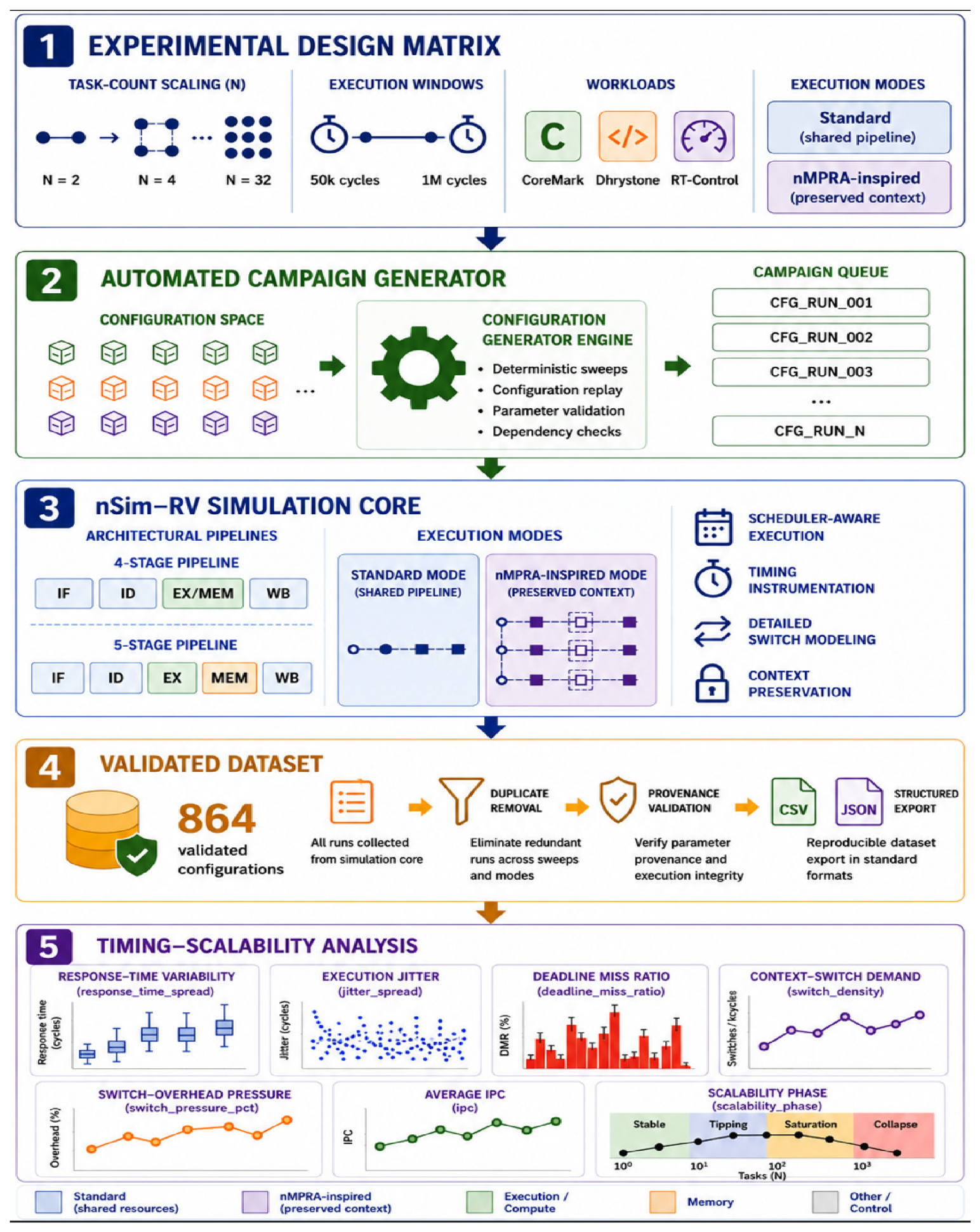
Figure 2.
Average IPC under task-count scaling for the 5-stage and 4-stage cache-disabled configurations.
Figure 2.
Average IPC under task-count scaling for the 5-stage and 4-stage cache-disabled configurations.
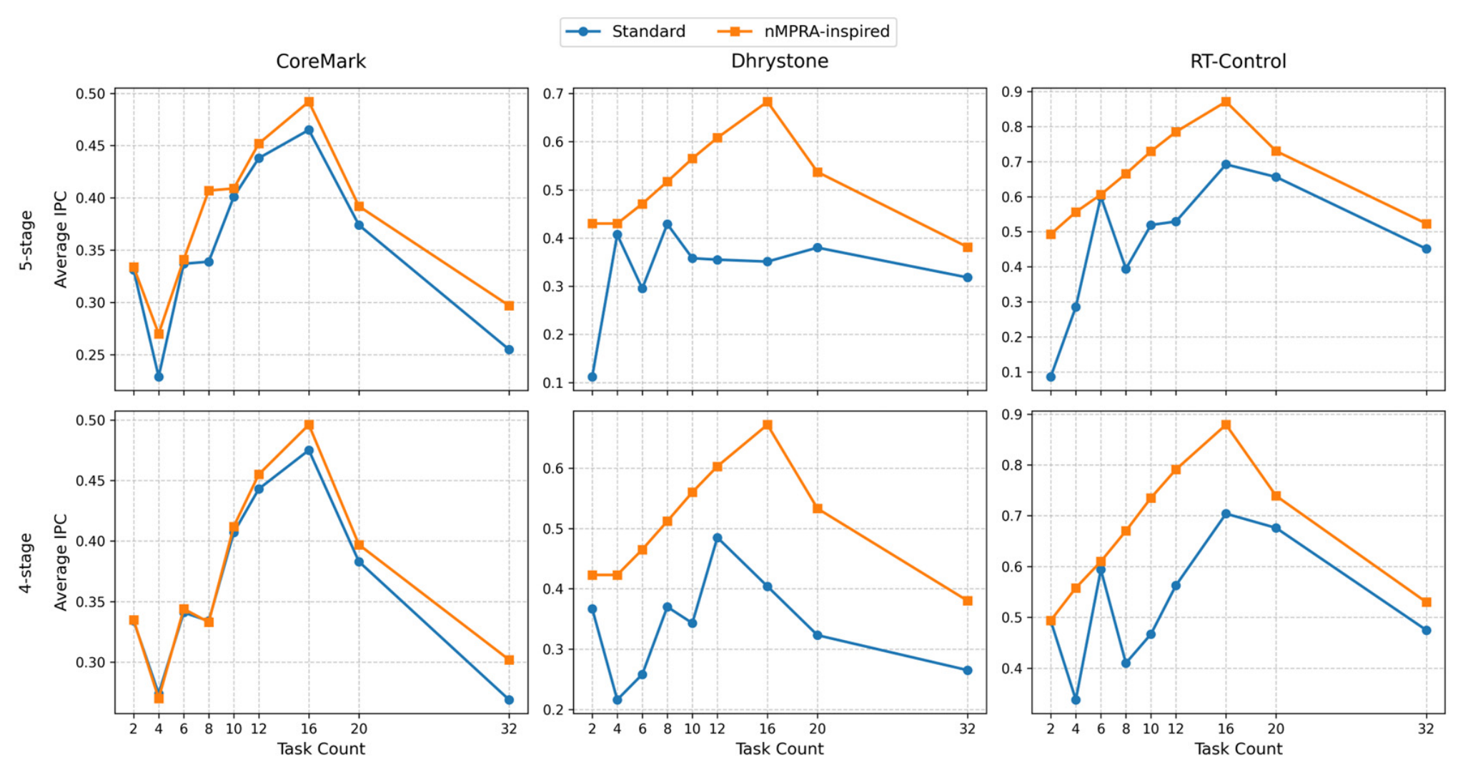
Figure 3.
Response-time variability normalized to the observation window under task-count scaling for the 5-stage and 4-stage cache-disabled configurations.
Figure 3.
Response-time variability normalized to the observation window under task-count scaling for the 5-stage and 4-stage cache-disabled configurations.
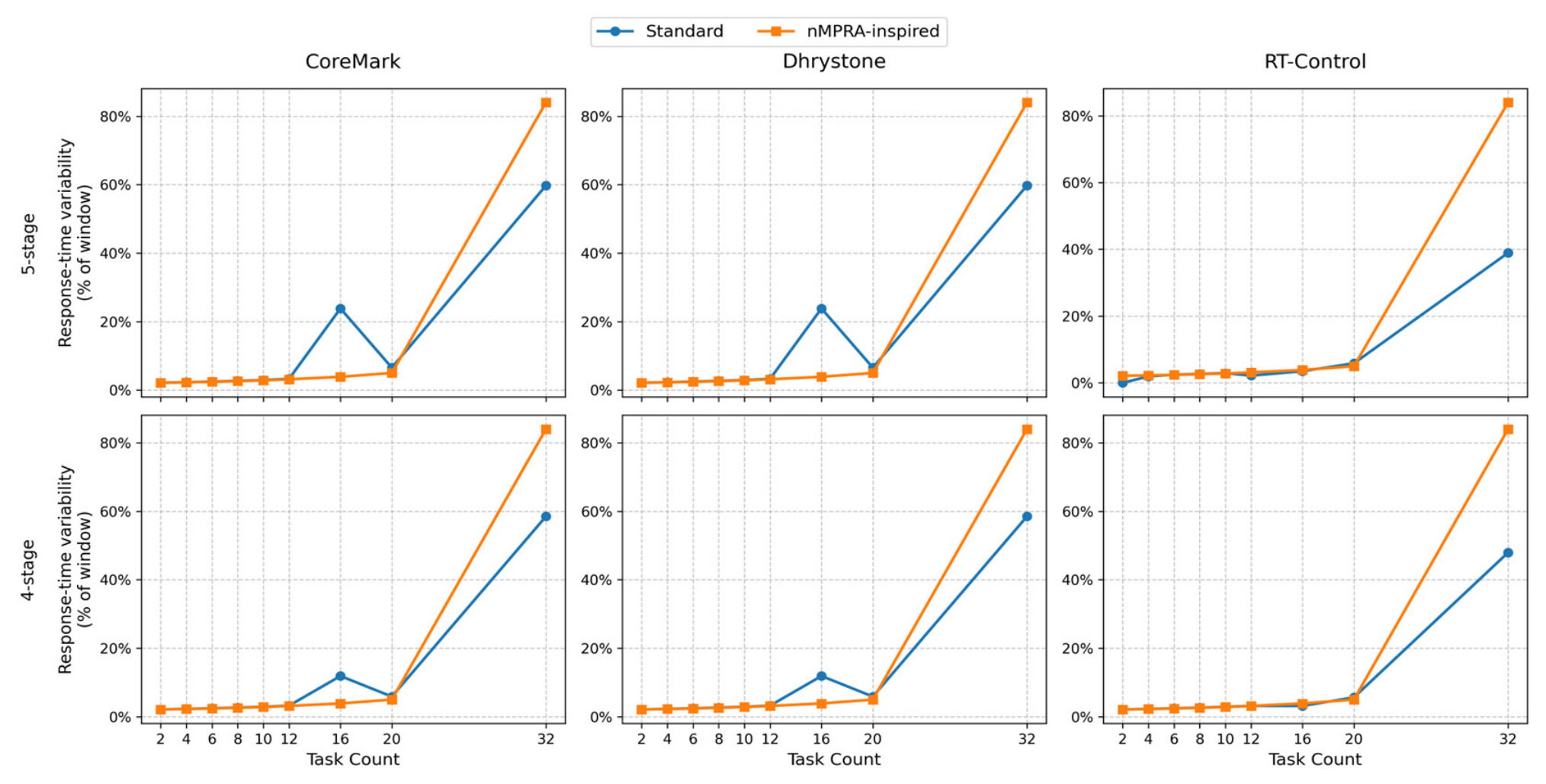
Figure 4.
Execution jitter normalized to the observation window under task-count scaling for the 5-stage and 4-stage cache-disabled configurations.
Figure 4.
Execution jitter normalized to the observation window under task-count scaling for the 5-stage and 4-stage cache-disabled configurations.
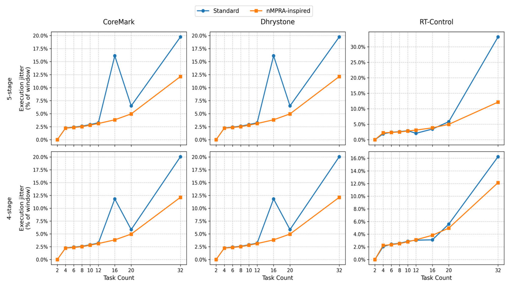
Figure 5.
Deadline miss ratio under task-count scaling for the 5-stage and 4-stage cache-disabled configurations.
Figure 5.
Deadline miss ratio under task-count scaling for the 5-stage and 4-stage cache-disabled configurations.
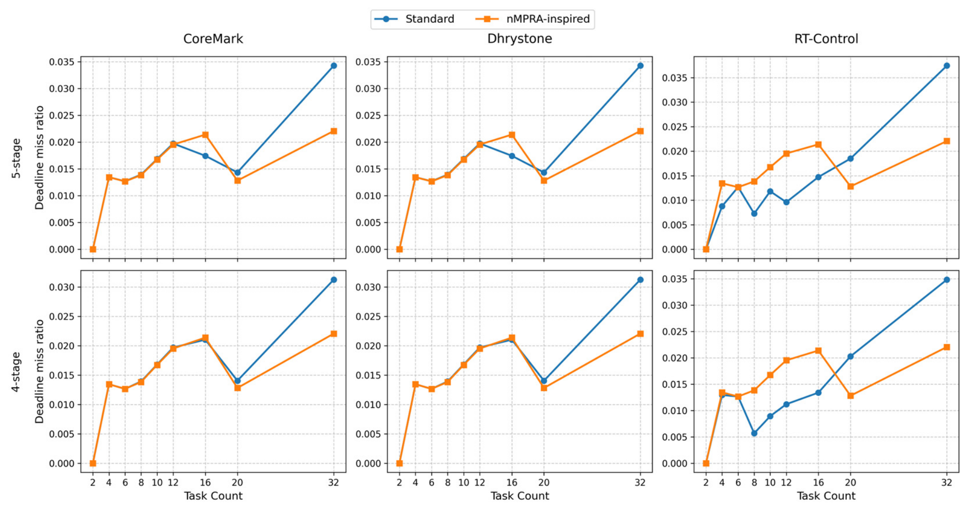
Figure 6.
Modeled switch-overhead pressure under task-count scaling for the 5-stage and 4-stage cache-disabled configurations.
Figure 6.
Modeled switch-overhead pressure under task-count scaling for the 5-stage and 4-stage cache-disabled configurations.
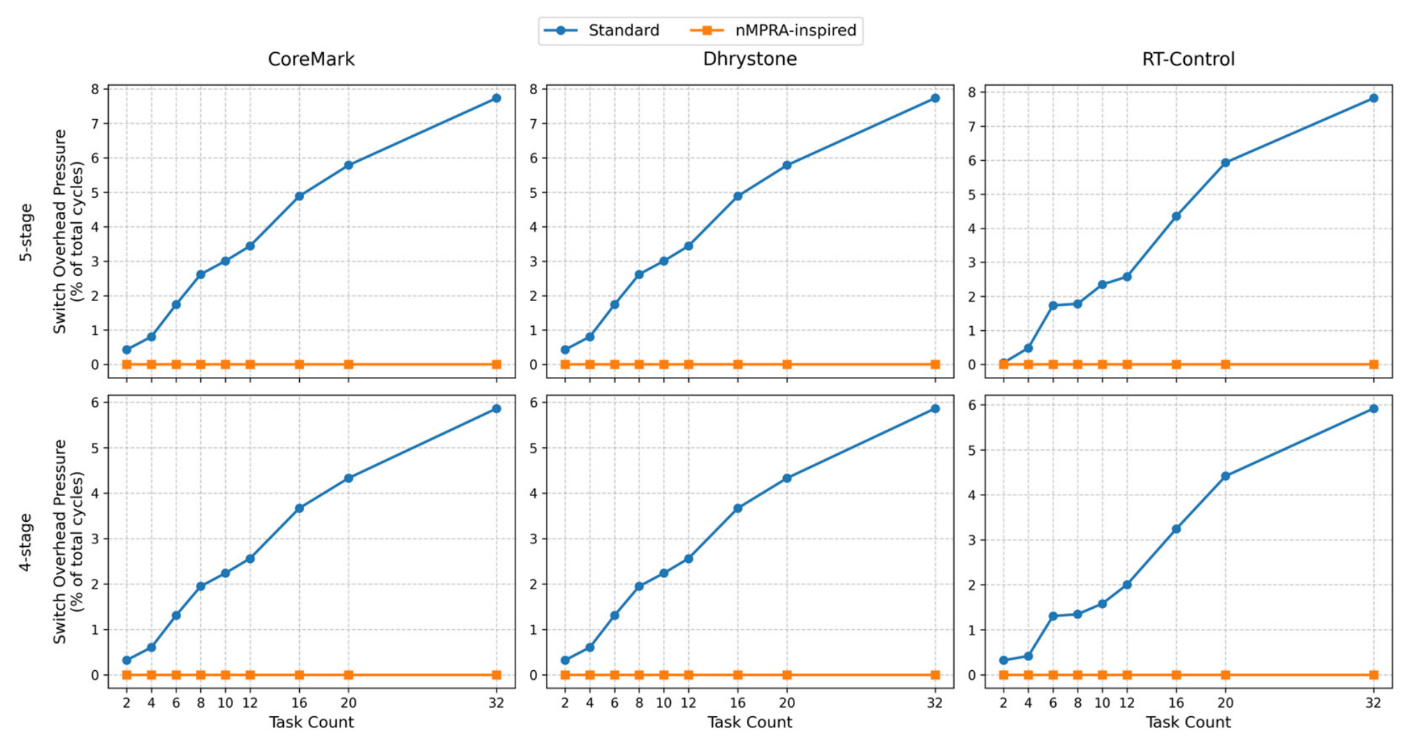
Figure 7.
Operational scalability phases under task-count scaling for the 5-stage and 4-stage cache-disabled configurations.
Figure 7.
Operational scalability phases under task-count scaling for the 5-stage and 4-stage cache-disabled configurations.
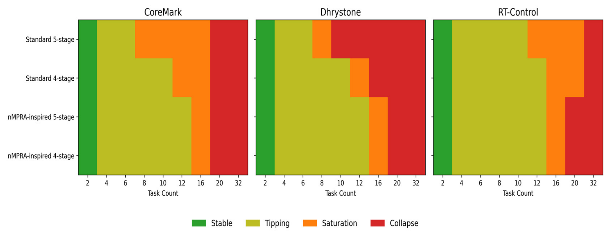
Figure 8.
Cache-induced variation in average IPC and deadline miss ratio for the 5-stage pipeline under the 1M-cycle observation window. Values are computed as Cache ON minus Cache OFF.
Figure 8.
Cache-induced variation in average IPC and deadline miss ratio for the 5-stage pipeline under the 1M-cycle observation window. Values are computed as Cache ON minus Cache OFF.
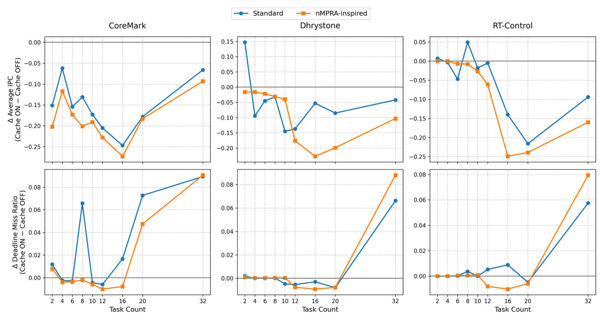

Table 1.
Positioning of nSim-RV relative to representative RISC-V simulation and evaluation environments.
Table 1.
Positioning of nSim-RV relative to representative RISC-V simulation and evaluation environments.
| Capability / Methodological Focus | gem5 [1] | FireSim [2] | GVSoC [3] | nSim-RV |
|---|---|---|---|---|
| Architectural exploration | Primary focus | Supported | Supported | Supported |
| Functional validation | Supported | Supported | Supported | Supported |
| Full-system software execution | Supported | Primary focus | Supported | Not targeted |
| FPGA-accelerated simulation | Not targeted | Primary focus | Not targeted | Not targeted |
| Fast embedded/IoT virtual platform | Limited | Limited | Primary focus | Not targeted |
| Scheduler-aware timing evaluation | Possible through customization | Possible through customization | Limited / requires extensions | Primary focus |
| Response-time variability analysis | Possible through customization | Possible through customization | Limited / requires extensions | Native workflow |
| Execution jitter analysis | Possible through customization | Possible through customization | Limited / requires extensions | Native workflow |
| Deadline-miss characterization | Possible through customization | Possible through customization | Limited / requires extensions | Native workflow |
| Context-switch and switch-overhead evaluation | Possible through customization | Possible through customization | Limited / requires extensions | Native workflow |
| Automated campaign orchestration | External workflow | External workflow | External workflow | Native workflow |
| Dataset aggregation and validation | External workflow | External workflow | External workflow | Native workflow |
| Scalability-phase characterization | Not primary focus | Not primary focus | Not primary focus | Native workflow |
Table 2.
nSim-RV experimental orchestration stages and generated artifacts.
| Stage | Role in the workflow | Main inputs | Main outputs |
|---|---|---|---|
| Experimental design | Defines the evaluation space across workload, timing, and execution parameters | Workload profiles, task-count settings, observation windows, execution modes, pipeline settings, cache settings | Configuration matrix |
| Campaign generation | Expands the design matrix into executable simulation scenarios | Configuration matrix, workload binaries, task definitions | Generated simulation configurations |
| Simulation execution | Executes each scenario under the selected nSim-RV configuration | Generated configurations, simulator executable, workload inputs | Raw logs, per-run JSON/CSV outputs |
| Result aggregation | Merges per-run outputs into structured datasets | Raw simulation outputs, scalability result files | Aggregated CSV/JSON datasets |
| Dataset validation | Removes repeated configurations and verifies metadata consistency | Merged datasets, configuration metadata | Final evaluation dataset |
| Timing analysis | Derives timing-scalability indicators from validated data | Final evaluation dataset | Response-time, jitter, deadline, context-switch, switch-overhead, and scalability-phase analyses |
Table 3.
RT-Control workload-generation paths used in the evaluation.
| Aspect | Unified scalability sweep | C1–C4 scenario path |
|---|---|---|
| Purpose | Continuous task-count scalability evaluation | Targeted validation scenarios |
| Task-count support | Supports N = 2 and the selected scalability counts generated from the template pool | Starts from four-task JSON scenarios; does not support N < 4 |
| Generation rule | Select the first N templates from a fixed task-template pool | Replicates the four-task base configuration for larger task sets |
| N = 2 generation | Generated by selecting the first two templates from the pool | Not supported |
| Example N = 2 tasks | T0: priority 1, WCET 20000, period 40000, release 0; T1: priority 2, WCET 50, period 1000, release 0 | Not applicable |
| Timing parameters | Defined by template-pool entries | Defined by explicit JSON scenario files |
| Scaling behavior | Task set grows by deterministic template selection | Periods and implicit deadlines are scaled by replication factors; execution budgets are preserved |
| Deadline model | Defined by generated task templates | Implicit deadlines equal to periods in nominal scenarios; explicit constrained deadlines in tight-deadline scenarios |
| Cross-mode consistency | Same generated task set for Standard and nMPRA-inspired modes | Same scenario definition for Standard and nMPRA-inspired modes |
Table 4.
Experimental dimensions used in the nSim-RV scalability evaluation.
| Dimension | Values used in this study | Role in the evaluation |
|---|---|---|
| Workload class | CoreMark, Dhrystone, RT-Control | Covers compute-oriented, branch/control-flow-sensitive, and synthetic control-oriented periodic behavior |
| Task-count scaling | N = 2, 4, 6, 8, 10, 12, 16, 20, 32 | Evaluates timing behavior under increasing scheduler-managed workload density |
| Observation windows | 50k, 100k, 500k, 1M cycles | Captures timing behavior over bounded and longer execution intervals |
| Execution modes | Standard, nMPRA-inspired | Compares shared-pipeline and preserved-context execution organizations |
| Pipeline organizations | 5-stage reference matrix; 4-stage parity matrix | Evaluates timing-scalability behavior under matched pipeline-depth configurations |
| Cache modes | OFF, ON | Separates the controlled scheduler-driven baseline from cache-enabled robustness evaluation |
Table 5.
Timing-oriented metrics used in the scalability evaluation.
| Metric | Dataset column | Interpretation |
|---|---|---|
| Response-time variability | response_time_spread | Spread between best-case and worst-case observed task response behavior |
| Execution jitter | jitter_spread | Activation-to-activation timing variation under scheduler-controlled execution |
| Deadline miss ratio | deadline_miss_ratio | Normalized deadline violations across task-count and observation-window configurations |
| Context-switch demand | switch_density | Scheduler-requested context-switch intensity used as a validation indicator |
| Switch-overhead pressure | switch_pressure_pct | Fraction of simulated cycles accounted for by modeled explicit switch-overhead cycles |
| Average IPC | ipc | Secondary throughput reference based on retired instructions per cycle |
| Scalability phase | scalability_phase | Operational stable, tipping, saturation, and collapse classification |
Table 6.
Operational scalability-phase classification used in this study.
| Phase | Operational criterion | Interpretation |
|---|---|---|
| Stable | No tipping, saturation, or collapse condition is met; switch-overhead pressure < 1.0% and deadline miss ratio < 0.005 | Low-pressure region with bounded scheduler-induced disturbance |
| Tipping | Switch-overhead pressure ≥ 1.0% or deadline miss ratio ≥ 0.005, provided saturation and collapse conditions are not met | Onset of measurable scheduler-induced timing stress |
| Saturation | Switch-overhead pressure ≥ 2.5% or deadline miss ratio ≥ 0.02, provided collapse condition is not met | Sustained timing stress with persistent switch-overhead or deadline pressure |
| Collapse | IPC peak ratio < 0.90 or deadline miss ratio > 0.05 | High-pressure region with strong throughput degradation relative to the trajectory peak or severe deadline pressure |
Table 7.
Aggregated scalability dataset and validation rules.
| Item | Description |
|---|---|
| Primary scalability matrix | 432 unique 5-stage configurations |
| Pipeline-depth parity matrix | 432 unique 4-stage configurations |
| Combined validated configuration set | 864 validated pipeline-specific configurations |
| Workloads | CoreMark, Dhrystone, RT-Control |
| Execution modes | Standard, nMPRA-inspired |
| Task counts | N = 2, 4, 6, 8, 10, 12, 16, 20, 32 |
| Observation windows | 50k, 100k, 500k, 1M cycles |
| Cache modes | OFF, ON |
| Output formats | CSV and JSON |
| Composite configuration key | Pipeline stage count, execution mode, workload, task count, observation window, cache mode, scenario label where applicable |
| Duplicate handling | One authoritative result retained per unique configuration |
| Validation purpose | Configuration consistency, duplicate removal, metric availability, and reproducible timing analysis |
Disclaimer/Publisher’s Note: The statements, opinions and data contained in all publications are solely those of the individual author(s) and contributor(s) and not of MDPI and/or the editor(s). MDPI and/or the editor(s) disclaim responsibility for any injury to people or property resulting from any ideas, methods, instructions or products referred to in the content. |
© 2026 by the authors. Licensee MDPI, Basel, Switzerland. This article is an open access article distributed under the terms and conditions of the Creative Commons Attribution (CC BY) license.
Copyright: This open access article is published under a Creative Commons CC BY 4.0 license, which permit the free download, distribution, and reuse, provided that the author and preprint are cited in any reuse.