

Submitted:
03 June 2026
Posted:
04 June 2026
You are already at the latest version
Abstract
In an era where compute resources are rapidly advancing with better algorithms and larger clusters, the growth of labeled data, the fossil fuel of AI, has not kept pace. This disparity has spurred a growing interest in learning paradigms that rely solely on unlabeled data. A class of these paradigms employ unsupervised learning objectives that operate directly in the probability or prediction space, with Shannon entropy being one common example among many. Such objectives leverage unlabeled domain data to enable diverse tasks within the target domain. Yet, these methods remain scattered across the literature, with no systematic overview to guide their comparison or use. This work addresses that gap by providing a high-level compilation of the designs, implementations, and applications of 17 such unsupervised loss functions, focusing on their roles in common learning applications while also exploring their broader potential. By presenting their theoretical underpinnings, practical applications, and small-scale yet extensive experiments, this study aims to shape future research by addressing data scarcity, reducing dependence on labeled annotations, and enabling the unsupervised optimization of increasingly large models.
Keywords:
information theory
; unsupervised objectives
; machine learning
; classification
1. Introduction

The growth of compute, model scale, and optimization infrastructure has outpaced the growth of labeled data. In many application domains, annotation remains the dominant bottleneck rather than computation. When target-domain labels are scarce [1], a common strategy is to transfer models pre-trained on abundant labeled source-domain data [2]. The limitation is well known: domain shift between source and target distributions can substantially reduce performance on out-of-distribution (OOD) inputs [3]. A disease diagnostic system trained on one distribution, for example, may fail when the target population or acquisition process changes [4]. These constraints have renewed interest in unsupervised and zero-shot adaptation methods that update a model, or an attached module, without target labels [5,6,7]. Many such methods operate without source data and sometimes without additional supervised training, instead optimizing objectives defined directly in the probability space [8].
Figure 1.
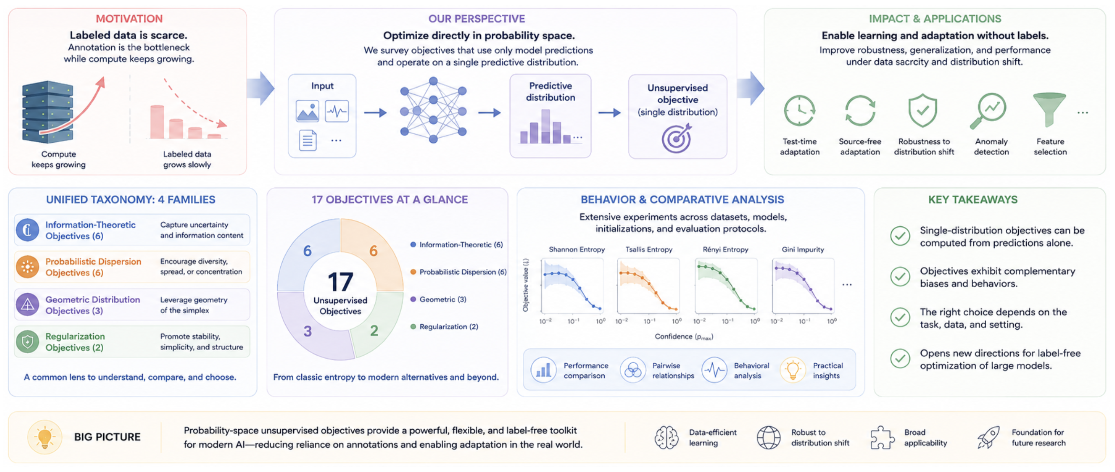
Overview of probability-space unsupervised objectives for label-free learning. The survey organizes 17 objectives into four families: information-theoretic, probabilistic dispersion, geometric, and regularization-based, and analyzes their behavior, relationships, and practical applications using a unified predictive-distribution perspective. By enabling optimization directly from model predictions, these objectives offer a versatile framework for adaptation, robustness, and learning in data-scarce environments.
Figure 1.
Overview of probability-space unsupervised objectives for label-free learning. The survey organizes 17 objectives into four families: information-theoretic, probabilistic dispersion, geometric, and regularization-based, and analyzes their behavior, relationships, and practical applications using a unified predictive-distribution perspective. By enabling optimization directly from model predictions, these objectives offer a versatile framework for adaptation, robustness, and learning in data-scarce environments.
1.1. Motivation
A broad class of unsupervised objectives acts on a single predictive distribution rather than on paired labels, paired samples, or paired domains. Shannon entropy is the most familiar example, but it is only one member of a larger design space spanning information-theoretic, dispersion-based, geometric, and regularization-based formulations. These objectives have appeared in applications ranging from feature selection and anomaly detection to test-time adaptation and source-free adaptation. Their role in modern AI systems, including large language models such as GPT [9] and BERT [10], and vision-language models such as CLIP [11] and Flamingo [12], is increasing but remains scattered across subfields [13]. In data-scarce settings, objectives such as Shannon and Tsallis entropy can improve robustness, reduce overfitting, and respond to domain shift [8,14,15]. More broadly, single-distribution objectives are a natural fit for unlabeled optimization because they can be computed directly from model predictions [16,17].
In this review, a single probability distribution refers to the conditional predictive distribution associated with one input, typically written as . The survey focuses on objectives whose primary argument is this single predictive distribution. We therefore exclude pairwise distribution losses, contrastive objectives, and divergences between two distributions except when they are needed to clarify relations among the surveyed objectives.
1.2. Objective & Impact
This survey reviews 17 foundational unsupervised objectives defined on single probability distributions. Our goal is not simply to catalogue formulas, but to clarify what each objective measures, which assumptions it makes, how it relates to nearby objectives, and where it has been used in practice. In contrast to prior reviews centered on tasks or application domains, we focus on the objective itself as the unit of analysis, with emphasis on theory, implementation, and practical selection [8].
The impact of this scope extends beyond classical unsupervised learning. In large language models, such objectives can support adaptation and fine-tuning under limited supervision, including settings involving low-resource languages [10]. In vision-language systems, they can regularize confidence, encourage diversity, or help align representations in unlabeled target domains. More generally, probability-space objectives expose compact levers for controlling uncertainty, concentration, diversity, and structure, which makes them relevant to robustness, fairness, efficiency, and interpretability in modern AI systems.
1.3. Contribution and Outline
This review consolidates probability-space unsupervised objectives into a single framework and evaluates them from both a theoretical and a practical perspective. Compared with the original draft, the revised version is more synthesis-oriented: it reduces repetition, highlights algebraic relations across objectives, and makes explicit which objectives are truly distinct and which are reparameterizations or reinterpretations of the same primitive.
Our contributions are as follows:
- Taxonomy and synthesis. We organize 17 objectives into four families and describe the design principles that distinguish them.
- Theoretical clarification. We make explicit the relations among closely related objectives, including normalized, exponential, quadratic, and moment-based variants.
- Practical guidance. We summarize computational properties, implementation considerations, and task-level suitability, and we preserve direct pointers to implementation through the existing project assets.
- Empirical comparison. We retain the small-scale controlled experiments to illustrate how different unsupervised objectives behave when used directly for unlabeled optimization.
- Forward-looking discussion. We connect the surveyed objectives to current adaptation settings in large pre-trained models and identify promising directions for future work.
The remainder of the paper follows the same backbone as the original manuscript with minor structural tightening. Section 2 defines the scope, introduces the single-probability setting, and positions this survey relative to prior reviews. Section 3 presents the objective families. Section 4 reports the comparative experiments. Section 5 synthesizes practical lessons, comparative behavior, and future directions. Section 6 and Section 7 conclude the paper and discuss validity threats.
2. Background
2.1. Evolution of Learning Objectives
The history of learning objectives mirrors the history of machine learning itself. Early work, especially in statistics and information theory, introduced measures of uncertainty, surprise, spread, and concentration. As machine learning moved toward more complex predictive tasks, these measures became useful not only for analysis but also for optimization. Entropy-based objectives formalized uncertainty. Dispersion measures quantified variability. Moment-based quantities such as skewness and kurtosis described shape. Regularization terms provided a way to control model complexity and prevent brittle overconfident predictions.
The deep learning era amplified all of these needs. High-capacity models required stronger regularization, better confidence control, and principled ways to adapt under domain shift. At the same time, the cost of annotation motivated unsupervised and self-supervised methods. The recent rise of source-free adaptation, test-time adaptation, and adaptation of large pre-trained models has therefore brought single-distribution objectives back to the foreground. Figure 2 summarizes this evolution and shows that many “new” objectives are modern uses of older statistical principles rather than entirely new inventions.
2.2. Single Probability Distribution (SPD)
The common object underlying this survey is the conditional predictive distribution , which assigns a probability to each possible outcome for a given input. This perspective is especially natural in zero-shot, transfer, and adaptation settings because the model already produces probabilities even when labels are unavailable.
Definition 1.
Let be a sample from a distribution X, and let denote the corresponding label. The conditional probability distribution is given by Bayes’ rule:
Here, is the likelihood, is the prior, and is the marginal likelihood. In discriminative models, the same object is usually parameterized directly. For multiclass prediction,
where is the logit for class and are model parameters. Prediction is typically obtained by
This formulation provides the substrate on which the surveyed objectives operate. Some objectives treat the predictive distribution as a categorical object and are invariant to class permutations; others require an ordered or numeric support and therefore depend on how outcomes are encoded.
2.3. Related Works
Several prior surveys review loss functions or unsupervised learning more broadly. [18] surveys loss functions across supervised, unsupervised, and reinforcement learning. [19] focuses on clustering and dimensionality reduction. [20] provides a broad review of loss functions across domains. [21] studies unsupervised losses for homography estimation in geometric computer vision. [22] surveys unsupervised methods in supply-chain settings. These works are useful but they do not focus specifically on objectives whose input is a single probability distribution.
That omission matters. Objectives such as Shannon entropy [23] provide direct control over uncertainty, diversity, or concentration in predictive outputs, and they are now central to modern adaptation settings including large pre-trained models [11,13,14]. The present survey therefore complements prior reviews by taking the predictive distribution itself as the organizing principle.

Table 1.
Comparison of related review works on unsupervised loss (UL) functions and their focus. Single Distribution indicates whether the UL function inputs a single probability distribution, making it more applicable in state-of-the-art settings, while Comments indicates a positive or negative aspect of each review work.
Table 1.
Comparison of related review works on unsupervised loss (UL) functions and their focus. Single Distribution indicates whether the UL function inputs a single probability distribution, making it more applicable in state-of-the-art settings, while Comments indicates a positive or negative aspect of each review work.
| Ref | Year | UL | Single Distribution | Focus of Review | Comments |
|---|---|---|---|---|---|
| [18] | 2023 | ✓ | ✗ | Broad survey of loss functions across tasks | Task-specific taxonomy |
| [19] | 2022 | ✓ | ✗ | Clustering and dimensionality reduction | Descriptive without analysis |
| [20] | 2020 | ✓ | ✗ | Theoretical analysis and taxonomy | Naively discussed 4 UL functions |
| [21] | 2021 | ✓ | ✗ | Applications in geometric computer vision | Briefly analyzed just 2 UL functions |
| [22] | 2024 | ✓ | ✗ | Optimization in supply chain systems | A certain use-case focused |
| Ours | 2024 | ✓ | ✓ | Single Probability Distribution Losses | Demonstrated extensive experiments |
2.4. Taxonomy of Objectives
We organize the surveyed objectives into four families: Information Theory-based losses, Probabilistic Dispersion-based losses, Geometric Distribution-based losses, and Regularization-based losses. The taxonomy reflects both mathematical form and functional role.
Information-theoretic objectives measure uncertainty, surprise, or coding length. Probabilistic-dispersion objectives quantify spread, impurity, dominance, or complexity. Geometric objectives capture higher-order distributional shape and therefore require an ordered support. Regularization objectives are best interpreted as inductive biases: they do not simply measure a property of the predictive distribution, but actively prefer smoother, more concentrated, or sparser outputs. Figure 3 provides the resulting hierarchy.
3. Unsupervised Objectives for SPDs
3.0 Preliminary
3.0.1. Assumption
Unless stated otherwise, we assume a discrete predictive distribution
When an objective requires numeric support, we write the associated support values as . This distinction matters because some objectives are permutation-invariant over class labels, while others are not.
3.0.2. Exemplary Illustration
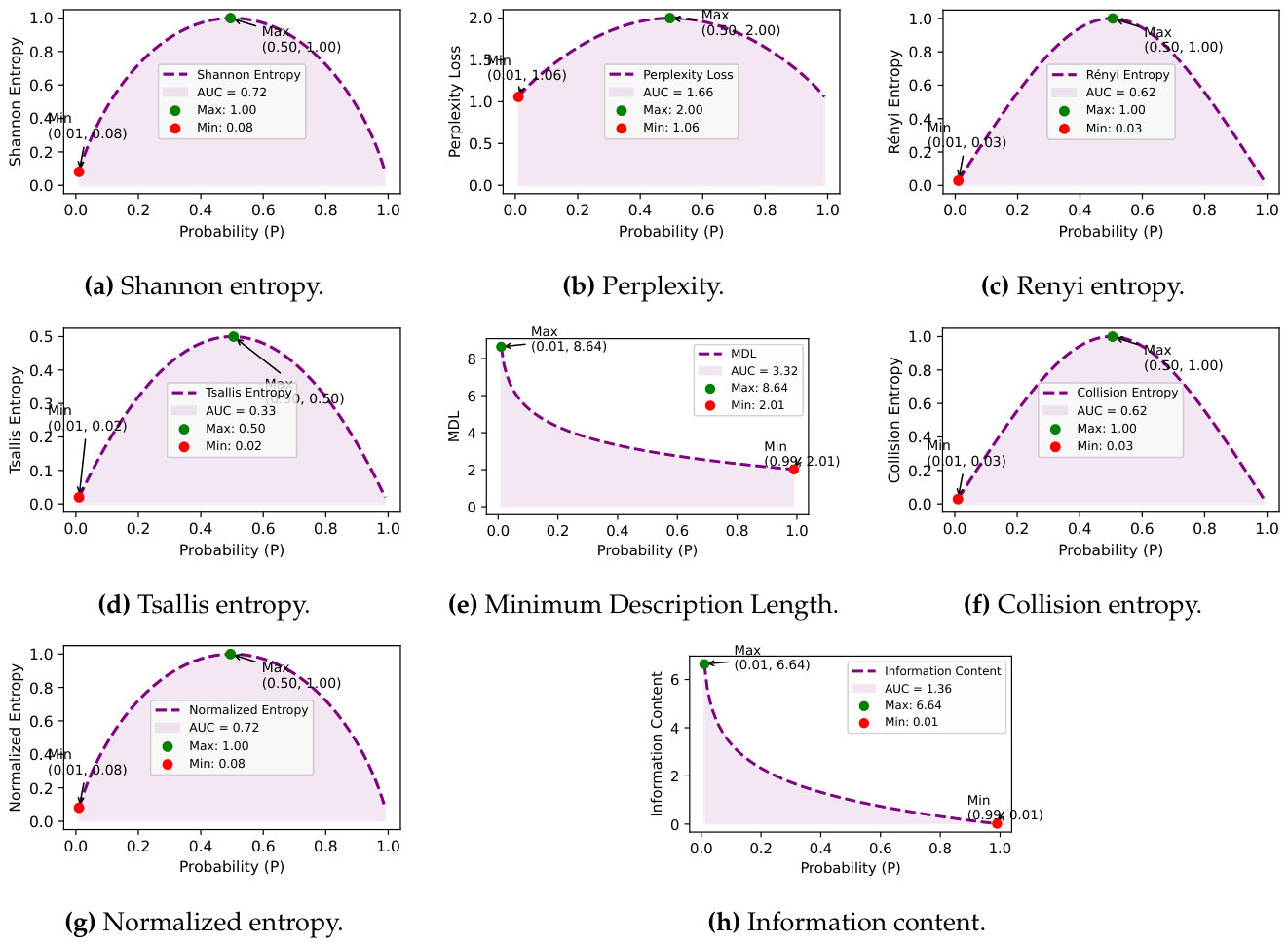
The curve plots used throughout this survey evaluate each objective on a simple one-dimensional probability sweep. Concretely, we consider probabilities and visualize how each objective varies with concentration, uncertainty, or shape. These plots are not substitutes for full optimization analysis, but they provide an interpretable first view of monotonicity, symmetry, and extreme-value behavior.
3.0.3. Notations
Unless stated otherwise, logarithms are natural, in which case values are expressed in nats; base-2 logarithms yield bits [24]. We use the term objective rather than loss when the sign convention depends on implementation, since several quantities in this survey are maximized in analysis but minimized in optimization by negating them.
3.1. Information Theory Losses
Information-theoretic objectives are the most widely used probability-space objectives in modern adaptation pipelines. They directly quantify uncertainty, coding length, or surprise. Many are closely related: perplexity is the exponential form of Shannon entropy; collision entropy is a special case of Renyi entropy; normalized entropy rescales Shannon entropy; and information content is the pointwise term whose expectation gives Shannon entropy.
3.1.1. Shannon Entropy
Shannon entropy measures the uncertainty of a predictive distribution [23,25]. For a discrete SPD,
with maximum value under the uniform distribution and minimum value at a point mass. The computation is linear in the number of outcomes, , and the quantity is invariant to permutations of the class labels [26].
In machine learning, Shannon entropy underlies information-gain criteria for tree induction [27], clustering criteria [28], and entropy-minimization schemes for adaptation [6,29]. It also appears in language modeling and generation [30,31], anomaly detection [32], domain generalization [33], and zero-shot or test-time adaptation of vision-language models [13,14]. Its appeal comes from the fact that it is simple, stable, and often acts as a reliable confidence-control signal.
3.1.2. Perplexity Loss
Perplexity measures the effective number of equally likely outcomes and is the exponential form of base-2 Shannon entropy [23,34]:
Lower perplexity corresponds to more concentrated and predictable predictions. Because it is computed from entropy, its complexity is also .
Perplexity is standard in generative modeling and natural language processing. It is widely used to evaluate and guide recurrent language models [35], large generative models [31,36], and transformer-based pre-trained models such as BERT [10]. Relative to raw entropy, its main advantage is interpretability: the value can be read as an effective support size.
3.1.3. Rényi Entropy
Rényi entropy generalizes Shannon entropy by introducing an order parameter that controls how strongly the objective emphasizes large or small probabilities [25]:
As , it converges to Shannon entropy. Larger values emphasize dominant probabilities; smaller values emphasize the tail. The cost remains , with minor overhead from exponentiation.
This tunability makes Rényi entropy useful in settings where one wants to control sensitivity to concentration or rarity. Representative uses include regularization in neural networks [37,38], quantum information and entanglement analysis [39,40], adaptive learning in dynamic neural systems [41,42], and variational estimation of distributions and divergences [43].
3.1.4. Tsallis Entropy
Tsallis entropy is another one-parameter generalization of Shannon entropy, designed for non-extensive settings in which classical additivity is not the preferred assumption [44,45]:
It converges to Shannon entropy as . Like Rényi entropy, it remains an objective, but its parameterization often yields a different practical sensitivity to concentration and outliers.
Tsallis entropy has been used in imbalanced decision trees and robust learning [46], anomaly detection [47], ecological diversity analysis [48], text-domain adaptation [49], and quantum-information settings [50]. In practice, it is attractive when the target domain exhibits heavy tails, imbalance, or atypical concentration patterns.
3.1.5. Minimum Description Length (MDL)
The Minimum Description Length principle occupies a boundary between information-theoretic objective and model-selection criterion. Its core idea is to minimize total code length by trading data fit against model complexity [51,52,53]:
Unlike the other information-theoretic objectives in this section, MDL is not determined solely by the predictive distribution; it also depends on how model complexity is encoded. This distinction is important when comparing MDL to purely distributional quantities.
MDL appears in few-shot and transductive inference [54], reinforcement learning [55], spiking neural networks [56], dimension reduction [57], prompt and parameter-efficient tuning [58], and analyses of intrinsic dimensionality in language-model fine-tuning [59]. Its main strength is principled control of overfitting through compression.
3.1.6. Collision Entropy
Collision entropy is the order-2 case of Rényi entropy and measures concentration through pairwise collisions [60,61,62]:
The quadratic term makes the objective especially sensitive to dominant probabilities. Computation is , and the objective is permutation-invariant over categories.
Collision entropy is widely used in cryptography and security analysis [60,63,64]. It also appears in ecological dominance analysis [65] and as a sharpness-sensitive diagnostic in machine learning [66]. Relative to Shannon entropy, it emphasizes overlap and concentration rather than average uncertainty.
3.1.7. Normalized Entropy
Normalized entropy rescales Shannon entropy to the interval , making comparisons across different support sizes more direct [23,67]:
This simple normalization preserves the ordering induced by Shannon entropy while eliminating dependence on the number of categories. The computational cost is again .
Normalized entropy is useful when support size varies across tasks or datasets. Representative applications include clustering evaluation [68], biodiversity analysis [69], and feature ranking based on relative uncertainty reduction [70]. In survey terms, it is best viewed as a reporting and comparison layer over Shannon entropy rather than a fundamentally different primitive.
3.1.8. Information Content
Information content is the pointwise surprise associated with a single event [23,67,71]:
Its expectation under P recovers Shannon entropy. For a single event the computation is ; evaluating it over all outcomes is .
Because it is event-specific rather than distribution-averaged, information content can be useful when rare outcomes must be emphasized. It is central to coding theory [72], appears in language and text modeling [68], and can be used in decision-making or reinforcement learning to value informative outcomes [73,74]. The experiments in this paper also show that this emphasis on rare events can be destabilizing when used naively as an adaptation objective.
Table 2.
Summary of information theory-based unsupervised objectives that take a single probability distribution with n outcomes as input. Min and Max represent the minimum and maximum possible values for n outcomes, AUC represents the possible area under the curve of the objective’s value across distributions, and Monotonicity describes the behavior of the objective as probabilities approach 1, where represents the probability assigned to the i-th outcome of a discrete probability distribution P.
Table 2.
Summary of information theory-based unsupervised objectives that take a single probability distribution with n outcomes as input. Min and Max represent the minimum and maximum possible values for n outcomes, AUC represents the possible area under the curve of the objective’s value across distributions, and Monotonicity describes the behavior of the objective as probabilities approach 1, where represents the probability assigned to the i-th outcome of a discrete probability distribution P.
| Unsupervised Objective | Min | Max | AUC | Monotonicity | Key Characteristics |
|---|---|---|---|---|---|
| Shannon Entropy [Eq. 4] | 0 | Finite | Decreasing for | Measures uncertainty in distributions. | |
| Perplexity Loss [Eq. 5] | 1 | n | Finite | Decreasing for | Measures effective number of outcomes. |
| Rényi Entropy () [Eq. 6] | 0 | Finite | Varies with | Generalizes Shannon Entropy. | |
| Tsallis Entropy () [Eq. 7] | 0 | Finite | Varies with q | Generalizes Shannon Entropy with q. | |
| Minimum Description Length [Eq. 8] | Unbounded | N/A | Varies | Measures complexity of data encoding. | |
| Collision Entropy [Eq. 9] | 0 | Finite | Decreasing for | Based on pairwise collisions in P. | |
| Normalized Entropy [Eq. 10] | 0 | 1 | Finite | Decreasing for | Normalized measure of uncertainty. |
| Information Content [Eq. 11] | 0 | ∞ | Infinite | Decreasing for | Negative log-probability of events. |
Figure 4.
Objective curves for the information-theoretic family.
3.2. Probabilistic Dispersion Losses
Probabilistic-dispersion objectives quantify spread, impurity, dominance, or structural complexity. Here the support matters. Gini impurity and Simpson’s index depend only on the probabilities and are permutation-invariant. Variance and mean absolute deviation require numeric support values, so their meaning changes if categories are relabeled. Statistical complexity combines entropy with a second structural term and sits between pure dispersion and structural analysis.
3.2.1. Variance Loss
3.2.2. Gini Impurity
Gini impurity measures the probability of misclassification if labels were sampled from the predictive distribution itself [27,83,84]:
The computation is . Algebraically, Gini impurity is the complement of both Simpson’s diversity index and the quadratic regularizer discussed later, which is why these objectives often behave similarly in practice.
Its classical use is in decision trees and related splitting criteria, where lower impurity corresponds to cleaner partitions. In probability-space optimization more broadly, Gini acts as a diversity-promoting alternative to entropy with a simpler quadratic form.
3.2.3. Mean Absolute Deviation (MAD)
3.2.4. Statistical Complexity Loss
Statistical complexity attempts to capture not only uncertainty but also structural organization. A common form multiplies Shannon entropy by Fisher information [91,92,93,94]:
The exact Fisher-information term depends on parameterization, so implementations vary, but the computational burden is typically linear in the number of support points once the parameterization is fixed.
This objective has been used in time-series analysis [95], neural information-bottleneck studies [96], feature selection and compression [97], and ecological-network analysis [98]. It is best suited to settings where one wants to reward informative but nontrivial structure rather than mere uncertainty.
3.2.5. Simpson’s Diversity Index
Simpson’s Diversity Index (SDI) measures dominance by summing squared probabilities [99]:
A reciprocal form, , is also common. The raw index is identical to the L2 distribution regularizer discussed in Section 3; only the interpretation changes. In ecology and retrieval, high means dominance and low diversity, while in regularization the same quantity measures concentration.
SDI appears in diversified retrieval [100], microbiome clustering and diversity analysis [101], and ecological modeling [102,103]. Its usefulness in machine learning comes from the fact that the quadratic form is cheap, differentiable, and easy to interpret as concentration.
Figure 5.
Objective curves for the probabilistic-dispersion family.
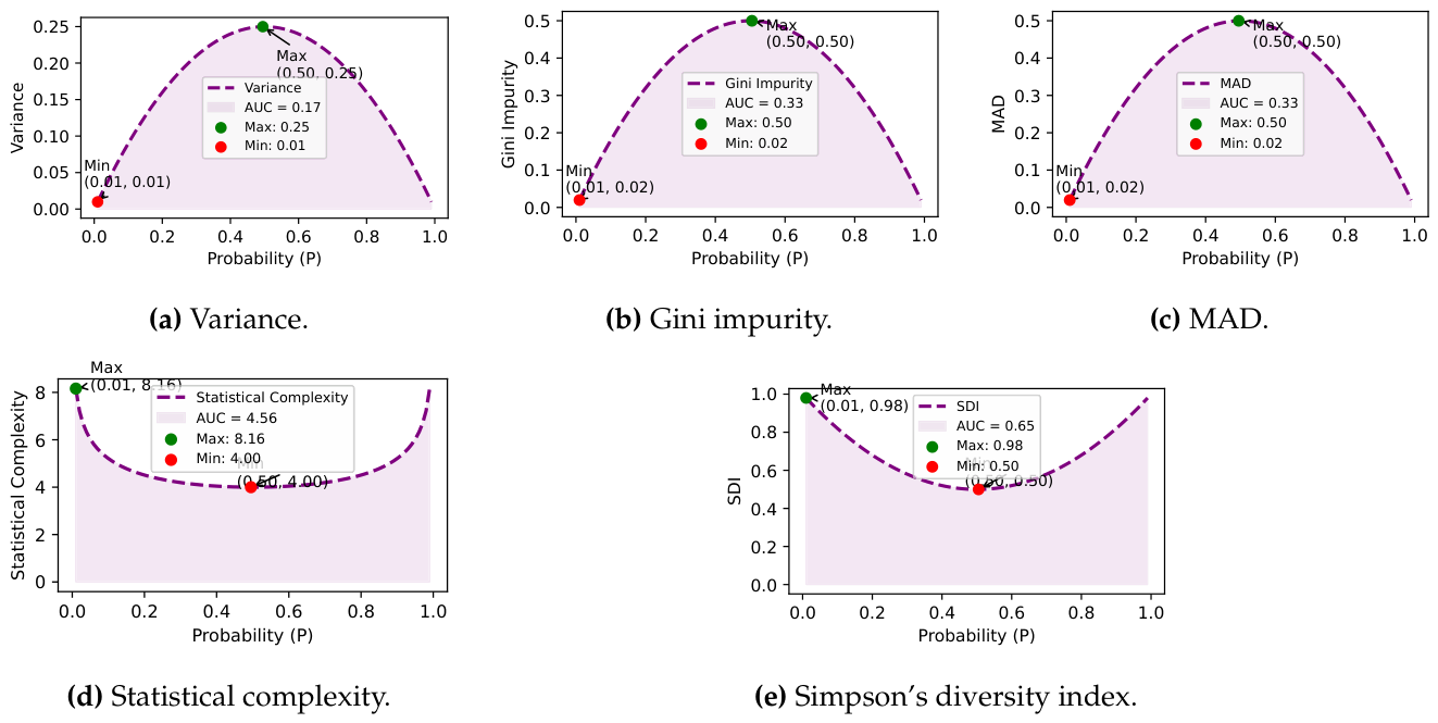
Table 3.
Summary of probabilistic dispersion-based unsupervised objectives that take a single probability distribution with n outcomes as input. Min and Max represent the minimum and maximum possible values for n outcomes, AUC represents the possible area under the curve of the objective’s value across distributions, and Monotonicity describes the behavior of the objective as probabilities approach 1, where represents the probability assigned to the i-th outcome of a discrete probability distribution P.
Table 3.
Summary of probabilistic dispersion-based unsupervised objectives that take a single probability distribution with n outcomes as input. Min and Max represent the minimum and maximum possible values for n outcomes, AUC represents the possible area under the curve of the objective’s value across distributions, and Monotonicity describes the behavior of the objective as probabilities approach 1, where represents the probability assigned to the i-th outcome of a discrete probability distribution P.
| Unsupervised Objective | Min | Max | AUC | Monotonicity | Key Characteristics |
|---|---|---|---|---|---|
| Variance Loss [Eq. 12] | 0 | Finite | Decreasing for | Measures dispersion from the mean. | |
| Gini Impurity [Eq. 13 ] | 0 | Finite | Decreasing for | Measures probability of misclassification. | |
| Mean Absolute Deviation [Eq. 14] | 0 | Finite | Decreasing for | Measures average absolute deviation from mean. | |
| Statistical Complexity Loss [Eq. 15] | Unbounded | N/A | Varies with distribution | Measures structure and unpredictability. | |
| Simpson’s Diversity Index [Eq. 16] | 1 | Finite | Decreasing for | Measures lack of diversity in distributions. |
3.3. Geometric Distribution Losses
Geometric-distribution objectives rely on higher-order moments. Unlike entropy or Gini-type quantities, they are not permutation-invariant and are meaningful only when outcomes lie on an ordered or numeric support. For categorical labels without order, they are generally not appropriate.
3.3.1. Skewness Loss
Skewness measures asymmetry around the mean [104,105]:
It is positive for right-tailed distributions and negative for left-tailed distributions. Computing it requires the mean, standard deviation, and third centered moment, which is again .
Skewness-aware objectives have been used to regularize neural activations [106], detect anomalous asymmetry [107], analyze financial-return asymmetry [108], and adapt learning under imbalance [109]. The key practical caveat is that skewness is support-dependent; it should not be interpreted on arbitrarily indexed classes.
3.3.2. Kurtosis Loss
Kurtosis measures tail heaviness or outlier sensitivity relative to a reference shape [110,111]:
The fourth power amplifies extreme deviations, which makes kurtosis highly sensitive to outliers. The cost is , but numerical stability may require care when the predictive distribution becomes extremely concentrated.
Applications include anomaly detection in multivariate time series [112], financial risk analysis [113], signal denoising [114], and robust adaptive neural models [115]. As with skewness, the quantity is meaningful only when the support has geometry.
Figure 6.
Objective curves for the geometric family.
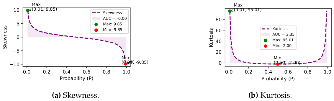
Table 4.
Summary of geometric distribution-based and regularization-based unsupervised objectives that take a single probability distribution with n outcomes as input. Min and Max represent the minimum and maximum possible values for n outcomes, AUC represents the possible area under the curve of the objective’s value across distributions, and Monotonicity describes the behavior of the objective as probabilities approach 1, where represents the probability assigned to the i-th outcome of a discrete probability distribution P.
Table 4.
Summary of geometric distribution-based and regularization-based unsupervised objectives that take a single probability distribution with n outcomes as input. Min and Max represent the minimum and maximum possible values for n outcomes, AUC represents the possible area under the curve of the objective’s value across distributions, and Monotonicity describes the behavior of the objective as probabilities approach 1, where represents the probability assigned to the i-th outcome of a discrete probability distribution P.
| Unsupervised Objective | Min | Max | AUC | Monotonicity | Key Characteristics |
|---|---|---|---|---|---|
| Skewness Loss [Eq. 17] | Undefined | Depends on distribution | Measures asymmetry of probability distributions. | ||
| Kurtosis Loss [Eq. 18] | Undefined | Varies with tail weight | Measures “peakedness” and tail behavior. | ||
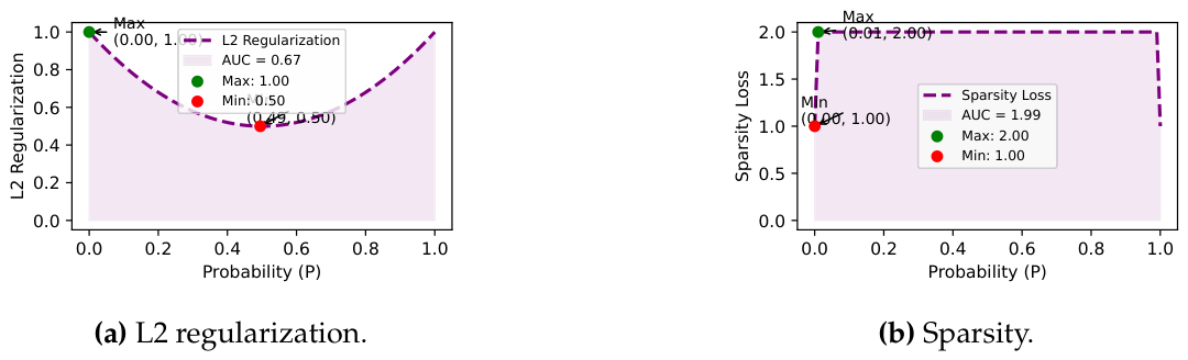
| L2 Regularization Eq. 19 | 0 | 1 | Finite | Decreasing for | Penalizes sharp distributions. |
| Sparsity Loss [Eq. 20] | 0 | n | Finite | Increasing with non-zeros | Counts non-sparse dimensions (above a threshold). |
3.4. Regularization Losses
Regularization objectives are best understood as preferences over predictive distributions. Rather than estimating uncertainty or shape for its own sake, they bias optimization toward smoother or sparser outputs. This family overlaps algebraically with other families, which is why interpretation matters.
3.4.1. L2 Distribution Regularization
L2 distribution regularization penalizes concentrated predictive distributions [116,117]:
This is the same quadratic form as Simpson’s diversity index, but here it is interpreted as an anti-overconfidence regularizer. The objective is cheap to compute, , and easy to differentiate.
Representative uses include knowledge distillation and smoothing [118], label smoothing in deep networks [117], and regularization of sequence models to reduce peaked output distributions [119]. In adaptation settings, it often serves as a practical alternative when entropy is numerically inconvenient or when one wants a purely quadratic penalty.
3.4.2. Sparsity Loss
Sparsity objectives encourage predictive distributions with only a few active entries. In idealized form,
where counts nonzero entries. The formal complexity is , but the more important issue is conceptual: for dense softmax outputs, exact zeros rarely occur, so raw sparsity is often ill-posed unless one uses thresholds, relaxed surrogates, sparse alternatives to softmax, or discrete latent variables.
Even with that caveat, sparsity remains influential in feature selection and representation learning [120,121,122]. Recent uses include sparse autoencoders for model interpretability [123], unsupervised learning with sparse priors [124], and sparse latent-variable models [125]. In adaptation problems, the main question is not whether sparsity is useful, but which relaxed formulation best matches dense predictive outputs.
Figure 7.
Objective curves for the regularization family.
4. Experiments and Analysis
4.1. Experimentation
The experiments are retained as a controlled, small-scale comparison of how the surveyed objectives behave when used directly for unlabeled optimization. The goal is illustrative rather than benchmark-driven: we use the same backbone, the same adaptation recipe, and multiple datasets to expose broad patterns rather than to claim state-of-the-art results.
4.1.1. Problem Formulation
Following [13,14], we study image classification under unlabeled optimization. Given an image x, a model produces predictive probabilities . Instead of using ground-truth labels, we compute an unsupervised objective directly from the predictive distribution and update the parameters through
The comparison is therefore between the original model and the model after objective-driven optimization, . This setup mirrors common test-time and source-free adaptation recipes [13,14,29] while remaining simple enough for controlled comparison.
4.1.2. Experimental Setup
We evaluate on CIFAR-10, MNIST, Fashion-MNIST, and SVHN, each with 10 classes. For tractability, 2,000 samples are drawn from each dataset and split 80:20 for training and testing. Two initialization settings are used. In the first, ResNet-18 is initialized from ImageNet and evaluated without supervised fine-tuning. In the second, the same backbone is first fine-tuned for 10 epochs using cross-entropy with Adam and learning rate . Unsupervised objective-based optimization then runs for 20 epochs with Adam and learning rate .
These two settings are useful because they separate two practical scenarios: adapting a generic pre-trained model and adapting a task-specialized model. The contrast also helps explain why some objectives are helpful before fine-tuning but harmful after fine-tuning, or vice versa.
4.2. Analysis
4.2.1. Comparison of Loss Functions
Table 5 and Table 6 show that the objectives are not interchangeable. In the pre-trained setting, Shannon entropy, variance, and Gini impurity improve average performance relative to the base model, while collision entropy shows notable gains on CIFAR-10 and SVHN. In the fine-tuned setting, Renyi entropy, statistical complexity, and sparsity are among the strongest performers, with Renyi entropy and statistical complexity yielding the best average results across the four datasets.
The negative cases are equally informative. MDL and information content consistently underperform in the fine-tuned setting, suggesting that objectives emphasizing coding length or rare-event surprise can conflict with already specialized classifiers. The experiments therefore reinforce a central survey lesson: objective choice encodes inductive bias, and the same bias can help or hurt depending on calibration, initialization, and domain.
4.2.2. Effect of Unsupervised Optimization
Across both initialization settings, unlabeled optimization is often beneficial, but not uniformly so. Confidence-promoting or smoothness-oriented objectives tend to improve performance more reliably than objectives that aggressively amplify rare events or high-order support structure. In the pre-trained regime, the gains are modest but consistent for several objectives. In the fine-tuned regime, gains are larger for a smaller subset of objectives, indicating that a better starting representation does not eliminate the need for objective selection; it makes the choice sharper.

4.2.3. Prediction Insights
The confusion matrices in Figure 8 and Figure 9 make this contrast visible. When Shannon entropy is used, off-diagonal errors generally shrink and class predictions become more consistent across both initialization settings. This is the expected behavior of a confidence-control objective that sharpens predictions without forcing them into degenerate modes too quickly.
Information content behaves differently. Because it emphasizes low-probability events at the pointwise level, it can amplify unstable gradients and degrade class separability. The resulting confusion matrices show more persistent off-diagonal structure, matching the lower accuracies in Table 6. In other words, the experiments do not simply rank objectives; they reveal why certain objectives are easier to optimize than others in unlabeled settings.

5. Discussion
5.1. Key Takeaways
The main lessons from the survey are summarized below.
- Many named objectives reduce to a small number of primitives. Perplexity is an exponential re-expression of entropy; collision entropy is Renyi entropy at ; normalized entropy is scaled Shannon entropy; and Gini impurity, Simpson’s diversity index, and L2 distribution regularization are algebraically tied through the quadratic term .
- Support dependence is a first-order design issue. Entropy, Gini, collision entropy, normalized entropy, and L2-type objectives are permutation-invariant over categorical labels. Variance, MAD, skewness, and kurtosis are not, and therefore require meaningful support geometry.
- Objective families correspond to different inductive biases. Information-theoretic objectives primarily control uncertainty; dispersion objectives control spread or dominance; geometric objectives emphasize shape; and regularization objectives impose preferences such as smoothness or sparsity.
- Simple objectives often transfer better. In the experiments, entropy-like or quadratic objectives were easier to optimize robustly than pointwise surprise or higher-moment objectives.
- Implementation details matter. Stable logarithms, temperature scaling, thresholded sparsity surrogates, and support encoding can change behavior as much as the nominal objective choice itself.
- Application fit should drive selection. The same objective can be appropriate in one setting and problematic in another; there is no universally best probability-space objective.
Table 7.
Summarizing the focus of applications and respective references for Information Theory-based, Probabilistic Dispersion-based, Geometric Distribution-based, and Regularization-based Unsupervised Objectives. Also see Figure ?? for detailed references to respective applications.
Table 7.
Summarizing the focus of applications and respective references for Information Theory-based, Probabilistic Dispersion-based, Geometric Distribution-based, and Regularization-based Unsupervised Objectives. Also see Figure ?? for detailed references to respective applications.
| Unsupervised Objective | Applications |
|---|---|
| Shannon Entropy [Eq. 4] | Decision tree splits [27], clustering [28], entropy minimization for confident predictions [13], NLP for sequence unpredictability [30,31]. |
| Perplexity Loss [Eq. 5] | Language model evaluation [35], improving fluency [31], machine translation, text generation, speech recognition. |
| Rényi Entropy [Eq. 6] | Neural network regularization [37], quantum entanglement [39], adaptive learning for dynamic models [41]. |
| Tsallis Entropy [Eq. 7] | Statistical mechanics [44], clustering robust to outliers [46], anomaly detection [47], ecological diversity [48], quantum entanglement [50]. |
| Minimum Description Length [Eq. 8] | Few-shot learning [54], reinforcement skill acquisition [55], dimensionality reduction in PCA [57], compact language model representations [59]. |
| Collision Entropy [Eq. 9] | Cryptography key randomness [63], species dominance [65], class probability analysis for overfitting [66], quantum key distribution [60]. |
| Normalized Entropy [Eq. 10] | Clustering quality evaluation [68], ecological biodiversity [69], feature selection [70]. |
| Information Content [Eq. 11] | Data compression [72], text entropy in NLP [68], reinforcement learning decision-making [73,74]. |
| Variance Loss [Eq. 12] | Regression error minimization [77,78], robust machine learning models, portfolio optimization [79], market trend prediction [81,82]. |
| Gini Impurity [Eq. 13] | Decision tree splits [83,84], random forests [78], feature selection [126], multi-class classification [127]. |
| Mean Absolute Deviation [Eq. 14] | Robust regression [85], outlier detection [86,88], anomaly detection [87], time series error analysis [89], exploratory data analysis [90]. |
| Statistical Complexity Loss [Eq. 15] | Time series analysis [95], neural network information bottleneck [96], feature selection [97], ecological AI predictions [98], generative model diversity [98]. |
| Simpson’s Diversity Index [Eq. 16] | Search result diversity [100], microbiome clustering [101], AI biodiversity modeling [102,103], synthetic data generation, social network diversity analysis. |
| Skewness Loss [Eq. 17] | Neural network generalization [106], anomaly detection [107], financial risk modeling [108], adaptive learning in imbalanced datasets [109]. |
| Kurtosis Loss [Eq. 18] | Outlier detection in time series [112], financial fat-tail analysis [113], signal noise suppression [114], robustness in neural networks [115]. |
| L2 Distribution Regularization [Eq. 19] | Probabilistic balance in classification [118], label smoothing in deep learning [117], interpretable predictions in NLP [119]. |
| Sparsity Loss [Eq. 20] | Sparse autoencoders for feature interpretation [123], unsupervised learning with sparse priors [124], learning sparse latent representations [125]. |
5.2. Pairwise Comparison
Pairwise comparisons help distinguish genuine differences from mere reparameterizations. In Figure 10, Shannon entropy, perplexity, normalized entropy, and Tsallis entropy exhibit strongly aligned monotonic relationships, confirming that they often encode closely related uncertainty preferences. MDL and information content behave differently: their curves emphasize low-probability regions more sharply, which explains their distinctive optimization behavior.
Figure 11 shows a similar pattern among the dispersion objectives. Variance, Gini impurity, and MAD correlate strongly when evaluated on simple supports, while statistical complexity departs because it mixes uncertainty with a second structural term. Figure 11 highlights a different kind of separation: skewness and kurtosis respond nonlinearly to support asymmetry and tails, whereas L2 and sparsity express direct optimization biases. The pairwise plots therefore validate the taxonomy while also revealing where family boundaries overlap.
5.3. Behavioral Analysis
Derivative-based views expose how aggressively an objective responds to changes in predictive confidence. Figure 12 suggests five practical observations.
- Entropy-like objectives are smooth near balanced predictions. Shannon entropy, normalized entropy, and Tsallis entropy exhibit stable symmetry around , which helps explain their favorable optimization behavior.
- Pointwise-surprise objectives can be steep near the boundary. Information content and MDL rise sharply as probabilities approach zero, making them sensitive to rare events but also easier to destabilize.
- Quadratic objectives are simple and predictable. Gini impurity, SDI, and L2 regularization have smoother derivatives and therefore tend to produce more stable updates.
- Higher-order moments are highly sensitive. Skewness and kurtosis respond strongly to extreme support configurations, which is useful when support geometry matters but risky for generic categorical outputs.
- Sparsity needs careful relaxation. The behavior of -style sparsity is not naturally compatible with dense softmax outputs, reinforcing the need for thresholds or surrogate formulations.
5.4. Future Directions
The survey points to several promising directions for future work.
- Objective composition. Rather than using a single objective, future work should study principled combinations of uncertainty, concentration, and regularization terms.
- Support-aware design. Shape-sensitive objectives such as skewness and kurtosis need versions adapted to categorical outputs, ordinal labels, or learned supports.
- Relaxed sparsity for dense predictors. Practical sparsity objectives for modern neural outputs remain underdeveloped despite strong motivation from efficiency and interpretability.
- Evaluation beyond accuracy. For adaptation and foundation models, calibration, robustness, fairness, and energy efficiency should accompany classification metrics.
- Large-model adaptation. Probability-space objectives are especially attractive for source-free, test-time, and low-resource adaptation because they can be computed without labels.
- Benchmark standardization. A common benchmark suite for single-distribution objectives would make future comparisons more reproducible and more useful than isolated task-specific reports.
6. Conclusion
This survey reviewed 17 unsupervised objectives defined on single predictive distributions and organized them into four families. The study emphasizes a central point: although the literature contains many names, the underlying design space is structured by a small number of recurring ideas such as uncertainty, concentration, shape, and regularization. Making these relations explicit helps clarify when objectives are interchangeable, when they are support-dependent, and when they encode genuinely different inductive biases.
The theoretical review and the retained experiments lead to a practical conclusion. Probability-space objectives are useful tools for unlabeled optimization, but they should be selected by matching their bias to the task and the model state rather than by treating them as generic drop-in losses. This is especially relevant for modern adaptation settings in which labels are absent but predictive distributions are readily available.
7. Validity Threat
A review paper is only as reliable as the choices it makes about scope, inclusion, and interpretation [128]. As in other systematic and critical reviews, selection bias, heterogeneity of source studies, and publication bias are real concerns [129,130]. We mitigate these threats by focusing on foundational objectives rather than an exhaustive list of modified variants, by making algebraic relations explicit where possible, and by separating theoretical claims from empirical observations.
A second threat concerns the experimental section. The retained experiments are intentionally small-scale and illustrative; they should not be read as definitive rankings of the surveyed objectives. Their value lies in exposing qualitative differences under a controlled protocol. More comprehensive benchmarks across tasks, models, and adaptation settings remain necessary for stronger empirical generalization.
References
- Weiss, G.M.; Provost, F. Learning when training data are costly: The effect of class distribution on tree induction. J. Artif. Intell. Res. 2003, 19, 315–354. [Google Scholar] [CrossRef]
- Xu, Y.; Yan, H. Cycle-reconstructive subspace learning with class discriminability for unsupervised domain adaptation. Pattern Recognit. 2022, 129, 108700. [Google Scholar] [CrossRef]
- Zhang, A.; Yang, Y.; Xu, J.; Cao, X.; Zhen, X.; Shao, L. Latent domain generation for unsupervised domain adaptation object counting. IEEE Trans. Multimed. 2022, 25, 1773–1783. [Google Scholar] [CrossRef]
- Che, T.; Liu, X.; Li, S.; Ge, Y.; Zhang, R.; Xiong, C.; Bengio, Y. Deep verifier networks: Verification of deep discriminative models with deep generative models. Proc. Proc. AAAI Conf. Artif. Intell. 2021, 35, 7002–7010. [Google Scholar] [CrossRef]
- Li, J.; Yu, Z.; Du, Z.; Zhu, L.; Shen, H.T. A comprehensive survey on source-free domain adaptation. IEEE Trans. Pattern Anal. Mach. Intell. 2024. [Google Scholar]
- Zhang, M.; Levine, S.; Finn, C. Memo: Test time robustness via adaptation and augmentation. Adv. Neural Inf. Process. Syst. 2022, 35, 38629–38642. [Google Scholar] [CrossRef]
- Fang, Y.; Yap, P.T.; Lin, W.; Zhu, H.; Liu, M. Source-free unsupervised domain adaptation: A survey. Neural Netw. 2024, 106230. [Google Scholar] [CrossRef] [PubMed]
- Liang, J.; He, R.; Tan, T. A comprehensive survey on test-time adaptation under distribution shifts. Int. J. Comput. Vis. 2024, 1–34. [Google Scholar] [CrossRef]
- Brown, T.B.; Others. Language Models are Few-Shot Learners. arXiv 2020. [Google Scholar]
- Devlin, J.; Chang, M.W.; Lee, K.; Toutanova, K. BERT: Pre-training of deep bidirectional transformers for language understanding. Proc. NAACL-HLT 2019, 1, 4171–4186. [Google Scholar] [CrossRef]
- Radford, A.; Kim, J.W.; Hallacy, C.; Ramesh, A.; Goh, G.; Agarwal, S.; Sastry, G.; Askell, A.; Mishkin, P.; Clark, J.; et al. Learning transferable visual models from natural language supervision. In Proceedings of the International conference on machine learning. PMLR, 2021; pp. 8748–8763. [Google Scholar]
- Alayrac, J.B.; Others. Flamingo: a Visual Language Model for Few-Shot Learning. arXiv 2022. [Google Scholar]
- Shu, M.; Nie, W.; Huang, D.A.; Yu, Z.; Goldstein, T.; Anandkumar, A.; Xiao, C. Test-time prompt tuning for zero-shot generalization in vision-language models. Adv. Neural Inf. Process. Syst. 2022, 35, 14274–14289. [Google Scholar]
- Imam, R.; Gani, H.; Huzaifa, M.; Nandakumar, K. Test-time low rank adaptation via confidence maximization for zero-shot generalization of vision-language models. arXiv 2024, arXiv:2407.15913. [Google Scholar]
- Zhou, C.; Li, Q.; Li, C.; Yu, J.; Liu, Y.; Wang, G.; Zhang, K.; Ji, C.; Yan, Q.; He, L.; et al. A comprehensive survey on pretrained foundation models: A history from bert to chatgpt. Int. J. Mach. Learn. Cybern. 2024, 1–65. [Google Scholar]
- Liu, X.; Zhang, F.; Hou, Z.; Mian, L.; Wang, Z.; Zhang, J.; Tang, J. Self-supervised learning: Generative or contrastive. IEEE Trans. Knowl. Data Eng. 2021, 35, 857–876. [Google Scholar]
- Jaiswal, A.; Babu, A.R.; Zadeh, M.Z.; Banerjee, D.; Makedon, F. A survey on contrastive self-supervised learning. Technologies 2020, 9, 2. [Google Scholar] [CrossRef]
- Ciampiconi, L.; Elwood, A.; Leonardi, M.; Mohamed, A.; Rozza, A. A survey and taxonomy of loss functions in machine learning. arXiv 2023, arXiv:2301.05579. [Google Scholar]
- Tyagi, K.; Rane, C.; Sriram, R.; Manry, M. Unsupervised learning. In Artificial intelligence and machine learning for edge computing; Elsevier, 2022; pp. 33–52. [Google Scholar]
- Wang, Q.; Ma, Y.; Zhao, K.; Tian, Y. A comprehensive survey of loss functions in machine learning. Ann. Data Sci. 2020, 1–26. [Google Scholar]
- Gadipudi, N.; Elamvazuthi, I.; Lu, C.K.; Paramasivam, S.; Jegadeeshwaran, R. Analysis of Unsupervised Loss Functions for Homography Estimation. In Proceedings of the 2020 8th International Conference on Intelligent and Advanced Systems (ICIAS); IEEE, 2021; pp. 1–5. [Google Scholar]
- Rolf, B.; Beier, A.; Jackson, I.; Müller, M.; Reggelin, T.; Stuckenschmidt, H.; Lang, S. A review on unsupervised learning algorithms and applications in supply chain management. Int. J. Prod. Res. 2024, 1–51. [Google Scholar]
- Shannon, C.E. A Mathematical Theory of Communication. Bell Syst. Tech. J. 1948, 27, 379–423. [Google Scholar] [CrossRef]
- Frank, M.P. The indefinite logarithm, logarithmic units, and the nature of entropy. arXiv 2005. [Google Scholar]
- Rényi, A. On Measures of Entropy and Information; University of California Press: Berkeley, CA, 1961; Vol. 1, pp. 547–561. [Google Scholar]
- Bromiley, P.; Thacker, N.; Bouhova-Thacker, E. Shannon entropy, Renyi entropy, and information. Stat. Inf. Ser. (2004-004) 2004, 9, 2–8. [Google Scholar]
- Quinlan, J.R. C4.5: Programs for Machine Learning. In Morgan Kaufmann; 1993. [Google Scholar]
- Wang, J.; Ma, Z.; Nie, F.; Li, X. Entropy regularization for unsupervised clustering with adaptive neighbors. Pattern Recognit. 2022, 125, 108517. [Google Scholar] [CrossRef]
- Wang, D.; Shelhamer, E.; Liu, S.; Olshausen, B.; Darrell, T. Tent: Fully test-time adaptation by entropy minimization. arXiv 2020, arXiv:2006.10726. [Google Scholar]
- Mikolov, T.; Sutskever, I.; Chen, K.; Corrado, G.S.; Dean, J. Distributed representations of words and phrases and their compositionality. Adv. Neural Inf. Process. Syst. 2013, 26. [Google Scholar]
- Radford, A.; Narasimhan, K.; Salimans, T.; Sutskever, I. Language models are unsupervised multitask learners. OpenAI Blog 2019. [Google Scholar] [CrossRef]
- Chandola, V.; Banerjee, A.; Kumar, V. Anomaly detection: A survey. ACM Comput. Surv. (CSUR) 2009, 41, 1–58. [Google Scholar] [CrossRef]
- Zhao, S.; Gong, M.; Liu, T.; Fu, H.; Tao, D. Domain generalization via entropy regularization. Adv. Neural Inf. Process. Syst. 2020, 33, 16096–16107. [Google Scholar]
- Meister, C.; Cotterell, R. Language model evaluation beyond perplexity. arXiv 2021, arXiv:2106.00085. [Google Scholar]
- Pascanu, R.; Mikolov, T.; Bengio, Y. Understanding the difficulty of training deep feedforward neural networks. In Proceedings of the 30th International Conference on Machine Learning, 2013; pp. 1310–1318. [Google Scholar]
- Sahoo, S.S.; Arriola, M.; Schiff, Y.; Gokaslan, A.; Marroquin, E.; Chiu, J.T.; Rush, A.; Kuleshov, V. Simple and Effective Masked Diffusion Language Models. arXiv 2024, arXiv:2406.07524. [Google Scholar]
- Huang, C.W.; Narayanan, S.S.S. Flow of renyi information in deep neural networks. In Proceedings of the 2016 IEEE 26th international workshop on machine learning for signal processing (MLSP); IEEE, 2016; pp. 1–6. [Google Scholar]
- Badhe, S.S.; Shirbahadurkar, S.D.; Gulhane, S.R. Renyi entropy and deep learning-based approach for accent classification. Multimed. Tools Appl. 2022, 1–33. [Google Scholar]
- Hayashi, M. Quantum information theory; Springer, 2016. [Google Scholar]
- Białas, P.; Korcyl, P.; Stebel, T.; Zapolski, D. Rényi entanglement entropy of a spin chain with generative neural networks. Phys. Rev. E 2024, 110, 044116. [Google Scholar] [CrossRef] [PubMed]
- Pinto, T.; Morais, H.; Corchado, J.M. Adaptive entropy-based learning with dynamic artificial neural network. Neurocomputing 2019, 338, 432–440. [Google Scholar] [CrossRef]
- Santos, J.M.; Alexandre, L.A.; de Sá, J.M. The error entropy minimization algorithm for neural network classification. In Proceedings of the int. conf. on recent advances in soft computing, 2004; pp. 92–97. [Google Scholar]
- Birrell, J.; Dupuis, P.; Katsoulakis, M.A.; Rey-Bellet, L.; Wang, J. Variational representations and neural network estimation of Rényi divergences. SIAM J. Math. Data Sci. 2021, 3, 1093–1116. [Google Scholar] [CrossRef]
- Tsallis, C. Possible generalization of Boltzmann-Gibbs statistics. J. Stat. Phys. 1988, 52, 479–487. [Google Scholar] [CrossRef]
- Gell-Mann, M.; Tsallis, C. Nonextensive Entropy: Interdisciplinary Applications; Oxford University Press, 2004. [Google Scholar]
- Gajowniczek, K.; Zabkowski, T.; Orłowski, A. Comparison of decision trees with Rényi and Tsallis entropy applied for imbalanced churn dataset. In Proceedings of the 2015 Federated Conference on Computer Science and Information Systems (FedCSIS); IEEE, 2015; pp. 39–44. [Google Scholar]
- Ibrahim, J.; Gajin, S. Entropy-based network traffic anomaly classification method resilient to deception. Comput. Sci. Inf. Syst. 2022, 19, 87–116. [Google Scholar] [CrossRef]
- Mendes, R.S.; Evangelista, L.R.; Thomaz, S.M.; Agostinho, A.A.; Gomes, L.C. A unified index to measure ecological diversity and species rarity. Ecography 2008, 31, 450–456. [Google Scholar] [CrossRef]
- Lu, M.; Huang, Z.; Tian, Z.; Zhao, Y.; Fei, X.; Li, D. Meta-tsallis-entropy minimization: a new self-training approach for domain adaptation on text classification. arXiv 2023, arXiv:2308.02746. [Google Scholar]
- Furuichi, S.; et al. Fundamental properties of Tsallis relative entropy. J. Math. Phys. 2006, 47, 023302. [Google Scholar]
- Rasmussen, C.; Ghahramani, Z. Occam’s razor. Adv. Neural Inf. Process. Syst. 2000, 13. [Google Scholar]
- Grünwald, P.D. The minimum description length principle; MIT press, 2007. [Google Scholar]
- Hansen, M.H.; Yu, B. Model selection and the principle of minimum description length. J. Am. Stat. Assoc. 2001, 96, 746–774. [Google Scholar] [CrossRef]
- Martin, S.; Boudiaf, M.; Chouzenoux, E.; Pesquet, J.C.; Ayed, I. Towards practical few-shot query sets: transductive minimum description length inference. Adv. Neural Inf. Process. Syst. 2022, 35, 34677–34688. [Google Scholar] [CrossRef]
- Zhang, J.; Pertsch, K.; Yang, J.; Lim, J.J. Minimum description length skills for accelerated reinforcement learning. In Proceedings of the Self-Supervision for Reinforcement Learning Workshop-ICLR, 2021; Vol. 2021. [Google Scholar]
- Zhang, S.Q.; Wu, J.H.; Zhang, G.; Xiong, H.; Gu, B.; Zhou, Z.H. On the Generalization of Spiking Neural Networks via Minimum Description Length and Structural Stability. arXiv 2022, arXiv:2207.04876. [Google Scholar]
- Bruni, V.; Cardinali, M.L.; Vitulano, D. A short review on minimum description length: An application to dimension reduction in PCA. Entropy 2022, 24, 269. [Google Scholar] [CrossRef] [PubMed]
- Perez, E.; Kiela, D.; Cho, K. True few-shot learning with language models. Adv. Neural Inf. Process. Syst. 2021, 34, 11054–11070. [Google Scholar]
- Aghajanyan, A.; Zettlemoyer, L.; Gupta, S. Intrinsic dimensionality explains the effectiveness of language model fine-tuning. arXiv 2020, arXiv:2012.13255. [Google Scholar]
- Renner, R. Security of Quantum Key Distribution. Int. J. Quantum Inf. 2005, 6, 1–127. [Google Scholar]
- Fehr, S.; Berens, S. On the conditional Rényi entropy. IEEE Trans. Inf. Theory 2014, 60, 6801–6810. [Google Scholar] [CrossRef]
- Bosyk, G.M.; Portesi, M.; Plastino, A. Collision entropy and optimal uncertainty. Phys. Rev. A—Atomic Mol. Opt. Phys. 2012, 85, 012108. [Google Scholar] [CrossRef]
- Stinson, D.R. Cryptography: Theory and Practice, 3rd ed.; Chapman and Hall/CRC, 2006. [Google Scholar]
- Eu, B.C. A stochastic theory of collision phenomena, distribution of observables and information entropy. Chem. Phys. 1978, 27, 301–318. [Google Scholar] [CrossRef]
- Jost, L. Partitioning Diversity into Independent Alpha and Beta Components. Ecology 2007, 88, 2427–2439. [Google Scholar] [CrossRef] [PubMed]
- Goodfellow, I.; Bengio, Y.; Courville, A.; Bengio, Y. Deep learning; MIT Press, 2016; Vol. 1. [Google Scholar]
- Cover, T.M.; Thomas, J.A. Elements of Information Theory, 2nd ed.; Wiley, 2012. [Google Scholar]
- Manning, C.D.; Schütze, H. Foundations of Statistical Natural Language Processing; MIT Press, 1999. [Google Scholar]
- Hill, M.O. Diversity and Evenness: A Unifying Notation and Its Consequences. Ecology 1973, 54, 427–432. [Google Scholar] [CrossRef]
- Kononenko, I. Estimating Attributes: Analysis and Extensions of RELIEF. In Proceedings of the European Conference on Machine Learning, 1994; pp. 171–182. [Google Scholar]
- Jaynes, E.T. Information theory and statistical mechanics. II. Phys. Rev. 1957, 108, 171. [Google Scholar] [CrossRef]
- Huffman, D.A. A Method for the Construction of Minimum-Redundancy Codes. Proc. IRE 1952, 40, 1098–1101. [Google Scholar] [CrossRef]
- Tamar, A.; David, E.; Sutton, R.S.; Precup, D. Value Iteration Networks. In Proceedings of the International Conference on Machine Learning, 2016; pp. 4997–5006. [Google Scholar]
- Hester, T.; Bellemare, M.G.; Plappert, L.S.M.R.; Azar, M.W.; K., A.S.; et al. Deep Q-learning from Demonstrations. In Proceedings of the Thirty-Third Conference on Artificial Intelligence; 2017. [Google Scholar]
- Fisher, R.A. On the mathematical foundations of theoretical statistics. Philosophical transactions of the Royal Society of London. Series A, containing papers of a mathematical or physical character 1922, 222, 309–368. [Google Scholar] [CrossRef]
- Pearson, K. LIII. On Lines and Planes of Closest Fit to Systems of Points in Space. Philos. Mag. 1901, 2, 559–572. [Google Scholar] [CrossRef]
- Hastie, T.; Tibshirani, R.; Friedman, J. The Elements of Statistical Learning, 2nd ed.; Springer, 2009. [Google Scholar]
- Breiman, L. Random Forests. Mach. Learn. 2001, 45, 5–32. [Google Scholar] [CrossRef]
- Markowitz, H. Portfolio Selection. J. Financ. 1952, 7, 77–91. [Google Scholar] [CrossRef]
- Markowitz, H. Modern portfolio theory. J. Financ. 1952, 7, 77–91. [Google Scholar]
- Baron, D.P. Investment policy, optimality, and the mean-variance model. J. Financ. 1979, 34, 207–232. [Google Scholar] [CrossRef]
- Gower, R.M.; Schmidt, M.; Bach, F.; Richtárik, P. Variance-reduced methods for machine learning. Proc. IEEE 2020, 108, 1968–1983. [Google Scholar] [CrossRef]
- Breiman, L.; Friedman, J.H.; Olshen, R.A.; Stone, C.J. Classification and Regression Trees. In Wadsworth & Brooks/Cole; 1986. [Google Scholar]
- Loh, W.Y. Classification and regression trees. Wiley Interdiscip. Rev. Data Min. Knowl. Discov. 2011, 1, 14–23. [Google Scholar] [CrossRef]
- Huber, P.J. Robust Statistics; Wiley-Interscience, 1981. [Google Scholar]
- Rousseeuw, P.J. Silhouettes: A Graphical Aid to the Interpretation and Validation of Cluster Analysis. J. Comput. Appl. Math. 1987, 20, 53–65. [Google Scholar] [CrossRef]
- Chandola, V.; Banerjee, A.; Kumar, V. Anomaly Detection: A Survey. ACM Comput. Surv. (CSUR) 2009, 41, 1–58. [Google Scholar] [CrossRef]
- Leys, C.; Ley, C.; Klein, O.; Bernard, P.; Licata, L. Detecting outliers: Do not use standard deviation around the mean, use absolute deviation around the median. J. Exp. Soc. Psychol. 2013, 49, 764–766. [Google Scholar] [CrossRef]
- Reich, N.G.; Lessler, J.; Sakrejda, K.; Lauer, S.A.; Iamsirithaworn, S.; Cummings, D.A. Case study in evaluating time series prediction models using the relative mean absolute error. Am. Stat. 2016, 70, 285–292. [Google Scholar] [CrossRef] [PubMed]
- Tukey, J.W. Exploratory Data Analysis; Addison-Wesley, 1977. [Google Scholar]
- Angulo, J.; Antolín, J.; Sen, K. Fisher–Shannon plane and statistical complexity of atoms. Phys. Lett. A 2008, 372, 670–674. [Google Scholar] [CrossRef]
- Wei, X.X.; Stocker, A.A. Mutual information, Fisher information, and efficient coding. Neural Comput. 2016, 28, 305–326. [Google Scholar] [CrossRef] [PubMed]
- Ly, A.; Marsman, M.; Verhagen, J.; Grasman, R.P.; Wagenmakers, E.J. A tutorial on Fisher information. J. Math. Psychol. 2017, 80, 40–55. [Google Scholar] [CrossRef]
- López-Ruiz, R.; Sañudo, J.; Romera, E.; Calbet, X. Statistical complexity and fisher-shannon information: Applications. Stat. Complex. Appl. Electron. Struct. 2011, 65–127. [Google Scholar] [CrossRef]
- Rosso, O.A.; Larrondo, H.A.; Alvarez, B.; et al. Complexity in the analysis of time series. Phys. Rep. 2007, 424, 209–270. [Google Scholar] [CrossRef]
- Tishby, N.; Zaslavsky, N. Deep learning and the information bottleneck principle. In Proceedings of the 2015 ieee information theory workshop (itw); IEEE, 2015; pp. 1–5. [Google Scholar]
- Zenil, H.; Kiani, N.A.; Adams, A.; Abrahão, F.S.; Rueda-Toicen, A.; Zea, A.A.; Tegnér, J. Minimal Algorithmic Information Loss Methods for Dimension Reduction, Feature Selection and Network Sparsification. arXiv 2018, arXiv:1802.05843. [Google Scholar]
- Huaylla, C.; Kuperman, M.N.; Garibaldi, L.A. Statistical Measures of Complexity Applied to Ecological Networks. arXiv 2023, arXiv:2304.05484. [Google Scholar]
- Simpson, E.H. The measurement of diversity. Nature 1949, 163, 688. [Google Scholar] [CrossRef]
- Zhou, J.; Agichtein, E.; Kallumadi, S. Diversifying multi-aspect search results using Simpson’s diversity index. In Proceedings of the Proceedings of the 29th ACM International conference on information & knowledge management, 2020; pp. 2345–2348. [Google Scholar]
- Callahan, B.J.; et al. DADA2: High-resolution sample inference from Illumina amplicon data. Nat. Methods 2016, 13, 581–583. [Google Scholar] [CrossRef] [PubMed]
- Roswell, M.; Dushoff, J.; Winfree, R. A conceptual guide to measuring species diversity. Oikos 2021, 130, 321–338. [Google Scholar] [CrossRef]
- Shi, Y.; Zhang, L.; Peterson, C.B.; Do, K.A.; Jenq, R.R. Performance determinants of unsupervised clustering methods for microbiome data. Microbiome 2022, 10, 25. [Google Scholar] [CrossRef] [PubMed]
- Joanes, D.; Gill, C. Comparing measures of sample skewness and kurtosis. J. R. Stat. Soc. Ser. D. (The Statistician) 1998, 47, 183–189. [Google Scholar] [CrossRef]
- Kim, H.M. On the interpretation of skewness and kurtosis. J. Stat. Educ. 2013, 19, 1–13. [Google Scholar]
- Xu, H.; Zhang, L. Asymmetry in neural activations: A skewness loss approach. Neural Comput. J. 2023, 35, 67–88. [Google Scholar]
- Johnson, E.; Miller, C. Skewness-aware anomaly detection in large-scale datasets. Anom. Detect. J. 2022, 12, 101–120. [Google Scholar]
- Wang, R.; Tan, M. Managing portfolio risk using skewness-based metrics. J. Financ. Model. 2023, 48, 203–225. [Google Scholar]
- Sharma, P.; Gupta, R. Adaptive learning with skewness loss for imbalanced data. Mach. Learn. Appl. 2023, 56, 34–52. [Google Scholar]
- Balanda, K.P.; MacGillivray, H.L. Kurtosis: A critical review. Am. Stat. 1988, 42, 111–119. [Google Scholar] [CrossRef]
- De, G. Moments, cumulants, and partitions; Cambridge University Press, 2000. [Google Scholar]
- Blanco, C.; Smith, A. Kurtosis-based anomaly detection in multivariate time series data. J. Data Anal. 2022, 15, 22–35. [Google Scholar]
- Martin, J.; Lee, J. Risk analysis using kurtosis in financial returns. Financ. Risk Manag. J. 2023, 10, 45–67. [Google Scholar]
- Zhang, H.; Li, W. Denoising signals using kurtosis minimization in neural systems. IEEE Trans. Signal Process. 2023, 71, 190–203. [Google Scholar]
- Patil, A.; Singh, R. Adaptive neural networks with kurtosis loss for imbalanced data. Neural Netw. Appl. 2023, 45, 88–105. [Google Scholar]
- Ng, A.Y. Feature selection, L1 vs. L2 regularization, and rotational invariance; 2004; p. 78. [Google Scholar]
- Szegedy, C.; Vanhoucke, V.; Ioffe, S.; Shlens, J.; Wojna, Z. Rethinking the Inception Architecture for Computer Vision. In Proceedings of the IEEE Conference on Computer Vision and Pattern Recognition (CVPR), 2016; pp. 2818–2826. [Google Scholar]
- Hinton, G.; Vinyals, O.; Dean, J. Distilling the Knowledge in a Neural Network. arXiv 2015, arXiv:1503.02531. [Google Scholar]
- Pereyra, G.; Tucker, G.; Chorowski, J.; Kaiser, L.; Hinton, G. Regularizing Neural Networks by Penalizing Confident Output Distributions. arXiv 2017, arXiv:1701.06548. [Google Scholar]
- Tibshirani, R. Regression shrinkage and selection via the lasso. J. R. Stat. Soc. Ser. B (Methodological) 1996, 58, 267–288. [Google Scholar] [CrossRef]
- Zhou, A.; et al. Sparse representation for clustering. Advances in Neural Information Processing Systems (NeurIPS), 2006. [Google Scholar]
- Hinton, G.E.; Salakhutdinov, R.R. Reducing the dimensionality of data with neural networks. science 2006, 313, 504–507. [Google Scholar] [CrossRef] [PubMed]
- Gao, L.; Dupré la Tour, T.; Tillman, H.; Goh, G.; Troll, R.; Radford, A.; Sutskever, I.; Leike, J.; Wu, J. Scaling and evaluating sparse autoencoders. OpenAI 2023. [Google Scholar]
- Sakai, T. Unsupervised deep learning by injecting low-rank and sparse priors. arXiv 2021, arXiv:2106.10923. [Google Scholar]
- Xu, Z.; Onoro-Rubio, D.; Serra, G.; Niepert, M. Learning sparsity of representations with discrete latent variables. arXiv 2023, arXiv:2304.00935. [Google Scholar]
- Disha, R.A.; Waheed, S. Performance analysis of machine learning models for intrusion detection system using Gini Impurity-based Weighted Random Forest (GIWRF) feature selection technique. Cybersecurity 2022, 5, 1. [Google Scholar] [CrossRef]
- Lin, H.Y. Efficient classifiers for multi-class classification problems. Decis. Support Syst. 2012, 53, 473–481. [Google Scholar] [CrossRef]
- Imam, R.; Areeb, Q.M.; Alturki, A.; Anwer, F. Systematic and critical review of rsa based public key cryptographic schemes: Past and present status. IEEE Access 2021, 9, 155949–155976. [Google Scholar] [CrossRef]
- Imam, R.; Kumar, K.; Raza, S.M.; Sadaf, R.; Anwer, F.; Fatima, N.; Nadeem, M.; Abbas, M.; Rahman, O. A systematic literature review of attribute based encryption in health services. J. King Saud. Univ.-Comput. Inf. Sci. 2022, 34, 6743–6774. [Google Scholar] [CrossRef]
- Kitchenham, B.; Brereton, O.P.; Budgen, D.; Turner, M.; Bailey, J.; Linkman, S. Systematic literature reviews in software engineering–a systematic literature review. Inf. Softw. Technol. 2009, 51, 7–15. [Google Scholar] [CrossRef]
Figure 2.
Evolution of representative unsupervised objectives, from classical statistical measures to objectives used in modern machine learning.
Figure 2.
Evolution of representative unsupervised objectives, from classical statistical measures to objectives used in modern machine learning.
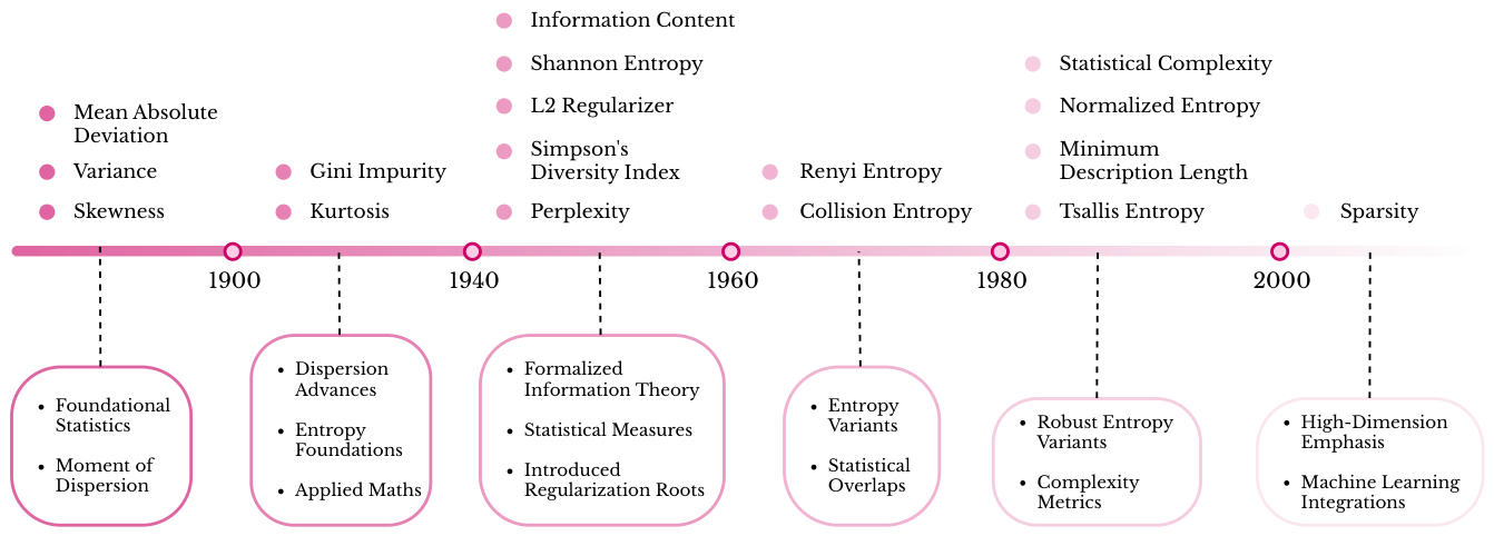
Figure 3.
Taxonomy of the surveyed objectives grouped into information-theoretic, probabilistic dispersion, geometric distribution, and regularization families.
Figure 3.
Taxonomy of the surveyed objectives grouped into information-theoretic, probabilistic dispersion, geometric distribution, and regularization families.
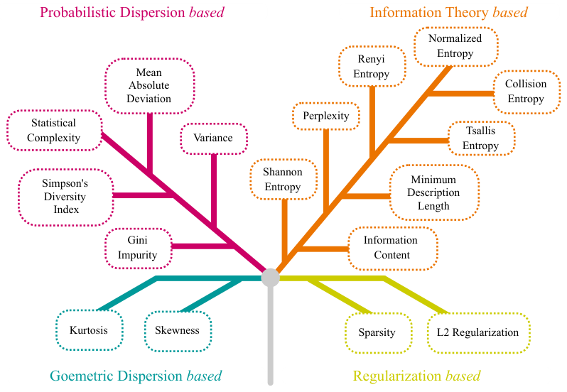
Figure 8.
Confusion Matrix of 4x datasets for ResNet-18 when optimized with Shannon Entropy (Eq. 4). Optimizing with Shannon Entropy leads to consistent predictions and improved performance.
Figure 8.
Confusion Matrix of 4x datasets for ResNet-18 when optimized with Shannon Entropy (Eq. 4). Optimizing with Shannon Entropy leads to consistent predictions and improved performance.
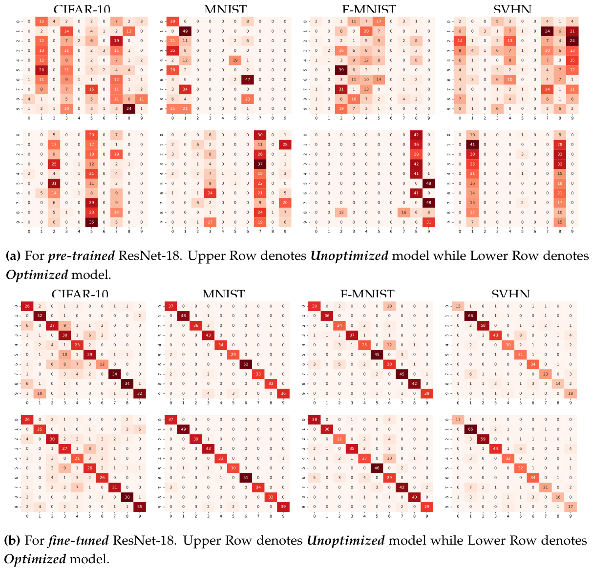
Figure 9.
Confusion Matrix of 4x datasets for ResNet-18 when optimized with Information Content (Eq. 11). Optimizing with Information Content leads to inconsistencies in predictions and thus degraded performance.
Figure 9.
Confusion Matrix of 4x datasets for ResNet-18 when optimized with Information Content (Eq. 11). Optimizing with Information Content leads to inconsistencies in predictions and thus degraded performance.
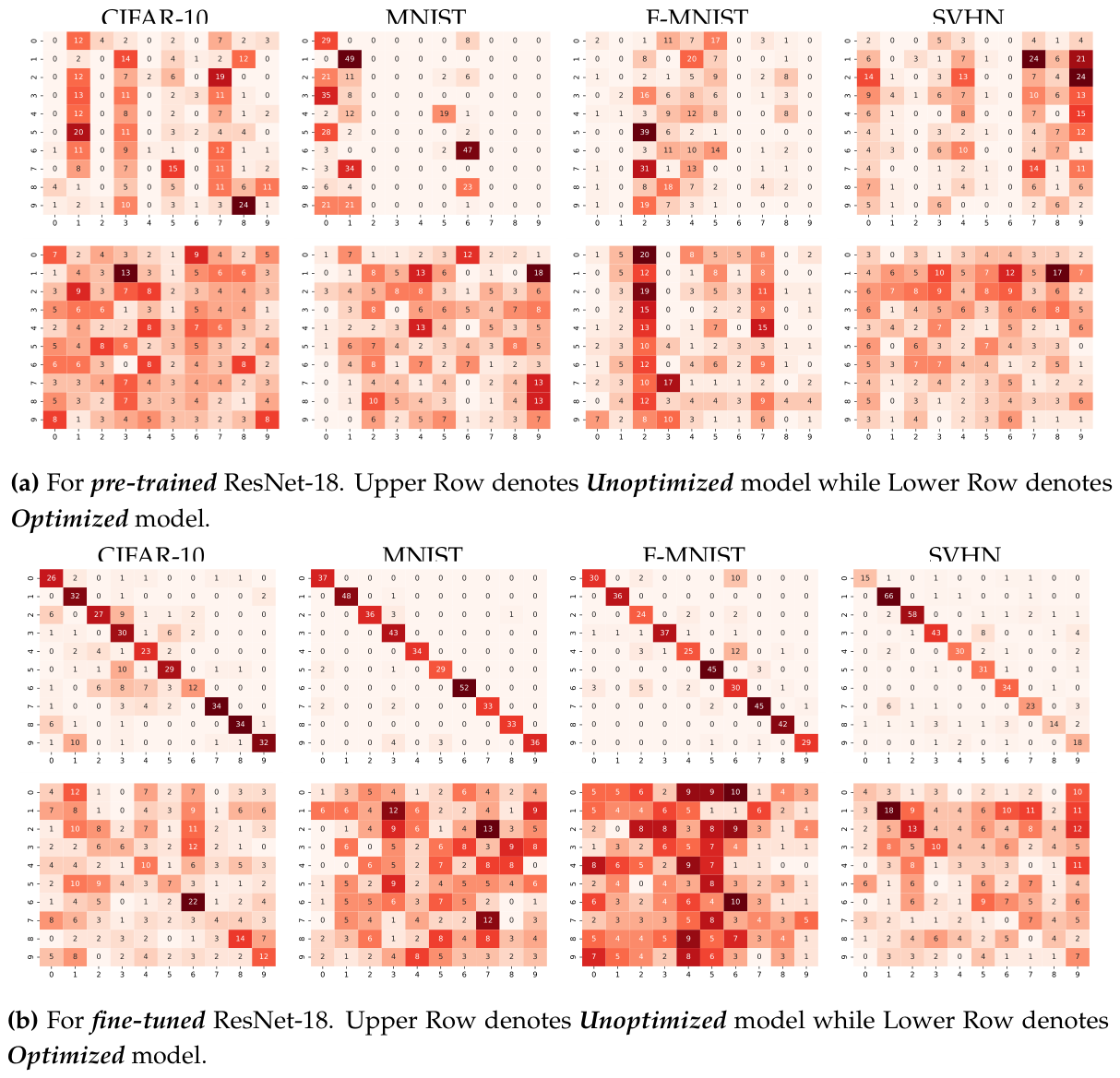
Figure 10.
Pairwise comparison for 8 information theory-based unsupervised loss functions. Each subplot shows the relationship between two metrics, capturing their joint behavior. Diagonal subplots represent the self-comparison of each metric, while off-diagonal subplots illustrate the inter-metric correlations.
Figure 10.
Pairwise comparison for 8 information theory-based unsupervised loss functions. Each subplot shows the relationship between two metrics, capturing their joint behavior. Diagonal subplots represent the self-comparison of each metric, while off-diagonal subplots illustrate the inter-metric correlations.
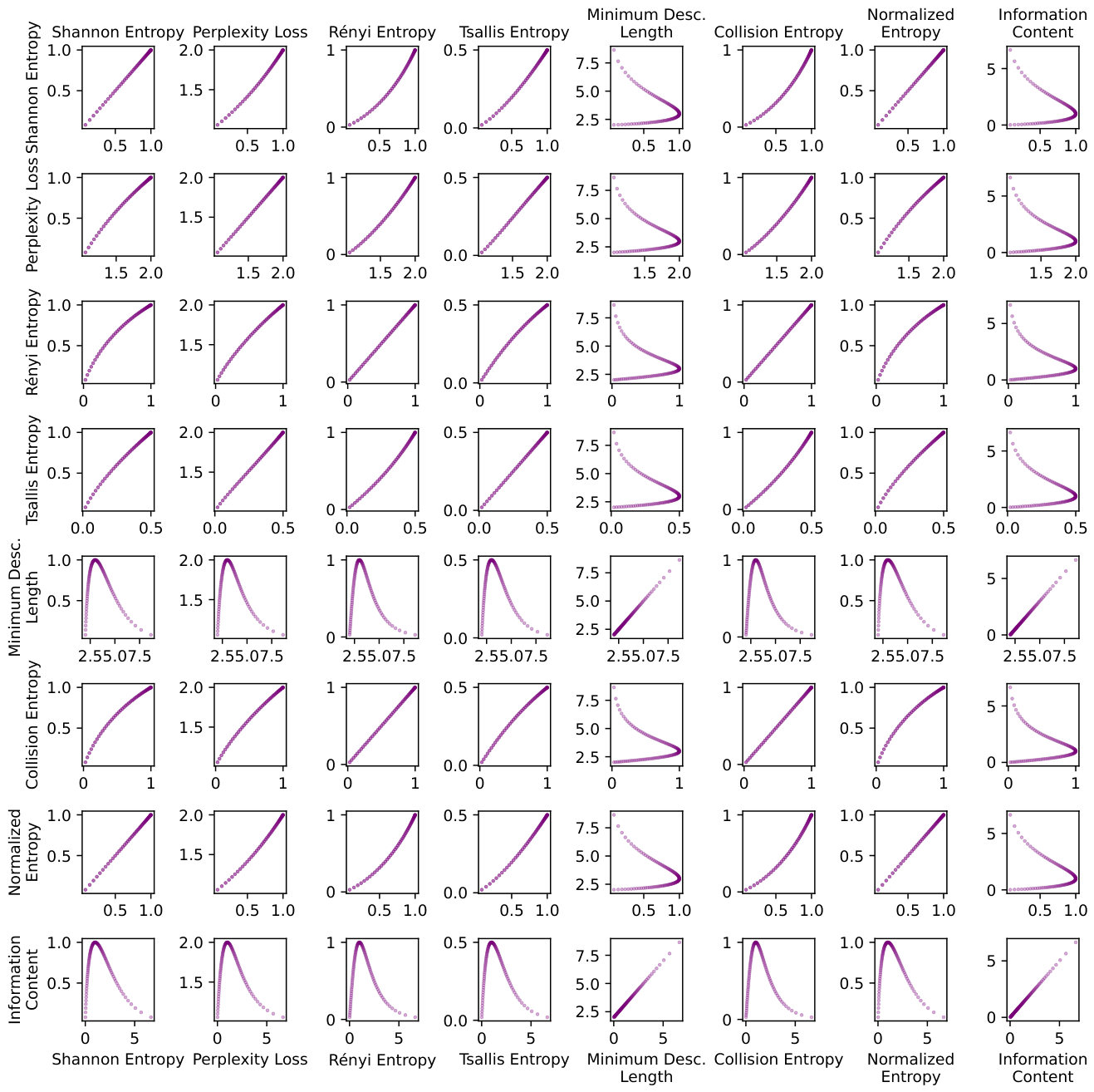
Figure 11.
Pairwise comparison matrices illustrating inter-metric behaviour for the two groups of unsupervised objectives ((a): probabilistic-dispersion; (b): geometric + regularization based objectives). (Zoom in for clarity).
Figure 11.
Pairwise comparison matrices illustrating inter-metric behaviour for the two groups of unsupervised objectives ((a): probabilistic-dispersion; (b): geometric + regularization based objectives). (Zoom in for clarity).
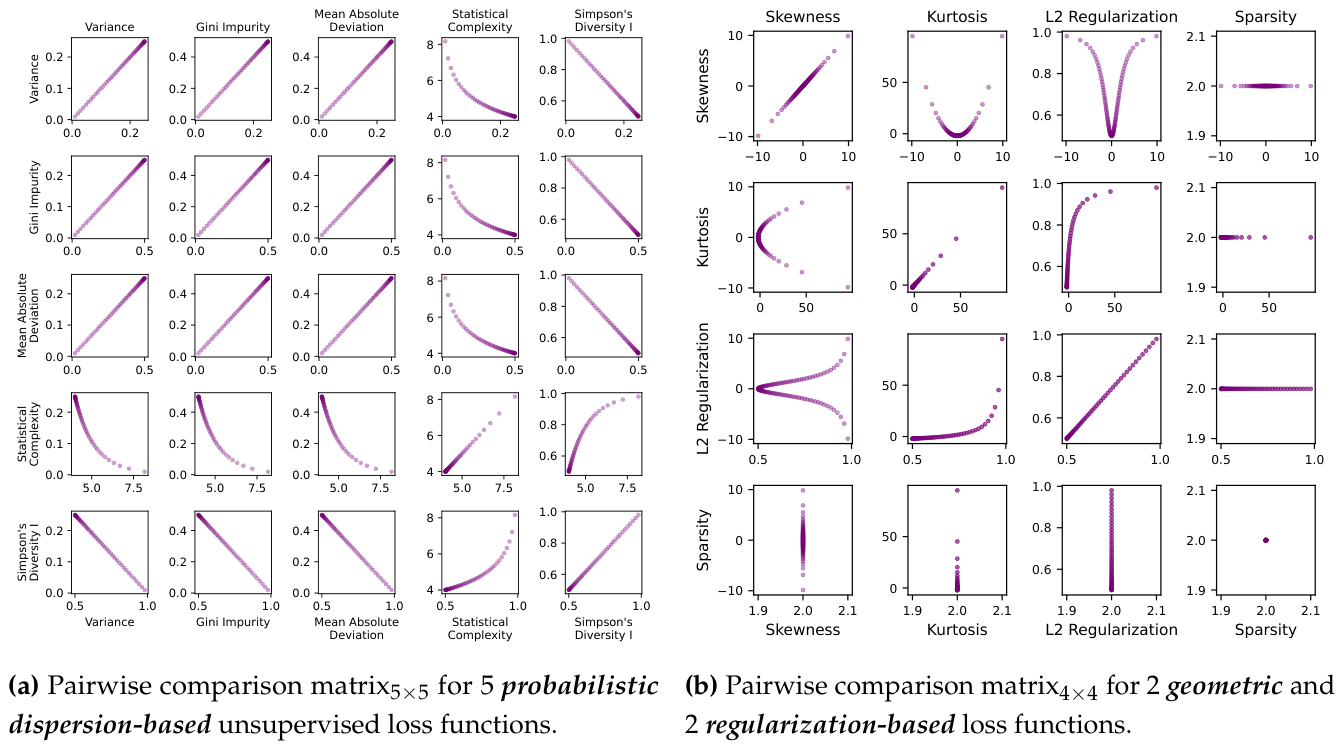
Figure 12.
Rate of change analysis for 17 unsupervised objectives as a function of probability (P). Each subplot represents the first derivative () and second derivative () of the respective function, highlighting the zero-crossing points. Zero-crossing points are annotated, indicating critical points where the rate of change transitions.
Figure 12.
Rate of change analysis for 17 unsupervised objectives as a function of probability (P). Each subplot represents the first derivative () and second derivative () of the respective function, highlighting the zero-crossing points. Zero-crossing points are annotated, indicating critical points where the rate of change transitions.
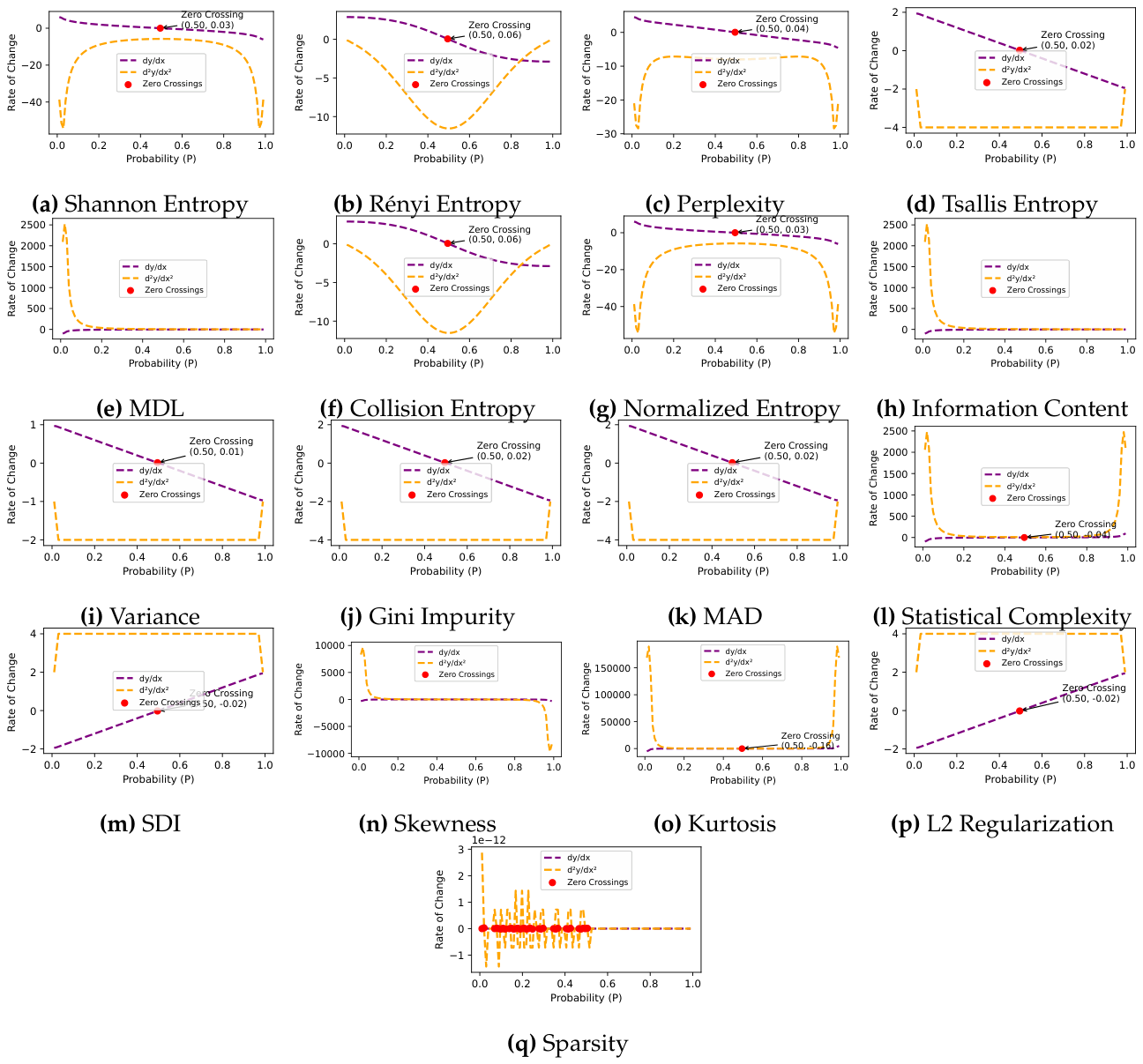
Table 5.
Comparison of the performance of the initially unoptimized Base model with 17 optimized models when optimized using unsupervised loss functions. In this configuration, ResNet-18 was initialized with ImageNet pre-trained weights. F-MNIST refers to Fashion MNIST, while Average represents the mean performance across all 4 datasets. Green and Red indicate whether the performance of the optimized models is higher or lower than Base, respectively. Results represent the mean across 3 runs with different seeds.
Table 5.
Comparison of the performance of the initially unoptimized Base model with 17 optimized models when optimized using unsupervised loss functions. In this configuration, ResNet-18 was initialized with ImageNet pre-trained weights. F-MNIST refers to Fashion MNIST, while Average represents the mean performance across all 4 datasets. Green and Red indicate whether the performance of the optimized models is higher or lower than Base, respectively. Results represent the mean across 3 runs with different seeds.
| Dataset → | ImageNet Pre-Trained Initialized | ||||
|---|---|---|---|---|---|
| Loss Function ↓ | CIFAR-10 | MNIST | F-MNIST | SVHN | Average |
| Base | 9.42 ± 3.19 | 9.83 ± 1.43 | 9.42 ± 2.00 | 9.17 ± 1.98 | 9.46 ± 2.15 |
| 1. Shannon Entropy [Eq. 4] | 9.58 ± 2.28 | 14.00 ± 12.46 | 13.08 ± 4.09 | 11.00 ± 1.97 | 11.92 ± 5.20 |
| 2. Perplexity [Eq. 5] | 7.42 ± 3.50 | 16.25 ± 4.10 | 8.58 ± 3.86 | 11.67 ± 1.12 | 10.98 ± 3.15 |
| 3. Renyi Entropy [Eq. 6] | 10.17 ± 5.80 | 11.33 ± 3.86 | 8.3 ± 0.62 | 10.58 ± 0.77 | 10.10 ± 2.76 |
| 4. Tsallis Entropy [Eq. 7] | 9.08 ± 4.70 | 14.58 ± 6.49 | 11.00 ± 0.94 | 9.58 ± 2.66 | 11.06 ± 3.70 |
| 5. MDL [Eq. 8] | 7.33 ± 1.65 | 11.17 ± 3.60 | 9.75 ± 1.54 | 9.08 ± 1.25 | 9.33 ± 2.01 |
| 6. Collision Entropy [Eq. 9] | 13.00 ± 5.81 | 10.50 ± 4.34 | 8.50 ± 4.43 | 11.42 ± 1.05 | 10.86 ± 3.91 |
| 7. Normalized Entropy [Eq. 10] | 10.08 ± 3.94 | 3.67 ± 1.93 | 7.42 ± 5.37 | 7.33 ± 1.01 | 7.13 ± 3.06 |
| 8. Information Content [Eq. 11] | 9.75 ± 0.71 | 9.67 ± 0.82 | 8.00 ± 1.59 | 8.33 ± 0.82 | 8.94 ± 0.99 |
| 9. Variance [Eq. 12] | 12.75 ± 6.56 | 12.25 ± 7.18 | 9.58 ± 2.18 | 15.33 ± 0.96 | 12.48 ± 4.22 |
| 10. Gini Impurity [Eq. 13] | 15.25 ± 6.45 | 14.08 ± 6.80 | 12.00 ± 6.29 | 9.17 ± 1.96 | 12.63 ± 5.38 |
| 11. MAD [Eq. 14] | 11.17 ± 1.36 | 12.33 ± 4.73 | 9.75 ± 6.84 | 10.25 ± 1.02 | 10.88 ± 3.49 |
| 12. Statistical Complexity [Eq. 15] | 9.83 ± 0.72 | 7.25 ± 3.59 | 9.33 ± 1.03 | 11.25 ± 0.74 | 9.42 ± 1.52 |
| 13. SDI [Eq. 16] | 9.50 ± 0.54 | 10.33 ± 1.01 | 11.08 ± 0.12 | 10.08 ± 1.65 | 10.25 ± 0.83 |
| 14. Skewness [Eq. 17] | 8.75 ± 0.20 | 10.33 ± 2.05 | 9.33 ± 3.63 | 11.58 ± 1.18 | 10.00 ± 1.77 |
| 15. Kurtosis [Eq. 18] | 8.67 ± 1.50 | 9.83 ± 2.18 | 11.92 ± 3.03 | 9.50 ± 1.74 | 9.98 ± 2.11 |
| 16. Regularization [Eq. 19] | 10.25 ± 1.41 | 10.08 ± 2.97 | 8.00 ± 1.06 | 9.67 ± 0.66 | 9.50 ± 1.53 |
| 17. Sparsity [Eq. 20] | 8.25 ± 1.34 | 11.08 ± 3.55 | 9.42 ± 0.94 | 9.42 ± 1.05 | 9.54 ± 1.72 |
Table 6.
Comparison of the performance of the initially unoptimized Base model with 17 optimized models when optimized using unsupervised loss functions. In this configuration, ImageNet initialized ResNet-18 was fine-tuned on each downstream dataset. F-MNIST refers to Fashion MNIST, while Average represents the mean performance across all 4 datasets. Green and Red indicate whether the performance of the optimized models is higher or lower than Base, respectively. Results represent mean across 3 runs with different seeds.
Table 6.
Comparison of the performance of the initially unoptimized Base model with 17 optimized models when optimized using unsupervised loss functions. In this configuration, ImageNet initialized ResNet-18 was fine-tuned on each downstream dataset. F-MNIST refers to Fashion MNIST, while Average represents the mean performance across all 4 datasets. Green and Red indicate whether the performance of the optimized models is higher or lower than Base, respectively. Results represent mean across 3 runs with different seeds.
| Dataset → | Fine-Tuned on Downstream Task | ||||
|---|---|---|---|---|---|
| Loss Function ↓ | CIFAR-10 | MNIST | F-MNIST | SVHN | Average |
| Base | 65.17 ± 1.50 | 96.00 ± 1.43 | 83.25 ± 0.82 | 83.42 ± 1.59 | 81.79 ± 1.64 |
| 1. Shannon Entropy [Eq. 4] | 67.92 ± 2.87 | 97.33 ± 0.85 | 84.08 ± 1.76 | 83.33 ± 0.66 | 83.17 ± 1.54 |
| 2. Perplexity [Eq. 5] | 68.58 ± 1.16 | 96.92 ± 0.31 | 84.00 ± 0.54 | 85.00 ± 1.14 | 83.63 ± 0.79 |
| 3. Renyi Entropy [Eq. 6] | 71.17 ± 1.93 | 97.25 ± 0.71 | 84.25 ± 1.74 | 87.50 ± 0.35 | 85.04 ± 1.18 |
| 4. Tsallis Entropy [Eq. 7] | 68.50 ± 1.59 | 96.67 ± 0.85 | 85.58 ± 0.51 | 85.75 ± 0.61 | 84.13 ± 0.89 |
| 5. MDL [Eq. 8] | 15.58 ± 1.76 | 12.83 ± 3.51 | 14.42 ± 1.43 | 13.42 ± 2.86 | 14.06 ± 2.39 |
| 6. Collision Entropy [Eq. 9] | 69.25 ± 1.14 | 97.00 ± 1.22 | 84.67 ± 0.62 | 83.08 ± 1.64 | 83.50 ± 1.16 |
| 7. Normalized Entropy [Eq. 10] | 68.42 ± 1.43 | 96.75 ± 0.54 | 86.00 ± 1.43 | 84.42 ± 1.90 | 83.90 ± 1.33 |
| 8. Information Content [Eq. 11] | 21.83 ± 3.26 | 12.08 ± 2.32 | 17.00 ± 2.35 | 15.33 ± 3.48 | 16.56 ± 2.85 |
| 9. Variance [Eq. 12] | 66.75 ± 1.08 | 96.00 ± 0.35 | 85.25 ± 0.54 | 84.58 ± 1.36 | 83.15 ± 0.83 |
| 10. Gini Impurity [Eq. 13] | 68.83 ± 1.74 | 96.33 ± 0.12 | 83.92 ± 1.65 | 84.08 ± 1.16 | 83.29 ± 1.17 |
| 11. MAD [Eq. 14] | 67.75 ± 3.69 | 96.33 ± 1.83 | 87.25 ± 0.74 | 85.42 ± 0.66 | 84.19 ± 1.73 |
| 12. Statistical Complexity [Eq. 15] | 72.92 ± 0.51 | 97.50 ± 0.74 | 85.17 ± 1.20 | 85.50 ± 2.07 | 85.27 ± 1.13 |
| 13. SDI [Eq. 16] | 21.92 ± 2.00 | 12.42 ± 1.85 | 15.83 ± 5.29 | 21.67 ± 4.40 | 17.96 ± 3.39 |
| 14. Skewness [Eq. 17] | 53.58 ± 2.35 | 63.08 ± 19.93 | 52.17 ± 5.33 | 65.83 ± 3.86 | 58.67 ± 7.87 |
| 15. Kurtosis [Eq. 18] | 63.67 ± 1.74 | 94.17 ± 2.79 | 74.50 ± 4.22 | 76.00 ± 3.02 | 77.09 ± 2.94 |
| 16. Regularization [Eq. 19] | 31.25 ± 0.71 | 8.00 ± 3.61 | 18.25 ± 3.36 | 17.92 ± 1.66 | 18.86 ± 2.34 |
| 17. Sparsity [Eq. 20] | 73.17 ± 0.62 | 98.00 ± 0.74 | 86.33 ± 1.93 | 84.50 ± 1.43 | 85.50 ± 1.18 |
Disclaimer/Publisher’s Note: The statements, opinions and data contained in all publications are solely those of the individual author(s) and contributor(s) and not of MDPI and/or the editor(s). MDPI and/or the editor(s) disclaim responsibility for any injury to people or property resulting from any ideas, methods, instructions or products referred to in the content. |
© 2026 by the authors. Licensee MDPI, Basel, Switzerland. This article is an open access article distributed under the terms and conditions of the Creative Commons Attribution (CC BY) license (http://creativecommons.org/licenses/by/4.0/).
Copyright: This open access article is published under a Creative Commons CC BY 4.0 license, which permit the free download, distribution, and reuse, provided that the author and preprint are cited in any reuse.