

Submitted:
02 June 2026
Posted:
04 June 2026
You are already at the latest version
Abstract
In this study, we introduce idempotent Neutrosophic Hypersoft Rough Fuzzy Matrices (INHSRFMs) and focus on a particular case, the INHSRFM of T-type. We derive various properties for both INHSRFM and INHSRFM of T-type and present a series of theorems that validate our results. To illustrate the application of these theorems, a numerical example is included. Additionally, we propose an algorithm designed to solve decision-making (DM) problems using NHSRFMs. The practical applicability of the proposed method is demonstrated through an example.
Keywords:
neutrosophic fuzzy sets
; neutrosophic fuzzy matrices
; idempotent neutrosophic hypersoft rough fuzzy matrices of T-type
1. Introduction
The notion of Fuzzy Set (FS), presented by Zadeh [1], has played a crucial role in addressing uncertainty across various domains, including decision making and system modeling. Building upon this concept, Atanassov expanded FS theory by introducing Intuitionistic FS (IFS) which not only represent membership but also include an independent degree of non-membership, providing a more versatile way to model uncertainty [2]. To account for higher levels of uncertainty, Smarandache proposed the Neutrosophic Set (NS) [34] , a generalization of the IFSs [2]. Details development and applications of NSs were studied by several researchers [38,39]. Neutrosophic matrices, which capture ( T, I, F ) have become essential in developing new matrix forms that enable more detailed analysis.
Research has since progressed in refining and applying these concepts. Jang et al. [3] examined the distances between interval-valued IFSs, a key contribution to understanding the relationships between different fuzzy sets in complex systems. Park et al. [4] developed a generalized IFSs approach, applying this theory to decision making problems. Further advancements were made by Kim and Roush, who introduced generalized Fuzzy matrix( FM), expanding the scope of FS theory in matrix operations [5].
Thomason’s work on the convergence of powers of FM paved the way for deeper analysis of matrix behaviours under fuzzy conditions [6], while Kim [7] studied idempotents and inverses in fuzzy matrices, offering valuable insights into the structural properties of FMs. Mishref and Emam contributed to understanding the transitivity and sub inverses within FMs, which is crucial for the analysis of relations in fuzzy systems [8]. Additionally, Ragab and Emam’s work on the determinant and adjoint of FM provided essential algebraic tools for further exploration [9].
The study of intuitionistic FM (IFM), as explored by Pal [12] and others, has led to significant theoretical developments, including the concept of Intuitionistic Fuzzy (IF) determinants [12], the adjoint of IFM [13], and the introduction of new operators on FMs by Shyamal and Pal [15]. Furthermore, generalized IFMs, as studied by Bhowmik and Pal, have led to new insights in matrix theory and their applications in decision making [17,18].
In recent years, researchers like Khan and Pal [20] have explored the generalized inverse of IFM, while Adak et al. [21] examined properties of generalized nilpotent IFM. The development of the max-max operation on IFM by Padder and Murgadas [22], and the reduction of intuitionistic fuzzy rectangular matrices [23], reflect the ongoing efforts to extend the applicability of intuitionistic fuzzy matrices in computational systems and decision-making frameworks.
One of the foundational concepts in this field is the study of fuzzy idempotent matrices, which are crucial in understanding the behaviour and properties of matrices under fuzziness. Kim [10] explored this concept, focusing on FIM of T-type and their applications in information sciences. Additionally, Meenakshi [11] provided an extensive discussion on the theory and applications of fuzzy matrices, offering valuable insights into their mathematical framework. Further advancements were made in the realm of intuitionistic fuzzy matrices, with several researchers delving into their theoretical aspects. Notably, Pal, Khan, and Shyamal [14] introduced IFM, while Shyamal and Pal [16] studied the distance metrics between these matrices. The study of generalized interval-valued IFSs by Bhowmik and Pal [19] expanded the scope of fuzzy systems, highlighting their potential in handling more complex uncertainty.
Pradhan and Pal [24] examined the convergence of various operations, such as max-arithmetic and min-arithmetic means, in the context of IFM. Sriram and Murugadas [25] further advanced the field by studying the semirings and sub-inverses of IFM, providing key results in the algebraic structure of these matrices. Sriram and Murugadas [26] also explored sub-inverses, deepening the understanding of matrix inverses within the intuitionistic fuzzy framework. Lee and Jeong [27] presented canonical form of transitive IFM, which has implications for their practical applications. The work of Atanassov [28] on generalized index matrices and IFS laid the groundwork for many of these advancements, influencing both the theoretical and practical development of fuzzy matrix theory. Furthermore, research into the adjoint of square IFM, as explored by Im, Lee, and Park [30], provided important results related to the computational aspects of these matrices. These contributions collectively underscore the growing importance and versatility of IFM in various branches of mathematics and their applications in real-world problems.
The idea of IFM was examined by Padder and Murugadas [31], who focused on the idempotency of IFM of T-type, demonstrating how such matrices can be applied in fuzzy decision-making scenarios. Uma et al. explored this concept further by developing determinant theory for fuzzy NSM, providing a basis for new computational methods [32]. Their subsequent work delved into Type I and Type II fuzzy NSM, which offer enhanced flexibility in decision-making models [33]. More recently, advancements have been made in understanding the structural properties of neutrosophic matrices. Anandhkumar et al. [35] studied k-idempotent HSRFM, contributing new insights into their partial ordering and characterizations. They further explored pseudo similarity in neutrosophic fuzzy matrices, establishing essential criteria for comparing these matrices under various transformations [36].
1.1. Abbreviations and notations
FM: Fuzzy Matrices
FIM: Fuzzy Idempotent Matrices
MCDMP: Multi-Criteria Decision- Making Problem.
P = PT: Symmetric
: (Max-min) transitive
: Nilpotent
P = P2: Idempotent
2. The Organization of this Paper Is Presented as Follows
Section 3 reviews literature on NHSRFMs, focusing on their evolution, properties, and applications. Section 4 identifies research gaps, emphasizing the need for enhanced NHSRFM models. Section 5 highlights our main contributions, Section 6 highlights a novel NHSRFM model with unique properties like idempotency and normality and compares our model to existing soft computing approaches, underscoring its strengths in handling uncertainty. Section 7 covers preliminaries and foundational concepts and introduces idempotent NHSRFMs Section 8 explores properties of idempotent and normal HSRFMs. Section 9 further examines properties of NHSRFMs with idempotent, normal, and T-type characteristics. Section 10 presents an algorithm based on NHSRFMs, with Section 11 demonstrating it through a practical example. Section 12 concludes with insights and future research directions, reinforcing the model?s potential applications and areas for further study.
3. Literature Review
The foundational work on FSs was presented by Zadeh [1], laying the groundwork for FM. Atanassov’s introduction of IFS [2] further expanded the scope, allowing for the consideration of ( T, I, F ). in decision-making problems.
Fuzzy and IFM
Kim [7] and Mishref & Emam [8] explored key concepts of FMs, particularly focusing on idempotency and inverse properties. These studies provided the groundwork for the subsequent development of idempotent fuzzy. Further contributions by Pal [12] and Shyamal & Pal [15] expanded these ideas to IFM, addressing concepts such as determinants and new matrix operations. The properties of generalized fuzzy matrices were also investigated by Kim & Roush [5], where fuzzy operations were generalized to handle more complex cases.
In the context of IFM, the work by Pal et al. [14] and Im et al. [13] focused on determinants and adjoint matrices. The concept of the adjoint of IFM was further developed by Im et al. [30], offering valuable insights into the structural properties and operational results of IFM. Padder and Murugadas [31] extended this work by introducing idempotent IFM of T-type, offering a more generalized approach to decision-making scenarios.
Neutrosophic Fuzzy Matrices
The notion of IFS, introduced by Smarandache [34], extends IFS by incorporating three components ( T, I, F ). This has led to the development of HSRFMs, which capture more complex forms of uncertainty and inconsistency in data. Uma, Murugadas, and Sriram [32] introduced determinant theory for IFM, expanding the theoretical framework to include more general forms of fuzzy matrices. Further exploration of fuzzy NSM of Type I and Type II [33] provided additional tools for handling DM problems in uncertain environments.
Recent Developments in Idempotent Neutrosophic Fuzzy Matrices
Recent studies have focused on the idempotency property in the context of HSRFM. Anandhkumar et al. [35] explored the generalization of k-idempotent HSRFM, contributing to a deeper understanding of matrix operations under uncertainty. Anandhkumar, Kamalakannan, and Chithra [36] further explored pseudo-similarity of neutrosophic fuzzy matrices, an important concept for comparing matrices in DM problems.
Gap in the Literature and Motivation for the Current Work
While the literature on idempotent fuzzy matrices and intuitionistic fuzzy matrices is rich, there remains a lack of comprehensive studies on idempotent neutrosophic fuzzy matrices of T-type. Most existing work focuses on either intuitionistic fuzzy or neutrosophic fuzzy matrices separately, with limited attention paid to combining these concepts in the context of DM problems. Therefore, the present work seeks to address this gap by developing a more generalized framework for idempotent NHSRFM of T-type and exploring their application in MCDM.
Summary of Key Contributions:
- NFM: Smarandache’s neutrosophic set theory [34] extended fuzzy logic to include indeterminacy and falsity, impacting matrix theory.
4. Research Gap
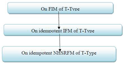
Previous studies, such as those by Kim [10] on FIM of T-Type and by Riyaz Ahmad Padder et al. [31] on idempotent IFM of T-Type, have contributed to the foundational understanding of idempotent matrices within fuzzy and intuitionistic fuzzy contexts. However, these approaches are limited in handling indeterminate and inconsistent information. NHSRFM, with their capacity to incorporate truth, indeterminacy, and falsity, offer a more comprehensive framework, yet their idempotent forms, specifically of T-Type, remain unexplored. To address this research gap, We have developed this article and also examined their application to MCDM.

Table 1.
An overview of the research progress in extending NHSRFM.
| References | Extension of NHSRFM. | Year |
| Kim [10] | On fuzzy idempotent matrices of T-Type | 1994 |
| Padder [31] | On idempotent IFM of T-Type | 2016 |
| Proposed | Algebraic Properties of Idempotent Neutrosophic Hypersoft Rough Fuzzy Matrices of T-Type | 2026 |
5. Main Contribution of Our Work
- (a)
- Investigate Idempotent Neutrosophic Hypersoft Rough Fuzzy Matrices (NHSRFMs): To explore the properties and characteristics of idempotent NHSRFMs, with a focus on their mathematical structure and behavior.
- (b)
- Examine Idempotent Neutrosophic Hypersoft Rough Fuzzy Matrices of T-type: To study the specific case of idempotent NHSRFMs of T-type and establish their properties within the broader framework of NHSRFMs.
- (c)
- Develop Theoretical Results: To formulate and prove a set of theorems that offer a deeper kind of the properties of idempotent NHSRFMs and their applications.
- (d)
- Provide Numerical Validation: To present a numerical illustration that illustrates the application and validity of the established theorems, demonstrating the theoretical findings in a practical context.
- (e)
- Design a Decision-Making Algorithm: To develop an algorithm that utilizes NHSRFMs to address multi-criteria decision-making (MCDM) problems, especially those involving uncertainty and indeterminacy.
6. Novelty
The foundational concepts of FSs, presented by Zadeh [1], laid the groundwork for handling uncertainty in mathematical frameworks. Building on this, Atanassov [2] extended fuzzy sets to IFM, incorporating an additional layer of hesitation, which has since become pivotal in various fields. Further, interval-valued IFS [3] and generalized IFSS, [4] offer a refined approach to capturing uncertainties in complex decision-making contexts.
The application of matrix theory to fuzzy logic began with Kim and Roush’s exploration of generalized fuzzy matrices [5], followed by Thomason’s work on the convergence of powers in fuzzy matrices [6]. Over the years, studies have delved into idempotency [7], transitivity [8], and determinant properties [9] of fuzzy matrices, with subsequent research expanding these concepts to intuitionistic fuzzy matrices. For instance, Kim [10] examined idempotent intuitionistic fuzzy matrices, which are useful for stability analysis in systems with fuzziness, while Pal [12] introduced the intuitionistic fuzzy determinant, further explored by Im, Lee, and Park [13] in square intuitionistic fuzzy matrices.
Recent work on neutrosophic fuzzy matrices has significantly extended these concepts. Smarandache’s NS theory [34] generalizes IFSs by integrating indeterminacy, thus allowing for more nuanced decision models. Foundational contributions to fuzzy neutrosophic matrices were done in the studies [32,33] which established determinant theory and defined Type I and Type II classifications, respectively. Their work enables the application of fuzzy neutrosophic matrices in fields requiring multi-dimensional uncertainty analysis.
Anandhkumar and colleagues [35] introduced k-idempotent neutrosophic fuzzy matrices, detailing partial orderings and characterizations that enhance matrix-based comparison frameworks. Further, Anandhkumar et al. [36] introduced pseudo similarity for neutrosophic fuzzy matrices, providing a unique perspective on matrix equivalency. These studies represent progressive steps in adapting fuzzy and neutrosophic matrix frameworks to handle varying levels of uncertainty, complexity, and indeterminacy, underscoring their value in modern decision-support applications.
7. Preliminaries, Idempotent NHSRFM
Presented below are several key definitions and outcomes utilized in this paper
Definition:7.1 Let P and Q be an n x n NHSRFMs where and respectively. We define the following for upper NHSRFMs
(i)
(ii)
(iii)
(iv)
Definition:7.2 Idempotent NHSRFMs
An idempotent NHSRFMs P satisfies the condition: P2 = P
Example:7.1 Let us consider 3x3 Upper NHSRFMs
Definition:7.3 A NHSRFMs P is lease than or equal to Q
That is if means .
Example:7.2 Let us consider 3x3 Upper NHSRFMs
Definition:7.4 Let P is defined as normal if .
Example:7.3 Let us consider 3x3 Upper NHSRFM
Therefore,
8. Properties of Idempotent and Normal NHSRFMs
Theorem:8.1 Let be an idempotent NHSRFMs. If P is normal, then
for every belongs to .
(i) Let
If then there exist or such that or
Proof: (i) In order to prove
we have to first show that .
Suppose that (we shall obtain contradiction).
Put
The proof proceeds with the following steps
(a) Since P is idempotent, meaning P2 = P, we have that and
for 1< k< n.
If k =1, Subsequently
Contrary to
In a similar way, we can show that
If
Contrary to
We get,
and
(b) Suppose that is the first such element from with property
and not exists such that 1 < t < k .
Note that
Since PP = P, for there exists such that
= and
We assume that is the initial one from with this property.
If u = k, then , which is contradicts
Thus, we get k < u. If u = n,
But we know that from that
Then we obtain that , contradicts with
. We say that
with k<u<n.
(c) Following the argument presented above for ,
We get that
with 1<k<u<v<n.
If v = u, subsequently
contradicts to
and
(if v = n, then
and
and
Then we take PT and using the above statement, we have for t = n-1, n-2,…,2
(ii) Let with and
Then we see that
and
We also see that
and
Thus, we get
which reduce that
or
This prove (ii)
Hence the theorem.
Example:8.1 Let us consider 3x3 Upper NHSRFM
Let P is Idempotent and P is normal
Then for every belongs to .
All the elements of the matrix above is less then or equal to . Therefore (i) is true.
Let
If then there exist or such that or
If
then there exist or such that or .
9. Properties of Idempotent, Normal and T-Type NHSRFMs
Definition:9.1 (a) Let denote the determinant of P. (b) adj(P) = Q = represent the adjoint matrix of P, well-defined as follows:
and is the (n-1) x(n-1) NHSRFM obtained by removing row j and column i from matrix P.
(c) Let be an idempotent NHSRFM, and assume that P is normal. P is said to be T-type if
for
ie, and
and for
i.e, and .
Example:9.1 Let us consider 3x3 Upper NHSRFM
Theorem:9.1 Let be a idempotent matrix of T-type, and assume that P is normal. Then adj(P) is an idempotent NHSRFM.
Example:9.2 Let assume that Upper 3x3 NHSRFM
Therefore, P is an idempotent NHSRFM of the T-type and also P is normal.
Now,
Therefore, Q is also an idempotent NHSRFM
10. Algorithm for Decision-Making Using NHSRFM
Definition 10.1. Let Y = {y1, y2,.....,yn} be a universe set and E = {e1,e2,.....,em} be a set of restrictions. Then, for an NHSRFM (,E) over Y the degree of TM, degree of IM and degree of FM of an element yi to (ej) denoted by , and correspondingly. Then, the corresponding score functions are represented and formulated as follows:
and
Definition 10.2. Let X = {y1, y2, ....., yn} be a universe set and E = {e1, e2 ,....., em} be a set of parameters. For an NHSRFM (,E) over Y, the scores of the TM, IM and FM of yi for each ej be denoted by, and correspondingly. Then, the total score of xi for each ej is represented by
Based on the above definitions, the procedure of the proposed algorithm (see Figure 1) is described through the following steps:
Algorithm:
Step 1. For the universal set Y = {y1, y2, …, yn} and the parameter set E = {e1, e2, …, em} input the matrix representation of an NHSRFM (,E) in tabular form, according to a decision-maker.
Step 2. With reference to the input matrix constructed in Step 1, and by applying Definitions 10.1 and 10.2, the corresponding computations are carried out as follows: We calculate , , and for xi for each ej where i = 1 to n; j = 1 to m.
Step 3. Using the values obtained in Step 2 and applying Definition 11.3, the following results are determined: We calculate the score of xi for each ejwhere i = 1 to n; j = 1 to m.
Step 4. Calculate the overall score vi for xiin such a way that
Step 5. Find k, for which vk = maxxi∈X{vi}. Then, xk ∈ X is the best choice.
Step 6. If a tie occurs among the alternatives, both alternatives may be considered as optimal choices. Alternatively, the decision-makers may review the evaluations with the guidance of experts, revise the values if necessary, and repeat the previous steps of the procedure to obtain a final decision.
11. To Demonstrate the Practical Application of the Algorithm, We Present the Following Example
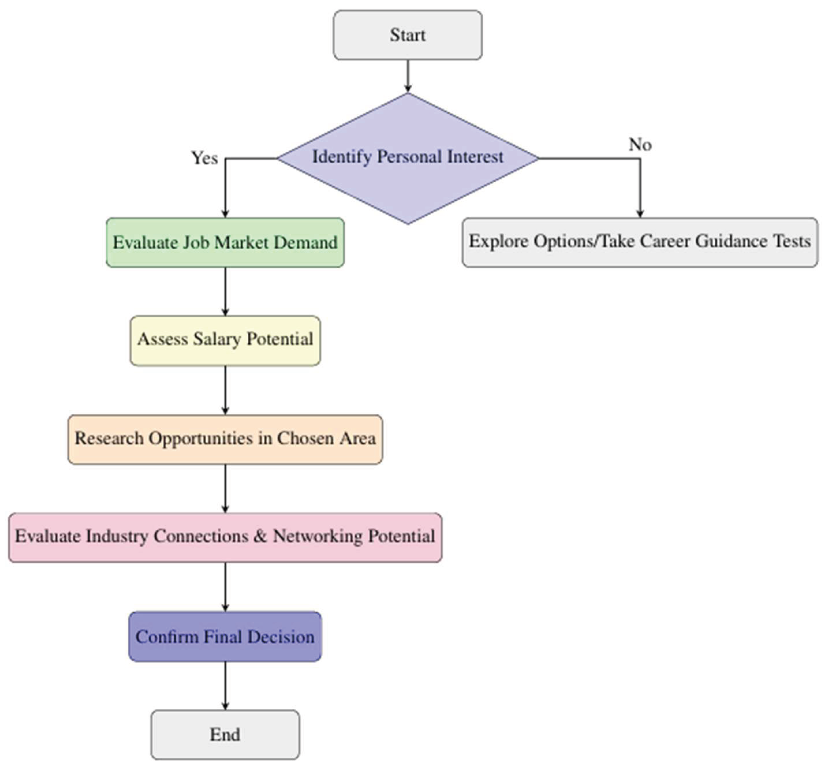
Example 11.1. To effectively implement the proposed algorithm in a practical scenario, we face a specific challenge: imagine an individual seeking to choose one engineering course from a pool of five distinct options. This decision-making process is particularly complex due to the individual’s limited knowledge and understanding of how to identify a suitable course. Several conflicting factors come into plays that further complicate the selection. To navigate this intricate decision-making landscape, the individual sought guidance from a group of experts and DMs with backgrounds in engineering. These specialists possess valuable insights and experience, allowing them to meticulously evaluate the five courses based on established criteria. The evaluation process is carried out methodically to ensure a thorough comparison of the alternatives. Each course is assessed according to various factors, which may include curriculum content, faculty expertise, career outcomes, and student satisfaction. By synthesizing the expert evaluations, the aim is to identify the most suitable course (See Figure 2) that aligns with the individual’s educational and career aspirations, thus facilitating a more informed and confident decision.
Step 1. Step 1: Let the collection of engineering courses be represented as Y = {y1, y2, y3, y4, y5} and let the set of evaluation criteria E = {ei: i = 1,2,3,4,5},
To evaluate these courses within a MCDM background. Based on your choice, here are five applicable parameters
e1: Job Market Demand (Weight: 30 percentage) – The current and projected demand for professionals in each field, indicating employability.
e2: Salary Potential (Weight: 25 percentage) – The average starting salary and potential earning power in each field.
e3: Research Opportunities (Weight: 20 percentage) – Availability and quality of research and innovation opportunities in each field.
e4: Industry Connections (Weight: 15 percentage) – Opportunities for internships, industry projects, and networking within each field.
e5: Personal Interest (Weight: 10 percentage)– The individual's interest and passion for the subject, which can drive success and satisfaction.
Based on the assessments provided by the decision-makers (DMs), the decision matrix corresponding to the five alternatives and five evaluation criteria in the Neutrosophic Soft Set (NSS) environment is presented in Table 2.
Step 2: Allocation of Scores to the Courses
Each engineering course is evaluated with respect to every criterion using a normalized rating scale ranging from 0 to 1, where:
0 indicates the minimum level of satisfaction or performance, and
1 represents the maximum level of satisfaction or performance.
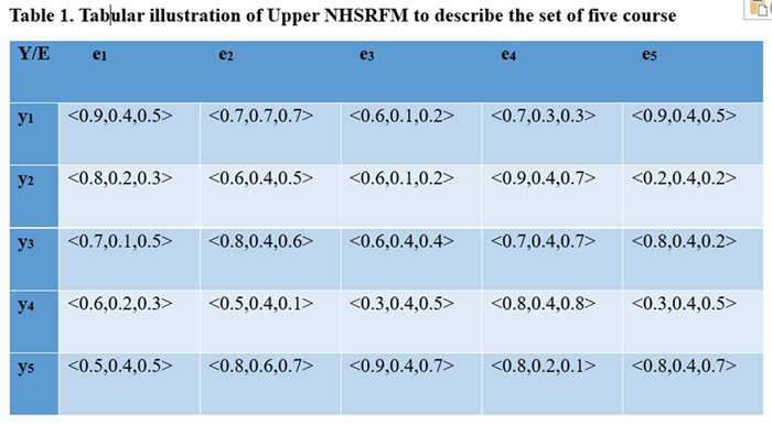
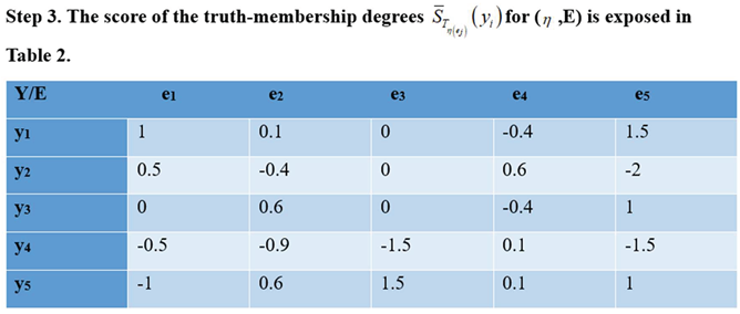
Step 4. The score of the degree of indeterminacy degrees for (,E) is exposed in Table 3.
| Y/E | e1 | e2 | e3 | e4 | e5 | |
| y1 | 0.7 | 1 | -0.9 | -0.2 | 0 | |
| y2 | -0.3 | -0.5 | -0.9 | 0.3 | 0 | |
| y3 | -0.8 | -0.5 | 0.6 | 0.3 | 0 | |
| y4 | -0.3 | -0.5 | 0.6 | 0.3 | 0 | |
| y5 | 0.7 | 0.5 | 0.6 | -0.7 | 0 |

| Y/E | e1 | e2 | e3 | e4 | e5 |
| y1 | 0.4 | 0.9 | -1 | -1.1 | 0.4 |
| y2 | -0.6 | -0.1 | -1 | 0.9 | -1.1 |
| y3 | 0.4 | 0.1 | 0 | 0.9 | -1.1 |
| y4 | -0.6 | -2.1 | 0.5 | 1.4 | 0.4 |
| y5 | 0.4 | 0.9 | 1.5 | -2.1 | 1.4 |

| Y/E | e1 | e2 | e3 | e4 | e5 |
| y1 | 2.1 | 2 | -1.9 | -1.7 | 1.9 |
| y2 | -0.4 | -1 | -1.9 | 1.8 | -3.1 |
| y3 | -0.4 | -1 | 0.6 | 0.8 | -0.1 |
| y4 | -1.4 | -3.5 | -0.4 | 1.8 | -1.1 |
| y5 | -1.3 | 2 | 3.6 | -2.7 | 2.4 |
Step 7: Computation of the Overall Scores
The overall score values v1 = 2.4, v2 = -4.6, v3 = -0.1, v 4 = -4.6, v5 = 4.
obtained for the five engineering courses are calculated as follows:
Step:6 Selection of the Optimal Alternative
The maximum score among all alternatives is determined by v5.
Since v5 has the highest score, the engineering course v5 is identified as the most suitable alternative. Therefore, v5 is selected as the optimal choice for the decision-maker.
12. Conclusion and Future Work
In this study, we have analysed idempotent NHSRFMs and specifically focused on the subclass of idempotent NHSRFMs of T-type. Through the establishment of key properties and theorems, we have demonstrated foundational characteristics that define and distinguish these matrices. The numerical example provided effectively illustrates the application and practical relevance of these theoretical findings, affirming the consistency and utility of the proposed theorems.
Furthermore, the development of a DM algorithm based on NHSRFMs offers a structured and systematic approach for tackling complex DM scenarios. The algorithm’s effectiveness is underscored through an illustrative example, showcasing the potential of NHSRFMs in real-world applications. This work contributes to the field of NHSRFM theory, enhancing its applicability in DM contexts and providing a framework for further research and development in this area.
Future work on idempotent NHSRFMs could involve exploring additional subclasses and extending properties to other neutrosophic structures, such as tensors, to broaden their theoretical foundation. Refining the decision-making algorithm with advanced methods like multi-criteria optimization or machine learning could also improve its applicability in complex scenarios. Applying the algorithm in real-world contexts, such as environmental management and healthcare, would validate its robustness. Additionally, developing software tools for NHSRFMs could make these methods more accessible, supporting further research and practical use in DM applications.
Author Contributions
Conceptualization, M. Rajalakshmi, C. Priyadharshini Infanta, Surapati Pramanik and Florentin Smarandache; Methodology, M. Rajalakshmi, C. Priyadharshini Infanta, Surapati Pramanik and Florentin Smarandache; Software, M. Rajalakshmi, C. Priyadharshini Infanta and Surapati Pramanik; Validation, M. Rajalakshmi, C. Priyadharshini Infanta and Surapati Pramanik; Formal analysis, M. Rajalakshmi, C. Priyadharshini Infanta, Surapati Pramanik and Florentin Smarandache; Investigation, M. Rajalakshmi, C. Priyadharshini Infanta, Surapati Pramanik and Florentin Smarandache; Resources, M. Rajalakshmi, C. Priyadharshini Infanta, Surapati Pramanik and Florentin Smarandache; Data curation, M. Rajalakshmi, C. Priyadharshini Infanta, Surapati Pramanik and Florentin Smarandache; Writing – original draft, M. Rajalakshmi, C. Priyadharshini Infanta, Surapati Pramanik and Florentin Smarandache; Writing – review & editing, M. Rajalakshmi, C. Priyadharshini Infanta and Florentin Smarandache; Visualization, M. Rajalakshmi, C. Priyadharshini Infanta, Surapati Pramanik and Florentin Smarandache; Supervision, M. Rajalakshmi, C. Priyadharshini Infanta, Surapati Pramanik and Florentin Smarandache; Funding acquisition, Florentin Smarandache. All authors have read and agreed to the published version of the manuscript.
Funding
This research received no external funding.
Data Availability Statement
No new data were created or analyzed in this study.
Conflicts of Interest
The authors declare no conflict of interest.
References
- Zadeh, L.A. Fuzzy sets. Inf. Control 1965, 8, 338–353. [Google Scholar] [CrossRef]
- Atanassov, K.T. Intuitionistic fuzzy sets. Fuzzy Sets Syst. 1986, 20, 87–96. [Google Scholar] [CrossRef]
- Jang, L.C.; Kim, W.J.; Kim, T. A note on distances between interval-valued intuitionistic fuzzy sets. Int. J. Fuzzy Log. Intell. Syst. 2011, 11, 8–11. [Google Scholar] [CrossRef]
- Park, J.H.; Kwun, Y.C.; Son, M.J. A generalized intuitionistic fuzzy soft set theoretic approach to decision making problems. Int. J. Fuzzy Log. Intell. Syst. 2011, 11, 71–76. [Google Scholar] [CrossRef]
- Kim, K.H.; Roush, F.W. Generalized fuzzy matrices. Fuzzy Sets Syst. 1980, 4, 293–315. [Google Scholar] [CrossRef]
- Thomason, M.G. Convergence of powers of a fuzzy matrix. J. Math. Anal. Appl. 1977, 57, 476–480. [Google Scholar] [CrossRef]
- Kim, J.B. Idempotents and inverse in fuzzy matrices. Bull. Malays. Math. Sci. Soc. 1983, 6, 57–61. [Google Scholar]
- Mishref, M.A.; Emam, E.G. Transitivity and subinverses in fuzzy matrices. Fuzzy Sets Syst. 1992, 52, 337–343. [Google Scholar] [CrossRef]
- Ragab, M.Z.; Emam, E.G. The determinant and adjoint of a square fuzzy matrix. Inf. Sci. 1995, 84, 209–220. [Google Scholar] [CrossRef]
- Kim, J.B. On fuzzy idempotent matrices of T-type. Inf. Sci. 1994, 80, 311–318. [Google Scholar] [CrossRef]
- Meenakshi, A.R. Fuzzy Matrix: Theory and Applications; MJP Publishers: Chennai, India, 2008. [Google Scholar]
- Pal, M. Intuitionistic fuzzy determinant. V.U.J. Phys. Sci. 2001, 7, 87–93. [Google Scholar]
- Im, Y.B.; Lee, E.P.; Park, S.W. The determinant of square intuitionistic fuzzy matrices. Far East J. Math. Sci. 2001, 3, 789–796. [Google Scholar]
- Pal, M.; Khan, S.K.; Shyamal, A.K. Intuitionistic fuzzy matrices. Notes Intuitionistic Fuzzy Sets 2002, 8, 51–62. [Google Scholar]
- Shyamal, A.K.; Pal, M. Two new operators on fuzzy matrices. J. Appl. Math. Comput. 2004, 15, 91–107. [Google Scholar] [CrossRef]
- Shyamal, A.K.; Pal, M. Distances between intuitionistic fuzzy matrices. V.U.J. Phys. Sci. 2002, 8, 81–91. [Google Scholar]
- Bhowmik, M.; Pal, M. Generalized intuitionistic fuzzy matrices. Far East J. Math. Sci. 2008, 29, 533–554. [Google Scholar]
- Bhowmik, M.; Pal, M. Generalized interval-valued intuitionistic fuzzy sets. J. Fuzzy Math. 2010, 18, 357–371. [Google Scholar]
- Bhowmik, M.; Pal, M. Some results on generalized interval-valued intuitionistic fuzzy sets. Int. J. Fuzzy Syst. 2012, 14, 193–203. [Google Scholar]
- Khan, S.K.; Pal, A. The generalized inverse of intuitionistic fuzzy matrices. J. Phys. Sci. 2007, 11, 62–67. [Google Scholar]
- Adak, A.K.; Bhowmik, M.; Pal, M. Some properties of generalized intuitionistic fuzzy nilpotent matrices over distributive lattice. Fuzzy Inf. Eng. 2012, 4, 371–387. [Google Scholar] [CrossRef]
- Padder, R.A.; Murgadas, P. Max-max operation on intuitionistic fuzzy matrix. Ann. Fuzzy Math. Inform. In press.
- Murugadas, P.; Padder, R.A. Reduction of an intuitionistic fuzzy rectangular matrix. Annamalai Univ. Sci. J. 2015, 49, 15–18. [Google Scholar]
- Pradhan, R.; Pal, M. Convergence of max-arithmetic mean-min-arithmetic mean powers of intuitionistic fuzzy matrices. Int. J. Fuzzy Math. Arch. 2013, 2, 58–69. [Google Scholar]
- Sriram, S.; Murugadas, P. On semiring of intuitionistic fuzzy matrices. Appl. Math. Sci. 2010, 4, 1099–1105. [Google Scholar]
- Sriram, S.; Murugadas, P. Sub-inverses of intuitionistic fuzzy matrices. Acta Cienc. Indica Math. 2011, 37, 41–56. [Google Scholar]
- Lee, H.Y.; Jeong, N.G. Canonical form of a transitive intuitionistic fuzzy matrix. Honam Math. J. 2005, 27, 543–550. [Google Scholar]
- Atanassov, K. Generalized index matrices. C. R. Acad. Bulg. Sci. 1987, 40, 15–18. [Google Scholar]
- Atanassov, K.T. Intuitionistic fuzzy sets. In Proceedings of the Polish Symposium on Interval and Fuzzy Mathematics (VII ITKR's Session), Sofia, Bulgaria, 1983. [Google Scholar]
- Im, Y.B.; Lee, E.P.; Park, S.W. The adjoint of square intuitionistic fuzzy matrices. J. Appl. Math. Comput. 2003, 11, 401–412. [Google Scholar]
- Padder, R.A.; Murugadas, P. On idempotent intuitionistic fuzzy matrices of T-type. Int. J. Fuzzy Log. Intell. Syst. 2016, 16, 181–187. [Google Scholar] [CrossRef]
- Uma, R.; Murugadas, P.; Sriram, S. Determinant theory for fuzzy neutrosophic soft matrices. Prog. Nonlinear Dyn. Chaos 2016, 4, 85–102. [Google Scholar]
- Uma, R.; Sriram, S.; Murugadas, P. Fuzzy neutrosophic soft matrices of Type I and Type II. Fuzzy Inf. Eng. 2021, 13(2), 211–222. [Google Scholar] [CrossRef]
- Smarandache, F. Neutrosophic set, a generalization of the intuitionistic fuzzy set. Int. J. Pure Appl. Math. 2005, 24, 287–297. [Google Scholar]
- Anandhkumar, M.; Harikrishnan, T.; Chithra, S.M.; Kamalakannan, V.; Kanimozhi, B. Partial orderings, characterizations and generalization of k-idempotent neutrosophic fuzzy matrices. Int. J. Neutrosophic Sci. 2024, 23, 286–295. [Google Scholar]
- Anandhkumar, M.; Kamalakannan, V.; Chithra, S.M.; Said, B. Pseudo similarity of neutrosophic fuzzy matrices. Int. J. Neutrosophic Sci. 2023, 20, 191–196. [Google Scholar]
- Raut, P. K.; Rajalakshmi, R.; Saritha, K.; Gayathri Lakshmi, M. A novel bipolar neutrosophic soft topological model for agricultural decision analysis. Int. J. Reason.-Based Intell. Syst. 2026. [Google Scholar] [CrossRef]
- Peng, X.; Dai, J. A bibliometric analysis of neutrosophic set: Two decades review from 1998 to 2017. Artif. Intell. Rev. 2020, 53, 199–255. [Google Scholar] [CrossRef]
- Pramanik, S. Single-valued neutrosophic set: An overview. In Transdisciplinarity; Rezaei, N., Ed.; Integrated Science Series; Springer: Cham, Switzerland, 2022; Vol. 5, pp. 563–608. [Google Scholar] [CrossRef]
Figure 1.
Algorithm of the Decision-Making Using NHSRFM.
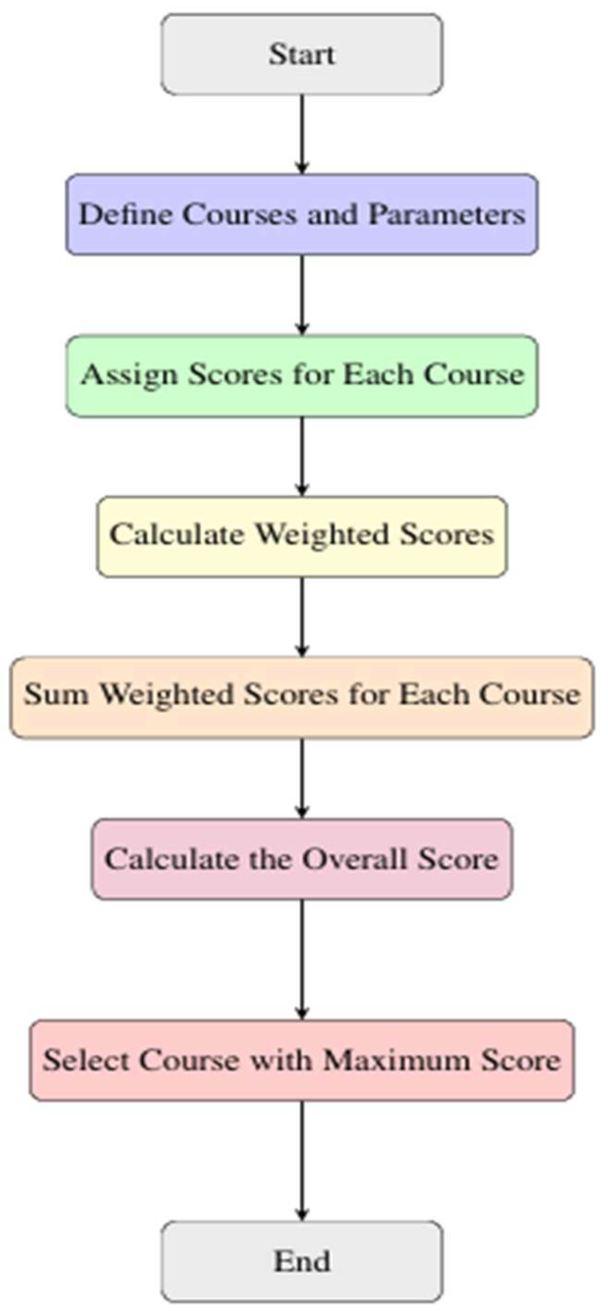
Figure 2.
Algorithm to identify the most suitable course.
Disclaimer/Publisher’s Note: The statements, opinions and data contained in all publications are solely those of the individual author(s) and contributor(s) and not of MDPI and/or the editor(s). MDPI and/or the editor(s) disclaim responsibility for any injury to people or property resulting from any ideas, methods, instructions or products referred to in the content. |
© 2026 by the authors. Licensee MDPI, Basel, Switzerland. This article is an open access article distributed under the terms and conditions of the Creative Commons Attribution (CC BY) license (http://creativecommons.org/licenses/by/4.0/).
Copyright: This open access article is published under a Creative Commons CC BY 4.0 license, which permit the free download, distribution, and reuse, provided that the author and preprint are cited in any reuse.


