

Submitted:
02 June 2026
Posted:
03 June 2026
You are already at the latest version
Abstract
Low-cost air quality sensors can expand PM₂.₅ monitoring networks but require calibration against regulatory-grade monitors to correct systematic bias. Although interest in predictive uncertainty for air quality estimation has increased, uncertainty reliability under spatial sparsity and wildfire-induced distribution shift remains poorly understood. This study develops a transformer-based PM₂.₅ calibration model and evaluates two uncertainty quantification methods, GeoConformal Prediction (GCP) and Monte Carlo Dropout (MCD), using sensor pairs in California and the Northeast United States. The calibration model achieved strong performance at short spatial distances, with test R² values of 0.89 and 0.91 at the 1 km threshold in California and the Northeast, respectively, with accuracy declining as sensor separation increased. GCP generally produced calibration curves closer to the ideal diagonal, while MCD generated tighter prediction intervals under normal conditions. During wildfire events, uncertainty performance depended on sensor separation. At short distances, MCD expanded its uncertainty intervals and captured PM₂.₅ spikes more effectively than GCP (71% vs. 61% coverage). At larger separations, MCD captured only 44% of elevated observations, whereas GCP widened its intervals and achieved 83% coverage. These results demonstrate that uncertainty reliability is strongly influenced by spatial separation and environmental conditions, highlighting the need for uncertainty-aware calibration of low-cost PM₂.₅ sensors.
Keywords:
PM₂.₅
; calibration
; uncertainty quantification
; air quality
; low-cost sensors
; wildfire
; transformers
; Monte Carlo Dropout
; GeoConformal prediction
1. Introduction
Air pollution, exacerbated by climate-driven events like wildfires, poses significant risks to both air quality and human health [1]. Fine particulate matter (PM₂.₅) is of particular concern because it can penetrate deep into the respiratory system and is strongly associated with adverse health outcomes, underscoring the need for accurate monitoring [2]. Regulatory-grade sensors such as those from the United States Environmental Protection Agency (EPA) provide high-quality measurements but are limited in number and spatial coverage. As a result, they often fail to capture localized pollution variability, especially during extreme events [3]. This limitation becomes particularly important during wildfire events, where PM₂.₅ concentrations can vary substantially across space, even within the same region [4]. As a result, there is a growing need for monitoring approaches that can capture localized air quality dynamics beyond the coverage of existing regulatory networks.
Low-cost sensors (LCS) have emerged as a promising supplementary technology for regulatory monitoring networks owing to their affordability, accessibility, and small size, enabling denser spatial coverage [5]. Expanding low-cost sensor networks can help preserve air quality monitoring coverage when individual sensors fail or are destroyed during extreme events [6]. Among the most widely deployed LCS networks, PurpleAir operates tens of thousands of community-based sensors globally, offering near-real-time PM₂.₅ data at high spatiotemporal resolution [7]. While PurpleAir's real-time sensor readings are publicly viewable, bulk and historical data access through their API requires a paid subscription, limiting its utility for large-scale retrospective research [2]. Clarity, another LCS network, provides community-scale PM₂.₅ monitoring with publicly accessible data, making it a viable alternative for research applications [8]. Raw measurements from these LCS require calibration to correct systematic bias relative to regulatory-grade monitors [9]. This calibration is typically performed using statistical or machine learning models that learn relationships between sensor readings, meteorological variables, and reference observations [10]. Once calibrated, these models are used to generate spatial predictions or interpolations of PM₂.₅ concentrations, particularly in areas lacking dense monitoring coverage [11].
Despite improvements in calibration accuracy, most studies evaluate sensor performance using metrics such as mean absolute error (MAE), root mean square error (RMSE), or coefficient of determination (R2). These metrics quantify average error but do not assess prediction reliability or confidence under different conditions [5,12]. This limitation is especially critical during wildfire events, which can introduce substantial distribution shifts in PM₂.₅ concentrations relative to typical training conditions [7]. To address this gap, several model-based uncertainty quantification (UQ) methods, including Bayesian neural networks (BNNs), Monte Carlo Dropout (MCD), and deep ensembles (DE), have been developed to quantify uncertainties by modeling variability in model outputs [13]. These UQ methods remain dependent on model assumptions and the representativeness of the training distribution [14]. Under a wildfire-induced distribution shift, model-derived uncertainty may become miscalibrated, leading to overconfident or unreliable prediction intervals [15]. On the other hand, conformal prediction has emerged as a distribution-free alternative for UQ that constructs prediction intervals from observed residual errors, providing distribution-free coverage guarantees [16,17]. GeoConformal prediction (GCP) extends this framework to spatial settings by weighting calibration errors according to geographic proximity, producing location-dependent prediction intervals with formal coverage guarantees [14].
While interest in predictive uncertainty for air quality estimation has grown, a critical gap remains in the systematic evaluation of the reliability of predictive uncertainty under conditions of spatial sparsity and wildfire-induced distribution shift. This study addresses this gap by systematically evaluating GCP and MCD reliability for low-cost PM₂.₅ sensor calibration across varying sensor separations and wildfire conditions, establishing a reliability-centered framework for UQ. The research objectives are listed below:
- Develop a transformer-based model for PM₂.₅ calibration and quantify uncertainty using GCP and MCD to produce reliable, well-calibrated estimates with uncertainty bounds across two study areas, California (CA) and the Northeast (NE) United States.
- Analyze how calibration performance and UQ reliability vary with increasing spatial distance between collocated sensor pairs (1 km, 5 km, and 10 km thresholds) across both study areas, to understand the spatial limitations of LCS calibration.
- Evaluate and compare the reliability of GCP and MCD under wildfire and non-wildfire conditions, focusing on empirical coverage and interval width to assess how wildfire-induced distribution shift affects each uncertainty method.
The remainder of this paper is organized as follows. Section 2 reviews prior research on UQ for low-cost PM₂.₅ sensor calibration, including performance under wildfire conditions. Section 3 introduces the study area and datasets used in this work. Section 4 presents the calibration modeling framework, experimental design, and evaluation metrics. Section 5 presents the UQ results and reliability analysis, followed by a discussion in Section 6 and conclusions in Section 7.
2. Literature Review
This section reviews the literature relevant to the three core dimensions of this study. Section 2.1 examines recent advances in low-cost PM₂.₅ sensor calibration, including machine-learning and deep-learning methods that form the basis of the calibration framework used in this work. Section 2.2 discusses the challenges of air quality monitoring during wildfire events, in which extreme PM₂.₅ concentrations can degrade both calibration accuracy and uncertainty estimates. Section 2.3 surveys existing UQ methods for LCS calibration, identifying the gap between model-based approaches, such as MCD, and distribution-free alternatives, such as GCP, that this study aims to address.
2.1. Low-Cost Air Quality Sensor Calibration
Recent research on low-cost PM₂.₅ sensor calibration has increasingly emphasized the importance of field calibration under real-world deployment conditions, as raw measurements from LCS often exhibit systematic bias relative to regulatory-grade sensors. One study focusing on field-based calibration demonstrated that accounting for PM₂.₅ levels and temperature can reduce bias and improve agreement with reference monitors [18]. Specifically, LCS are highly sensitive to environmental factors such as temperature, humidity, and pollutant composition, and calibration approaches that do not account for this variability may not generalize well when applied across diverse settings, highlighting the risk of deploying sensors without local calibration [19,20].
Expanding on this, recent work applies machine-learning-based calibration methods to improve agreement between LCS and reference-grade monitors [21]. Multiple studies demonstrate that machine learning calibration can significantly reduce systematic error and improve model performance relative to raw sensor measurements [22,23,24]. Traditional machine learning models such as linear regression, random forest, and gradient boosting, provide strong baseline calibration performance [10,25,26]. More recently, deep learning approaches show superior results, with recurrent neural network (RNN) models such as Long Short-Term Memory (LSTM) capturing temporal dependencies in sensor data and outperforming traditional machine learning approaches for PM₂.₅ calibration [12]. A systematic evaluation of machine learning models for LCS calibration further confirms that LSTM outperforms traditional approaches [2]. Despite these advances, most deep learning calibration studies do not evaluate predictive uncertainty, limiting the ability to assess the reliability of individual estimates, a gap that motivates the formal UQ methods examined in Section 2.3.
2.2. Low-Cost Air Quality Sensing During Wildfires
Wildfires are an increasingly common source of extreme PM₂.₅ exposure, yet regulatory monitoring networks often lack the spatial coverage needed to capture localized smoke impacts [27]. Studies demonstrated that networks of LCS can fill critical spatial gaps, enabling detailed monitoring of rapid PM₂.₅ increases across indoor, outdoor, and personal exposure settings [3]. When appropriate device-specific adjustment factors are applied, LCS achieve mean absolute errors below 10 µg/m3 and substantially improve the accuracy of wildfire smoke detection [28,29]. Integrating LCS with regulatory monitoring networks also improves area-wide concentration estimation during wildfire events and reduces interpolation error by over 20% [30]. These findings support the use of LCS for capturing local PM₂.₅ concentrations during wildfire events, especially in regions lacking coverage from regulatory monitors.
However, wildfire events can introduce a significant dataset shift because PM₂.₅ concentrations and environmental conditions during smoke episodes may differ substantially from those represented in the model training data [7]. Such shifts can reduce the generalizability of calibration models and lead to degraded performance, as distributional differences between training and deployment data are a recognized challenge in geospatial machine learning applications [31]. Furthermore, uncertainty estimates that appear well calibrated under in-distribution conditions may become unreliable under dataset shift [15]. While previous studies have primarily focused on improving calibration accuracy during wildfire events, limited attention has been given to systematically evaluating the reliability of calibrated PM₂.₅ estimates and their associated uncertainty estimates under these conditions.
2.3. Uncertainty in LCS Calibration
In this section, two forms of spatial shift in PM₂.₅ calibration are reviewed: variation in PM₂.₅ characteristics and calibration performance across geographic regions and increasing distance between LCS and reference monitors. Firstly, calibration performance can vary across geographic regions due to differences in aerosol composition, meteorology, emissions, and environmental conditions [32]. These regional differences can reduce model transferability and lead to degraded calibration accuracy when models are applied outside the conditions represented in the training data [33]. To address this, a recent work has advocated for region-specific calibration and validation strategies that account for local aerosol and meteorological conditions [34]. Secondly, fine-scale spatial variability in PM₂.₅ measurements can occur even between nearby sensors, reflecting local pollution sources and heterogeneity in observed concentrations [35]. This spatial heterogeneity results in reduced agreement between low-cost and regulatory PM₂.₅ sensors with increasing distance from reference monitors [36,37]. Zhivkov and Fidanova [38] showed that the calibration uncertainty increases with distance from reference monitors, leading to reduced reliability of measurements at greater distances. However, their quantified uncertainty as a distance-dependent empirical growth rate but does not provide individual prediction-level uncertainty or adapt to changing environmental conditions.
Together, these findings highlight that while LCS calibration has advanced considerably through various approaches, most studies have focused on predictive accuracy and have lacked systematic uncertainty quantification. While our previous work systematically compared model-based UQ methods such as BNNs, MCD, and DE for geospatial air quality monitoring [39], it did not evaluate spatially adaptive, distribution-free UQ methods for calibrated PM₂.₅ estimates. This study addresses these gaps by systematically evaluating both model-based and model-agnostic UQ methods for transformer-based PM₂.₅ calibration. A major contribution of this study is the evaluation of GCP as a spatially adaptive, distribution-free UQ framework that generates geographically informed prediction intervals with formal coverage guarantees. In addition, this study systematically examines how uncertainty reliability varies across increasing collocation distances between low-cost and reference sensors and under wildfire-induced distribution shifts.
3. Study Area and Data
3.1. Study Area
This study focuses on two geographically distinct study areas, California and the Northeast United States. These two regions were selected because they represent contrasting aerosol compositions, regulatory monitoring densities, and wildfire exposure regimes, enabling evaluation of model generalizability across climatically and geographically diverse conditions. Figure 1 and Figure 2 depict the locations of AirNow and Clarity sensors across both study areas. In California, 147 AirNow monitors and 1,022 Clarity sensors were used, concentrated in the Los Angeles and San Francisco metropolitan areas. In the Northeast United States, 157 AirNow monitors and 101 Clarity sensors were used. AirNow monitors provide broad spatial coverage across both study areas, while Clarity sensors offer dense coverage over urban regions, which is critical for capturing localized PM₂.₅ variability and supporting high-resolution calibration during extreme events.
Two wildfire events were used as case studies to evaluate model performance under extreme PM₂.₅ conditions. In California, the Palisades Fire and Eaton Fire ignited on January 7, 2025, becoming among the most destructive wildfires in California history [40]. The Palisades Fire burned approximately 23,448 acres in the Pacific Palisades and Malibu areas, while the Eaton Fire burned approximately 14,021 acres near Altadena and Pasadena, collectively causing severe PM₂.₅ degradation across the Los Angeles basin [41]. In the Northeast United States, the Jennings Creek Wildfire ignited in November 2024 along the border of New York and New Jersey, burning approximately 5,000 acres, prompting health advisories for unhealthy air quality across the region [42]. Together, these wildfire events provide distinct and complementary case studies for evaluating the reliability of UQ methods under wildfire-induced distribution shift across both study areas.
3.2. Data Acquisition
3.2.1. AirNow
Hourly ground-level PM₂.₅ concentrations from 2022–2025 were obtained from the U.S. EPA AirNow network via the AirNow API [43]. AirNow is a national air quality reporting partnership that aggregates monitoring data from federal, state, tribal, and local agencies across the United States [44]. Monitoring agencies submit observations from regulatory-grade air quality monitors to AirNow's centralized system, which provides standardized national reporting and near-real-time quality control. These observations served as reference measurements for sensor calibration and uncertainty evaluation.
3.2.2. Clarity
The Clarity Node-S is a low-cost optical particle counter that measures PM₂.₅ via laser light scattering, with raw measurements recorded at minute-level temporal resolution [45]. For this study, hourly aggregated PM₂.₅ data were downloaded from the OpenAQ measurements API [46] for the period 2022–2025. These data were collocated with AirNow regulatory-grade monitors and used as the primary LCS input to develop and train calibration models.
3.2.3. Meteorological Variables
Hourly meteorological variables, including 2m temperature, 2m relative humidity, 10m wind speed, and pressure, were obtained from the National Oceanic and Atmospheric Administration (NOAA) High-Resolution Rapid Refresh (HRRR) model, a real-time 3-km resolution hourly updated atmospheric model covering the contiguous United States. HRRR data were downloaded from the NOAA archive hosted on Amazon Web Services (AWS) Simple Storage Service (S3) (s3://noaa-hrrr-bdp-pds) using the 2D surface-level fields at a 3-km spatial resolution. Relative humidity and temperature are the primary meteorological drivers of the bias in the LCS, as high humidity causes hygroscopic particle growth that inflates optical scattering signals, while temperature affects sensor electronics and particle composition, both of which systematically distort PM₂.₅ readings [47,48]. These variables were extracted at the collocated sensor locations and temporally matched to hourly PM₂.₅ observations.
3.2.4. Ancillary Variables
Land use and land cover (LULC) data were obtained from the National Land Cover Database (NLCD), produced by the United States Geological Survey (USGS) at 30m spatial resolution [49]. Federal Information Processing Standards (FIPS) codes were used to identify county-level administrative boundaries for each sensor location [50]. Geographic coordinates, including latitude and longitude, were included to enable spatial matching between collocated sensor pairs. Temporal categorical variables such as hour of day, day, month, season, day of year (DoY), day of week (DoW), and week of year (WoY) were derived from each observation's timestamp to capture diurnal, weekly, and seasonal cycles in PM₂.₅ concentrations.
4. Methodology
Figure 3 illustrates the overall research workflow, beginning with data acquisition from OpenAQ LCS and EPA regulatory monitors, followed by data collocation, preprocessing, and train-test splitting. The processed data are used to train a Transformer-based calibration model, which produces calibrated PM₂.₅ estimates. These calibrated PM₂.₅ estimates are then used to quantify uncertainty and assess reliability under wildfire events.
4.1. Data Collocation
Raw PM₂.₅ measurements from Clarity sensors were first subjected to outlier removal using a rolling standard deviation filter. Records with a rolling standard deviation of zero were excluded to remove inactive or non-reporting sensor readings. Following outlier removal, Clarity sensors were spatiotemporally collocated with the nearest AirNow regulatory-grade monitors at distance thresholds of 1 km, 5 km, and 10 km, retaining only sensor pairs with a Pearson correlation coefficient of 0.4 or higher to ensure a minimum level of measurement agreement before calibration.
Table 1 summarizes the collocated sensor pair statistics across both study areas. In the Northeast, the number of collocated pairs increased from 4 at 1 km to 19 at 10 km, with mean correlations ranging from 0.87 at 1 km to 0.81 at 10 km. In California, pairs increased from 11 at 1 km to 27 at 10 km, with mean correlations ranging from 0.80 at 1 km to 0.77 at 10 km. Across both study areas, the correlation declined as sensor separation distance increased. In contrast, the number of available pairs increased, reflecting a trade-off between spatial proximity and the availability of collocated sensor pairs for model training.
4.2. Data Preprocessing
This study applied several preprocessing steps to the collocated dataset before training, including gap-filling for missing values, data splitting, feature scaling, and sequence construction. Missing PM₂.₅ values were imputed using an XGBoost-based model trained separately for each region, achieving R² of 0.88 and RMSE of 2.81 µg/m³ for California, and R² of 0.89 and RMSE of 1.43 µg/m³ for the Northeast [51]. FIPS codes and LULC were incorporated as categorical variables to capture county-level administrative context and surface environment characteristics at each sensor location. The collocated dataset was then partitioned using a time-based split with 70% of the data used for training, 10% for validation, and 20% for testing, ensuring that all sets are temporally non-overlapping, preventing data leakage, and reflecting real-world deployment conditions. Input features were subsequently normalized using a standard scaler to ensure consistent scaling across continuous variables. Finally, the data were organized into sequential input windows of 23 preceding hourly observations, with each sequence used to calibrate the current-hour PM₂.₅ measurement. The sequence length of 23 was selected to capture near-diurnal temporal dependencies while maintaining computational efficiency [52].
4.3. Transformer Model Architecture
The proposed calibration model is based on a transformer architecture, which was introduced by [53]. Transformers capture long-range temporal dependencies through self-attention mechanisms while processing entire input sequences in parallel. This makes them well-suited for PM₂.₅ calibration, where capturing temporal patterns across the input window is essential [54]. The proposed model takes continuous and categorical spatio-temporal variables as input, producing a multi-step sequence of calibrated PM₂.₅ estimates. A schematic overview of the model architecture is presented in Figure 4.
4.3.1. Inputs/Embedding
Categorical temporal variables, including hour, day, season, month, DoY, DoW, and WoY, as well as location indicators, are represented using learnable embedding layers that map each category to a continuous vector representation. These embeddings allow the model to capture relationships among discrete temporal and spatial features. The resulting categorical embeddings are concatenated with continuous input features, including temperature, pressure, and humidity, to form the complete input sequence. This combined representation allows the model to learn from both discrete and continuous spatiotemporal information jointly.
4.3.2. Positional Encoding
Learnable positional embeddings are added to the projected sequence representation to preserve temporal relationships within the input data. Since the Transformer architecture does not inherently encode sequence order, positional information must be explicitly incorporated into the input representations [53]. These embeddings provide information about the position of each element in the sequence, enabling the model to distinguish between different temporal arrangements. This allows the self-attention mechanism to account for sequence order, enabling the model to capture temporal structure during both training and inference.
4.3.3. Encoder
The encoder consists of a stack of identical encoder layers. Each encoder layer includes multi-head self-attention followed by a feed-forward network. Residual connections and layer normalization are applied around both sublayers [53].
In the self-attention sub-layer, the input representation is linearly projected into query (Q), key (K), and value (V) matrices. The relationships between different positions in the sequence are computed using scaled dot-product attention, defined as Equation (1)
where Q, K, and V denote the query, key, and value matrices, and dk represents the dimensionality of the key vectors. The resulting attention outputs from multiple heads are concatenated and passed to the feed-forward network within the encoder layer. The encoder produces a transformed sequence representation that serves as memory for the decoder.
4.3.4. Decoder
The decoder also consists of stacked decoder layers. Each decoder layer includes self-attention, encoder-decoder attention, and a feed-forward network, with residual connections and layer normalization applied after each component. The decoder processes the encoded sequence representation to generate the final calibrated PM₂.₅ estimates.
4.4. Model Training
The decoder output is passed through a hidden linear projection layer to produce the predicted mean (μ) and variance (σ²) of PM₂.₅ concentrations. Model parameters are optimized using a hybrid loss function that combines Gaussian negative log-likelihood (NLL) and a weighted Huber loss [55]. The NLL term enables the model to capture aleatoric uncertainty by penalizing errors relative to the predicted variance. At the same time, the weighted Huber loss improves robustness to extreme PM₂.₅ values by reducing the disproportionate influence of large errors. The combined loss function, defined in Equation (2), balances uncertainty calibration with robustness to high PM₂.₅ outliers
The Gaussian Negative Log-Likelihood loss is defined as Equation (3):
where and are the predicted mean and variance for the sample , and balances the two loss components.
4.5. Hyperparameters Optimization
Hyperparameter optimization was performed using random search over a predefined configuration space [56]. The search space included embedding dimensions, the number of attention heads, the number of layers, the feed-forward dimension, the dropout rate, the learning rate, and the batch size. Each configuration was trained with early stopping based on validation R², and the best-performing configuration was selected for final evaluation. The number of attention heads (8), number of layers (5), feed-forward dimension (1024), and optimizer (AdamW) remained consistent across all configurations, while the embedding dimension, batch size, dropout rate, and number of epochs varied across regions and distance thresholds, with the final configurations reported in Table 2.
4.6. Uncertainty Quantification
In this study, two complementary UQ methods are considered: MCD, a model-based method grounded in approximate Bayesian inference, and GCP, a distribution-free framework that provides statistically valid prediction intervals.
MCD, introduced by Gal and Ghahramani [57] provides an efficient framework for estimating predictive uncertainty in deep neural networks by interpreting dropout as a Bayesian approximation to a probabilistic deep Gaussian process. Under this framework, multiple stochastic forward passes are performed during inference with dropout active, producing a distribution of predictions from which the predictive mean and variance are derived. In this study, MCD is extended to jointly capture both epistemic and aleatoric uncertainties by predicting the mean and variance of the target distribution, with the training objective modified to a hybrid NLL loss to enable learning of input-dependent uncertainty. Equation (4) defines the total predictive uncertainty as the sum of epistemic uncertainty and aleatoric uncertainty.
where and denote the predicted mean and variance obtained from the -th stochastic forward pass with dropout enabled, quantifies epistemic uncertainty across all stochastic predictions, and is the total number of stochastic forward passes, set to 30 in this study.
GCP is a model-agnostic UQ framework that extends conformal prediction to spatial prediction tasks [14]. Conformal prediction constructs prediction intervals from a calibration dataset by computing nonconformity scores, typically defined as residuals, and generates intervals with valid marginal coverage under minimal distributional assumptions [16]. The GCP incorporates geographic weighting to account for spatial heterogeneity and covariate shift through a Gaussian distance-decay kernel. It assigns greater weight to nearby calibration points and lower weight to distant ones, where the weight assigned to each calibration point is defined in Equation (5):
where is the location of the calibration point , is the test location, and is the bandwidth parameter controlling the rate of distance decay. The neighborhood included all calibration points without a fixed spatial threshold, and the bandwidth parameter was held constant across all test locations, yielding locally adaptive prediction intervals that reflect spatial heterogeneity.
4.7. Evaluation Metrics
To comprehensively evaluate both calibration performance and uncertainty reliability, this study employs a combination of standard regression metrics and uncertainty-specific metrics. While traditional metrics assess how well the calibration model matches observed PM₂.₅ concentrations, UQ metrics evaluate the reliability of the uncertainty intervals.
4.7.1. Calibration Accuracy Metrics
Standard regression metrics, including R², MAE, MSE, and RMSE, were used to evaluate calibration accuracy, as defined in [39].
4.7.2. Uncertainty Quantification Metrics
Expected Calibration Error (ECE) was used to quantify the difference between predicted confidence and observed coverage, as defined in [39]. Additionally, Prediction Interval Coverage Probability (PICP) and Prediction Interval Width (PIW) were used to evaluate the uncertainty intervals, as defined in Equations (6) and (7), respectively.
Where li and ui denote the lower and upper bounds of the prediction interval for observation i.
where the indicator function equals 1 if the observed value lies within the interval and 0 otherwise.
5. Results
5.1. Statistical Analysis
Exploratory statistical analysis was conducted on PM₂.₅ concentrations from both AirNow and Clarity sensors across two study areas. Boxplots of PM₂.₅ concentrations were used to summarize the central tendency and variability of the data from both sensor types across three distance thresholds (1 km, 5 km, and 10 km), as shown in Figure 5 and Figure 6. In California (Figure 5) the two datasets show similar central tendencies, with median values of 5.1 µg/m³ for AirNow and 4.77 µg/m³ for Clarity. The interquartile ranges are comparable, spanning 3.1-8.2 µg/m³ for AirNow and 2.89-8.07 µg/m³ for Clarity. Despite these similarities, AirNow shows greater variability, with a standard deviation of 6.05 µg/m³ compared to 4.78 µg/m³ for Clarity. AirNow reaches a maximum of 401.1 µg/m³, while Clarity values reach a maximum of 320 µg/m³. The timing of these extreme observations aligns with the 2025 Palisades and Eaton Fires, indicating that these outliers correspond to real pollution events rather than measurement noise.
In the Northeast United States (Figure 6) both sensor types again show comparable central tendencies, though at lower concentrations than in California. AirNow reaches a maximum of 150 µg/m³, while Clarity reaches a maximum of 102 µg/m³, with extreme observations corresponding to smoke transport from Canadian wildfires [58].
To further examine the distributional characteristics, histograms of PM₂.₅ concentrations were analyzed for both AirNow and Clarity sensors across the two study areas, as shown in Figure 7 and Figure 8. In California (Figure 7), both AirNow and Clarity exhibit a strongly right-skewed distribution, with the majority of observations concentrated between approximately 3 and 8 µg/m³. Both sensors report similar typical PM₂.₅ values, with long upper tails corresponding to infrequent but extreme pollution events associated with the 2025 Palisades and Eaton Fires. In the Northeast United States (Figure 8), a similar right-skewed distribution is observed. However, extreme values are notably lower than in California, with upper-tail observations corresponding to smoke transport from Canadian wildfires.
5.2. Model Performance
5.2.1. California
Table 3 presents the model performance metrics across three spatial distance thresholds for California. The model demonstrates strong calibration performance at shorter distances, with test R² values of 0.89, 0.88, and 0.84 at the 1 km, 5 km, and 10 km thresholds, respectively, indicating a gradual decline in accuracy with increasing spatial separation. This decline suggests that increasing spatial separation introduces greater variability and reduces the model's ability to capture localized PM₂.₅ patterns. The gap between training and test performance remains relatively small at shorter distances, indicating limited overfitting when sensors are closely collocated. At larger distances, the increase in error metrics and bias (to 0.2606 µg/m³ at 10 km) suggests reduced generalization and greater difficulty in modeling spatial heterogeneity. These results confirm that calibration accuracy is sensitive to spatial distance, with closer sensor pairs yielding more reliable and consistent predictions.
Figure 9 compares uncalibrated and calibrated PM₂.₅ predictions against reference AirNow observations. The uncalibrated model (Figure 9a) shows substantial dispersion relative to the 1:1 line, with an R² of 0.601, an RMSE of 5.42 µg/m³, and a positive bias of 0.55 µg/m³, indicating systematic overestimation. In contrast, the calibrated model (Figure 9b) exhibits a much tighter alignment with the 1:1 line, with R² improving to 0.893 and RMSE reducing to 2.81 µg/m³. Notably, calibration also substantially reduces the bias from 0.55 to 0.12 µg/m³, demonstrating the model's effectiveness in correcting systematic overestimation of PM₂.₅ concentrations.
5.2.2. Northeast
Table 4 presents the model performance metrics for the Northeast United States across three spatial distance thresholds. Model performance remains strong across all distance thresholds, with only modest increases in error as spatial separation increases. At the 1 km threshold, the model achieves a test R² of 0.91 and RMSE of 1.38 µg/m³, indicating accurate calibration under closely collocated sensor conditions. Compared to California, error metrics in the Northeast are substantially lower across all thresholds, suggesting more consistent and homogeneous PM₂.₅ conditions in this region [59]. As spatial distance increases, performance declines modestly, with test R² decreasing from 0.91 at 1 km to 0.88 at 10 km and RMSE increasing from 1.38 to 1.63 µg/m³. The gap between training and test performance remains small across all distance thresholds, suggesting minimal overfitting and strong generalization. Bias values are consistently negative across all thresholds (ranging from -0.1245 to -0.3200 µg/m³), indicating a systematic tendency for the model to slightly underestimate PM₂.₅ concentrations, though the magnitude remains small.
Figure 10 compares uncalibrated and calibrated predictions against reference observations. The uncalibrated model (Figure 10a) shows substantial dispersion from the 1:1 line, with relatively low explanatory power (R² = 0.402) and higher error (RMSE = 3.60 µg/m³). In contrast, the calibrated model (Figure 10b) demonstrates a significant improvement, with R² increasing to 0.913 and RMSE decreasing to 1.37 µg/m³. Additionally, the reduction in bias from -0.98 µg/m³ to -0.12 µg/m³ highlights the calibration model's effectiveness in correcting systematic underestimation. Overall, these results demonstrate that calibration substantially improves both accuracy and reliability in the Northeast region, with stronger performance compared to California, particularly at larger spatial distances. This is likely because the Northeast has lower PM₂.₅ concentrations with less spatial variability, which reduces prediction difficulty [59], whereas California's complex terrain and episodic wildfire smoke introduce greater concentration heterogeneity that challenges model generalization [60].
5.3. Comparison of MCD and GCP
To further quantify the reliability and practical usefulness of the uncertainty estimates, calibration metrics including PICP, PIW, and ECE were evaluated across multiple confidence levels.
5.3.1. California
Table 5 presents calibration and uncertainty-interval metrics, such as PICP, PIW, and ECE, for MCD and GCP approaches across confidence levels at the 1 km distance threshold in California. The MCD approach demonstrates strong calibration performance, with observed PICP values closely matching the nominal confidence levels. At lower confidence levels, the model exhibits slight underconfidence, with observed PICP values exceeding the nominal levels (e.g., at the 50% confidence level, the observed PICP is 0.55 compared to the ideal of 0.50). At higher confidence levels, however, the trend reverses, with mild undercoverage observed (e.g., at the 99% confidence level, the observed PICP is 0.97 compared to the ideal of 0.99). The relatively low ECE value of 0.02 further confirms that the model is well-calibrated. The prediction intervals widen as expected with increasing confidence levels, with PIW values ranging from 2.37 µg/m³ at the 50% level to 9.12 µg/m³ at the 99% level, reflecting the model's ability to scale uncertainty with confidence appropriately.
The GCP uncertainty approach was evaluated using the same uncertainty metrics to assess its calibration performance. GCP produces values that are generally close to the nominal confidence levels but exhibits consistent undercoverage across all levels. For example, at the 80% and 90% confidence levels, observed PICP values of 0.76 and 0.86 indicate mild undercoverage. The ECE of 0.03 suggests good overall calibration, though slightly worse than MCD. In terms of prediction interval width, GCP produces narrower intervals at lower confidence levels (e.g., 1.67 µg/m³ at 50% vs 2.37 µg/m³ for MCD) but wider intervals at the 99% confidence level (12.90 µg/m³ vs 9.12 µg/m³), suggesting that GCP expands its intervals more aggressively at higher confidence levels to compensate for undercoverage.
The calibration curves for MCD and GCP at the 1 km distance threshold in California are presented in Figure 11. The MCD calibration curve lies predominantly above the ideal diagonal, indicating slight overcoverage at lower confidence levels where the observed PICP values exceed nominal targets. In contrast, the GCP calibration curve consistently falls below the diagonal across the full confidence range, reflecting systematic undercoverage. Notably, while MCD achieves a lower ECE (0.02 vs 0.03), its miscalibration area (0.03) is higher than that of GCP (0.02), suggesting that GCP's curve adheres more closely to the ideal diagonal across the full confidence range despite its slightly higher point-level deviation.
5.3.2. Northeast
Table 6 presents the PICP, PIW, and ECE metrics for MCD and GCP approaches at the 1 km distance threshold in the Northeast. The MCD approach demonstrates good calibration performance, with observed PICP values generally aligning with nominal confidence levels. However, at the 50% confidence level, notable overcoverage is observed (observed PICP of 0.67 vs. ideal of 0.50), while higher confidence levels remain well calibrated (e.g., 90%: 0.91, 99%: 0.97). The ECE of 0.06 is higher than the value observed in California (0.02), indicating a slightly weaker overall calibration in the Northeast. PIW values are consistently lower than in California, ranging from 1.23 µg/m³ at 50% to 4.74 µg/m³ at 99%, suggesting tighter prediction intervals in this region.
The GCP approach in the Northeast shows consistent undercoverage across all confidence levels, with observed PICP values falling short of the nominal levels. Undercoverage is most pronounced at lower confidence levels, with observed PICP values of 0.47, 0.71, and 0.82 at the 50%, 80%, and 90% confidence levels, respectively. The ECE of 0.06 matches that of MCD and is higher than that observed in California, indicating weaker uncertainty calibration in the Northeast. GCP produces notably narrower prediction intervals compared to MCD across all confidence levels (e.g., 0.66 µg/m³ vs. 1.23 µg/m³ at 50%), except for the 99% confidence level (6.01 µg/m³ vs. 4.74 µg/m³), suggesting that GCP expands its intervals more aggressively at higher confidence levels to mitigate its systematic undercoverage.
The calibration curves for MCD and GCP at the 1 km distance threshold in the Northeast are presented in Figure 12. The MCD calibration curve (Figure 12a) lies above the ideal diagonal across much of the confidence range, indicating overcoverage and a higher miscalibration area of 0.08. In contrast, the GCP calibration curve (Figure 12b) falls below the diagonal, indicating systematic undercoverage, but exhibits a lower miscalibration area of 0.03 and remains closer to the ideal diagonal overall. The largest deviations for GCP occur at mid-to-high confidence levels, particularly around the 80% and 90% confidence bounds.
5.4. UQ During Wildfire vs Normal Days
5.4.1. Wildfire Days
Figure 13a–c presents the calibration results for a California wildfire event at 29.40 m sensor separation, characterized by a PM₂.₅ spike exceeding 350 µg/m³. The MCD uncertainty band expands substantially during the peak, achieving 71% coverage of the ground-truth observations during the event (Table 7). In contrast, the GCP interval remains comparatively narrow during the event, resulting in lower coverage.
Figure 13d–f presents the corresponding results for a Northeast wildfire event at 6,798.84 m sensor separation, with PM₂.₅ concentrations reaching approximately 60 µg/m³. In this case, the MCD uncertainty band remains relatively narrow, achieving only 44% coverage of ground-truth observations during the event (Table 7). Conversely, GCP expands its prediction intervals during the event, achieving 83% coverage (Table 7). These results demonstrate that the relative performance of MCD and GCP varies with the spatial and environmental characteristics of wildfire events.
5.4.2. Normal Days
Figure 14 presents the time-series calibration of Clarity PM₂.₅ against AirNow ground truth under normal (non-wildfire) conditions in California (a–c) at 2.92 m and the Northeast (d–f) at 83.69 m spatial separation. Under normal conditions, both methods demonstrate strong calibration performance, with calibrated predictions closely tracking the ground truth across both regions. In California (Figure 14b), the MCD uncertainty band is narrow and efficient, capturing 81% of ground truth observations, while the GCP interval in Figure 14c is consistently wider throughout the time series, capturing 96% of observations.
In the Northeast (Figure 14e), MCD similarly produces narrow, efficient intervals with 73% coverage, while GCP in Figure 14f maintains wider intervals throughout, achieving 92% coverage. The wider GCP intervals reflect its residual-based calibration framework, which prioritizes coverage reliability over interval sharpness [61]. In contrast, MCD estimates uncertainty through stochastic forward passes, producing intervals that more closely follow local prediction variability. Overall, both methods track the ground truth well under normal conditions, with GCP providing higher coverage at the cost of wider intervals and MCD offering more efficient but less conservative uncertainty estimates.
5.5. Spatial Uncertainty
Figure 15 illustrates the spatial distribution of GCP-derived geospatial uncertainty across California at the 1 km distance threshold. The uncertainty varies considerably across sensor locations, ranging from approximately 1 to 6 µg/m³, reflecting the spatially adaptive nature of the GCP framework. Sensors located in the San Francisco Bay Area and along the central coastal region exhibit lower uncertainty values (1–2 µg/m³), suggesting that the model performs more consistently in these areas, likely due to higher sensor density and more homogeneous PM₂.₅ conditions. In contrast, the sensor in the southern coastal region near San Diego exhibits the highest uncertainty (approximately 6 µg/m³), indicating greater prediction variability, which may be attributed to sparse calibration data in the surrounding area or distinct local PM₂.₅ dynamics [62].
6. Discussion
6.1. Comparison of Uncertainty Performance
GCP generally exhibited calibration curves that remained closer to the ideal diagonal than MCD, indicating more consistent calibration across confidence levels [14]. The contrasting overcoverage of MCD and undercoverage of GCP suggest that the two methods characterize predictive uncertainty differently [14,57]. Regional differences indicate that uncertainty calibration is influenced by local spatial characteristics, with both methods exhibiting weaker calibration performance in the Northeast than in California [63]. The Northeast results show that similar ECE values do not necessarily correspond to similar calibration performance. Miscalibration area and calibration curves provided additional insight into uncertainty reliability beyond that captured by ECE alone. These findings emphasize the importance of evaluating uncertainty calibration using multiple complementary metrics rather than relying on a single performance measure.
The event-based analysis revealed important differences in the behavior of MCD and GCP under wildfire and normal conditions. MCD and GCP exhibited a trade-off between interval efficiency and coverage reliability across the evaluated scenarios. Neither method consistently outperformed the other across all wildfire events, with MCD achieving higher coverage during the California wildfire event and GCP achieving substantially higher coverage during the Northeast wildfire event. These differences suggest that the relative performance of UQ methods depends strongly on the spatial and environmental characteristics of the event. The contrasting behavior of the two methods may reflect their different interval construction mechanisms, with MCD deriving uncertainty from model-estimated variance and GCP calibrating interval width using local residual information [14,57]. Under normal conditions, GCP consistently achieved higher coverage through wider prediction intervals, whereas MCD produced narrower and more efficient intervals. Collectively, these findings indicate that method selection should balance interval efficiency and coverage reliability according to the expected degree of spatial separation and distribution shift.
6.2. Comparison with Existing Studies
Table 8 compares this study with recent LCS calibration studies in terms of study area, sensor type, model, performance metrics, wildfire evaluation, and UQ. Compared to existing studies, this study achieved competitive baseline performance (R2=0.89 in California and 0.91 in the NE), comparable to high-performing urban calibration models [12,64] and outperforming tree-based spatial approaches [38,65]. Previous calibration studies, such as Park, Yoo, Park and Lee [12] primarily evaluated calibration performance under standard environmental conditions and did not explicitly assess model reliability during wildfire-driven distribution shifts. Similarly, Delp and Singer [29] addressed wildfire smoke impacts using fixed empirical scaling relationships rather than adaptive deep learning calibration. Furthermore, this study addresses an important gap in the PM₂.₅ calibration literature related to predictive reliability. Previous calibration studies either lacked formal UQ entirely or limited uncertainty analysis to descriptive post-hoc variability assessments [65] or distance-dependent error analyses [38]. In contrast, this study introduces a comparative evaluation of model-based and model-agnostic uncertainty quantification frameworks for low-cost PM₂.₅ sensor calibration. Another major contribution of this work is the systematic evaluation of uncertainty reliability under both normal and extreme pollution conditions, extending calibration assessment beyond predictive accuracy alone. Practically, these prediction intervals can help air quality agencies determine when LCS PM₂.₅ estimates are reliable or uncertain, improving confidence in exposure assessment, wildfire smoke monitoring, and public health decision-making during extreme pollution events.
6.3 Future Directions
Several extensions of this work could further improve calibration robustness and broaden its applicability. Future work should examine the operational deployment of calibrated LCS, where the trustworthiness and reliability of their uncertainty estimates are critical for air-quality decision-making [66]. Such deployment would help translate calibrated estimates into actionable exposure information, extending dependable PM₂.₅ monitoring to underserved communities and supporting timely health advisories during extreme pollution episodes [67]. In this context, method selection should balance interval efficiency against coverage reliability, prioritizing coverage where missed exposures carry the greatest risk [68]. Second, data augmentation strategies, such as generating synthetic sensor observations for under-represented pollution regimes, could improve model robustness and reduce predictive uncertainty during extreme events like wildfires [69]. Targeted augmentation of high-PM₂.₅ episodes is particularly promising given the upper-tail underestimation observed in the wildfire-period results. Third, calibrated LCS could function as a high-resolution observational layer within digital twin systems, densifying the spatial coverage of sparse regulatory networks [70]. Through near-real-time data assimilation, these observations could continuously update the digital twin state, enabling scenario-based forecasting and adaptive air-quality decision-making [71]. Together, these directions point toward a next generation of uncertainty-aware, spatiotemporally adaptive calibration frameworks that can deliver trustworthy PM₂.₅ estimates across diverse environmental conditions.
7. Conclusion
This study presented a systematic evaluation of UQ methods for PM₂.₅ calibration using LCS data, with a focus on reliability under spatial variability and wildfire-induced distribution shift. A transformer-based calibration model was combined with two complementary UQ methods, MCD and GCP, to assess predictive reliability across California and the Northeast United States. The calibration model achieved strong performance at short spatial distances, with test R² values of 0.89 and 0.91 at the 1 km threshold in California and the Northeast, respectively, and accuracy generally decreasing as sensor separation increases, highlighting the sensitivity of calibration to spatial heterogeneity. Both approaches produced reliable uncertainty estimates but differed in how uncertainty is represented based on spatial and temporal constraints. In terms of reliability, GCP generally exhibited calibration curves that more closely followed the ideal diagonal than MCD across the study regions. In practice, MCD provides narrow, efficient intervals under normal conditions and scales effectively during highly localized pollution anomalies. At larger spatial separations, GCP generally achieved higher coverage through wider prediction intervals. These findings demonstrate that uncertainty behavior is highly context-dependent and that event-specific analyses reveal patterns that may not be apparent from aggregate performance metrics alone. To conclude, this study emphasizes the importance of incorporating UQ into air quality workflows to ensure model trustworthiness and reliability under extreme conditions where accurate predictive confidence is essential. Future work should explore data augmentation strategies for high PM₂.₅ events, adaptive calibration approaches for GCP, and hybrid frameworks that combine the complementary strengths of model-based and model-agnostic uncertainty methods.
Author Contributions
Conceptualization, A.S.M., K.S., J.R., G.C., and C.Y.; methodology, A.S.M. and K.S.; software, A.S.M.; validation, A.S.M. and K.S.; formal analysis, A.S.M. and K.S.; investigation, A.S.M. and K.S.; resources, A.S.M.; data curation, S.S.; writing—original draft preparation, A.S.M. and K.S.; writing—review and editing, A.S.M.; visualization, A.S.M. and K.S.; supervision, C.Y.; project administration, C.Y.; funding acquisition, C.Y., G.C., M.P. All authors have read and agreed to the published version of the manuscript.
Funding
This research was funded by NASA AIST and NSF IUCRC, SAI programs.
Data Availability Statement
The low-cost sensor data used in this study were obtained from the OpenAQ platform (https://openaq.org). Reference-grade PM₂.₅ measurements were obtained from the U.S. EPA AirNow network via the AirNow API (https://docs.airnowapi.org/).
Acknowledgments
During the preparation of this manuscript/study, the author(s) used OpenAI ChatGPT 5.5 for the purpose of language checking. The authors have reviewed and edited the output and take full responsibility for the content of this publication.
Conflicts of Interest
The authors declare no conflicts of interest.
Abbreviations
The following abbreviations are used in this manuscript:
| PM₂.₅ | Fine Particulate Matter (≤2.5 micrometers) |
| EPA | Environmental Protection Agency |
| LCS | Low-Cost Sensors |
| UQ | Uncertainty Quantification |
| BNNs | Bayesian Neural Networks |
| MCD | Monte Carlo Dropout |
| DE | Deep Ensembles |
| GCP | GeoConformal Prediction |
| MAE | Mean Absolute Error |
| RMSE | Root Mean Square Error |
| R² | Coefficient of Determination |
| MSE | Mean Square Error |
| NE | Northeast (United States) |
| CA | California |
| RNN | Recurrent Neural Network |
| LSTM | Long Short-Term Memory |
| LULC | Land Use and Land Cover |
| NLCD | National Land Cover Database |
| USGS | United States Geological Survey |
| FIPS | Federal Information Processing Standards |
| DoY | Day of Year |
| DoW | Day of Week |
| WoY | Week of Year |
| NOAA | National Oceanic and Atmospheric Administration |
| HRRR | High-Resolution Rapid Refresh |
| AWS | Amazon Web Services |
| S3 | Simple Storage Service |
| API | Application Programming Interface |
| NLL | Negative Log-Likelihood |
| ECE | Expected Calibration Error |
| PICP | Prediction Interval Coverage Probability |
| PIW | Prediction Interval Width |
| GNN | Graph Neural Network |
References
- Reid, C.E.; Brauer, M.; Johnston, F.H.; Jerrett, M.; Balmes, J.R.; Elliott, C.T. Critical Review of Health Impacts of Wildfire Smoke Exposure. Env. Health Perspect. 2016, 124, 1334–1343. [Google Scholar] [CrossRef]
- Smith, S.; Trefonides, T.; Srirenganathan Malarvizhi, A.; LaGarde, S.; Liu, J.; Jia, X.; Wang, Z.; Cain, J.; Huang, T.; Pourhomayoun, M.; et al. A Systematic Study of Popular Software Packages and AI/ML Models for Calibrating In Situ Air Quality Data: An Example with Purple Air Sensors. Sensors 2025, Vol. 25 2025, 25. [Google Scholar] [CrossRef]
- He, J.; Huang, C.H.; Yuan, N.; Austin, E.; Seto, E.; Novosselov, I. Network of low-cost air quality sensors for monitoring indoor, outdoor, and personal PM2.5 exposure in Seattle during the 2020 wildfire season. Atmos. Environ. 2022, 285, 119244–119244. [Google Scholar] [CrossRef]
- Kramer, A.L.; Liu, J.; Li, L.; Connolly, R.; Barbato, M.; Zhu, Y. Environmental justice analysis of wildfire-related PM2.5 exposure using low-cost sensors in California. Sci. Total Environ. 2023, 856, 159218–159218. [Google Scholar] [CrossRef]
- Concas, F.; Mineraud, J.; Lagerspetz, E.; Varjonen, S.; Liu, X.; Puolamäki, K.; Nurmi, P.; Tarkoma, S. Low-Cost Outdoor Air Quality Monitoring and Sensor Calibration. ACM Trans. Sens. Netw. 2021, 17. [Google Scholar] [CrossRef]
- Chu, H.-J.; Ali, M.Z.; He, Y.-C. Spatial calibration and PM2.5 mapping of low-cost air quality sensors. Sci. Rep. 2020, 10, 22079. [Google Scholar] [CrossRef]
- Barkjohn, K.K.; Holder, A.L.; Frederick, S.G.; Clements, A.L. Correction and Accuracy of PurpleAir PM2.5 Measurements for Extreme Wildfire Smoke. Sensors 2022, 22, 9669. [Google Scholar] [CrossRef]
- Raheja, G.; Nimo, J.; Appoh, E.K.E.; Essien, B.; Sunu, M.; Nyante, J.; Amegah, M.; Quansah, R.; Arku, R.E.; Penn, S.L.; et al. Low-Cost Sensor Performance Intercomparison, Correction Factor Development, and 2+ Years of Ambient PM2.5 Monitoring in Accra, Ghana. Environ. Sci. Technol. 2023, 57, 10708–10720. [Google Scholar] [CrossRef]
- Bi, J.; Wildani, A.; Chang, H.H.; Liu, Y. Incorporating Low-Cost Sensor Measurements into High-Resolution PM2.5 Modeling at a Large Spatial Scale. Environ. Sci. Technol. 2020, 54, 2152–2162. [Google Scholar] [CrossRef] [PubMed]
- Wang, Y.; Du, Y.; Wang, J.; Li, T. Calibration of a low-cost PM2.5 monitor using a random forest model. Environ. Int. 2019, 133, 105161. [Google Scholar] [CrossRef] [PubMed]
- Berrocal, V.J.; Guan, Y.; Muyskens, A.; Wang, H.; Reich, B.J.; Mulholland, J.A.; Chang, H.H. A comparison of statistical and machine learning methods for creating national daily maps of ambient PM 2.5 concentration. 2019. [Google Scholar]
- Park, D.; Yoo, G.W.; Park, S.H.; Lee, J.H. Assessment and Calibration of a Low-Cost PM2.5 Sensor Using Machine Learning (HybridLSTM Neural Network): Feasibility Study to Build an Air Quality Monitoring System. Atmosphere 2021, 12. [Google Scholar] [CrossRef]
- Kendall, A.; Gal, Y. What uncertainties do we need in bayesian deep learning for computer vision? Adv. Neural Inf. Process. Syst. 2017, 30. [Google Scholar]
- Lou, X.; Luo, P.; Meng, L. GeoConformal Prediction: a model-agnostic framework for measuring the uncertainty of spatial prediction. 2025.
- Ovadia, Y.; Fertig, E.; Ren, J.; Nado, Z.; Sculley, D.; Nowozin, S.; Dillon, J.V.; Lakshminarayanan, B.; Snoek, J. Can you trust your model's uncertainty? evaluating predictive uncertainty under dataset shift. In Proceedings of the 33rd International Conference on Neural Information Processing Systems; Curran Associates Inc., 2019; p. Article 1254. [Google Scholar]
- Angelopoulos, A.N.; Bates, S. Conformal Prediction: A Gentle Introduction. Found. Trends Mach. Learn. 2023, 16, 494–591. [Google Scholar] [CrossRef]
- Romano, Y.; Patterson, E.; Candes, E. Conformalized Quantile Regression; 2019. [Google Scholar]
- Lee, C.H.; Wang, Y.B.; Yu, H.L. An efficient spatiotemporal data calibration approach for the low-cost PM2.5 sensing network: A case study in Taiwan. Environ. Int. 2019, 130, 104838–104838. [Google Scholar] [CrossRef] [PubMed]
- Aula, K.; Lagerspetz, E.; Nurmi, P.; Tarkoma, S. Evaluation of Low-cost Air Quality Sensor Calibration Models. ACM Trans. Sens. Netw. 2022, 18. [Google Scholar] [CrossRef]
- Wang, A.; Machida, Y.; deSouza, P.; Mora, S.; Duhl, T.; Hudda, N.; Durant, J.L.; Duarte, F.; Ratti, C. Leveraging machine learning algorithms to advance low-cost air sensor calibration in stationary and mobile settings. Atmos. Environ. 2023, 301, 119692–119692. [Google Scholar] [CrossRef]
- deSouza, P.; Kahn, R.; Stockman, T.; Obermann, W.; Crawford, B.; Wang, A.; Crooks, J.; Li, J.; Kinney, P. Calibrating networks of low-cost air quality sensors. Atmos. Meas. Tech. 2022, 15, 6309–6328. [Google Scholar] [CrossRef]
- Taştan, M. Machine Learning–Based Calibration and Performance Evaluation of Low-Cost Internet of Things Air Quality Sensors. Sensors 2025, 25. [Google Scholar] [CrossRef] [PubMed]
- Bush, T.; Papaioannou, N.; Leach, F.; Pope, F.D.; Singh, A.; Thomas, G.N.; Stacey, B.; Bartington, S. Machine learning techniques to improve the field performance of low-cost air quality sensors. Atmos. Meas. Tech. 2022, 15, 3261–3278. [Google Scholar] [CrossRef]
- Adong, P.; Bainomugisha, E.; Okure, D.; Sserunjogi, R. Applying machine learning for large scale field calibration of low-cost PM2.5 and PM10 air pollution sensors. Appl. AI Lett. 2022, 3, e76–e76. [Google Scholar] [CrossRef]
- Hua, J.; Zhang, Y.; de Foy, B.; Mei, X.; Shang, J.; Zhang, Y.; Sulaymon, I.D.; Zhou, D. Improved PM2.5 concentration estimates from low-cost sensors using calibration models categorized by relative humidity. Aerosol Sci. Technol. 2021, 55, 600–613. [Google Scholar] [CrossRef]
- Sousan, S.; Wu, R.; Popoviciu, C.; Fresquez, S.; Park, Y.M. Advancing low-cost air quality monitor calibration with machine learning methods. Environ. Pollut. 2025, 374, 126191–126191. [Google Scholar] [CrossRef] [PubMed]
- Liu, J.C.; Mickley, L.J.; Sulprizio, M.P.; Dominici, F.; Yue, X.; Ebisu, K.; Anderson, G.B.; Khan, R.F.A.; Bravo, M.A.; Bell, M.L. Particulate Air Pollution from Wildfires in the Western US under Climate Change. Clim. Change 2016, 138, 655–666. [Google Scholar] [CrossRef]
- Holder, A.L.; Mebust, A.K.; Maghran, L.A.; McGown, M.R.; Stewart, K.E.; Vallano, D.M.; Elleman, R.A.; Baker, K.R. Field Evaluation of Low-Cost Particulate Matter Sensors for Measuring Wildfire Smoke. Sensors 2020, 20(20), 1–17. [Google Scholar] [CrossRef]
- Delp, W.W.; Singer, B.C. Wildfire Smoke Adjustment Factors for Low-Cost and Professional PM2.5 Monitors with Optical Sensors. Sensors 2020, 20(20), 1–21. [Google Scholar] [CrossRef]
- Ahangar, F.E.; Cobian-Iñiguez, J.; Cisneros, R. Combining Regulatory Instruments and Low-Cost Sensors to Quantify the Effects of 2020 California Wildfires on PM2.5 in San Joaquin Valley. Fire 2022, 5, 5. [Google Scholar] [CrossRef]
- Koldasbayeva, D.; Tregubova, P.; Gasanov, M.; Zaytsev, A.; Petrovskaia, A.; Burnaev, E. Challenges in data-driven geospatial modeling for environmental research and practice. Nat. Commun. 2024, 15, 10700. [Google Scholar] [CrossRef]
- Barkjohn, K.K.; Gantt, B.; Clements, A.L. Development and application of a United States-wide correction for PM2.5 data collected with the PurpleAir sensor. Atmos. Meas. Tech. 2021, 14, 4617–4637. [Google Scholar] [CrossRef]
- Malings, C.; Tanzer, R.; Hauryliuk, A.; Saha, P.K.; Robinson, A.L.; Presto, A.A.; Subramanian, R. Fine particle mass monitoring with low-cost sensors: Corrections and long-term performance evaluation. Aerosol Sci. Technol. 2020, 54, 160–174. [Google Scholar] [CrossRef]
- Meyer, H.; Reudenbach, C.; Hengl, T.; Katurji, M.; Nauss, T. Improving performance of spatio-temporal machine learning models using forward feature selection and target-oriented validation. Environ. Model. Softw. 2018, 101, 1–9. [Google Scholar] [CrossRef]
- Lin, Y.C.; Chi, W.J.; Lin, Y.Q. The improvement of spatial-temporal resolution of PM2.5 estimation based on micro-air quality sensors by using data fusion technique. Environ. Int. 2020, 134, 105305–105305. [Google Scholar] [CrossRef]
- Wallace, L.; Zhao, T. Spatial Variation of PM2.5 Indoors and Outdoors: Results from 261 Regulatory Monitors Compared to 14,000 Low-Cost Monitors in Three Western States over 4.7 Years. Sensors 2023, 23, 4387–4387. [Google Scholar] [CrossRef]
- Kumar, V.; Senarathna, D.; Gurajala, S.; Dhaniyala, S.; Mondal, S.; Sur, S. Effects of distance and number of PM2.5 low-cost sensors on correction models. Int. J. Data Sci. Anal. 2025, 20, 6781–6796. [Google Scholar] [CrossRef]
- Zhivkov, P.; Fidanova, S. Machine Learning Calibration Transfer for Low-Cost Air Quality Sensors: Distance-Based Uncertainty Quantification in a Hybrid Urban Monitoring Network. Atmosphere 2026, 17(17), 335–335. [Google Scholar] [CrossRef]
- Malarvizhi, A.S.; Smith, K.; Yang, C. Uncertainty quantification in geospatial AI/ML applications: methods, metrics, and open-source support with an air quality use case. Big Earth Data 2026, 1–34. [Google Scholar] [CrossRef]
- Starr, C.; Christensen, A.J.; Shirah, G. Spread of the Palisades and Eaton Fires - January 2025. Available online: https://svs.gsfc.nasa.gov/5558/ (accessed on May 5).
- Rafferty, J.P. Los Angeles wildfires of 2025. 2026.
- Mann, B. Dry weather in New York and New Jersey leads to a rash of dangerous wildfires. Available online: https://www.npr.org/2024/11/12/nx-s1-5186994/dry-weather-in-new-york-and-new-jersey-leads-to-a-rash-of-dangerous-wildfires (accessed on May 5).
- Airnow, E.P.A. AirNow API Documentation. Available online: https://docs.airnowapi.org/ (accessed on May 5).
- Wayland, R.A.; White, J.E.; Dickerson, P.G.; Dye, T.S. Communicating Real-Time and Forecasted Air Quality to the Public; 2002; pp. 28–36. [Google Scholar]
- Wang, A.; Machida, Y.; deSouza, P.; Mora, S.; Duhl, T.; Hudda, N.; Durant, J.L.; Duarte, F.; Ratti, C. Leveraging machine learning algorithms to advance low-cost air sensor calibration in stationary and mobile settings. Atmos. Environ. 2023, 301, 119692. [Google Scholar] [CrossRef]
- Clarity, OpenAQ. Fighting air inequality through open data. Available online: https://openaq.org (accessed on May 5).
- Jayaratne, R.; Liu, X.; Thai, P.; Dunbabin, M.; Morawska, L. The influence of humidity on the performance of a low-cost air particle mass sensor and the effect of atmospheric fog. Atmos. Meas. Tech. 2018, 11, 4883–4890. [Google Scholar] [CrossRef]
- Mathieu-Campbell, M.E.; Guo, C.; Grieshop, A.P.; Richmond-Bryant, J. Calibration of PurpleAir low-cost particulate matter sensors: model development for air quality under high relative humidity conditions. Atmos. Meas. Tech. 2024, 17, 6735–6749. [Google Scholar] [CrossRef]
- Dewitz, J. National Land Cover Database (NLCD) 2021 Products. 2023. [Google Scholar] [CrossRef]
- U. S. Census Bureau. Federal Information Processing Standards (FIPS) Codes for States and Counties. 2026. [Google Scholar]
- Malarvizhi, A.S.; Pan, P.; Stover, T.; Sun, D.; Yang, C. Optimizing GAIN model to improve AOD imputation using MODIS MAIAC data and multi-source data fusion as an example. GIScience Remote Sens. 2025, 62, 2571244. [Google Scholar] [CrossRef]
- Yang, G.; Lee, H.; Lee, G. A Hybrid Deep Learning Model to Forecast Particulate Matter Concentration Levels in Seoul, South Korea. Atmosphere 2020, 11, 348. [Google Scholar] [CrossRef]
- Vaswani, A.; Brain, G.; Shazeer, N.; Parmar, N.; Uszkoreit, J.; Jones, L.; Gomez, A.N.; Kaiser, Ł.; Polosukhin, I. Attention Is All You Need; 2017. [Google Scholar]
- Lim, B.; Arık, S.Ö.; Loeff, N.; Pfister, T. Temporal Fusion Transformers for interpretable multi-horizon time series forecasting. Int. J. Forecast. 2021, 37, 1748–1764. [Google Scholar] [CrossRef]
- Huber, P.J. Robust estimation of a location parameter. In Breakthroughs in statistics: Methodology and distribution; Springer, 1992; pp. 492–518. [Google Scholar]
- Bergstra, J.; Bengio, Y. Random search for hyper-parameter optimization. J. Mach. Learn. Res. 2012, 13, 281–305. [Google Scholar]
- Gal, Y.; Ghahramani, Z. Dropout as a Bayesian Approximation: Representing Model Uncertainty in Deep Learning 2016, 1050–1059.
- Jain, P.; Barber, Q.E.; Taylor, S.W.; Whitman, E.; Castellanos Acuna, D.; Boulanger, Y.; Chavardès, R.D.; Chen, J.; Englefield, P.; Flannigan, M.; et al. Drivers and Impacts of the Record-Breaking 2023 Wildfire Season in Canada. Nat. Commun. 2024, 15, 6764–6764. [Google Scholar] [CrossRef]
- Di, Q.; Kloog, I.; Koutrakis, P.; Lyapustin, A.; Wang, Y.; Schwartz, J. Assessing PM2.5 Exposures with High Spatiotemporal Resolution across the Continental United States. Environ. Sci. Technol. 2016, 50, 4712–4721. [Google Scholar] [CrossRef]
- Li, L.; Girguis, M.; Lurmann, F.; Pavlovic, N.; McClure, C.; Franklin, M.; Wu, J.; Oman, L.D.; Breton, C.; Gilliland, F.; et al. Ensemble-based deep learning for estimating PM(2.5) over California with multisource big data including wildfire smoke. Env. Int. 2020, 145, 106143. [Google Scholar] [CrossRef] [PubMed]
- Zaffran, M.; Feron, O.; Goude, Y.; Josse, J.; Dieuleveut, A. Adaptive Conformal Predictions for Time Series. In Proceedings of the Proceedings of the 39th International Conference on Machine Learning, Proceedings of Machine Learning Research; 2022; pp. 25834–25866. [Google Scholar]
- Bashardoost, A.; Mesgari, M.S.; Karimi, M. Quantifying uncertainty in the spatial prediction of PM2.5 using a deep learning algorithm. Ann. GIS 2025, 31, 679–712. [Google Scholar] [CrossRef]
- Zusman, M.; Schumacher, C.S.; Gassett, A.J.; Spalt, E.W.; Austin, E.; Larson, T.V.; Carvlin, G.; Seto, E.; Kaufman, J.D.; Sheppard, L. Calibration of low-cost particulate matter sensors: Model development for a multi-city epidemiological study. Env. Int. 2020, 134, 105329. [Google Scholar] [CrossRef]
- Guruprakash, B.; Chouhan, P.S. GRAPH NEURAL NETWORK-ENHANCED CMOS-BASED LOW-COST AIR POLLUTION MONITORING FOR SCALABLE ENVIRONMENTAL SENSING SYSTEMS. ONLINE) ICTACT J. Microelectron. 2025, 3–3. [Google Scholar] [CrossRef]
- Hassani, A.; Castell, N.; Watne, Å.K.; Schneider, P. Citizen-operated mobile low-cost sensors for urban PM2.5 monitoring: field calibration, uncertainty estimation, and application. Sustain. Cities Soc. 2023, 95, 104607. [Google Scholar] [CrossRef]
- Yang, C.; Malarvizhi, A.S.; Yu, M.; Huang, Q.; Liu, L.; Wang, Z.; Duffy, D.Q.; Wang, S.; Smith, S.; Bao, S.; et al. Spatiotemporal Data Science. Encyclopedia 2026, 6, 84. [Google Scholar] [CrossRef]
- Lu, T.; Liu, Y.; Garcia, A.; Wang, M.; Li, Y.; Bravo-villasenor, G.; Campos, K.; Xu, J.; Han, B. Leveraging Citizen Science and Low-Cost Sensors to Characterize Air Pollution Exposure of Disadvantaged Communities in Southern California. Int. J. Environ. Res. Public Health 2022, 19, 8777. [Google Scholar] [CrossRef]
- Chen, H.; Huang, Z.; Lam, H.; Qian, H.; Zhang, H. Learning Prediction Intervals for Regression: Generalization and Calibration. In Proceedings of the Proceedings of The 24th International Conference on Artificial Intelligence and Statistics, Proceedings of Machine Learning Research; 2021; pp. 820–828. [Google Scholar]
- Pan, P.; Malarvizhi, A.S.; Yang, C. Data Augmentation Strategies for Improved PM2.5 Forecasting Using Transformer Architectures. Atmosphere 2025, 16. [Google Scholar] [CrossRef]
- Cowell, N.H.; Chapman, L.; Topping, D.; James, P.; Bell, D.; Bannan, T.; Murabito, E.; Evans, J.; Birkin, M. Moving from monitoring to real-time interventions for air quality: are low-cost sensor networks ready to support urban digital twins? Front. Sustain. Cities 2025, 6–2024. [Google Scholar] [CrossRef]
- Yang, C.; Lan, H.; Srirenganathan, A.; Trefonides, T.; Guan, W.; Huang, Q.; Su, Y.; Yu, M.; Zhang, M.; Zhang, S. Digital Twins. Int. Encycl. Geogr. People Earth Environ. Technol. 2025, 1–8. [Google Scholar] [CrossRef]
Figure 1.
Spatial distribution of AirNow (red circles) and Clarity (blue squares) PM₂.₅ monitoring sites in California, with elevation (m) shown as background shading.
Figure 1.
Spatial distribution of AirNow (red circles) and Clarity (blue squares) PM₂.₅ monitoring sites in California, with elevation (m) shown as background shading.
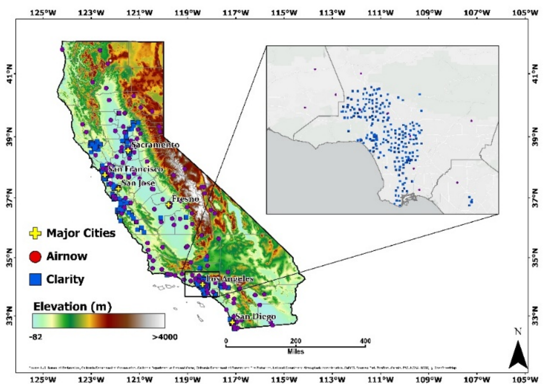
Figure 2.
Spatial distribution of AirNow (red circles) and Clarity (blue squares) PM₂.₅ monitoring sites in the Northeast United States, with elevation (m) shown as background shading.
Figure 2.
Spatial distribution of AirNow (red circles) and Clarity (blue squares) PM₂.₅ monitoring sites in the Northeast United States, with elevation (m) shown as background shading.
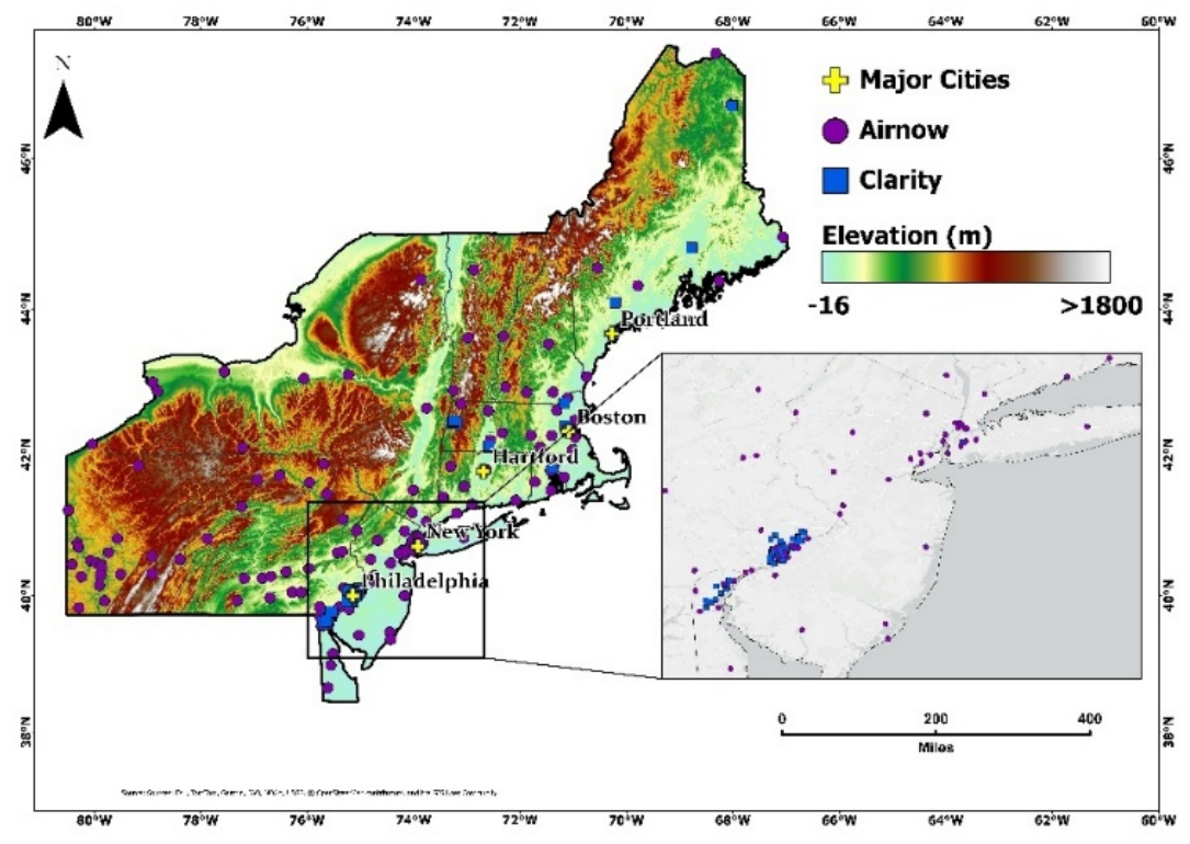
Figure 3.
Workflow of PM₂.₅ sensor calibration and uncertainty evaluation, including data acquisition, collocation, preprocessing, Transformer-based calibration, uncertainty estimation, and reliability assessment.
Figure 3.
Workflow of PM₂.₅ sensor calibration and uncertainty evaluation, including data acquisition, collocation, preprocessing, Transformer-based calibration, uncertainty estimation, and reliability assessment.
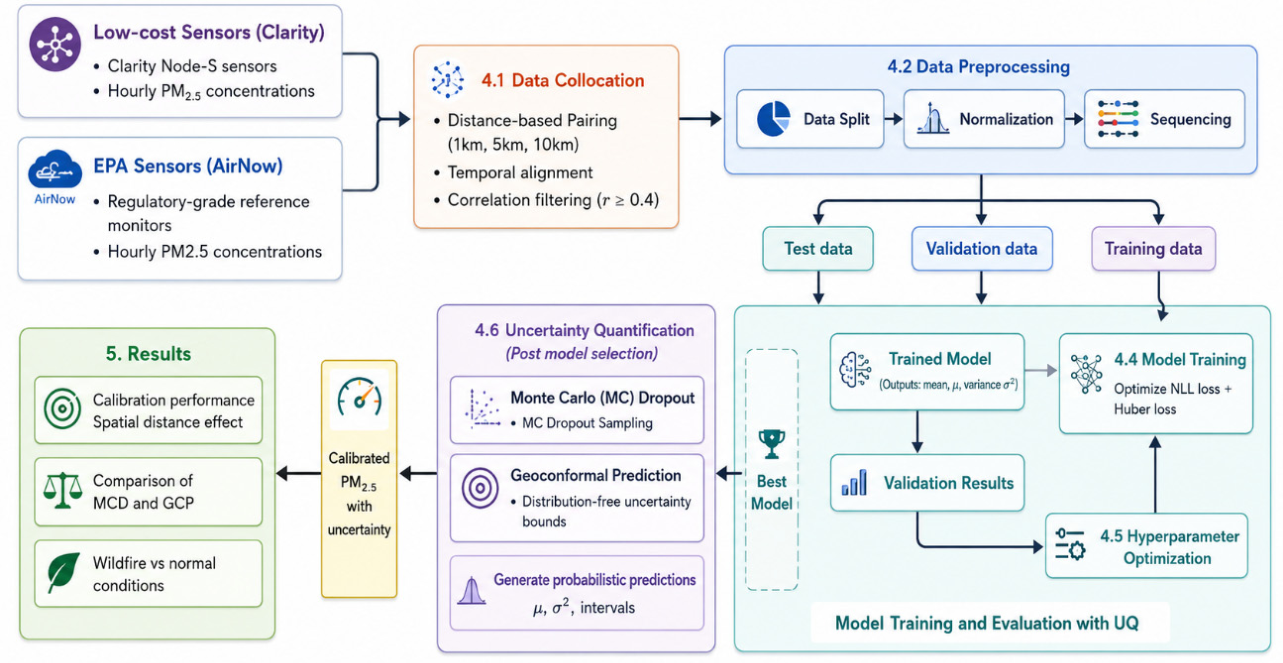
Figure 4.
Transformer-based calibration architecture for PM₂.₅ estimation with encoder–decoder attention mechanisms, and Monte Carlo dropout for UQ. .
Figure 4.
Transformer-based calibration architecture for PM₂.₅ estimation with encoder–decoder attention mechanisms, and Monte Carlo dropout for UQ. .
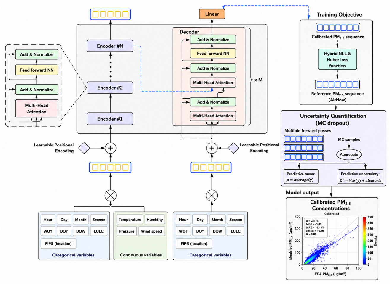
Figure 5.
Box plots of PM₂.₅ concentrations for AirNow and Clarity sensor pairs at (a) 1 km, (b) 5 km, and (c) 10 km distance thresholds in California.
Figure 5.
Box plots of PM₂.₅ concentrations for AirNow and Clarity sensor pairs at (a) 1 km, (b) 5 km, and (c) 10 km distance thresholds in California.
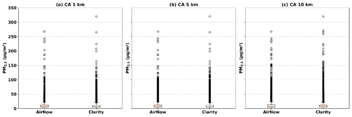
Figure 6.
Box plots of PM₂.₅ concentrations for AirNow and Clarity sensor pairs at (a) 1 km, (b) 5 km, and (c) 10 km distance thresholds in the Northeast.
Figure 6.
Box plots of PM₂.₅ concentrations for AirNow and Clarity sensor pairs at (a) 1 km, (b) 5 km, and (c) 10 km distance thresholds in the Northeast.
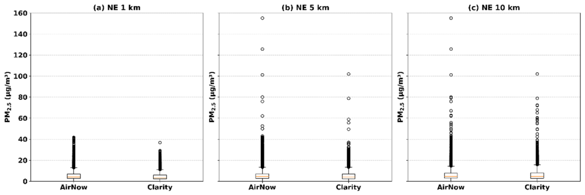
Figure 7.
PM₂.₅ concentration distributions for AirNow at (a) 1 km, (b) 5 km, and (c) 10 km, and Clarity at (d) 1 km, (e) 5 km, and (f) 10 km distance thresholds in California.
Figure 7.
PM₂.₅ concentration distributions for AirNow at (a) 1 km, (b) 5 km, and (c) 10 km, and Clarity at (d) 1 km, (e) 5 km, and (f) 10 km distance thresholds in California.
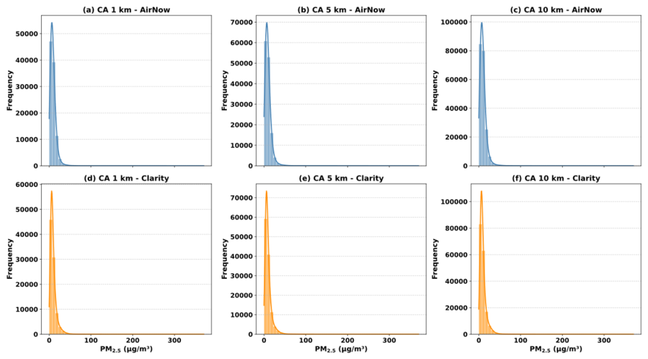
Figure 8.
PM₂.₅ concentration distributions for AirNow at (a) 1 km, (b) 5 km, and (c) 10 km, and Clarity at (d) 1 km, (e) 5 km, and (f) 10 km distance thresholds in California.
Figure 8.
PM₂.₅ concentration distributions for AirNow at (a) 1 km, (b) 5 km, and (c) 10 km, and Clarity at (d) 1 km, (e) 5 km, and (f) 10 km distance thresholds in California.
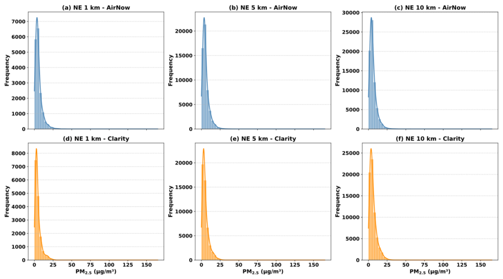
Figure 9.
Scatter plots of LCS PM₂.₅ vs. EPA PM₂.₅ for (a) uncalibrated and (b) calibrated Clarity sensors at the 1 km distance threshold in California.
Figure 9.
Scatter plots of LCS PM₂.₅ vs. EPA PM₂.₅ for (a) uncalibrated and (b) calibrated Clarity sensors at the 1 km distance threshold in California.
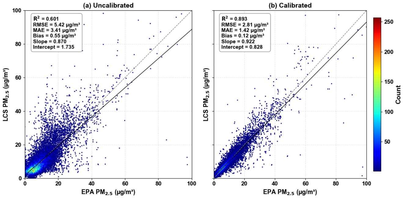
Figure 10.
Scatter plots of LCS PM₂.₅ vs. EPA PM₂.₅ for (a) uncalibrated and (b) calibrated Clarity sensors at the 1 km distance threshold in the Northeast United States.
Figure 10.
Scatter plots of LCS PM₂.₅ vs. EPA PM₂.₅ for (a) uncalibrated and (b) calibrated Clarity sensors at the 1 km distance threshold in the Northeast United States.
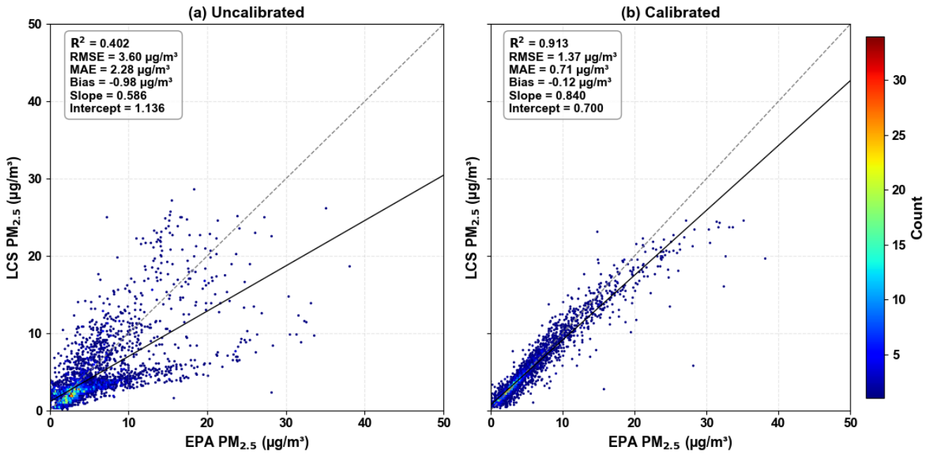
Figure 11.
Calibration curves for MCD (a) and GCP (b) uncertainty estimates in California. The red dashed line denotes perfect calibration; the blue curve shows observed coverage, with the shaded area representing the miscalibration area.
Figure 11.
Calibration curves for MCD (a) and GCP (b) uncertainty estimates in California. The red dashed line denotes perfect calibration; the blue curve shows observed coverage, with the shaded area representing the miscalibration area.
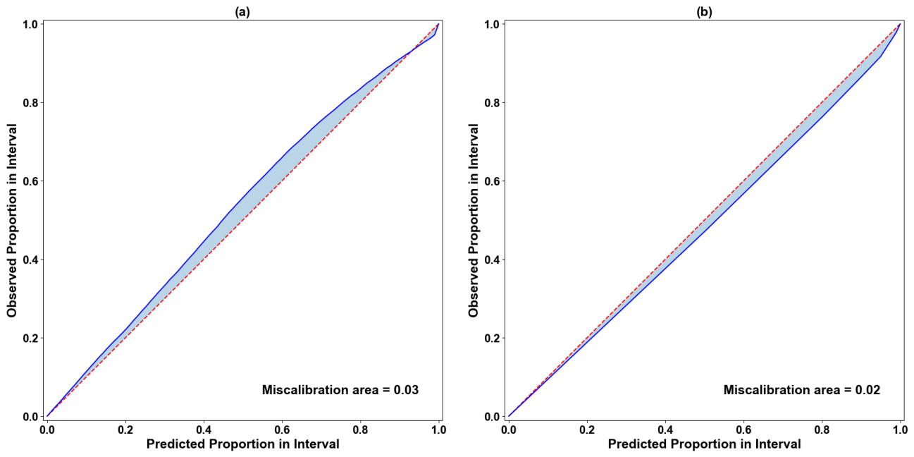
Figure 12.
Calibration curves for MCD (a) and GCP (b) uncertainty estimates in the Northeastern United States. The red dashed line denotes perfect calibration; the blue curve shows observed coverage, with the shaded area representing the miscalibration area.
Figure 12.
Calibration curves for MCD (a) and GCP (b) uncertainty estimates in the Northeastern United States. The red dashed line denotes perfect calibration; the blue curve shows observed coverage, with the shaded area representing the miscalibration area.
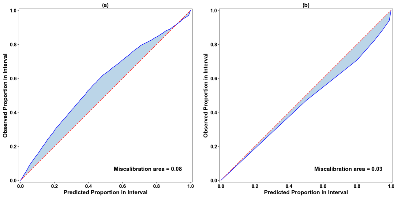
Figure 13.
Time-series calibration of Clarity PM₂.₅ against AirNow ground truth for wildfire events in California (a–c) at 29.40 m and the Northeast (d–f) at 6,798.84 m spatial separation at a 95% nominal prediction interval, showing (a, d) before calibration, (b, e) after calibration with MCD, and (c, f) after calibration with GCP.
Figure 13.
Time-series calibration of Clarity PM₂.₅ against AirNow ground truth for wildfire events in California (a–c) at 29.40 m and the Northeast (d–f) at 6,798.84 m spatial separation at a 95% nominal prediction interval, showing (a, d) before calibration, (b, e) after calibration with MCD, and (c, f) after calibration with GCP.
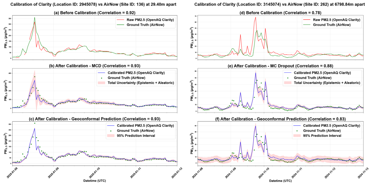
Figure 14.
Time-series calibration of Clarity PM₂.₅ against AirNow ground truth for a normal day in California (a–c) at 2.92 m and the Northeast (d–f) at 83.69 m spatial separation at a 95% nominal prediction interval, showing (a, d) before calibration, (b, e) after calibration with MCD, and (c, f) after calibration with GCP.
Figure 14.
Time-series calibration of Clarity PM₂.₅ against AirNow ground truth for a normal day in California (a–c) at 2.92 m and the Northeast (d–f) at 83.69 m spatial separation at a 95% nominal prediction interval, showing (a, d) before calibration, (b, e) after calibration with MCD, and (c, f) after calibration with GCP.
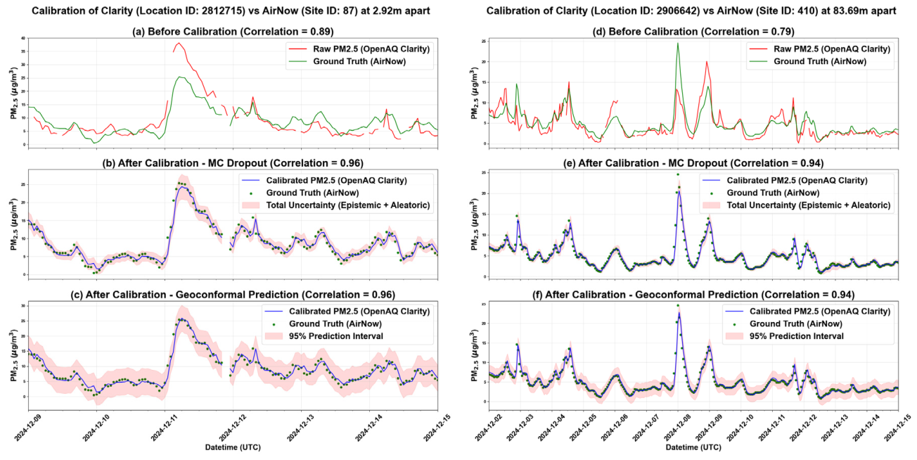
Figure 15.
Spatial distribution of GCP-derived geospatial uncertainty (µg/m³) across California sensor locations at the 1 km distance threshold.
Figure 15.
Spatial distribution of GCP-derived geospatial uncertainty (µg/m³) across California sensor locations at the 1 km distance threshold.
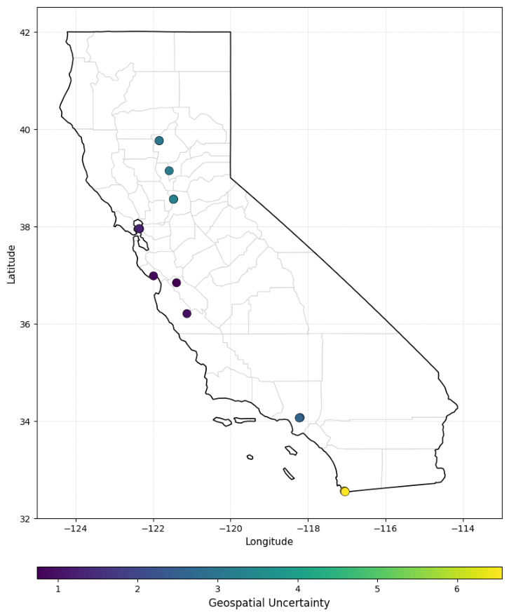

Table 1.
Summary of spatiotemporal collocation statistics for Clarity and AirNow sensor pairs across three distance thresholds (1 km, 5 km, and 10 km) in California and the Northeast United States.
Table 1.
Summary of spatiotemporal collocation statistics for Clarity and AirNow sensor pairs across three distance thresholds (1 km, 5 km, and 10 km) in California and the Northeast United States.
| Metric | NE 1km | NE 5km | NE 10km | CA 1km | CA 5km | CA 10km |
|---|---|---|---|---|---|---|
| Total pairs | 4 | 11 | 19 | 11 | 17 | 27 |
| Mean distance (m) | 48.8 | 1,476.1 | 3,843.7 | 117.9 | 1,132.4 | 3,604.5 |
| Max distance (m) | 83.7 | 4,104.2 | 9,717.7 | 464.4 | 4,164.0 | 9,892.9 |
| Mean correlation | 0.87 | 0.85 | 0.81 | 0.80 | 0.78 | 0.77 |
| Min correlation | 0.75 | 0.67 | 0.65 | 0.52 | 0.52 | 0.52 |
| Max correlation | 0.96 | 0.96 | 0.96 | 0.95 | 0.95 | 0.95 |
| Pairs with r > 0.7 | 4 | 10 | 16 | 9 | 13 | 20 |
| Pairs with r > 0.9 | 2 | 4 | 4 | 2 | 2 | 2 |
Table 2.
Optimized hyperparameters selected via random search for each region and spatial distance threshold.
Table 2.
Optimized hyperparameters selected via random search for each region and spatial distance threshold.
| Parameter | CA 1km | NE 1km | CA 5km | NE 5km | CA 10km | NE 10km |
| Epochs | 20 | 35 | 20 | 35 | 20 | 32 |
| Batch Size | 64 | 64 | 128 | 128 | 128 | 128 |
| Embedding Dimension | 256 | 256 | 512 | 512 | 512 | 512 |
| Dropout | 0.1 | 0.2 | 0.1 | 0.2 | 0.1 | 0.2 |
| Learning Rate | 1×10⁻⁴ | 1×10⁻⁴ | 3×10⁻⁴ | 3×10⁻⁴ | 3×10⁻⁴ | 2×10⁻⁴ |
Table 3.
Model performance metrics across three spatial distance thresholds (1 km, 5 km, and 10 km) for train and test splits in California.
Table 3.
Model performance metrics across three spatial distance thresholds (1 km, 5 km, and 10 km) for train and test splits in California.
| Distance Threshold | Split | R² | RMSE (µg/m³) | MSE (µg/m³) | MAE (µg/m³) | Bias (µg/m³) |
| 1 km | Train | 0.91 | 2.33 | 5.45 | 1.20 | -0.0013 |
| Test | 0.89 | 2.81 | 8.06 | 1.44 | 0.1075 | |
| 5 km | Train | 0.90 | 2.64 | 6.97 | 1.26 | -0.0140 |
| Test | 0.88 | 3.27 | 10.72 | 1.55 | -0.2474 | |
| 10 km | Train | 0.85 | 3.08 | 9.49 | 1.25 | -0.0196 |
| Test | 0.84 | 4.17 | 17.42 | 1.74 | 0.2606 |
Table 4.
Model performance metrics across three spatial distance thresholds (1 km, 5 km, and 10 km) for train and test splits in the Northeast United States.
Table 4.
Model performance metrics across three spatial distance thresholds (1 km, 5 km, and 10 km) for train and test splits in the Northeast United States.
| Distance Threshold | Split | R² | RMSE (µg/m³) | MSE (µg/m³²) | MAE (µg/m³) | Bias (µg/m³) |
| 1 km | Train | 0.95 | 1.03 | 1.06 | 0.60 | -0.0047 |
| Test | 0.91 | 1.38 | 1.90 | 0.71 | -0.1245 | |
| 5 km | Train | 0.94 | 1.19 | 1.41 | 0.64 | -0.0018 |
| Test | 0.88 | 1.63 | 2.66 | 0.76 | -0.3200 | |
| 10 km | Train | 0.92 | 1.31 | 1.72 | 0.58 | -0.0104 |
| Test | 0.82 | 2.1 | 4.39 | 0.72 | -0.3073 |
Table 5.
Calibration and uncertainty interval metrics for MCD and GCP approaches across confidence levels at the 1-km distance threshold in California.
Table 5.
Calibration and uncertainty interval metrics for MCD and GCP approaches across confidence levels at the 1-km distance threshold in California.
| UQ approach | Confidence Level | PICP | PIW (µg/m³) | ECE | |
|---|---|---|---|---|---|
| Ideal | Observed | ||||
| MCD | 50% | 0.50 | 0.55 | 2.37 | 0.02 |
| 80% | 0.80 | 0.83 | 4.52 | ||
| 90% | 0.90 | 0.91 | 5.80 | ||
| 95% | 0.95 | 0.94 | 6.93 | ||
| 99% | 0.99 | 0.97 | 9.12 | ||
| GCP | 50% | 0.50 | 0.47 | 1.67 | 0.03 |
| 80% | 0.80 | 0.76 | 3.46 | ||
| 90% | 0.90 | 0.86 | 4.91 | ||
| 95% | 0.95 | 0.92 | 6.55 | ||
| 99% | 0.99 | 0.98 | 12.90 |
Table 6.
Calibration and uncertainty-interval metrics for MCD and GCP approaches across confidence levels at the 1 km distance threshold in the Northeast.
Table 6.
Calibration and uncertainty-interval metrics for MCD and GCP approaches across confidence levels at the 1 km distance threshold in the Northeast.
| UQ approach | Confidence Level | PICP | PIW (µg/m³) | ECE | |
|---|---|---|---|---|---|
| Ideal | Observed | ||||
| MCD | 50% | 0.50 | 0.67 | 1.23 | 0.06 |
| 80% | 0.80 | 0.86 | 2.35 | ||
| 90% | 0.90 | 0.91 | 3.02 | ||
| 95% | 0.95 | 0.94 | 3.60 | ||
| 99% | 0.99 | 0.97 | 4.74 | ||
| GCP | 50% | 0.50 | 0.47 | 0.66 | 0.06 |
| 80% | 0.80 | 0.71 | 1.48 | ||
| 90% | 0.90 | 0.82 | 2.32 | ||
| 95% | 0.95 | 0.88 | 3.28 | ||
| 99% | 0.99 | 0.94 | 6.01 |
Table 7.
Summary of MCD and GCP uncertainty band behavior and ground truth coverage at the 95% confidence level under wildfire and normal conditions in California and the Northeast United States.
Table 7.
Summary of MCD and GCP uncertainty band behavior and ground truth coverage at the 95% confidence level under wildfire and normal conditions in California and the Northeast United States.
| Condition | Region | Distance | MCD Band | MCD Coverage | GCP Band | GCP Coverage |
|---|---|---|---|---|---|---|
| Wildfire | California | 29.40 m | Expands at spike | 69/97 (71%) | Stays narrow | 59/97 (61%) |
| Wildfire | Northeast | 6,798.84 m | Stays narrow | 53/121 (44%) | Expands | 100/121 (83%) |
| Normal | California | 2.92 m | Narrow, efficient | 117/145 (81%) | Wider throughout | 140/145 (97%) |
| Normal | Northeast | 83.69 m | Narrow, efficient | 229/313 (73%) | Wider throughout | 288/313 (92%) |
Table 8.
Comparison of this study with recent low-cost PM₂.₅ sensor calibration studies.
| Study | Study Area | Sensor | Model | R2 | RMSE | Wildfire | UQ applied? | Notes |
|---|---|---|---|---|---|---|---|---|
| This study | CA/NE | Clarity, AirNow | Transformer | 0.87/0.91 | 3.04/1.38 | Yes | Yes | Evaluates reliability under wildfire and spatial shift |
| [38] | Sofia, Bulgaria | AirThings + reference | Random Forest | 0.75 | 6.3 | No | Distance-based UQ | Spatial uncertainty increases with distance |
| [64] | India | CMOS LCS | GNN | 0.93 | 4.2 | No | NA | Strong ML calibration performance |
| [65] | Norway | Mobile LCS | XGBoost | 0.78 | 3.97 | No | Variability-based | Descriptive uncertainty only |
| [12] | South Korea | SPS 30 | Hybrid LSTM | 0.93 | ~3 | No | No | High calibration accuracy only |
| [29] | USA (CA, UT wildfires) | PurpleAir + reference | Adjustment factors | NA | NA | Yes | No | Wildfire-specific calibration |
Disclaimer/Publisher’s Note: The statements, opinions and data contained in all publications are solely those of the individual author(s) and contributor(s) and not of MDPI and/or the editor(s). MDPI and/or the editor(s) disclaim responsibility for any injury to people or property resulting from any ideas, methods, instructions or products referred to in the content. |
© 2026 by the authors. Licensee MDPI, Basel, Switzerland. This article is an open access article distributed under the terms and conditions of the Creative Commons Attribution (CC BY) license (http://creativecommons.org/licenses/by/4.0/).
Copyright: This open access article is published under a Creative Commons CC BY 4.0 license, which permit the free download, distribution, and reuse, provided that the author and preprint are cited in any reuse.


