

Submitted:
01 June 2026
Posted:
03 June 2026
You are already at the latest version
Abstract
The classical radius of convergence provides a definitive geometric boundary for the validity of a power series, yet it offers little insight into the actual efficiency of the approximation at a specific point. This paper introduces the concept of sequential radii of convergence to bridge the gap between the qualitative "where" of convergence and the quantitative "how fast" of partial-sum approximation. By defining the indexed radius—which measures the number of terms required to meet a prescribed error tolerance—and the geometric radius, we provide a framework for evaluating the computational cost of series representations. We categorize power series into three fundamental tail-decay regimes: sublinear, linear, and superlinear. Within this taxonomy, we derive explicit asymptotic formulas that reveal how the speed of convergence is influenced by both the coefficient growth and the evaluation point’s proximity to the boundary of the convergence disk. Furthermore, we investigate the stability of these sequential radii under standard algebraic operations, including sums, products, and quotients. To demonstrate the practical utility of this refinement, we present a comprehensive catalog of classical series—ranging from the logarithmic and binomial series to more complex forms like the Lambert W0 and Jacobi theta-type series—analyzing their behavior through this new lens. Ultimately, this work offers a more granular perspective on power-series analysis, transforming the classical radius from a static boundary into a dynamic measure of analytic efficiency.
Keywords:
power series
; radius of convergence
; tail asymptotics
; convergence rate
MSC: Primary: 30B10; Secondary: 40A05, 40A25
1. Introduction
1.1. The Classical Radius of Convergence
A power series centered at has the form
Its classical radius of convergence determines the interval on which the series converges absolutely, while the boundary points require separate analysis. Thus (R) gives the first geometric description of the region where the formal series represents a genuine function. Various mathematicians have contributed to its formal definition and computation as follows:
Brook Taylor (1685–1731) played a central role in the early development of power-series representation through Taylor’s theorem, which expresses a sufficiently regular function by polynomial approximations near a point. Although the modern theory of convergence came later, Taylor’s work established the local expansion viewpoint that remains fundamental in analysis [1,2,3].
Jean le Rond d’Alembert (1717–1783) refined the study of infinite series through the ratio test. In the setting of a power series, this test gives the familiar computation
whenever the limit exists. This provided a practical way to determine the interval of convergence directly from successive coefficients [4].
Augustin-Louis Cauchy (1789–1857) gave the theory of infinite series a rigorous foundation through systematic use of limits and convergence tests. His root-test viewpoint connects convergence to the exponential size of the coefficients and leads naturally to formulas involving . This shifted the theory from formal manipulation of series toward asymptotic control of coefficient growth [5,6].
Niels Henrik Abel (1802–1829) clarified one of the most delicate issues in the theory of power series: the relation between convergence inside the interval and limiting behavior at the boundary. Abel’s theorem shows, in particular, that when a power series converges at an endpoint, its sum is approached by the values of the series from inside the interval [7]. This result gave a precise form to the boundary question that remains outside the direct information provided by the radius R itself.
Jacques Hadamard (1865–1963) completed the modern coefficient-growth formulation through what is now called the Cauchy–Hadamard formula:
with the conventions and . This is the form most commonly used today when the ordinary ratio limit does not exist, since the lim sup captures the upper exponential growth rate of the coefficient sequence. In this sense, the classical radius is determined by the asymptotic size of the coefficients, and the Cauchy–Hadamard formula gives the standard bridge between coefficient growth and the geometry of convergence [5,8,9].
1.2. Motivation
The classical radius of convergence is one of the central organizing notions in the theory of power series. It gives a sharp geometric description of the interval, or disk in the complex setting, on which the series converges. In this sense, the classical radius answers the first natural question: where does the power series converge?
However, convergence is not only a question of location. Once a point (x) lies inside the interval of convergence, a second question becomes natural: how many terms are required before the partial sums approximate within a prescribed tolerance ? The classical radius R does not answer this question. It determines the domain of convergence, but it does not quantify the computational cost of convergence inside that domain.
This distinction is visible even among standard power series. Two series may have the same classical radius, while their tails decay at very different speeds. A geometric tail, an algebraically corrected geometric tail, and a factorial tail may all arise from familiar analytic functions, but they lead to different approximation costs. Thus, the usual classification by the classical radius alone does not fully describe the practical behavior of partial-sum approximation.
Standard references on analysis and power series usually emphasize convergence tests, endpoint behavior, uniform convergence on compact subintervals, and analytic continuation. These tools are fundamental, but they mainly describe qualitative convergence. They do not systematically attach to a power series a pointwise quantitative radius measuring the entry index into an -tube around the limiting value [4,5,8,9].
The purpose of this paper is to fill this gap by introducing sequential radii of convergence for power series. The indexed radius measures the number of terms required to reach accuracy at a fixed point x, while the geometric radius gives a reciprocal efficiency scale. Together, these quantities refine the classical radius by separating where a power series converges from how efficiently its partial sums converge there.
1.3. Organization of the Paper
This paper is organized as follows. Section 2 reviews the mathematical background needed for the sequel, including classical convergence, tail remainders, indexed and geometric radii for sequences, and the associated tail-classification theorem. Section 3 develops the theory of sequential radii of convergence for power series in the space , viewed as a natural extension of the corresponding theory for numerical sequences. First, Section 3.1 introduces the sequential radii of convergence for power series, proves the main classification theorem, and defines the three associated tail-class subspaces of . Second, Section 3.2 describes the geometry of the sequential radii, emphasizing both the indexed and geometric viewpoints. Third, Section 3.3 studies the behavior of sequential radii under algebraic operations. Fourth, Section 3.4 presents a catalog of examples and explicit computations for two important tail-class subclasses of : the linear and superlinear regimes. Finally, Section 4 concludes the paper by summarizing its main contributions, discussing its limitations, and outlining possible directions for future work.
2. Preliminaries
The reader who has studied real analysis is well acquainted with the following background theory of sequences and series [4,5,6,10]:
2.1. Classical Convergence and Tail Remainders
Definition 1
(Series)). Given a sequence of real numbers, its associated series is the symbolic sum Its Nth partial sum is and the tail reminder is . The series converges to s if and in this case we write ; otherwise, the series diverges.
Definition 2
(Power Series). Given a sequence of real coefficients and a center , a power series around a is a series of the form Furthermore, its tail is defined by Its convergence depends on x, and the set of convergence is described by a radius of convergence around the center a.
Definition 3
(Taylor Series). A Taylor series is a power series whose coefficients are determined by the derivatives of a infinitely differentiable function f at a center given by
Definition 4
(Space of Real Power Series at a Center). For a fixed center , let denote the set of all real power series with classical radius of convergence . For with coefficient sequences and , respectively, and for , the following operations are defined on the common open interval of convergence :
- 1.
- Scalar multiplication. .
- 2.
- Sum and difference. .
- 3.
- Pointwise product. , defined as the ordinary product of values on the common interval of convergence. As a function, coincides with the Cauchy product (cf. item 5 below).
- 4.
- Synchronized product approximants. For each , set and The sequence is a polynomial approximant of degree to and is, in general, distinct from the Cauchy partial sums of , which have degree n.
- 5.
- Cauchy product. , where .
- 6.
- Hadamard product. .
- 7.
- Quotient. When , the quotient is well-defined on a neighborhood of a.
- 8.
- Termwise differentiation and integration. and .
- 9.
- Argument transformations. For and , and .
Remark 1
(Distinction among the three products). The pointwise product , the Cauchy product , and the Hadamard product coincide as formal power series only in degenerate cases, and in general they produce distinct coefficient structures and distinct sequential radii of convergence [4,11]. This distinction is essential in Section 3.3 (cf. Remark 6).
Theorem 1
(Classical Convergence Tests for Series). Let be a series.
- 1.
-
Cauchy’s Root Test. DefineIf , then converges absolutely; if , then diverges; and if , the test is inconclusive.
- 2.
-
d’Alembert’s Ratio Test. Suppose eventually and defineIf , then converges absolutely; if , then diverges; and the borderline case is inconclusive.
Theorem 2
(Classical Radius of Convergence for a Power Series). Let be a real power series. Define Then the classical radius of convergence is with the conventions and . Hence converges absolutely for and diverges for . The endpoint cases when , must be checked separately. If, moreover, the ratio limit exists, then equivalently
Remark 2
(Classical radius dependency on spatial position ). Let be a real power series, with associated tail and classical radius of convergence Then, inside the convergence interval, the asymptotic cost of making the tail small depends on how fast the remainder decays. In particular, the position x plays an essential role only in the genuinely geometric case, where the effective ratio is comparable to (See Table 1).
Theorem 3
(The Stirling’s Approximation). For any positive integer n, as :
Theorem 4
(Asymptotic Expansion of Harmonic Numbers). Let denote the n-th harmonic number, and let be the Euler–Mascheroni constant. As , the partial sums satisfy the logarithmic approximation:
Theorem 5
(Euler Number Asymptotic Formula). Let denote the even-indexed Euler numbers. As , the growth rate of the normalized coefficients satisfies the asymptotic behavior:
Theorem 6
(Bernoulli Number Asymptotic Formula). Let denote the even-indexed Bernoulli numbers, and let . Then, the asymptotic behavior is given by:
Theorem 7
(Hardy–Ramanujan Asymptotic Formula). Let denote the number of partitions of a positive integer n. As , the partition function satisfies the asymptotic behavior:
2.2. The Indexed Radius of Convergence and Tail Errors
The following notions are adapted from the indexed, geometric, and Cauchy radii introduced for numerical series in [10,12]. They are recalled here in a self-contained form, since the power-series construction in Section 3 is obtained by applying them pointwise to the associated tail sequence .
Definition 5
(Indexed Radius of convergence of a series). Let be a real series, and let denote its N-th partial sum. Suppose that the partial sums have limit . For , define the radius of convergence of s at level ε by
where
Definition 6
(Geometric radius of convergence of a series). Let be a real series, and let denote its index-radius of convergence at level . To emphasize the analogy with geometric notions of radius, one may equivalently work with the rescaled radius
with the convention .
Definition 7
(Cauchy radius of a series). Let be a real series, and let denote its N-th partial sum. For , define the Cauchy radius of s at level ε by
where
Theorem 8
(Tail-Inversion Principle for Series). Let be a convergent real series with finite sum . Let denote the partial sums and the corresponding tails. Suppose that there exists a strictly decreasing, continuous, and invertible function such that Then,
- (i)
- (ii)
Corollary 1
(Tail-decay classes and induced convergence radii). Let be a convergent real series with finite sum . For , write Let and denote, respectively, the index-radius and the geometric radius of convergence of the partial-sum sequence . As , the asymptotic decay of the tail determines the corresponding radius class as summarized in Table 2.
3. Theory of Sequential Radii of Convergence for Power Series
The preceding section recalled the indexed and geometric radii for numerical series. We now transfer this point of view to power series by fixing an evaluation point inside the classical interval of convergence and applying the numerical theory to the corresponding tail sequence This pointwise reduction is the basic mechanism behind the sequential radii of convergence for power series.
3.1. The General Classification Theorem
Definition 8
(Indexed radius of convergence of a power series). Let be a power series, and for each define the N-th partial sum and tail by For a fixed x at which the power series converges to , and for , define the indexed radius of convergence at x by
Remark 3
(Geometric and Cauchy radii for a power series). Let and For a fixed and , the following two associated radii are useful.
- 1.
-
Geometric radius. If denotes the indexed radius of convergence of the power series at x, definewith the convention .
- 2.
-
Cauchy radius. Define the Cauchy radius of the power series at x bywhere
Definition 9
(Sequential Radii of Convergence for power series). Let be a power series, and We refer to the pair as its sequential radii at given fixed point .
Theorem 9
(Sequential Radii of Convergence for Power Series). Let be a power series with classical radius of convergence . Fix x with , and define its associated nth partial sum and tail respectively. Assume that, as , the tail belongs to one of the following decay regimes. Then, as , the corresponding indexed and geometric radii are given by
In particular, in the linear regime, the spatial dependence of the indexed radius enters through the classical relative position If , then for all , and therefore respectively.
Proof.
Fix x with , and set Then and its n-th tail is exactly Hence the indexed radius is precisely the indexed radius of the fixed numerical series . The three asymptotic formulas for therefore follow directly from Corollary 1 applied to the numerical tail . The formulas for the geometric radius follow from the definition in Remark 3. Finally, in the linear power-series regime, the decay ratio is the relative distance of x from the center of expansion, namely which gives the stated spatial dependence. The case is immediate, since all powers vanish for , so the tail is identically zero. □
Theorem 9 identifies three model regimes for the decay of the tail It is therefore natural to separate those power series whose tails fall into one of these regimes at a fixed point The following definition records this separation as a tail-class decomposition inside the space
Definition 10
(Tail-class subspaces of ). Fix a center , and let be the space of real power series centered at a in the sense of Definition 4. Thus where denotes the classical radius of convergence of f. For , define the N-th partial sum and tail by and respectively. For a fixed point x at which the power series converges, define the following tail-class subspaces of :
The corresponding tail-class decomposition is therefore:
Here, denotes the subclass of power series in whose tail at the fixed evaluation point x belongs to one of the three model regimes appearing in Theorem 9.
Remark 4
(Structural Consequences). Theorem 9 has several immediate consequences as follows:
- (a)
- Interpretation of the tail constant C: The constant C is the leading amplitude of the tail asymptotic , where , , or in the sublinear, linear, and superlinear regimes, respectively. While C is crucial for calculating the exact error at a specific index the Theorem shows that C is irrelevant for the asymptotic growth rate of the sequential radii of convergence. Figure 1(a) visualizes that changing shifts the indexed radius curve but does not change the asymptotic growth rate order.
- (b)
- Convergence-speed Classification: The Theorem classifies sequential convergence by the decay of the geometric radius : sublinear tails give a polynomial scale , linear tails give the logarithmic scale , and superlinear tails give the faster efficiency scale . Thus the table separates polynomial, geometric, and factorial tail behavior into three distinct radius classes, while in all nondegenerate cases as , reflecting the continuous narrowing of the admissible geometric window. Figure 1(b) compares the three radius classes: polynomial/sublinear, logarithmic/linear, and factorial/superlinear.
- (c)
- Geometry of Sequential Convergence: The spatial geometry of the Theorem appears explicitly in the linear regime through , where . Thus convergence is fastest near the center , where the tail is degenerate, and becomes arbitrarily slow as , reflecting the increasing cost of approximation near the boundary of the classical disk of convergence. Figure 1(c) shows the explosion of the indexed radius as approaches the boundary
3.2. The Geometry of the Sequential Radii
The preceding section summarized the structural consequences of Theorem 9, including the role of the tail constant, the separation of convergence-speed classes, and the spatial dependence of the linear regime. The last of these is intrinsically geometric, since the sequential radii depend on the relative position inside the classical interval of convergence. While Figure 1(c) showed this dependence along a one-dimensional radial slice, the present section lifts the same phenomenon to a two-dimensional surface over x and .
Figure 2 further illustrates the two-dimensional geometry induced by the linear regime of Theorem 9. In this regime, with , , and , the indexed radius has the asymptotic form
Panel (a) shows the corresponding indexed-radius surface over the spatial variable x and the precision scale . The surface has a funnel-like geometry: near the center , the approximation cost is small because the tail is degenerate at the center of expansion, while the indexed radius grows increasingly fast as approaches the boundary . Thus the same tolerance requires substantially more terms near the edge of the classical interval of convergence than near the center. This visualizes the spatial dependence encoded in the denominator , which becomes small as .
Panel (b) displays the associated geometric radius
This surface gives the reciprocal geometric interpretation of the same phenomenon. While the indexed radius measures the number of terms required for a given accuracy, the geometric radius measures the corresponding normalized efficiency scale. Hence the surface is largest near the center of expansion, where convergence is most efficient, and it collapses toward zero both as the precision demand increases and as x moves toward the boundary of convergence. Together, the two panels show that the linear regime is not only a tail-decay class, but also a spatial geometry: convergence becomes progressively more expensive as the evaluation point approaches the classical boundary .
3.3. Algebraic Operations
The preceding sections studied the sequential radii of a single power series through the decay of its tail sequence. We now record how these radii behave under elementary algebraic operations. The point of view is local in the evaluation point x: after fixing x inside the common interval of convergence, each power series gives a convergent sequence of partial sums, and the algebraic operations reduce to corresponding operations on these partial-sum sequences. Thus the estimates below should be read as stability bounds for the computational cost of approximation under scalar multiplication, addition, multiplication, and division.
Throughout this subsection, fix a center and consider two power series , with and and classical radii of convergence and , respectively. For each , denote their n-th partial sums and tails by and and analogously , , and let , denote the associated indexed radii in the sense of Definition 5. Throughout, x is fixed in the common open interval of convergence . Under this notation, the following theorem records the stability of the sequential radii under the algebraic operations of Definition 4. We use this notation in the following Theorem:
Theorem 10
(Algebraic stability of sequential radii). Let f and g be two real power series with common center a, and fix x in the common open interval of convergence. Then the following estimates hold for every .
- (i)
- Scalar multiplication. Let and . If , then If , then and
- (ii)
- Sum and difference. Let . Then More generally, for every , we have
- (iii)
- Pointwise product of synchronized approximants. Define the synchronized product approximants by and Let Then where denotes the indexed radius associated with the approximating sequence .
- (iv)
- Quotient. Assume . Define the synchronized quotient approximants by and Then for all sufficiently large n, and For every , set Then
Proof.
The proof is divided according to the listed assertions. Fix x in the common open interval of convergence. Then and and the indexed radii and are precisely the entry indices of these two partial-sum sequences into their corresponding -tubes.
(i). For scalar multiplication, if , then Hence if and only if when , which gives the stated identity. If , the tail is identically zero, so the radius is 0.
(ii). For sums and differences, write . Then, Therefore, if then Taking gives the symmetric estimate.
(iii). For the synchronized product, write
If then and Since , we obtain
This proves the product estimate.
(iv). Finally, assume . We accomplish the proof in few steps as in follows.
Step 1. We consider the synchronized quotient approximants and Since , the denominators are eventually nonzero. More precisely, if then, by the reverse triangle inequality, Thus, whenever the tail error of g is smaller than , the denominator is bounded away from zero. Moreover, Using , we obtain and therefore
Step 2. Now write
Taking absolute values gives
Hence, by inequality (22)
Step 3. We now choose a common error tolerance that guarantees both the denominator condition and the final -bound. Define Let Then for every , we have and Accordingly, by inequality (23):
Therefore, and hence This proves the quotient estimate. □
Remark 5
(Interpretation of the algebraic bounds). The estimates in Theorem 10 show that algebraic operations do not destroy sequential convergence inside the common interval of convergence. Scalar multiplication simply rescales the tolerance. Sums and differences require both input tails to be small, so the resulting radius is controlled by the worse of the two entry indices. Products and quotients introduce dependence on the limiting values and , because the error propagation contains mixed terms. In this sense, the sequential radii behave like computational stability profiles for algebraic operations on power-series approximations.
Remark 6
(Pointwise vs. Cauchy vs. Hadamard multiplication). The following observations distinguish three notions of multiplication on power series.
- (a)
- The pointwise product and the Cauchy product coincide as functions on the common open interval of convergence, with shared coefficient structure . The Hadamard product is a genuinely distinct power series, with coefficients and limit generally different from .
- (b)
- Although and agree as functions, their natural approximating sequences differ. The synchronized pointwise approximants are , of degree , whereas the Cauchy-product partial sums are , of degree n. Both sequences converge to on the common interval of convergence, but enter the ε-tube at generally distinct indices. Hence their indexed and geometric radii are generally distinct.
- (c)
- For the Cauchy and Hadamard cases, the tails and both vanish on the respective intervals of convergence, so and for every . In general, however, no universal formula expresses or in terms of and alone; once an asymptotic estimate for the relevant tail is available, the corresponding radius follows from Theorem 9. Table 3 presents the list of counterexamples.

Table 3.
Counterexamples supporting Remark 3.8(c): twin pairs and exhibiting identical individual indexed radii but distinct product radii. Parameters: , ; asymptotics are stated as .
Table 3.
Counterexamples supporting Remark 3.8(c): twin pairs and exhibiting identical individual indexed radii but distinct product radii. Parameters: , ; asymptotics are stated as .
| (a) Cauchy product f ∗ g. | ||||||
|---|---|---|---|---|---|---|
| # | ||||||
| 1 | 1 | 0 | ||||
| 2 | ||||||
| (b) Hadamard product f ⊙ g. | ||||||
| # | ||||||
| 1 | 0 | 0 | ||||
| 2 | ||||||
Notes. Asymptotic equivalences (~) are taken in the sense of Theorem 9 applied to the appropriate tail; scaled exponential series fw(x) = ewx = ,
(w ≠ 0), has superlinear tail regime;
lacunary-type geometric series
fa,b(x) = = , (a, b > 0), has linear tail regime.
3.4. A Catalog of Classical Power Series: Examples and Explicit Sequential-Radius Computations
This section records a selected catalog of classical power series and computes their sequential radii in the sense of Definition 8 and Remark 3. This list is not exhaustive rather it is chosen to represent often historically important series expansions, different classical radii of convergence, and different coefficient structures. Throughout this subsection, the center is taken unless otherwise stated, and x is fixed in the interior of the classical interval of convergence. In the next two subsections, we use the preceding lemmas to identify general patterns in the tail behavior of our examples [6,13,14].
3.4.1. Linear/Geometric Series: Class 2
The series discussed in this section have finite classical radius we write The phrase "linear class" means that the tail is geometric up to subexponential or algebraic factors in the index. This assumption slightly broadens the strict hypothesis in Theorem 9, but only at lower order: factors such as or the sparsity of nonzero coefficients may contribute secondary corrections, while the leading indexed-radius remains as in Theorem 9. We start with the first key pattern lemma [12,16]:
Lemma 1
(Series Tail Pattern(1)). Let be a real power series with finite positive classical convergence radius Suppose, its tail satisfy:
where is a function, and Then:
Proof.
Set and Since , taking logarithms gives:
Moreover, and and therefore
We now invert this estimate in both directions. Fix and define At this scale , hence . Consequently, for sufficiently small . Thus . Since the geometric factor dominates the lower-order factors, the tail is eventually decreasing in magnitude, and therefore is an admissible entry index. Hence
For the reverse estimate, define Again , and hence for sufficiently small . Thus , so no index can be admissible. Therefore
Letting in (29) yields
□
Lemma 2
(Tail pattern for geometric series). Let be a real power series with finite positive classical radius of convergence Assume that the coefficients satisfy for some parameters Fix an interior point Then, as ,
Proof.
The proof is divided into several steps.
Step 1. For the fixed point x, write the n-th term of the power series as
Step 2. Since , the geometric factor dominates the algebraic, logarithmic, and subexponential factors in . In particular, for every fixed ,
This proves the claim. □
Example 1
(Lacunary geometric series). The lacunary geometric function has the power-series expansion Fix , and write Then This is the geometric pattern of Lemma 1 in the variable y, with Therefore By Lemma 2, the lacunary-index tail satisfies Equivalently, Thus, by Lemma 1,
Example 2
(Reciprocal square series). The reciprocal square function has the power-series expansion Thus the coefficient sequence is and therefore This is of the form in Lemma 2 with For fixed , we have and Hence, by Lemma 2, Therefore This is a linear/geometric tail with one algebraic factor. Applying Lemma 1, we obtain
Example 3
(Logarithm series). The logarithm function has the power-series expansion Equivalently, setting we may write Thus, in the variable y, the coefficient sequence satisfies This is of the form in Lemma 2 with For fixed , we have Therefore Hence, by Lemma 2, Therefore This is a linear/geometric tail with one algebraic factor . Applying Lemma 1, we obtain
Example 4
(Inverse hyperbolic tangent series). The inverse hyperbolic tangent function has the power-series expansion Fix , and write Then The coefficient sequence in the variable y satisfies Therefore this is of the form in Lemma 2 with For fixed , we have Thus After multiplying by the outer factor x, Lemma 2 gives Hence This is a lacunary linear/geometric tail with one algebraic factor . Applying Lemma 1, we obtain
Example 5
(Harmonic generating function series). The harmonic generating function has the power-series expansion where By Theorem 4, and therefore Thus the coefficient sequence satisfies This is of the form in Lemma 2 with For fixed , we have Therefore Hence, by Lemma 2, Consequently, This is a linear/geometric tail with one logarithmic correction. Applying Lemma 1, we obtain
Example 6
(Legendre chi series). The Legendre chi function has the power-series expansion Fix , and write Then The coefficient sequence in the variable y satisfies Therefore this is of the form in Lemma 2 with For fixed , we have Thus, After multiplying by the outer factor x, Lemma 2 gives Hence This is a lacunary linear/geometric tail with algebraic factor . Applying Lemma 1, we obtain
Example 7
(Arcsine series). The arcsine function has the power-series expansion Fix , and write Then Using the central-binomial asymptotic we obtain Thus the coefficient sequence in the variable y satisfies Therefore this is of the form in Lemma 2 with For fixed , we have Thus After multiplying by the outer factor x, Lemma 2 gives Hence This is a lacunary linear/geometric tail with algebraic factor . Applying Lemma 1, we obtain
Example 8
(Binomial series). The generalized binomial function has the power-series expansion where . Using the standard coefficient asymptotic we write Then the coefficient sequence in the variable y satisfies Therefore this is of the form in Lemma 2 with For fixed , we have Thus Hence, by Lemma 2, Consequently, This is a linear/geometric tail with algebraic factor . Applying Lemma 1, we obtain
Example 9
(Polylogarithm series). The polylogarithm function has the power-series expansion Here the summation starts from , since is not defined at . The coefficient sequence satisfies Therefore this is of the form in Lemma 2 with For fixed , we have Thus Hence, by Lemma 2, Consequently, This is a linear/geometric tail with algebraic factor . Applying Lemma 1, we obtain
Example 10
(Catalan generating function series). The Catalan generating function has the power-series expansion The coefficient sequence is [17]. Using the central-binomial asymptotic we obtain Therefore this is of the form in Lemma 2 with For fixed , we have Thus Hence, by Lemma 2, Consequently, This is a linear/geometric tail with algebraic factor . Applying Lemma 1, we obtain
Example 11
(Lambert series). The principal Lambert W-function has the power-series expansion [18]. Since we write Then Using Stirling’s approximation we obtain Thus the coefficient sequence in the variable y satisfies Therefore this is of the form in Lemma 2 with For fixed , we have Thus Hence, by Lemma 2, Consequently, This is a linear/geometric tail with algebraic factor . Applying Lemma 1, we obtain
Example 12
(Complete elliptic integral series). The complete elliptic integral of the first kind has the power-series expansion Fix , and write Then Using the central-binomial asymptotic we obtain Thus, before multiplying by the outer factor , the coefficient sequence in the variable y satisfies Therefore this is of the form in Lemma 2 with For fixed , we have Thus After multiplying by the outer factor , Lemma 2 gives Hence This is a lacunary linear/geometric tail with algebraic factor . Applying Lemma 1, we obtain
Example 13
(Secant function series). The secant function has the power-series expansion where denotes the Euler numbers. Using the Euler-number asymptotic Theorem 5 we obtain Fix , and write Then Thus the coefficient sequence in the variable y satisfies Therefore this is of the form in Lemma 2 with For fixed , we have Thus Hence, by Lemma 2, Consequently, This is a lacunary linear/geometric tail. Applying Lemma 1, we obtain
Example 14
(Tangent function series). The tangent function has the power-series expansion The term is zero, so the effective summation begins at . By Theorem 6, Therefore Fix , and write Reindexing by , we have The coefficient sequence in the variable y satisfies Thus this is of the form in Lemma 2 with For fixed , we have Thus After multiplying by the outer factor x, Lemma 2 gives Consequently, This is a lacunary linear/geometric tail. Applying Lemma 1, we obtain
Example 15
(Partition generating function series). The partition generating function has the power-series expansion where denotes the number of partitions of n [15,19]. By Theorem 7, Therefore the coefficient sequence satisfies This is of the form in Lemma 2 with For fixed , we have Thus Hence, by Lemma 2, Consequently, This is a linear/geometric tail with a subexponential correction. Applying Lemma 1, we obtain
Example 16
(Jacobi theta-type lacunary series). The Jacobi theta-type function has the lacunary power-series expansion [6,14]. Here the nonzero powers occur only at the square indices . Therefore the series is not directly of the coefficient-asymptotic form in Lemma 2, since the ordinary coefficient sequence has many zeros. Instead, the tail is computed from the square-lacunary structure. For fixed , define the lacunary-index tail by Since , the absolute size of the terms is governed by Moreover, Thus the terms decrease faster than geometrically in the lacunary index. Consequently, the tail is asymptotic to its first omitted term: Equivalently, The lacunary-index radius is therefore determined by Taking logarithms gives Hence Therefore
3.4.2. Superlinear/Entire Series: Class 3
The series discussed in this section have infinite classical radius These series are entire and their tail is superlinear, usually factorial or stronger [11,14]. We start with the second key pattern lemma:
Lemma 3
(Series Tail Pattern(2)). Let be a real power series with infinite classical convergence radius Suppose, its tail satisfy:
where and Then:
Proof.
Set Taking logarithms in the assumed tail asymptotic gives
Since and the dominant term is . Thus the inequality is governed asymptotically by
We now invert this relation. Fix , and define At this scale, Moreover, and Therefore, for sufficiently small . Hence Since the model tail is eventually decreasing, is an admissible entry index. Consequently,
For the reverse estimate, define Then and again the remaining terms are . Hence for sufficiently small . Therefore so no index below this scale can be admissible. Thus
Letting in (39), we obtain
This proves the result. □
Lemma 4
(Tail pattern for factorial-power entire series). Let where and Assume that where Then, for fixed , as , we have
Proof.
The proof is constituted of several steps as follows:
Step 1. Write
By assumption, Hence,
Step 3. It remains to compute the asymptotic form of . By approximation (42) and Stirling’s formula,
This proves the stated tail-format estimate. □
Example 17
(). The scaled exponential function has the power-series expansion This is of the form in Lemma 4 with Therefore Hence, for fixed , we have By Lemma 3,
Example 18
(). The sine function has the power-series expansion This corresponds to Therefore Hence By Lemma 3,
Example 19
(). The cosine function has the power-series expansion This corresponds to Therefore Hence By Lemma 3,
Example 20
(). The hyperbolic sine function has the power-series expansion This corresponds to Therefore Hence By Lemma 3,
Example 21
(). The hyperbolic cosine function has the power-series expansion This corresponds to Therefore Hence By Lemma 3,
Example 22
(). The error function has the power-series expansion This corresponds to Moreover, Thus Therefore Hence By Lemma 3,
Example 23
(). The Bessel function has the power-series expansion This corresponds to Moreover, Thus Therefore Hence By Lemma 3,
3.4.3. Catalog Summary Table
Table 4 presents the summary of examples presented in previous sections. We identify the patterns as follows:
3.4.3.1. Classical-radius ranges.
The catalog separates the examples into finite-radius and infinite-radius families. Within the linear/geometric class, the classical radius may be smaller than one, equal to one, or larger than one: the Catalan and Lambert series have , most logarithmic, polylogarithmic, binomial, lacunary, elliptic, partition, and theta-type examples have , while the trigonometric tangent and secant examples have . In contrast, the factorial-type examples in the superlinear class all have . Thus the classical radius records the domain of convergence, but it does not by itself determine the sequential cost; the same finite radius range may contain several different coefficient structures and lacunarity patterns.
3.4.3.2. Speed of the indexed radius.
For the linear/geometric examples, the indexed radius grows on the logarithmic scale up to constant factors caused by lacunarity, such as or . Algebraic, logarithmic, and subexponential coefficient corrections, such as , , or , affect the tail amplitude and lower-order behavior but do not change the leading logarithmic order. By contrast, the superlinear entire examples have factorial-type tails and therefore require only with constants such as distinguishing full factorial, even/odd factorial subsequences, and squared-factorial structures.
3.4.3.3. Overall findings.
The main lesson of the catalog is that the sequential radius refines the classical radius by measuring the approximation cost inside the convergence interval. Finite-radius series in the linear class can have very different coefficient origins—algebraic singularities, central-binomial coefficients, Bernoulli or Euler numbers, partition asymptotics, or lacunary supports—yet their leading indexed-radius behavior is governed by the same geometric mechanism. Entire factorial-type series form a separate, faster class: their infinite classical radius is accompanied by substantially smaller indexed radii. Hence the table shows that R tells where the power series converges, while describes how many terms are needed to converge at a prescribed accuracy.
0pt 0pt [longtable]width=
The preceding catalog shows that many classical examples fall into two tractable model families: geometric tails with lower-order corrections and factorial-type entire tails. For later tail-transfer computations, it is useful to isolate these two families as explicit subclasses of the broader linear and superlinear classes. The following definition records the subclasses on which the subsequent transformation analysis is intended to operate.
Definition 11
(Model subclasses for tail-transfer computations). Let be the space of real power series centered at 0, as in Definition 4. For , write and The tail-transfer computations below are carried out on the following two model subclasses of the tail classes introduced in Definition 10:
Remark 7 (Class Subsets).
The following chain of subsets hold using Lemma 1, Lemma 2, Lemma 3, Lemma 4 and Definition 10:
4. Discussion
The preceding sections introduced sequential radii for power series, established their basic classification, and computed them for a range of standard examples. We now summarize the main contributions of the paper, indicate the limitations of the present framework, and describe several directions in which the theory may be extended.
4.1. Summary and Contributions
This paper contributes to the theory of powers series in three dimensions as follows:
The first and the most prominent contribution of this paper is to complement the classical radius with the sequential radii and , which measure how many terms are needed to approximate the value of the series within a prescribed tolerance. In this sense, the sequential radius records a quantitative convergence profile rather than only a qualitative convergence domain. The classification theorem shows that the asymptotic behavior of the tail remainder induces three basic convergence-cost regimes. Sublinear tails lead to polynomial indexed radii, linear or geometric tails lead to logarithmic indexed radii, and superlinear or factorial tails lead to still faster logarithmic-over-logarithmic growth. Thus, the paper separates power series not only according to where they converge, but also according to how efficiently their partial sums approach the limiting value.
The second contribution is the geometric interpretation of the linear regime. In this case, the effective ratio shows explicitly how the evaluation point x affects the approximation cost. The indexed radius is small (i.e., low cost computationally) near the center of expansion and increases (i.e., higher cost computationally) as x approaches the boundary of the classical interval of convergence. This gives a geometric refinement of the classical radius: points inside the same convergence interval may have substantially different computational costs.
Finally, the paper records stability properties of the sequential radii under elementary algebraic operations and provides a catalog of classical examples. These examples show that many familiar power series fall naturally into the linear or superlinear tail classes. The resulting computations illustrate that the proposed radii are not merely formal definitions, but can be explicitly evaluated for standard analytic functions.
The results above show that sequential radii provide a useful quantitative refinement of the classical radius. At the same time, the present treatment is intentionally model-based, and its scope is limited by the tail regimes and pointwise setting considered here.
4.2. Limitations
The limitations of this work are clear. First, the present work focuses on model tail regimes. The three classes considered here capture several important patterns, but they do not exhaust all possible tail behaviors of convergent power series. More irregular tails, oscillatory remainders, mixed asymptotic scales, or slowly varying corrections may require refinements beyond the three basic regimes studied in this paper.
The second limitation is that most explicit computations are carried out under asymptotic assumptions strong enough to permit direct tail inversion. In particular, the catalog examples rely on tails that can be reduced to geometric, algebraic-geometric, or factorial-type forms. For more general coefficient structures, the existence of the classical radius does not automatically provide enough information to determine the sequential radius.
The third limitation is that the algebraic stability results should also be understood as bounds rather than exact formulas. For sums, products, and quotients, the sequential radius of the resulting expression may depend on cancellations, coefficient interactions, or the particular approximating sequence used. This is especially visible in the distinction among pointwise, Cauchy, and Hadamard products, where identical individual radii need not determine the product radius.
Finally, the paper is restricted to real power series at a fixed center and to pointwise evaluation inside the interval of convergence. there is no guarantee that the discussed properties of the sequential radii of series remain invariant outside the scope of the present treatment.
The limitations above should be read as boundaries of the present formulation rather than obstructions to the approach. They identify the points at which the current pointwise and model-tail theory would need to be refined in order to support broader versions of the sequential-radius framework.
4.3. Future Work
This work has several natural continuations. First, extensions to complex power series, and multivariable power series is plausible. Second, extensions to uniform radii over compact subsets, and endpoint behavior is also plausible. Finally, a natural continuation of this work is to develop a systematic theory of tail-transfer principles for transformed series [9,11,20,21]. Here, given a power series and a transformation one may define a transformed series The central question is not only how changes the classical radius of convergence, but how it transfers the original series into a new convergence-cost class. Future work may therefore classify transformations according to their effect on both the classical radius R and the sequential radii and . Such a theory would connect coefficient transformations, argument transformations, and tail asymptotics in a unified framework. It would also help explain how operations on a power series modify not only its domain of convergence, but also the computational cost of approximating its values.
Conclusions
The sequential-radius viewpoint developed in this paper gives a quantitative language for comparing power-series approximations after convergence has already been established. Its value lies in separating the existence of a limiting value from the cost of reaching it by partial sums. In this form, the classical radius remains the geometric boundary of convergence, while the sequential radii describe the internal rate structure of the convergent region. This distinction provides a basis for further study of power series through their tails, transformations, and approximation efficiency.
Funding
This research received no external funding.
Conflicts of Interest
The author declares no conflicts of interest.
References
- Hairer, E.; Wanner, G. Analysis by its history; Springer, 2008. [Google Scholar]
- Grabiner, J. V. The origins of Cauchy’s rigorous calculus; MIT Press, 1981. [Google Scholar]
- Stillwell, J. Mathematics and its history, 3rd ed.; Springer, 2010. [Google Scholar]
- Knopp, K. Theory and application of infinite series; Dover Publications, 1990. [Google Scholar]
- Rudin, W. Principles of mathematical analysis, 3rd ed.; McGraw–Hill, 1976. [Google Scholar]
- Whittaker, E. T.; Watson, G. N. A course of modern analysis; Cambridge University Press, 1996. [Google Scholar]
- Abel, N. H. Untersuchungen über die Reihe 1+m1x+m(m-1)1·2x2+m(m-1)(m-2)1·2·3x3+…. J. Für Die Reine Und Angew. Math. 1826, 1, 311–339. [Google Scholar]
- Ahlfors, L. V. Complex analysis, 3rd ed.; McGraw–Hill, 1979. [Google Scholar]
- Conway, J. B. Functions of one complex variable I, 2nd ed.; Springer, 1978. [Google Scholar]
- Soltanifar, M. What is the radius of convergence in the sequence space Seq(R)? Preprints 2025. [Google Scholar] [CrossRef]
- Boas, R. P. Entire functions; Academic Press, 1954. [Google Scholar]
- Olver, F. W. J. Asymptotics and special functions; A K Peters, 1997. [Google Scholar]
- Olver, F. W. J.; Lozier, D. W.; Boisvert, R. F.; Clark, C. W. (Eds.) NIST handbook of mathematical functions; Cambridge University Press, 2010. [Google Scholar]
- NIST Digital Library of Mathematical Functions. NIST digital library of mathematical functions; Olver, F. W. J., Olde Daalhuis, A. B., Lozier, D. W., Schneider, B. I., Boisvert, R. F., Clark, C. W., Miller, B. R., Saunders, B. V., Cohl, H. S., McClain, M. A., Eds.; Release 1.2.1 of 2024-06-15, 2024; Available online: https://dlmf.nist.gov/.
- Andrews, G. E. The theory of partitions; Cambridge University Press, 1984. [Google Scholar]
- Bingham, N. H.; Goldie, C. M.; Teugels, J. L. Regular variation; Cambridge University Press, 1987. [Google Scholar]
- Flajolet, P.; Sedgewick, R. Analytic combinatorics; Cambridge University Press, 2009. [Google Scholar]
- Corless, R. M.; Gonnet, G. H.; Hare, D. E. G.; Jeffrey, D. J.; Knuth, D. E. On the Lambert (W) function. Adv. Comput. Math. 5 1996, 329–359. [Google Scholar] [CrossRef]
- Hardy, G. H.; Ramanujan, S. Asymptotic formulae in combinatory analysis. Proc. Lond. Math. Soc. 1918, 17(1), 75–115. [Google Scholar] [CrossRef]
- Silverman, R. A. Calculus with Analytic Geometry; Prentice-Hall, Inc.: New Jersey, USA, 1985; ISBN 0-13-111634-7. [Google Scholar]
- Henrici, P. Applied and computational complex analysis; Power series, integration, conformal mapping, location of zeros; Wiley, 1974; Volume 1. [Google Scholar]
Figure 1.
Structural consequences of Theorem 9. Panel (a) illustrates the role of the tail constant C: changing for the linear tail regime (with fixed parameters ) vertically shifts the indexed-radius curve but does not change its asymptotic growth rate. Panel (b) compares the three sequential convergence classes induced by sublinear (with parameters: ()), linear (with parameters ()), and superlinear (with parameters ()) tail decay, showing the separation between polynomial, logarithmic, and -type indexed-radius growth. Panel (c) illustrates the spatial geometry of the linear regime (with parameters ()), where the indexed radius grows rapidly as approaches 1. The informal shaded “Near Boundary Zone” denotes points close to the boundary of the classical interval of convergence, where , equivalently , and hence becomes small, causing the number of required terms to become very large.
Figure 1.
Structural consequences of Theorem 9. Panel (a) illustrates the role of the tail constant C: changing for the linear tail regime (with fixed parameters ) vertically shifts the indexed-radius curve but does not change its asymptotic growth rate. Panel (b) compares the three sequential convergence classes induced by sublinear (with parameters: ()), linear (with parameters ()), and superlinear (with parameters ()) tail decay, showing the separation between polynomial, logarithmic, and -type indexed-radius growth. Panel (c) illustrates the spatial geometry of the linear regime (with parameters ()), where the indexed radius grows rapidly as approaches 1. The informal shaded “Near Boundary Zone” denotes points close to the boundary of the classical interval of convergence, where , equivalently , and hence becomes small, causing the number of required terms to become very large.
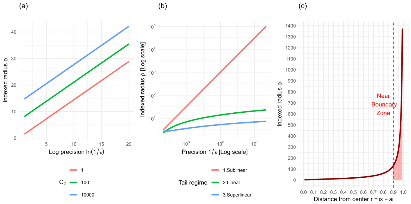
Figure 2.
Two-dimensional geometry of the sequential radii in the linear regime. The parameters are , , and . Panel (a) shows the indexed radius , illustrating the growth in the required number of terms as the point x approaches the boundary . Panel (b) shows the associated geometric radius , which records the reciprocal efficiency scale and decreases toward zero near the boundary and under increasingly strict precision demands.
Figure 2.
Two-dimensional geometry of the sequential radii in the linear regime. The parameters are , , and . Panel (a) shows the indexed radius , illustrating the growth in the required number of terms as the point x approaches the boundary . Panel (b) shows the associated geometric radius , which records the reciprocal efficiency scale and decreases toward zero near the boundary and under increasingly strict precision demands.
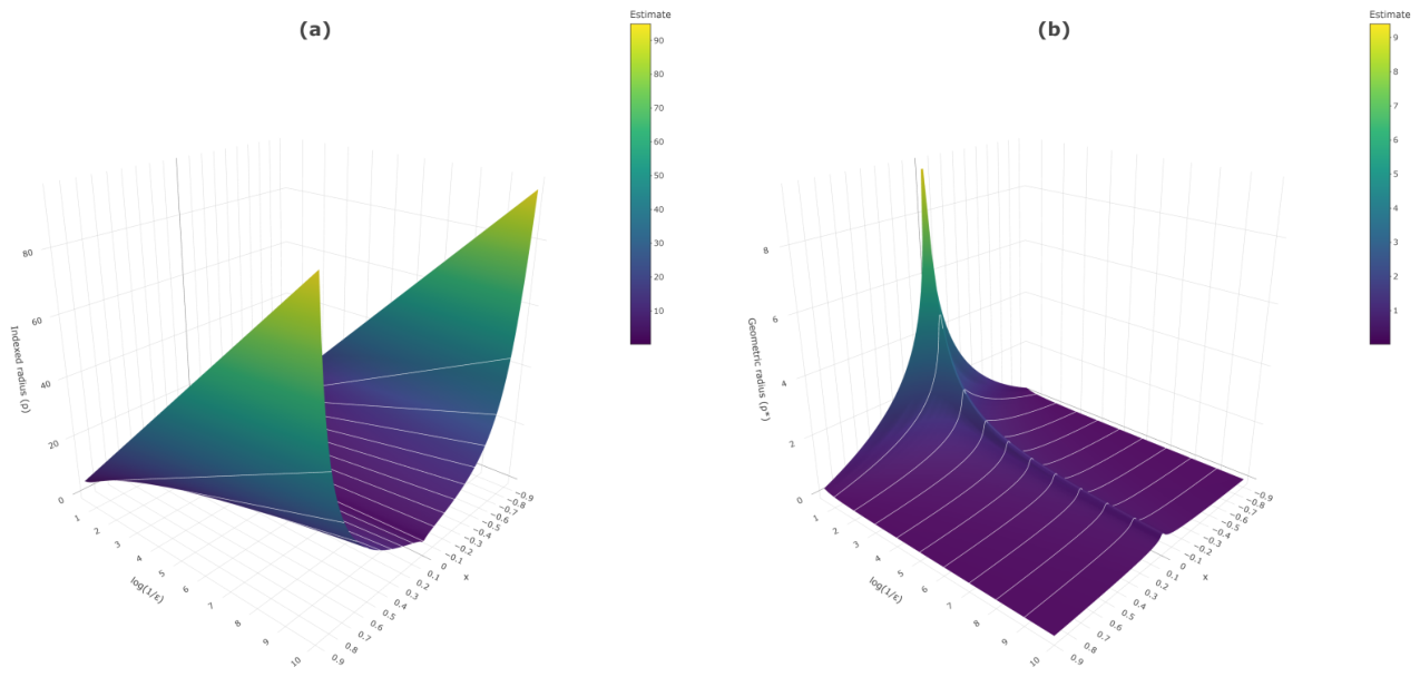
Figure 3.
The Venn diagram for the nested tail-regime subclasses inside the sequential-radius power-series classes for the space of Power series
Figure 3.
The Venn diagram for the nested tail-regime subclasses inside the sequential-radius power-series classes for the space of Power series
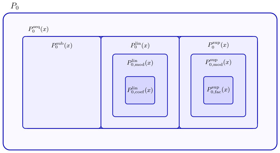
Table 1.
Classical radius ranges associated with the three tail-decay regimes for power series.
| Class | Tail regime | Typical tail | Classical Radius R | Position x |
|---|---|---|---|---|
| Class 1 | Sublinear | Usually | ||
| Class 2 | Linear | Usually | ||
| Class 3 | Superlinear | Any fixed |
Table 2.
Tail-decay regimes and the induced radii and .
| # | Tail regime | Tail asymptotic | Indexed-radius | Geometric radius |
|---|---|---|---|---|
| 1 | Sublinear | , | ||
| 2 | Linear | , | ||
| 3 | Superlinear | , |
Table 4.
Summary of catalog classical power series with linear/geometric/superlinear-type tails.
| Function(formula) | Series | Classic R | Indexed radius | Features |
| Function(formula) | Series | Classic R | Indexed radius | Features |
| Continued on next page | ||||
| Linear: Class 2 | ||||
| Lacunary geometric: | Lacunary geometric; nonzero exponents . | |||
| Reciprocal square: | Linear tail with algebraic factor N. | |||
| Logarithm: | Alternating geometric tail with algebraic factor . | |||
| Inverse hyperbolic tangent: | Odd lacunary logarithmic tail; coefficient factor . | |||
| Harmonic generating function: | Linear tail with logarithmic correction . | |||
| Legendre chi: , | Odd lacunary polylog-type tail; algebraic factor . | |||
| Arcsine: | Odd lacunary; central-binomial coefficient gives . | |||
| Binomial: , | Algebraic singularity at ; coefficient factor . | |||
| Polylogarithm: , | Linear tail with algebraic factor . | |||
| Catalan generating function: | Finite radius ; coefficient factor . | |||
| Lambert : | Finite radius ; Stirling gives . | |||
| Complete elliptic integral | Even lacunary; coefficient factor . | |||
| Secant: | Even lacunary; Euler-number asymptotic gives geometric factor . | |||
| Tangent: | Odd lacunary; Bernoulli-number asymptotic gives geometric factor . | |||
| Partition generating function: | Linear tail with subexponential correction . | |||
| Jacobi theta-type: | Square-lacunary; not directly Lemma 2; tail . | |||
| Superlinear: Class 3 | ||||
| Scaled exponential: | Full factorial; . | |||
| Sine: | Odd factorial subsequence; alternating; . | |||
| Cosine: | Even factorial subsequence; alternating; . | |||
| Sinh: | Odd factorial subsequence; positive signs; . | |||
| Cosh: | Even factorial subsequence; positive signs; . | |||
| Error: | Factorial with polynomial denominator; . | |||
| Bessel: | Squared factorial denominator; . | |||
Disclaimer/Publisher’s Note: The statements, opinions and data contained in all publications are solely those of the individual author(s) and contributor(s) and not of MDPI and/or the editor(s). MDPI and/or the editor(s) disclaim responsibility for any injury to people or property resulting from any ideas, methods, instructions or products referred to in the content. |
© 2026 by the authors. Licensee MDPI, Basel, Switzerland. This article is an open access article distributed under the terms and conditions of the Creative Commons Attribution (CC BY) license (http://creativecommons.org/licenses/by/4.0/).
Copyright: This open access article is published under a Creative Commons CC BY 4.0 license, which permit the free download, distribution, and reuse, provided that the author and preprint are cited in any reuse.