

Submitted:
01 June 2026
Posted:
02 June 2026
You are already at the latest version
Abstract
The multi-dimensional Elo rating system was designed to be a method of extending the more popular Elo system to model a wider variety of phenomena based on pairwise comparisons. This is useful in comparing the behaviours of machine learning models that would otherwise be black boxes. Unfortunately, the mElo rating system as it is currently formulated in the academic literature contains feedback loops that prevent the mElo rating system from correctly inferring an expected pairwise comparison matrix. In this paper, we propose an altered version of the mElo rating system that removes the feedback loops and ensures that a certain level of accuracy can be achieved. Furthermore, we demonstrate how the geometry associated with the model behind the multi-dimensional Elo rating system introduces complexities not present in the Elo rating system. We discuss some of these differences and how they affect the use and interpretation of the mElo rating system. We conclude the paper with a list of recommendations for the practitioner to ensure that the mElo rating system is being used correctly to infer a unique pairwise comparison matrix.
Keywords:
rating
; ranking
; matrix completion
; distributed algorithms
1. Introduction
The Elo rating system and its variants are very popular for comparing players in games (e.g., Chess), sports (e.g., FIFA), and e-sports (e.g., StarCraft) [1,2,3,4,5]. The results are useful for estimating the outcomes as well as other tasks such as match-making.
Most rating systems work by assuming that players’ skills can be quantified by a single number. As a result, the Elo rating system does not work well when the relation “is more likely to win against" is non-transitive. This is particularly important in the field of machine learning. Machine Learning (ML) results are often treated as black boxes, where the most effective way to assess whether one is better than another is to simply observe which one “wins" at a task. Hence, a system such as Elo that uses this type of binary input is invaluable. However, often ML solutions cannot be ranked using a total ordering [6,7].
The multi-dimensional Elo (mElo) rating system was first published in 2018 as a way of extending the Elo rating system to estimate probabilities of victory in the case where non-transitivity is present [6], in particular for ML applications. Unlike the Elo rating system, which gives every player a scalar-valued rating, the mElo rating system gives every player a vector-valued rating, and the probability of victory is given by a logistic function of a quadratic form between the two ratings. This rating system allows one to infer probabilities of victory in non-transitive settings.
The mElo rating system was designed to be a method of extending the more popular Elo system to situations where it would not normally work. This would, in theory, allow one to model a richer set of interactions. However, in practice, the mElo rating system routinely underperforms when compared to the Elo rating system [3,8,9]. We show here that the mElo rating system, as it is known in the academic literature, has not been used/implemented correctly; and we hypothesize that this fact is largely to blame for mElo’s underperformance.
The purpose of this paper is to answer the question: How does one know whether they are using the mElo rating system correctly? In this paper, we show that mElo rating system does work, but only if one is careful. In the original paper on the mElo rating system [6], there exists feedback loops which cause the mElo ratings to stop approximating the expected payoff matrix. Our paper bridges a gap in the existing literature by showing how the mElo rating system can avoid these feedback loops and how one can be certain that the mElo ratings are being used to estimate unique maximum likelihood estimators without getting stuck in local optima.
The underlying statistical model behind mElo maps vector-valued ratings to a matrix of probabilities of victory. This model has a greater level of expressive power than Elo. Unfortunately, that comes at a cost. The statistical model underpinning the mElo rating system is more complicated than the Bradley-Terry model used in Elo [10], and consequently, there are more ways that things can go wrong when using the mElo rating system. And the mElo rating system is not deterministic like the Elo rating system. This has the effect of making the results less amenable to interpretation.
In the original formulation of the mElo rating system [6], the update algorithm introduces the potential for feedback loops which can prevent the update algorithm from finding optimal mElo ratings. The intention of the mElo rating system is to find the optimum of a log-likelihood function. We use this understanding to present conditions on the data for this optimisation problem to have a unique solution modulo symmetry, which assures us that the rating system works correctly.
This paper also looks at situations in which it appears that the mElo rating system is not working when in fact it is. We show that there are multiple sets of mElo ratings that correspond to the same set of probabilities of victory, arising from the symmetry group associated with the optima. This can make it difficult to interpret mElo ratings. We argue that this is does not mean that the mElo rating system is flawed, even if experiments may not appear reproducible.
The aim of this paper is to be useful to the statistician or data scientist who may be considering using the mElo rating system. Additionally, we hope the paper is of interest to those who are work in the design and analysis of algorithms and would appreciate a specific case study.
In summary, the contributions of this paper are.
- 1.
- We refine the mElo algorithm from [6] to eliminate the problem of feedback and to be more robust.
- 2.
- We discuss necessary and sufficient conditions to determine whether probabilities of victory can be uniquely determined from a given dataset.
- 3.
- We explain why the mElo rating system will not find a maximum likelihood if all players begin with the same rating.
- 4.
- We consider the identifiability problem associated with the mElo rating system. We show that that there are different sets of ratings that correspond to the same set of probabilities. We discuss the implications this has for interpreting mElo ratings, and explain that while it has its inconveniences, this ambiguity in mElo ratings is actually a good thing.
- 5.
- We verify these theoretical results using numerical experiments.
- 6.
- Finally, we conclude with a checklist for the practitioner, to allow a data scientist to use the mElo rating system correctly.
2. Background
The multi-dimensional Elo (mElo) rating system [6] is an extension of the better known Elo rating system [1]. The main difference between mElo and Elo is that mElo can be used to estimate probabilities of victory when the binary relation “is more likely to win against" is non-transitive. That is we have situations where there exist three players A, B, and C where Player A is more likely to win against Player B, who is more likely to win against Player C, who in turn, is more likely to win against Player A.
In this section, we introduce the mElo rating system. In Section 7.2, we provide a numerical simulation on a test problem.
Both the Elo and mElo rating systems assume that the probabilities of victory can be given according to an expected payoff matrix P, where
Because both Elo and mElo are used for modelling zero-sum games without draws1, we have the requirement
The goal of both the Elo and mElo rating systems is to estimate this expected payoff matrix based on a dataset consisting of an order list of the outcomes of multiple games.
Neither the Elo nor mElo rating systems work directly with the expected payoff matrix, instead both systems work with an advantage matrix A, where the advantage matrix is related to the expected payoff matrix by
where is the logistic function2. The zero-sum nature of the game implies that A is skew-symmetric, i.e., .
The Elo rating system implicitly assumes that the advantage matrix is a strongly transitive additive comparison matrix (STACM) [6,11]. A STACM is a matrix M where for all unique triples , . One important feature of STACMs is that they can be expressed by finding a rating for every player, such that the advantage matrix’s entries are given by . In the context of Elo, these numbers are called Elo ratings and the Elo rating system works by estimating these Elo ratings (up to addition of a constant) using stochastic gradient descent [8].
The set of STACMs form a strict subset of rank-2 skew-symmetric matrices. The space of skew-symmetric matrices orthogonal to the space of STACMs are called cyclic matrices. The mElo rating system is able to model more complicated relationships by assuming that the advantage matrix is skew-symmetric matrix of fixed rank that contains a non-trivial cyclic component. The mElo rating system contains a hyper-parameter k, where it assumes that the advantage matrix is of rank (skew-symmetric matrices must be of even rank).
Let be the set of skew-symmetric matrices of rank at most . The types of advantage matrices inferred by the Elo rating system and the mElo rating system, for different values of k are shown below.
The mElo rating system calculates probabilities of victory by assigning every player a dimensional vector called their mElo rating. The advantage matrix is given by
where is a matrix who’s columns are the mElo ratings of each player and , is the block diagonal matrix whose blocks are given by
Therefore, given two players i and j, with mElo ratings and , the mElo rating system predicts that Player i will win against Player j with probability
The Elo and mElo rating system both include a method of updating the ratings of two players based on the outcome of a game between them. Let us consider a game between players i and j. If Player i wins the game, then we assign and , and if j wins, then and , and the (un-normalised) update rule for the players’ mElo ratings takes the form
for Player i, and
for Player j, where
- is the mElo rating of Player i at game t.
- is the learning rate.
This update formula can be derived by differentiating the log-likelihood function associated with a single game.
with respect to the entries of C. That is, the mElo ratings are updated after each game using stochastic gradient descent on the log-likelihood function.
A key advantage of both the Elo system and mElo system (as described above) is that update rules affect only the ratings of the player involved in the game. And likewise predictions about outcomes can be made using only the ratings of the players concerned. We refer to this as the distributed property of a ratings system, and it is very useful, particularly when the pool of players is large.
To summarise, the mElo2k rating system consists of
- A pair of hyper-parameters k and , where is the learning rate.
- An expected payoff matrix of rank .
- An expected payoff matrix given by .
- A vector of parameters for each player i.
- A formula for updating ratings after the completion of each game.
2.1. Original Formulation of the mElo Rating System
Readers of [6] may notice that our rating system differs slightly from the mElo rating system presented there. In this subsection, we explain how our formulation of the mElo rating system differs from theirs and why. In the original mElo rating system, the authors also model the advantage matrix as a rank- skew-symmetric matrix, but the authors also assign each player an Elo rating in addition to a vector-valued rating. After each game, both the Elo ratings and the vector-valued ratings are updated using stochastic gradient descent. Expressed mathematically, this version of the mElo rating system assigns every player a rating , where , and . The probability of victory is calculated by
and ratings are updated according to
and
where and are separate learning rates. The idea behind this choice was to separate the inference of the cyclic component from the transitive Elo ratings.
In our paper, we will not focus on the scalar component of the mElo rating system. We do this for two reasons. First, we believe this formulation to be misleading. It is not true that the cyclic and transitive components are truly separated. There is no mechanism in place that ensures that is a cyclic matrix. In practice, the component of the advantage matrix given by C can also contain a large transitive component.
Second, we omit the scalar component r in order to simplify the analysis in subsequent sections of this paper. The results presented are not affected by the presence of a scalar component and will hold in the original formulation of [6], although it would be harder to see what is happening.
3. Feedback Loops
One crucial difference between the Elo and mElo rating systems is that the lengths of the gradient vectors in the likelihood function are bounded in Elo and unbounded in mElo. Both systems attempt to find maximum likelihood estimators by applying stochastic gradient descent to their respective log-likelihood functions. However, since the gradients in the mElo rating system can be of any size, the estimated parameters can change by huge amounts after even a single game. These huge steps can lead to feedback cycles in which our parameter estimates either grow incredibly large and miss the optima of the log-likelihood function. Or the parameter estimates can negatively interfere with each other, shrink towards the origin and also, miss the optima of the log-likelihood function. Fortunately, these feedback problems can be mitigated by normalising the parameter updates with each game.
In this section of the paper, we demonstrate the problems of positive and negative feedback on a toy problem involving two players, (and hence a rank-2 advantage matrix) and a learning rate . We show how the learning rate of the mElo update algorithm can lead to the players’ mElo ratings shrinking towards the origin at an exponential rate.
Let us say we have two players called y and z. Initially, we assign these players the rating vectors
After players y and z play a game, their ratings are updated according to
Since, and , we can simplify the above expressions and show that.
We are going to look at what happens when is small and . We will look at when it is possible for x to move away from the origin and when x will be pulled back to the origin.
When the term will always lie in the interval . Now, , so regardless of the outcome of the game, we always multiply by a positive number. This means that regardless of the outcomes of the games, the sign of will never change. Hence, the odds given by the mElo rating system will be in the following intervals
- , if x starts with a negative value.
- , if x starts with a positive value.
- , if x starts at zero, i.e.,, .
Without loss of generality, we presume that x begins with a positive value. If Player z wins, we multiply x by , and if Player y, then we multiply x by . Assuming that x is close to zero, and after N games, we would expect Player y to win of these games and lose games, where p is the true probability that Player y wins against Player z. Over the course of N games, for small values of x, the value of x after these games can be approximated
As the number of games N approaches infinity, x will increase exponentially, decrease exponentially or do neither if is greater than one, less than one, and equal to one, respectively.
This shows that if the probability p that i beats j satisfies the inequality
Then x will tend to shrink towards the origin at an exponential rate. As was mentioned before, if , then, regardless of the outcomes of the games, the mElo rating vectors will never predict that i will win the game with probability .
From Equation (3) we see that for values of , there exist values of p such that if i beats j with probability p, then and will still shrink towards the origin at an exponential rate. This means that the mElo ratings will not approximate the expected payoff matrix, which is a key purpose of the mElo rating system. For a more in-depth discussion and examples where the mElo ratings grow without bound instead of shrinking, the reader is invited to consult [12].
3.1. Normalised Updates
These feedback loops occur because in the mElo rating system, the difference between and can grow without bound. We recommend avoiding these feedback loops by normalising our updates, i.e.,after a game between Players i and j, the mElo2k ratings vectors are updated according to the formulae:
and
where
This means that the mElo update algorithm still explores the space of -sized matrices C, but does so in only in steps whose size has upper and lower bounds.
3.2. Numerical Simulations
To illustrate the results, we run an experiment in which we have two players: y and z. Player y begins with a mElo rating of and Player z begins with a mElo rating of . In this experiment, we have two players with perpendicular mElo ratings of equal length. When we set the learning rate to be , and the probability of y beating z is equal to , then Inequality Equation (3) is satisfied, and we would expect to see exponential shrinkage. We can see that the lengths of both players’ mElo ratings do, in fact, shrink at an exponential rate. A diagram of this experiment is shown in Figure 1.
This is a single specific case of feedback loops in the mElo rating system. If the learning rate is too large, then the mElo rating vectors will increase exponentially rather than decrease. In situations where there are more than two players, an un-normalised mElo rating system can avoid these feedback loops when the learning rate is low. The reader is encouraged to read [12] for more information. The fact that we can show that it does break down in certain edge cases is representative of a larger problem with the mElo rating system and motivates the need for normalised updates.
4. Initialising mElo Ratings
The standard Elo rating system is an iterative algorithm and thus requires initialisation, but it may be initialised by giving every player the same rating. This is appealing as it treats the players equally and can be simply implemented. It also allows for easy, incremental addition of players (for instance, as new players join a game like Chess).
It seems to have been assumed that the mElo rating could be similarly intitialised3, but it cannot. In this section, we show that if we assign every player the same mElo rating, then the set of players’ mElo ratings will be stuck in a local, stationary point, and will not be able to find a maximum likelihood estimator for C. We then give necessary and sufficient conditions to initialise the mElo rating vectors such that the mElo ratings will approach a maximum likelihood estimator with probability one.
The mElo rating system assumes that the advantage matrix is of rank . The ratings are updated using Equation (2), i.e.,
where the matrix is a block diagonal matrix made up of copies of
If we consider the th and th entries of player i’s mElo rating, , then the direction in which we update this vector is
Each 2-dimensional component of a player i’s mElo rating is updated in the direction of player j’s corresponding 2-dimensional component multiplied by . The only effect the other components of have on is through the term . This leads to the following theorem.
Theorem 1.
Consider a matrix C of mElo ratings. If the column space of is spanned by the vectors , then the column space of will be spanned by the vectors with probability one for all sufficiently large values of time step t (presuming all players can play one another).
Proof.
Let C be a matrix of mElo ratings with columns spanned by , with each iteration of the update algorithm. We take two players i and j and add a scalar multiple of to , and some scalar multiple of to . This means that after a large number of iterations, each player’s mElo rating will be given by some linear combination of , for . Since , the columns of C will all be made up of linear combinations of and , for all values of . Thus, the space is spanned by the vectors . □
Notice how in Theorem 1, the rank of C almost surely changes from
to , and does not increase past that value.
A corollary of this fact is that if we initialise every player with the same mElo rating c, then the matrix will have a column space that will always be spanned by c and and thus never be larger than rank 2. That is, the matrix cannot express any of the mElo ratings outside of this very limited subset.
This means that the only way we can approximate a maximum likelihood estimator for a rank advantage matrix is if we initialise C with full rank or with a column space X such that spans .
If we assign players’ initial mElo ratings with random values drawn from a continuous distribution, the initial matrix C will be of full rank with probability one.
This by itself is a rather loose set of conditions on randomly initialising the mElo ratings. The condition is just that we sample our matrix C from a continuous distribution over a subset of with positive measure. In the interests of making the mElo rating system fair and simple to implement, we suggest initialising the mElo ratings independently. This treats each player equally, and eliminates the need for any extra coordination between the population of players.
The result is a very simple initialisation, but it has one inconvenient consequence. Since we are initialising ratings randomly, we no longer have a deterministic rating system. However, pseudo-random numbers (PRNs) provide a means to specify a reproducible rating system if specify details such as PRN seeds and the exact method of generation.
5. Symmetries and Non-Unique Ratings
One of the main sources of complication in the mElo rating system is that it has a significantly more complex symmetry group than the Elo rating system.
In the Elo rating system, if we add a constant to every player’s Elo rating, then the underlying advantage matrix does not change, i.e., it is invariant under shifts. Usually, there is an additional criterion added to an Elo-like system to create a unique solution: for instance, it is common to require that the mean rating is a fixed value (such as zero). This removes the translational symmetry, resulting in unique solutions.
The symmetry of the mElo rating system is the group4 of transformations on the matrix C that leave the advantage matrix unchanged. That is, the group of transformations g on the matrix of ratings C such that . This symmetry group is well-known in mathematics [13]. It is the symplectic group, defined by exactly this transformational invariance.
The fact that mElo has a more complicated symmetry group means that one cannot alter the mElo rating system to obtain an algorithm that estimates a unique, maximum likelihood estimator for C with the distributed property.
The distributed property of the Elo or mElo rating system means that the results of a game between Players i and j only affect the ratings of Players i and j. The distributed property implies that Player w’s rating won’t change as a result of a game between players x and y. It is this distributed property that makes it possible to scale an algorithm like mElo to a massive population size. Every player is given their own ratings along with identical instructions on how to update it. There is no need for a single entity to keep track of each player. The system can therefore be distributed across a set of administrators, each keeping track of their own subset of players.
Uniqueness (of ratings) isn’t just a convenience or a means towards reproducible experiments. If there were a unique matrix of ratings C corresponding to every advantage matrix A, then this would allow one to assign meaning to each of the ratings, which would in turn allow us to interpret the mElo ratings. For instance, one’s Elo rating in Chess is used to assign Grand Master status (at a rating above 2500).
Unfortunately, in mElo, unique ratings don’t exist without sacrificing the distributed property. The proof can be found in the final chapter of [12]. It is quite technical, so we omit it here. However, we can understand the gist of it if we consider that the rotational subgroup of the symplectic group commutes with the update process of the mElo rating system. This means, that the mElo rating system will behave exactly the same if we rotated all the mElo ratings by a given amount. However, that would change all of the ratings, not just those of the primary players. Hence, any transformation designed to force a unique orientation onto the set of ratings (e.g., a transformation to ensure the mean direction was fixed in the same manner that Elo ensures the mean rating value is fixed) would necessarily change all of the ratings after each update.
It is a major difficulty to lose the distributed property, so in all implementations of mElo of which we are aware, uniqueness is sacrificed. This makes the mElo rating system harder to use when it comes to interpreting results, as the values of a single mElo rating vector will tell us very little. Only the relative orientations of ratings vectors has meaning.
One important takeaway from this section is that if two statisticians were to independently run the mElo rating system (with random initialisations) and fit mElo ratings to the same sets of players and game outcomes, then, with high probability, the resulting set of mElo rating vectors would differ. Likewise, if the same sets of players were to play in two tournaments, then ratings derived separately for the two tournaments would differ (because there would likely be different outcomes in some matches). But this is OK. It is not an indication that either statistician had made a mistake or that the system is misbehaving.
If one wishes to assess the accuracy of mElo, then one must assess the accuracy of the advantage matrices, not the ratings themselves.
6. Symmetries and Non-Unique Ratings
One of the main sources of complication in the mElo rating system is that it has a significantly more complex symmetry group than the Elo rating system.
In the Elo rating system, if we add a constant to every player’s Elo rating, then the underlying advantage matrix does not change, i.e., it is invariant under shifts. Usually, there is an additional criterion added to an Elo-like system to create a unique solution: for instance, it is common to require that the mean rating is a fixed value (such as zero). This removes the translational symmetry, resulting in unique solutions.
The symmetry of the mElo rating system is the group5 of transformations on the matrix C that leave the advantage matrix unchanged. That is, the group of transformations g on the matrix of ratings C such that . This symmetry group is well-known in mathematics [13]. It is the symplectic group, defined by exactly this transformational invariance.
The fact that mElo has a more complicated symmetry group means that one cannot alter the mElo rating system to obtain an algorithm that estimates a unique, maximum likelihood estimator for C with the distributed property.
The distributed property of the Elo or mElo rating system means that the results of a game between Players i and j only affect the ratings of Players i and j. The distributed property implies that Player w’s rating won’t change as a result of a game between players x and y. It is this distributed property that makes it possible to scale an algorithm like mElo to a massive population size. Every player is given their own ratings along with identical instructions on how to update it. There is no need for a single entity to keep track of each player. The system can therefore be distributed across a set of administrators, each keeping track of their own subset of players.
Uniqueness (of ratings) isn’t just a convenience or a means towards reproducible experiments. If there were a unique matrix of ratings C corresponding to every advantage matrix A, then this would allow one to assign meaning to each of the ratings, which would in turn allow us to interpret the mElo ratings. For instance, one’s Elo rating in Chess is used to assign Grand Master status (at a rating above 2500).
Unfortunately, in mElo, unique ratings don’t exist without sacrificing the distributed property. The proof can be found in the final chapter of [12]. It is quite technical, so we omit it here. However, we can understand the gist of it if we consider that the rotational subgroup of the symplectic group commutes with the update process of the mElo rating system. This means, that the mElo rating system will behave exactly the same if we rotated all the mElo ratings by a given amount. However, that would change all of the ratings, not just those of the primary players. Hence, any transformation designed to force a unique orientation onto the set of ratings (e.g., a transformation to ensure the mean direction was fixed in the same manner that Elo ensures the mean rating value is fixed) would necessarily change all of the ratings after each update.
It is a major difficulty to lose the distributed property, so in all implementations of mElo of which we are aware, uniqueness is sacrificed. This makes the mElo rating system harder to use when it comes to interpreting results, as the values of a single mElo rating vector will tell us very little. Only the relative orientations of ratings vectors has meaning.
One important takeaway from this section is that if two statisticians were to independently run the mElo rating system (with random initialisations) and fit mElo ratings to the same sets of players and game outcomes, then, with high probability, the resulting set of mElo rating vectors would differ. Likewise, if the same sets of players were to play in two tournaments, then ratings derived separately for the two tournaments would differ (because there would likely be different outcomes in some matches). But this is OK. It is not an indication that either statistician had made a mistake or that the system is misbehaving.
If one wishes to assess the accuracy of mElo, then one must assess the accuracy of the advantage matrices, not the ratings themselves.
7. Uniquely Recovering the Advantage Matrix
Another way to view the mElo rating system is through the lens of low-rank matrix completion. The purpose of the mElo ratings is to be able to infer the entries of a low-rank matrix (the advantage matrix) using a smaller number of observed entries (the outcomes of games between players) [14]. In this section, we review the matrix completion problem, show that mElo is a particular example of low-rank matrix completion, and use this fact to derive necessary and sufficient conditions for an advantage matrix to be uniquely recovered.
Matrix completion problems typically involve finding the entries of an unknown matrix , given some observed entries . Without additional assumptions, this problem is impossible, so we assume that the matrix has some underlying structure. In this case, we presume that M has a fixed rank . This assumption makes it possible to calculate the entries of M based on other entries under some conditions.
It is possible that the observed entries of the low-rank matrix M have also been corrupted by noise. In that case, the goal then becomes to find some rank-r matrix , that minimises a distance function between the observed partial matrix, and the completed low-rank matrix [14].
In the mElo rating system, we are attempting to infer the advantage matrix A, which is both rank- and skew-symmetric (because the observed entries of the matrix are the outcomes of games with a winner and loser). The mElo rating system completes the matrix under noise by finding an advantage matrix , that maximises the log-likelihood function
where D is the ordered list of pairs of players who play each another and is the indicator variable that equals one when Player i beats Player j, i.e., . In most settings, only a subset of players will compete directly, and so the mElo rating system can be naturally viewed as an example of a matrix completion problem.
In deriving necessary and sufficient conditions for the advantage matrix to be uniquely completable, we take the necessary and sufficient conditions for generic matrix completion derived in [15,16] and adapt them to our purposes, which differ somewhat from typical matrix completion problems because of the addition of properties such as skew symmetry.
Definition 1.
We say that Player i is comparable to a set of players Γ if there is a bounded maximum likelihood estimator for Player i’s mElo rating given fixed mElo ratings for every player in Γ.
Theorem 2.
Take a set Γ of players and Player . Let be the set of mElo ratings of the players in Γ, and let players be the set of players in Γ that play against Player i and win, and let , be their respective mElo ratings. Let
be the set of players in Γ that play against Player i and lose, and let , be their respective mElo ratings. Then Player i is comparable with the set Γ if and only if is contained in the convex cone of the mElo vectors , , .
- Remark: Note that the players in can play against Player i multiple times, and therefore the sets and need not be disjoint.
Proof.
A mathematically precise definition of Player i being comparable to the players in is that the following log-likelihood function given below has a unique local maximum.
where is the player in that plays player i at time step t and is the indicator variable that is equal to 1 if Player defeats Player i at time step t and is equal to zero otherwise.
Since the is a binary variable, each term in the summand in will either be if Player i wins or if Player j wins. These functions are all concave down and bounded from above but not bounded below. If Player i beats Player and we move x in the direction , then the corresponding term in will increase and if we move x in any direction perpendicular to , the corresponding term in will not change value. Similarly if Player i loses against Player , then moving x in the direction will increase the corresponding term in , but would not change if we moved x in any direction parallel to .
Since each summand in is a concave down function, the function is concave down as well. Since each summand is bounded from above but not from below, and there are a finite number of summands, is also bounded from above.
If there exists a line v such that we can take all of the vectors
, project them onto v, and have the projection be positive then that means that if we move x along this line v, then will increase indefinitely. If no such line v exists, then no matter which direction we move x in, if we go far enough, one of the summands, will decrease indefinitely, and will approach .
Since is concave down, and if , , then must have a unique local maximum and Player i is therefore comparable to the players in . This is true if and only we cannot construct a line v.
The statement, there does not exist a v such that
all have positive projections onto v is equivalent to the statement that is contained in the convex cone of the vectors
. Therefore, Player i is comparable to if and only if is contained in the convex cone of the vectors .
So to summarise, if is contained in the convex cone of the vectors , then that means if we move x in any direction sufficiently far away from the origin, then will approach . Thus has a unique local maximum and i is comparable to . This proves one direction of Theorem 2.
If is not contained in the convex cone of the vectors
, then there exists some direction v such that all the vectors
have positive projections onto v and if we move x along the line v, then is an increasing function of . This proves Theorem 2 in the other direction. □
The intuition behind this theorem is that with every game between Player i and a member of , Player i receives some information about the direction in which to move their mElo rating in order to increase their log-likelihood value. Once Player i plays enough games with enough members of , they get enough directions such that these directions begin to cancel one another out. And when all these directions have cancelled one another out we have arrived at a maximum likelihood estimator for , given .
If we have a population of m players and we introduce a new player. This new player’s mElo rating introduces new variables into the optimisation problem and thus we are optimising the log-likelihood function over a space with dimensions. Due to the symplectic symmetry of the log-likelihood function, we can remove dimensions from the domain of the objective function (noting that usually ). Whenever a player is comparable to the existing network, we have information about how far we should move in each of the new dimensions. This means that the log-likelihood function will have local maxima in the directions corresponding to the new dimensions.
Another way we can think about the problem is that we could resample the data and bootstrap the mElo updates updating our mElo ratings using stochastic gradient descent. In the case that a player was not comparable, their mElo ratings would diverge to positive infinity because there would be at least one direction in which we could not update our mElo rating.
This brings us to the main difference between matrix completion in [15], and the mElo rating system. In the typical matrix completion problem, we just need to know the combinatorial properties of the mask (i.e., who plays who). In the mElo rating system, we have a directed interaction network, where people often only play other players once and never again. If it were the case that for every pair of players, we observed enough games between so that we observe both players win at least one game each, then our problem would reduce to that of [15].
Let M be the total population of all the players. A necessary condition for the advantage matrix to have a unique maximum likelihood estimator, is for every player i in the population to be comparable with the set . This follows from Theorem 1. If a player in the population was not comparable to the other players in the population, then there would not be a unique maximum likelihood estimator for , given mElo ratings for all players , and hence there would not be a unique advantage matrix A.
We now prove that this condition is necessary but not sufficient. Use the cycle graph and the mElo rating system with 2-dimensional mElo rating vectors () as an example. Imagine, we have a population of four players indexed by A,B,C and D, where Player A cannot directly play D and Player B cannot directly play C. We can demonstrate that the probability that A beats D is under-determined. We provide a visual proof in the diagram in Figure 2. From our proof of Theorem 2, if we know the probability that Player i beats Player j, then we know ’s component in the direction but not in any other direction.
7.1. Sufficient Condition
Now that we have presented a necessary condition for the advantage matrix A to have a unique maximum likelihood estimator, we present a separate condition that is sufficient. From this sufficient condition, we are able to create a polynomial-time algorithm that can check whether the data set corresponds to a unique maximum likelihood estimator for A.
Here, we adapt the matrix completability algorithm from [15] to suit our purposes. The algorithm takes as input, the interaction network for the players in the population. This is a directed graph, where the nodes are the players and there is a directed edge from Player i to Player j if Player i has beaten Player j at least once.
The algorithm works by taking a minimal sub-population of the players such that the advantage matrix associated with this sub-population is uniquely defined. If it is the case that we can observe a clique of players, and we have estimates of the probabilities of victory between all pairs of these players, then the advantage matrix (i.e., the maximum of the log-likelihood function) associated with these players is uniquely defined. We assign mElo ratings to these players so as to maximise the log-likelihood function.
The algorithm works by iterating through all the players that do not yet have unique mElo ratings. If the algorithm finds a player that is comparable to the players who have been assigned mElo ratings, we then add the player to the population, and recalculate the mElo ratings to maximise this new log-likelihood function. The algorithm then searches for another player that is comparable to this new group, and repeats this process of assigning mElo ratings. If the algorithm cannot, at any stage, find a player that is comparable to its current set of comparable players, then it returns a value of null.
Our algorithm is based on a sufficient condition that may or may not be a necessary condition. It is still an open problem to determine whether there are any datasets that have a unique maximum likelihood estimator but would be assigned a null value by our algorithm. The algorithm is described in pseudocode in Algorithm 1.
| Algorithm 1 An to determine whether there exists a unique maximum likelihood estimator for P. |
|
7.2. An Example
In the previous section, we established conditions for a player to be comparable to the other players in a population. Here, we demonstrate this idea using numerical simulation on a toy problem where we have three players P1,P2, and P3. They are given the following initial mElo ratings.
We introduce a new player called and consider four scenarios in which wins and loses against the other players. In each of the four scenarios, we plot the relevant vectors used to determine whether is comparable to the set of other players. The scenarios are
- Scenario 1: wins against and . The log-likelihood function increases in the direction and . The log-likelihood will increase in any direction given by a convex combination of these two vectors. Therefore, in this scenario, there is no unique local maximum for , given and .
- Scenario 2: wins and loses against . Because only plays , the log-likelihood function only changes in the direction , but this time but the function does not keep increasing as one moves further along . The information in this game is enough for one to determine the component of perpendicular to , but not any of the other components.
- Scenario 3: wins against , , and . In this case we have a log-likelihood function similar to that of Scenario 1. Because is contained in the convex cone of and , the fact that we have observed winning against , does not give us very much new information and is not enough to make comparable to , , and .
- Scenario 4: wins against , , and but also loses against . In this scenario the convex cone of the vectors , , , and contains . We can see that the log-likelihood function corresponding to this scenario has a single, unique local maximum. In this case, a maximum likelihood estimator for is uniquely determined from the available data.
The four scenarios are illustrated in Figure 3, which shows the log-likelihood functions. We can see that only Scenario 4 has a well-defined minima showing that in only that case is comparable to the set .
8. Simulation Example
In this section, we will consider a toy problem of three players with three players, called Players , , and , with mElo ratings , , , respectively. It differs from the previous case in that we start with a known expected win/loss matrix between these players:
These three players are given the following (notionally randomised) initial mElo ratings.
These ratings correspond to an expected payoff matrix of
Note that this quite a long way from the true matrix.
We now show how one can update the mElo ratings after game outcomes to better approximate P.
At each iteration of our simulation, we pick two players randomly from our population. For example, we start by picking Players 2 and 3. The true probability that Player 2 beats Player 3 is equal to . In our simulation, we have Player 2 win against Player 3 (even though it was unlikely).
We update the mElo ratings of players 2 and 3 according to equations Equation (4), and Equation (5) respectively, as follows (taking our learning rate )
- i = 2, j = 3;
- = 1, (Player i beat Player j);
- t = 0, (we are updating our initial ratings);
- ;
- (from our initial ratings); and
- (from our previous calculation of ).
Substituting our values into Equation (4), we obtain the update
Similarly, we can use Equation (5) to update Player 3’s mElo rating
Since Player 1 did not play against anybody in the first timestep, we have .
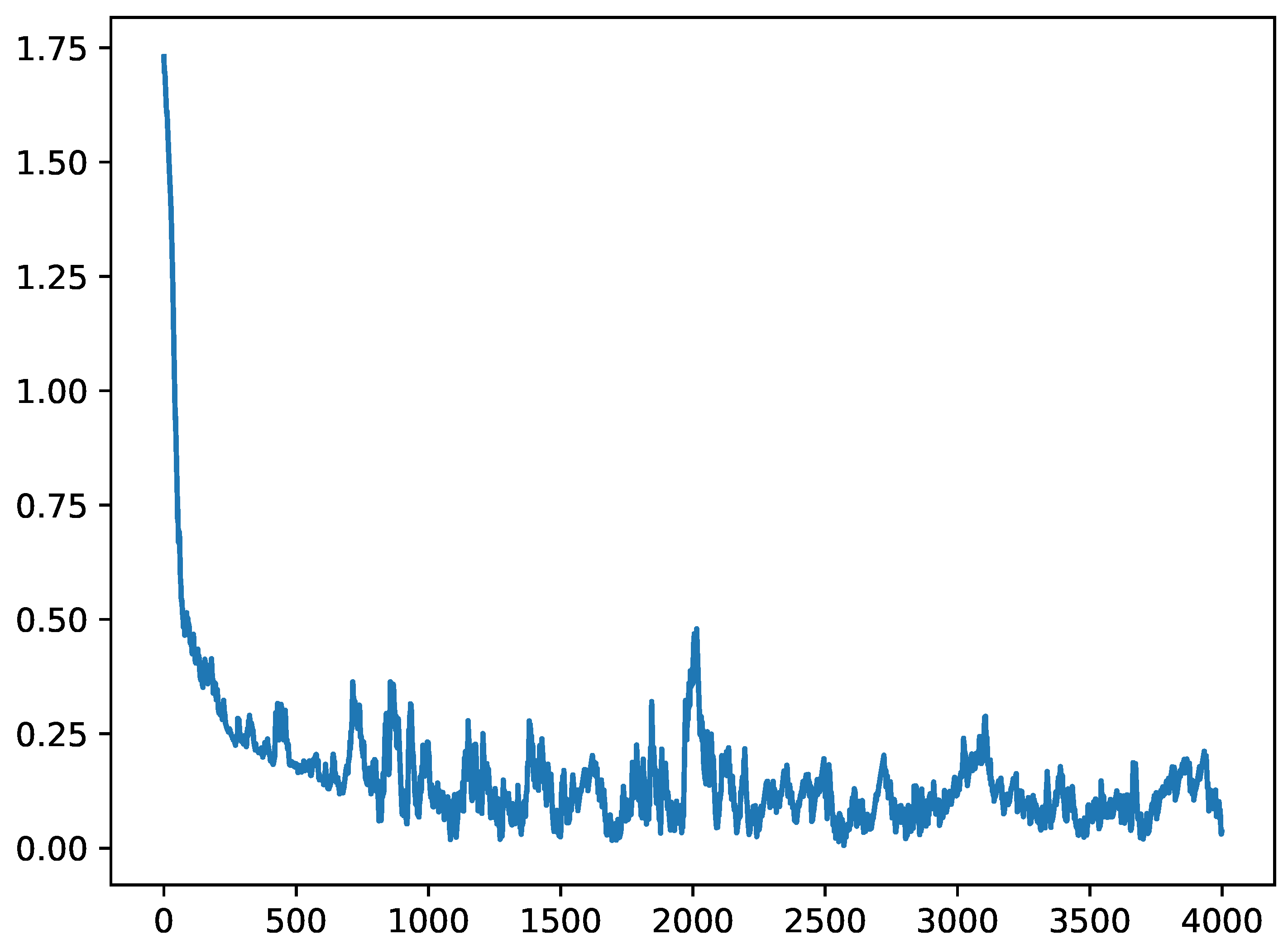
We continue our simulation for a total of 4000 games. At each timestep, we select two players i and j uniformly at random, have Player i beat Player j with probability given by , and update the player’s mElo ratings using equations Equation (4) and Equation (5). The results of our simulation are shown in Figure 4.
In Figure 4, we show the changes in mElo ratings for all 3 players. The first and second components of each player’s mElo rating vector is shown on the horizontal and vertical axis respectively. The change of each player’s mElo ratings are shown as three continuous lines on the plane. We can see the one visible endpoint of each line corresponds to each of the players’ initial mElo ratings, the arrows represent the values of the players’ mElo ratings at the end of the simulation.
In Figure 5, we show the Frobenius distance between the approximate expected payoff matrix and the true expected payoff matrix P. We can see that the mElo rating system is indeed approximating the true expected payoff matrix as required. We can also see that after approximately 1000 iterations, the mElo ratings stop improving. After this point, the mElo ratings just move around a set of mElo ratings that correspond to the true expected payoff matrix, because the step sizes after each iteration are bounded from above and below within a neighbourhood of the true values, the mElo rating system cannot obtain more precise results. Hence, the noisy estimates of P.
If we had used a learning rate less than , then it would take more iterations for the mElo ratings to find an approximation to P, but the approximation of P would be more precise. There is an inherent trade-off when selecting a learning rate for the mElo rating system. A smaller value of leads to more precise estimates but slower convergence, and a larger value of leads to faster convergence but less precise estimates. The optimal selection of is an important problem, especially in situations where the true expected payoff matrix changes over time, and there is limited data available.
However, the variations can actually be a desirable property in the analysis of games because players’ abilities in a sport (for instance) vary over time, and hence an iterative algorithm needs to adapt its estimates. Some noise is inevitable. In ML applications, we might wish to use mElo with a reducing learning rate schedule (much as is used in many other optimisation contexts, such as the temperature schedule used in simulated annealing) in order to converge to fixed estimates within some time threshold.
In our simulation, we ensure that all three players can play one another an unlimited number of times. This ensures that the games scheduled satisfy the properties in Section 6 and the expected payoff matrix estimated in this process is unique.
Even though the expected payoff matrix obtained was unique, the matrix C of mElo ratings was not. Since we randomly, initialised our ratings at , , and , we obtained a matrix of mElo ratings
If we had started with the same mElo ratings but rotated degrees anti-clockwise, then we would end up with a matrix C in which the columns were also rotated degrees anti-clockwise. It is important to remember that both C matrices would be equally correct.
9. Advice to the Practitioner
This section summarises the results from this paper as a guide to the practitioner, where we provide a few instructions to the practitioner so they can be more sure that they are using the mElo rating system correctly.
When using the mElo rating system, we recommend that the practitioner does the following:
- Before fitting mElo ratings to the data use the list of games to determine which players are comparable with which other sets of players, using the sufficient condition given in Section 7. Only proceed if the condition is satisfied.
- When initialising the mElo ratings of each player, make sure they are initialised in such a way that the matrix C of ratings is of full rank. This can be done by randomly assigning players their initial ratings. If the initial ratings are sampled from a continuous probability distribution, then C will be of full rank with probability one.
- When updating mElo ratings, make sure to use the normalised version of the mElo update algorithm to ensure that the ratings stay robust.
- When assessing results (for instance from simulations), do not expect ratings vectors to match a preassigned set of “ground-truth" vectors. Assess the accuracy of the advantage or probability matrices.
10. Conclusions and Future Work
We hope that the results presented here will help the data science and ML communities use the mElo rating system correctly, when it is applicable. Further details of the mElo rating system can be found in [12]. Despite the limitations documented here, the mElo system allows the analysis of game outcomes (and ML comparisons) in a much richer manner than simple Elo, and it shows much promise.
Moreover, we suspect that the desire for such richness will lead many future authors to reach for systems that extend Elo into more complex vector spaces, and hence developing our theoretical understanding of such systems is important. The properties described here revolve around the specific mElo proposal, but the underlying understanding of how symmetries affect a rating system is applicable to almost any such system.
In the future, we aim to extend this understanding in several ways. Both the Elo and mElo rating systems are related to particle filters and Hidden Markov Models in that they are designed to track the movements of a partially observed stochastic system (here an expected payoff matrix) that is continuously changing over time. The time series aspect of the mElo rating system has not yet received much study. If the sampling rate multiplied by the learning rate is less than the speed at which the true parameter values are moving, then we hypothesise that the rating system will not work. In the future, we intend to derive mathematical conditions under which one can detect this phenomenon and know that the mElo rating system is applicable.
In addition, because mElo has a larger parameter space than Elo, it will require more data to converge to an optimum. In future work, we intend to place realistic bounds on how much data of each type is required to establish a certain level of confidence in the results of the mElo rating system for a given value of k.
11. Conclusions
This section is not mandatory, but can be added to the manuscript if the discussion is unusually long or complex.
Author Contributions
For research articles with several authors, a short paragraph specifying their individual contributions must be provided. The following statements should be used “Conceptualization, X.X. and Y.Y.; methodology, X.X.; software, X.X.; validation, X.X., Y.Y. and Z.Z.; formal analysis, X.X.; investigation, X.X.; resources, X.X.; data curation, X.X.; writing—original draft preparation, X.X.; writing—review and editing, X.X.; visualization, X.X.; supervision, X.X.; project administration, X.X.; funding acquisition, Y.Y. All authors have read and agreed to the published version of the manuscript.”, please turn to the CRediT taxonomy for the term explanation. Authorship must be limited to those who have contributed substantially to the work reported.
Funding
This research received no external funding.
Informed Consent Statement
Not applicable.
Data Availability Statement
The code used to create simulated data for this paper can be found at https://github.com/UofA-AdamHamilton/mEloSimulations
References
- Elo, A. The Rating of Chess Players, Past and Present; Ishi Press International, 1978.
- Tenkanen, S. Rating National Hockey League teams: the predictive power of Elo rating models in ice hockey. Bachelor’s thesis, Aalto University, Espoo Finland, 2019. Available online: https://aaltodoc.aalto.fi/items/d163b9aa-bcdc-4d64-90d0-6efee35a3cf5.
- Thorrez, C. EsportsBench: A Collection of Datasets for Benchmarking Rating Systems in Esports, 2024. Available online: https://github.com/cthorrez/esports-bench.
- Mangaroska, K.; Vesin, B.; Giannakos, M. Elo-rating method: Towards adaptive assessment in e-learning. In Proceedings of the 2019 IEEE 19th international conference on advanced learning technologies (ICALT); IEEE, 2019; Vol. 2161, pp. 380–382. [Google Scholar]
- Vaughan Williams, L.; Liu, C.; Dixon, L.; Gerrard, H. How well do Elo-based ratings predict professional tennis matches? J. Quant. Anal. Sports 2021, 17, 91–105. [Google Scholar] [CrossRef]
- Balduzzi, D.; Tuyls, K.; Perolat, J.; Graepel, T. Re-evaluating evaluation. In Proceedings of the Advances in Neural Information Processing Systems; Bengio, S., Wallach, H., Larochelle, H., Grauman, K., Cesa-Bianchi, N., Garnett, R., Eds.; Curran Associates, Inc., 2018; Vol. 31. [Google Scholar]
- Czarnecki, W.M.; Gidel, G.; Tracey, B.; Tuyls, K.; Omidshafiei, S.; Balduzzi, D.; Jaderberg, M. Real World Games Look like Spinning Tops. In Proceedings of the Proceedings of the 34th International Conference on Neural Information Processing Systems, Red Hook, NY, USA, 2020; p. NIPS’20. [Google Scholar]
- Tang, S.; Wang, Y.; Jin, C. Is Elo Rating Reliable? A Study Under Model Misspecification. arXiv 2025, arXiv:cs, arXiv:2502.10985. [Google Scholar] [CrossRef]
- Lazaridis, D. mElo. 2020. [Google Scholar]
- Firth, D. Bradley-Terry Models in R. J. Stat. Softw. 2005, 12, 1–12. [Google Scholar] [CrossRef]
- Tran, N.M. Pairwise ranking: choice of method can produce arbitrarily different rank order. Linear Algebr. Its Appl. 2013, 438, 1012–1024. [Google Scholar] [CrossRef]
- Hamilton, A. A Multi-Dimensional Extension of the Elo Rating System, 2023. PhD Thesis, University of Adelaide.
- Bump, D. Lie Groups, Graduate Texts in Mathematics, 2nd ed. 2013. ed.; Springer New York: New York, NY, 2013; p. 225. [Google Scholar]
- Zhang, Y.; Roughan, M.; Willinger, W.; Qiu, L. Spatio-temporal compressive sensing and internet traffic matrices. In Proceedings of the Proceedings of the ACM SIGCOMM 2009 Conference on Data Communication, New York, NY, USA, 2009; SIGCOMM ’09, pp. 267–278. [Google Scholar] [CrossRef]
- Király, F.; Tomioka, R. A combinatorial algebraic approach for the identifiability of low-rank matrix completion, 2012. arXiv arXiv:1206.6470.
- Király, F.J.; Theran, L.; Tomioka, R. The algebraic combinatorial approach for low-rank matrix completion. J. Mach. Learn. Res. 2015, 16, 1391–1436. [Google Scholar]
| 1 | There are a number of extensions to ratings systems to allow for draws and other types of non-binary outcomes. |
| 2 | Note: Other rating systems can be created using other sigmoid functions. |
| 3 | It is hard to be conclusive as initialisation processes are rarely reported in detail, but subsequent results support the result. |
| 4 | We mean here the mathematical notion of a group, i.e., a set of objects and a binary operation that satisfy group axioms: closure, associativity, identity, and the existence of inverses. |
| 5 | We mean here the mathematical notion of a group, i.e., a set of objects and a binary operation that satisfy group axioms: closure, associativity, identity, and the existence of inverses. |
Figure 1.
A semi-log plot of the lengths of mElo ratings of Players y and z with a learning rate of and . Since both players have perpendicular mElo ratings of the same length, the two lines in this plot coincide. We can see that the lengths of the player’s mElo ratings decrease at an exponential rate as predicted.
Figure 1.
A semi-log plot of the lengths of mElo ratings of Players y and z with a learning rate of and . Since both players have perpendicular mElo ratings of the same length, the two lines in this plot coincide. We can see that the lengths of the player’s mElo ratings decrease at an exponential rate as predicted.
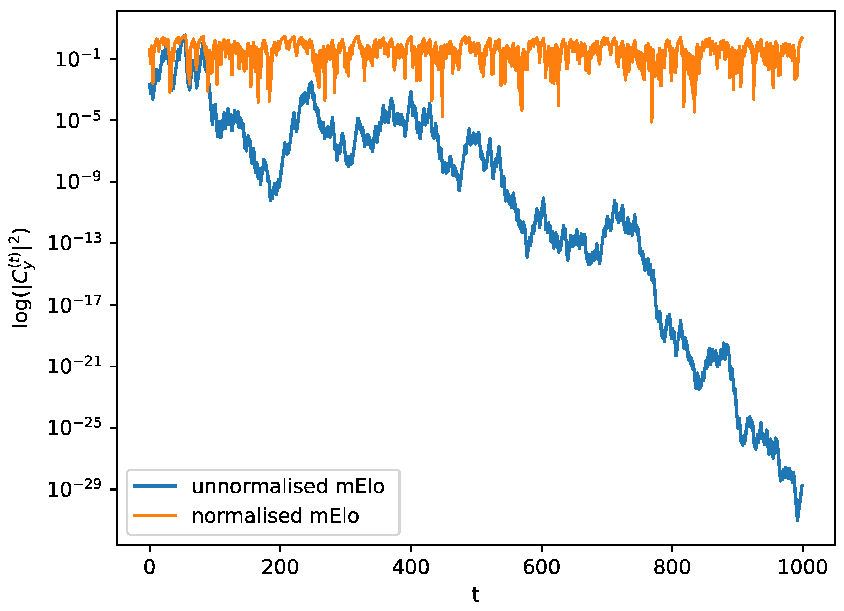
Figure 2.
A visual proof that the problem of fitting mElo vectors is under-determined. We fix the values of the mElo vectors A and B, and then we show that the vectors C and D cannot be uniquely determined. Because A can play C, we can observe the probability , hence we know the component of C perpendicular to A. This means that we know that C must lie on the line . Likewise, since we also observe the probability , we know that D must lie of the line . We can select any point on to be our vector C; we demonstrate this with two selections and . Because we can observe , we can draw the line parallel to our choice of C and where this line intersects is the location of D. Our choices of and lead to two different values of D, and . Both choices of C and D satisfy all given constraints.
Figure 2.
A visual proof that the problem of fitting mElo vectors is under-determined. We fix the values of the mElo vectors A and B, and then we show that the vectors C and D cannot be uniquely determined. Because A can play C, we can observe the probability , hence we know the component of C perpendicular to A. This means that we know that C must lie on the line . Likewise, since we also observe the probability , we know that D must lie of the line . We can select any point on to be our vector C; we demonstrate this with two selections and . Because we can observe , we can draw the line parallel to our choice of C and where this line intersects is the location of D. Our choices of and lead to two different values of D, and . Both choices of C and D satisfy all given constraints.
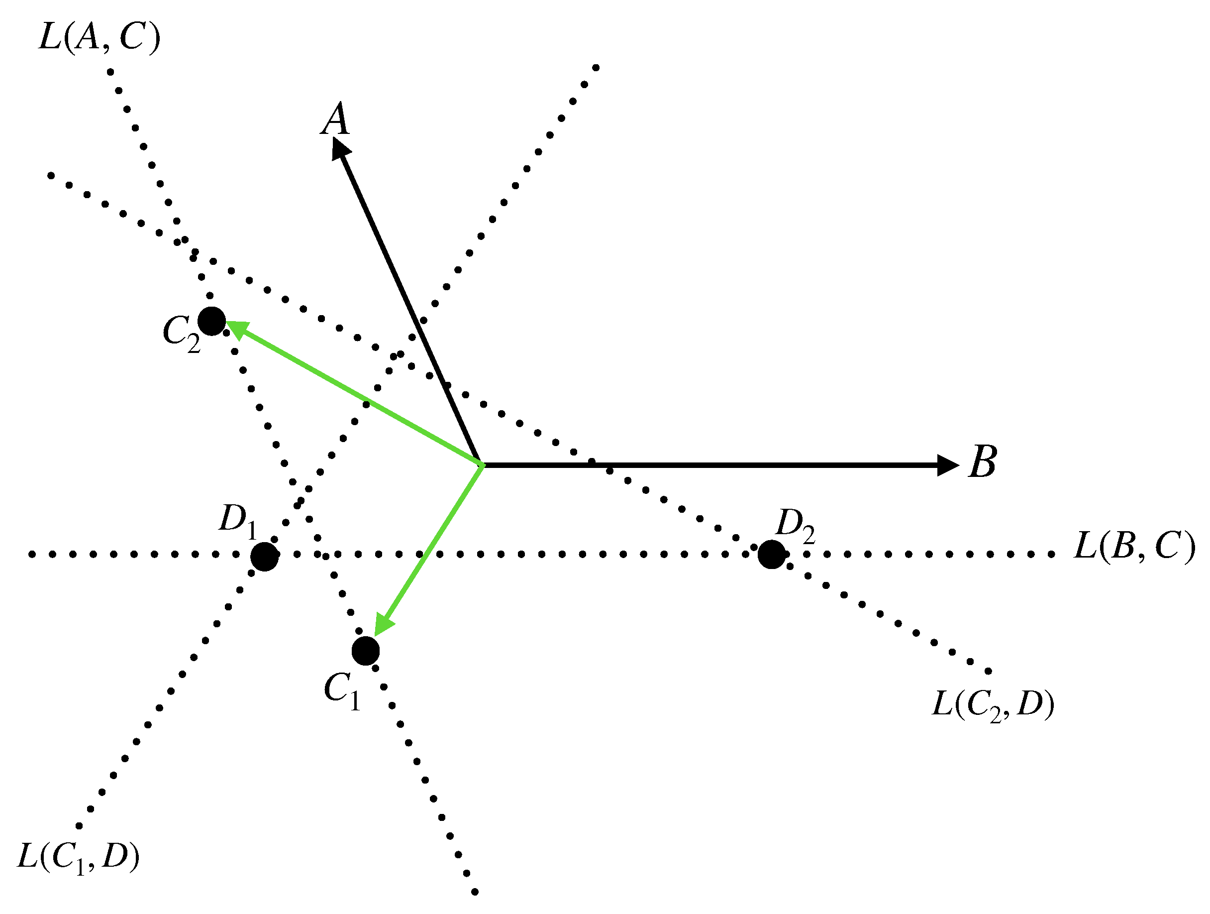
Figure 3.
The log-likelihood functions associated with the four scenarios described in Section 7.2. Each figure describes the log-likelihood of the value of , given fixed values of , , and . We can see that only in Scenario 4 is comparable to the set .
Figure 3.
The log-likelihood functions associated with the four scenarios described in Section 7.2. Each figure describes the log-likelihood of the value of , given fixed values of , , and . We can see that only in Scenario 4 is comparable to the set .
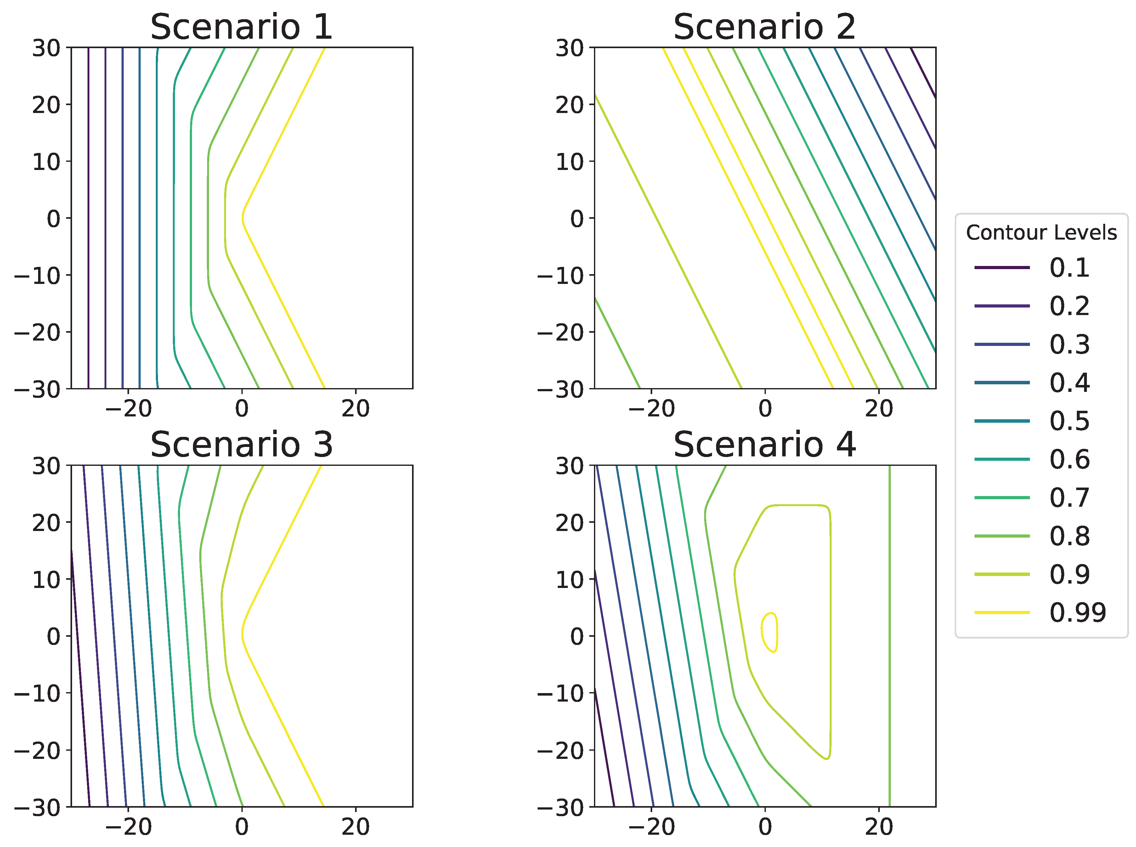
Figure 4.
Plot of the trajectories of the players’ mElo ratings over the course of the simulation The players initial mElo ratings are.
Figure 4.
Plot of the trajectories of the players’ mElo ratings over the course of the simulation The players initial mElo ratings are.
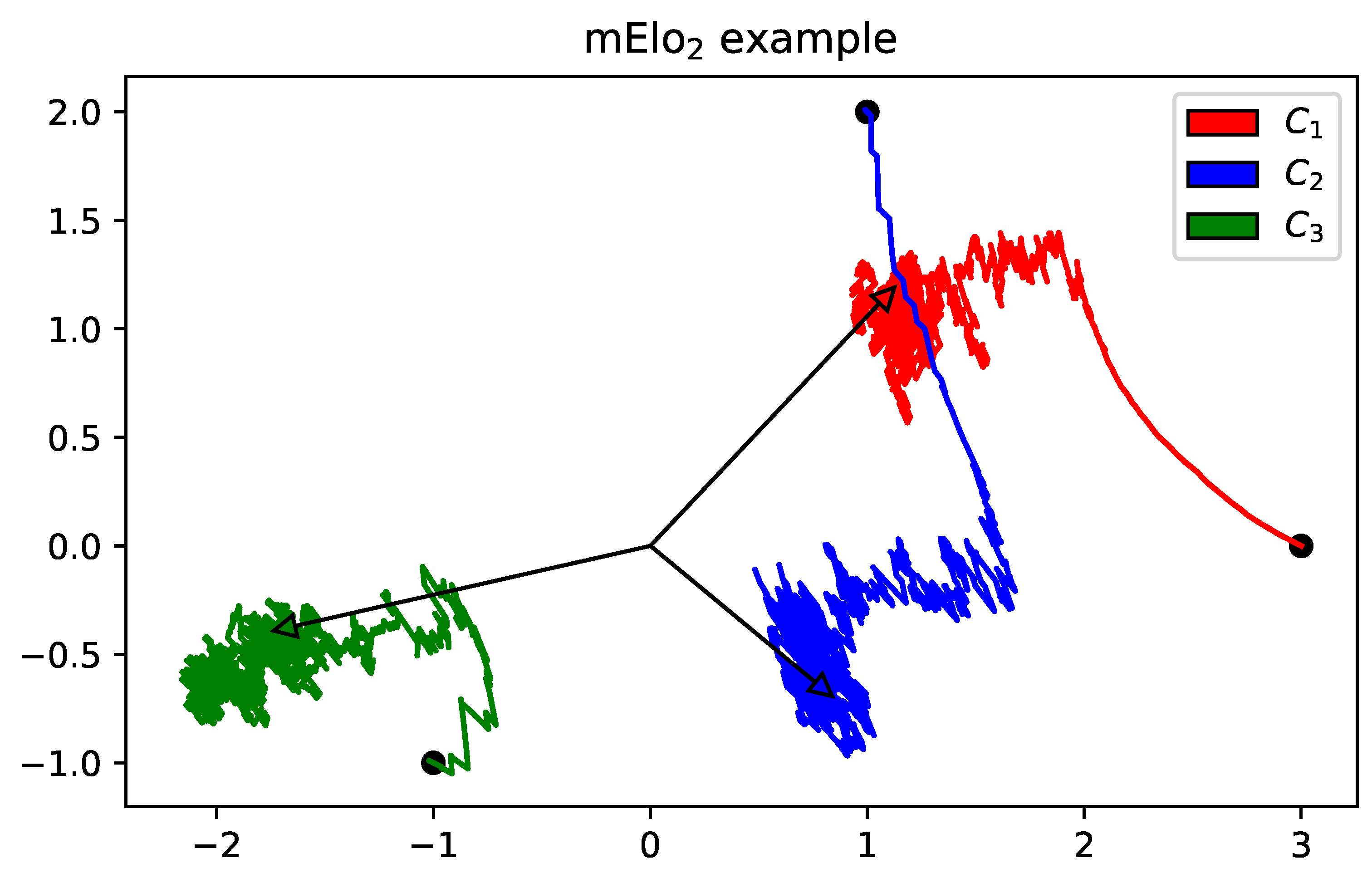
Figure 5.
Diagram of the Frobenius norm between the empirical expected payoff matrix and the true expected payoff matrix at each step during the simulation. We can see that the mElo rating system does approximate the true expected payoff matrix as required, but there will always be noise present at a certain level.
Figure 5.
Diagram of the Frobenius norm between the empirical expected payoff matrix and the true expected payoff matrix at each step during the simulation. We can see that the mElo rating system does approximate the true expected payoff matrix as required, but there will always be noise present at a certain level.
Disclaimer/Publisher’s Note: The statements, opinions and data contained in all publications are solely those of the individual author(s) and contributor(s) and not of MDPI and/or the editor(s). MDPI and/or the editor(s) disclaim responsibility for any injury to people or property resulting from any ideas, methods, instructions or products referred to in the content. |
© 2026 by the authors. Licensee MDPI, Basel, Switzerland. This article is an open access article distributed under the terms and conditions of the Creative Commons Attribution (CC BY) license (http://creativecommons.org/licenses/by/4.0/).
Copyright: This open access article is published under a Creative Commons CC BY 4.0 license, which permit the free download, distribution, and reuse, provided that the author and preprint are cited in any reuse.


