

Submitted:
29 May 2026
Posted:
02 June 2026
You are already at the latest version
Abstract
The present paper explores the inherent algebraic and geometric relation between the operations of scale-shift, i.e.~zoom, and rotation in representation space composed of the space and spectrum cardinal dimensions. Specifically, the fractional Fourier transform and a reversible meridian-step scale-shift are two facets---sharing the cyclic meridian index \( \Phi_t \) and its four cardinal interpretations---of one finite cyclic rotation in representation space, exact over the symmetry-complete prime shells \( F_p,\ p=4t+1 \) of the Finite Ring Continuum framework. Three theorems carry the meridian cycle of length \( p-1 \): (i) an FRC-native FrFT family, additive in the meridian index, reaching Fourier quarter-turn, parity, and inverse quarter-turn before returning to identity at the four cardinal meridians; (ii) a finite-field Weil realization in \( \mathrm{SO}(2,F_p) \) matching it on the cardinal Fourier sub-skeleton; (iii) a reversible scale-shift \( S_r:x\mapsto e_t^r x \) on \( F_p \)that recasts framed-rational refinement as a coordinate-side rotation. The same algebraic structure implies physical interpretation as chronon-indexed finite Schrödinger evolution, as well as Hubble-like cosmic dilation at the two opposed ends of the epistemic horizon. The construction is finite and algebraic; no continuum angle, trigonometric kernel, or limit is invoked.
Keywords:
fractional Fourier transform
; finite fields
; symmetry-complete shell
; cyclic rotation
; finitefield Weil dictionary
; meridian-coordinate zoom
; reversible scale shift
; finite ring cosmology
1. Introduction
The classical Fourier transform is usually described as a change of the basis of representation for both continuous and discrete signals. In its conventional analytic setting it exchanges a spatial variable with its spectral variable and satisfies the four-cycle
where P is parity. The fractional Fourier transform (FrFT) extends this four-cycle by interpreting the Fourier transform as a quarter-turn in representation space and by introducing intermediate rotated representations. This point of view appears in the work of Namias and in later optical and signal-processing treatments of the FrFT [1,2,3,4,5,6]. In the usual language these rotations are described as time-frequency rotations. In the present paper the corresponding shell terminology is spatial-spectral: the temporal/frequency vocabulary belongs to latitudinal phase analysis, while the meridional construction developed below rotates between spatial and spectral representation domains.
The aim of this paper is to define the FrFT exactly over a symmetry-complete finite fields that are defined in [7,8]. The specific setting is the finite shell
with prime. The multiplicative group then has order and contains a canonical quarter-turn subgroup once a primitive generator is chosen. Setting
gives . This is the finite shell analogue of the complex quarter-turn. The same shell datum also gives the half-period
The framed shell and its meridian-latitude geometry were introduced in earlier FRC work as a finite Euclidean shell layer in which the roles of e, , and i are reconstructed from finite arithmetic data [7,8]. In particular, the discrete shell Fourier transform used below is introduced in ([8] §6, Remark 13), where the representational reading of one Fourier step as a quarter-turn between primal and dual shell domains is also previewed and deferred to subsequent work ([8] end of §6); the present paper realizes that preview. Here we use only the finite-field layer: the cyclic group , its generator , the induced quarter-turn , and the meridian cycle .
Figure 1 shows a concrete shell visualization in the case . The meridians and latitudes correspond to the additive and the multiplicative actions of the orbital complex, while “Observer” marks the observer’s origin. The red meridian is the prime meridian and the blue meridian is the spectral meridian .
The main claim is that every shell meridian is a representation domain. The prime meridian is the spatial domain. The meridian , obtained by multiplying the meridian direction by , is the spectral domain. The meridian is the parity domain, and is the inverse-spectral domain. The finite FrFT is then the exact transform that rotates the representation from to .
The paper has three layers. The first is the FRC-native finite-field FrFT on the representation side, constructed by Theorem 1 (additivity and cardinal values) and completed by Theorem 2 (faithfulness on the full meridian cycle for ). The second is the finite-field Weil dictionary of Theorem 4, which matches the FRC-native family to the Weil realization on the cardinal Fourier skeleton. The third is the meridian-coordinate zoom of Theorem 3, which reads the same meridian cycle on the shell-coordinate side: the multiplicative map on sends the meridian to , and in a local comparison chart where is read as a real scale factor this is the algebraic form of reversible zoom-out by factor , while the inverse shift is the corresponding zoom-in. The finite-field map is a bijection of ; lossy coarse-graining appears only after an observer readout is added.
To begin with the first layer, let
and let
Define the shell Fourier matrix by
Since in , one obtains , where J is parity. The normalized operator
satisfies
The projectors onto the four eigenspaces of are polynomials in :
They define the finite fractional Fourier family
This family is additive in the meridian index:
It also has the required cardinal values
The Weil dictionary relates this FRC-native construction to the finite-field Weil interpretation on the cardinal Fourier skeleton. The classical Weil representation realizes symplectic transformations of a finite phase plane as operators on a finite state space; the Fourier transform is the operator associated with the Weyl quarter-turn element [9,10]. Recent work on arithmetic FrFTs similarly defines finite fractional Fourier transforms from finite arithmetic rotation groups [11]. In the present setting the FRC constants give an exact dictionary. For , set
Then
and is a group isomorphism from the meridian cycle to the finite-field rotation group for the form . Thus, the FRC meridian index and the finite-field Weil rotation index are the same finite datum written in two coordinate languages. This is the exact transfer supplied by , , and .
The construction is deliberately finite. It does not approximate a real angle. It replaces the continuum angle by the shell meridian index . It also avoids the ambiguity of arbitrary fractional powers of a discrete Fourier matrix. The projectors in () are canonical polynomials in the normalized finite Fourier operator.
2. Classical Fractional Fourier Transform
The classical FrFT is often introduced as a family of transforms such that
and
The angle-indexed convention is related to the iterate-indexed convention of equation (1) by ; the cardinal values match in the two readings. The analytic kernel contains functions such as and , but those functions are not the structural core. The structural core is the representation-space rotation. This observation is important because a finite-field construction has no need for a real angle or a trigonometric kernel. It needs only a finite cyclic rotation law with a Fourier quarter-turn.
The terminology used in this paper is as follows. A meridian of the shell is a representation axis. A latitude of the shell carries phase-cycle data. Hence, the meridional FrFT constructed here moves between spatial and spectral representation domains. The names temporal and frequency are not used for the meridional domains. They belong to a different layer of shell analysis, namely the latitudinal phase-cycle reading.
By a representation domain of the shell, in this paper, we shall always mean a basis-change pair on the same finite module , indexed by a meridian , where the meridional basis is obtained from the standard basis by the finite FrFT constructed below (see Definition 5). This is an internal definition: it refers only to the finite-field FrFT and its meridian index, with no auxiliary chart-level interpretation.
The intended finite replacement of the continuum angle is
only as an external comparison. Internally, the index is simply
Thus, the values correspond to the four cardinal representation domains.
3. Symmetry-Complete Shell Data
A symmetry-complete shell, in the sense used here, is a prime with , presented together with the framed datum where and is a chosen primitive generator. This is the FRC programme shell setting introduced in [7] and developed in [8]; the present paper uses only its finite-field layer.
Let be prime. The group is cyclic of order . Choose a primitive generator
Define the oriented quarter-turn by
The opposite primitive fourth root of unity is ; the choice of fixes the orientation, and we take throughout, consistent with ([8] §4). Then
by Euler’s criterion, since is primitive. The quarter-turn subgroup is
The half-period is
Remark 1
(Dependence on the choice of ). The construction below depends on the choice of primitive generator . Any other admissible choice has the form with . Under this change, the meridian relabelling realises the corresponding generator covariance of the framed shell established in ([8] Propositions 1–3); the FrFT family constructed below is therefore canonical relative to the framed datum rather than relative to alone.
The meridian index group is
For each , the meridian direction is . In an observer-framed shell one may write the meridian as
where is the finite meridian-step interval. For the operator construction of §§ 4–6 the precise choice of endpoint convention for is irrelevant; the meridian index s is the essential representation-domain label. For the meridian-coordinate zoom of § 7 we fix the convention .
Definition 1
(Cardinal meridians). The four cardinal meridians are
This definition records the intended shell reading. The rest of the paper proves that the finite Fourier and fractional Fourier operators realize exactly this meridional cycle at the representation level.
4. The Normalized Shell Fourier Operator
Let
Vectors in are functions . Define the reversal operator by
Clearly .
Definition 2
(Shell Fourier matrix). The shell Fourier matrix is the linear operator with entries
Equivalently,
This is a finite-field Fourier transform over the cyclic phase group . It is internal to because is a root of unity of order in . The same matrix is recorded as the shell DFT in ([8] §6, Remark 13); the present section adds only the shell quarter-turn normalization and the resulting four-cycle.
Lemma 1.
The shell Fourier matrix satisfies
Proof.
For ,
If , then every summand is 1 and the sum is in . If , then and the finite geometric sum is
Therefore, exactly when and 0 otherwise. This is precisely . □
Definition 3
(Normalized shell Fourier quarter-turn). Define
The normalization by is forced by the shell constants: is the quarter-turn already present in the symmetry-complete field.
Proposition 1.
The normalized shell Fourier operator satisfies
Proof.
Using Lemma 1 and ,
Since , it follows that . □
Thus, is an exact finite quarter-turn: one application gives the spectral representation, two applications give parity, and four applications return to the original representation.
5. Canonical Finite Fractional Powers
A direct fractional power of a Fourier matrix can be non-canonical if eigenspaces have multiplicity and an arbitrary eigenbasis is chosen. The construction below avoids this issue by using projectors that are polynomials in itself.
Since and , the polynomial splits in as
with four distinct roots. Define
Here denotes the inverse of 4 in .
Lemma 2.
The operators are pairwise orthogonal idempotents satisfying
and
Proof.
This is the standard idempotent decomposition of the cyclic group algebra after adjoining all fourth roots of unity. A direct verification uses the finite character orthogonality identity
The relation follows by multiplying (15) by and reindexing powers modulo 4. □
Definition 4
(FRC-native finite FrFT). For each meridian index , define
This is the central definition of the paper. The continuum angle has been replaced by a finite meridian index, and the four eigenvalues of the Fourier quarter-turn have been refined from to .
Theorem 1
(Exact finite-field FrFT). The family is a cyclic representation of the meridian group . In particular,
for all . Moreover,
Consequently, is an exact -th root of the normalized shell Fourier transform:
Proof.
Using Lemma 2,
This proves additivity. For the cardinal values, use . Then
because is the eigenspace projector for . Similarly,
and
Finally, , hence . The root identity follows from additivity:
□
The cardinal values of Theorem 1 are correct without faithfulness; they only require the four projectors and the additivity. The full -domain reading, however — the statement that every shell meridian gives a representation domain distinct from the others — requires the family to be injective on . Injectivity in turn requires the four eigenprojectors to be individually nonzero. In characteristic zero this would be automatic, but over a verification is needed. The remainder of this section supplies it.
Lemma 3
(Symmetric/antisymmetric decomposition). The Fourier matrix commutes with the reversal:
and hence so does . Decompose
with
Then stabilizes , with
Proof.
For ,
which gives the commutation. The involution J acts on by with fixed points and pairs. Hence and . Stabilization follows from the commutation, and gives the eigenvalues on . □
Lemma 4
(Multiplicity). Write for . Then
For every , and . For every , and . At () the antisymmetric subspace is one-dimensional, so exactly one of is zero; but is exhausted by the cardinal indices in that case, so no intermediate meridian is lost.
Proof.
The first two identities follow from Lemma 3: is the sum of the eigenspaces of (eigenvalues , , ), while is the sum of the eigenspaces (eigenvalues ).
For the eigenvalue pair on , consider the symmetric vector . Then for every k, so , the all-ones vector. Thus has nonzero entries at every index , whereas has support . Consequently , so is not a scalar operator. Since , the minimal polynomial of divides ; as it has degree at least 2, it equals and both eigenvalues occur. Hence and .
For the eigenvalue pair on with , consider the antisymmetric vector . Then
which vanishes iff , iff , iff . For the index lies outside and satisfies since has order . Hence , while , so and is not a scalar. Since , its minimal polynomial divides and equals this product, so both eigenvalues occur. Hence and .
For , , so is a scalar; that scalar squares to , hence equals either or , and exactly one of is zero. □
Theorem 2
(Faithfulness on the meridian cycle). For , the map
is injective. In particular, the meridional images are pairwise distinct.
Proof.
Suppose . Multiplying by and using together with for gives
By Lemma 4, for . Taking therefore gives , and since has order in , this forces . □
6. Meridional Representation Domains
We now state the representation-domain reading. Let be the standard basis of , interpreted as the coordinate basis of the prime spatial domain.
Definition 5
(Meridional representation domain). For , the operator is invertible: its eigenvalues () are nonzero powers of in , so has nonzero determinant. Define the meridional basis
The meridional representation domain is the pair
Thus all domains use the same finite module , but each domain writes its coordinates in a different meridional basis. The transform from to is
Corollary 1
(Cardinal domains). The four cardinal domains are
The parity domain sits at meridian index , identifying the role of the half-period in the dictionary.
Proof.
The statement follows immediately from Theorem 1. At , the basis is unchanged. At , the basis is transformed by the normalized Fourier quarter-turn. At , the basis is transformed by parity J. At , the basis is transformed by the inverse Fourier quarter-turn. □
Corollary 2
(Distinct representation domains). For , the meridional representation domains are pairwise distinct.
Proof.
By Theorem 2, the map is injective for , so the meridional bases are pairwise distinct, and hence so are the pairs . □
This proves the first main thesis: shell meridian rotation is represented algebraically as rotation in representation space.
7. Meridian-Coordinate Zoom
The previous section read each meridian index on the representation side, as the basis-change pair acted on by . The present section reads the same meridian index on the coordinate side, as the subset acted on by multiplication by , and records the corresponding scale-shift law. The two readings live on opposite sides of the shell Fourier correspondence and are exact at the finite-field level. The scale-shift law recorded below is the FrFT-meridian repackaging of the framed-rational zoom and scale-periodicity established in ([7] §4.3, Lemma 2); the dictionary between the two formulations is given in Remark 2 below, and a visual depiction of the same -step zoom cycle at appears as Figure 7 of that paper.
For the zoom interpretation we fix the meridian-step interval
of cardinality . The meridian from (9) is then a labelled subset of , traversed in the order .
Definition 6
(Meridian-scale map). For , define
Since is a unit, each is a bijection of , with inverse . The collection is a cyclic group under composition.
Proposition 2
(Meridian-scale covariance). For all ,
In particular, the meridian shift multiplies the meridian direction by , and the meridian shift multiplies it by .
Proof.
Using Definition 6 and the meridian definition,
□
Remark 2
(Identification with the framed-rational zoom). Proposition 2 and the cyclic group are the FrFT-meridian repackaging of the framed-rational scale-periodicity developed in ([7] §4.3). In that setting, is presented as the coordinate ring of framed rationals
with a fixed primitive generator, and the zoom map is
The dictionary to the present section is
so that increasing the framed-rational scale level n by one — which divides the grid step by g, i.e. zoomsin— corresponds to the meridian shift , in agreement with the orientation convention of Theorem 3 below. The coordinate range used here is the meridian half-range; the algebra paper uses the full range . With these identifications, the -periodicity is exactly Lemma 2 of [7], which states on the framed-rational grids . A visual rendering of the resulting cyclic zoom ladder, drawn at , is Figure 7 of that paper; the textual zoom ladder of Example 1 below gives the same information for with primitive generator .
Corollary 3
(Effective shell step). The meridian realizes the prime-meridian coordinate vector at effective shell step :
Proof.
The elements of , listed by the ordering of , are for . The difference of consecutive entries in this ordering is , which is the effective step. □
To compare different meridians as scale-shifted copies of one another, we record an observer-side comparison chart, in the same spirit as the angle comparison introduced in Section 2.
Definition 7
(Local scale chart). Alocal scale chartfor the meridian frame is a partial comparison map in which the shell unit is represented by a positive real scale factor
Under this comparison, the effective shell step is read as the real scale step .
The chart adds no new finite-field structure. It supplies the external observer vocabulary in which the words “finer” and “coarser” acquire a meaning; itself carries no compatible global order.
Theorem 3
(Meridian zoom). Fix a local scale chart with . Then:
- (i)
- represents the meridian-coordinate vector at step 1.
- (ii)
- represents the same meridian-coordinate vector at step for every .
- (iii)
- The forward shift multiplies the local scale step by λ and is the algebraic form of zoom-out.
- (iv)
- The inverse shift multiplies the local scale step by and is the algebraic form of zoom-in.
The cardinal meridians are read as
Proof.
Item (i) is the case of Corollary 3, where the effective step is and the local-scale image is . Item (ii) is the general case of the same corollary together with Definition 7, which sends the effective shell step to . Items (iii) and (iv) follow because Proposition 2 gives , so the effective step is multiplied by , read as in the chart. The cardinal values are the cases . □
Remark 3
(Reversible zoom versus lossy coarse-graining). Each is a bijection of , so meridian zoom is reversible at the finite-field level: . A genuinely lossy coarse-graining requires an additional observer map: a bounded comparison window that discards points outside it, a resolution map that identifies nearby comparison-chart points, a projection from onto a smaller measured alphabet, or a truncation of the meridian-coordinate vector. The precise statement is therefore
meridian shift is exact reversible zoom; coarse-graining is zoom followed by observer readout.
This keeps the proposition algebraically exact while preserving the intended observational interpretation.
Example 1
(Meridian-step ladder at ). Let , , , , . The meridian-step interval is and the first four meridians of the zoom ladder are
The effective step doubles at every meridian shift, in agreement with Theorem 3 for . Starting from the listing wraps around ; the corresponding “coarser” reading is observer-local rather than a global order statement on .
Remark 4
(Scope of the unification). The meridian cycle carries two coherent algebraic readings: the representation-side rotation
faithful on the full cycle for by Theorem 2, and the coordinate-side scale shift
an exact reversible bijection for every r. The two families act on carriers of different dimension over — is -dimensional, while is one-dimensional over itself — and are therefore not equal as operators. What they share is the cyclic index group and the cardinal interpretations at , both built from the shell constants , , . The phrasing “two facets of one rotation” is therefore to be read at the cyclic-group level and at the level of cardinal labeling, with the operator-level unification — an explicit intertwining map relating on to on — recorded as the natural next target of the programme and left to future work.
The scale-shift interpretation of as multiplication by in a local scale chart holds in the zoom-like range , where the shell-value of the cumulative dilation remains below the radius parameter; outside that range, the same algebraic action wraps around and manifests as phase intermixing across the cycle rather than as a clean external scale shift. The coordinate-side reading was developed at the framed-rational level in ([7] §4.3, Lemma 2 and Figure 7); the present section recasts it in FrFT-meridian language so that the two layers share the same index group .
8. Finite-Field Weil Dictionary
The previous construction is internal to the cyclic shell Fourier structure over . We now connect it to the finite-field Weil reading.
Let carry the quadratic form
Because , the element exists in and . The corresponding rotation group is
For each meridian index , set
and define
Finally set
Lemma 5.
For every , .
Proof.
Since ,
Hence, preserves and has determinant 1. □
Proposition 3
(FRC constants parametrize finite rotations). The map
is a group isomorphism.
Proof.
The formulas (23) are exactly the change of variables
Multiplication of the elements and gives
Under the identification
multiplication of z corresponds to multiplication of matrices. Hence, . Since is primitive, is an isomorphism . The above identification gives , so is an isomorphism. □
The cardinal meridians become the usual finite quarter-turns:
Let denote the finite Weil representation of in a chosen Schrodinger model. We only need its restriction to and the standard fact that the Weyl element
is represented, up to the usual scalar convention, by the finite Fourier transform [9,10]. Fix the scalar convention so that and .
Definition 8
(Weil FrFT pulled back by FRC constants). Define
Definition 9
(Cardinal-skeleton equivalence of FrFT realizations). Two FrFT families and are calledcardinal-skeleton equivalentwhen there exists one cyclic index group such that both are representations of and the four cardinal elements are sent respectively to identity, Fourier quarter-turn, parity, and inverse Fourier quarter-turn in their corresponding state spaces.
This definition is intentionally representation-theoretic. It compares the order-4 Fourier sub-skeleton of and the cardinal interpretations attached to its four elements. It does not require the two realizations to act on vector spaces of the same dimension or over the same coefficient field. It also does not constrain the two families at intermediate (non-cardinal) meridian indices .
Theorem 4
(FRC–Weil cardinal-skeleton dictionary). The FRC-native FrFT family and the finite-field Weil FrFT family are cardinal-skeleton equivalent in the sense of Definition 9. The exact transfer is the dictionary
and on the cardinal indices
where the parity meridian uses the half-period . The dictionary identifies the order-4 Fourier sub-skeleton of inside .
Proof.
By Theorem 1, is a representation of with the cardinal values listed in (18). By Proposition 3, is an isomorphism . Since is a representation of , its restriction to makes a representation of the same cyclic group . The cardinal values follow from the explicit matrices , , , and together with the chosen Weil normalization. Therefore both families satisfy Definition 9. □
Remark 5
(Scope of the dictionary). Theorem 4 pins down agreement of the two FrFT families only on the four cardinal indices , which generate the order-4 Fourier sub-skeleton of . Two cardinal-skeleton equivalent families may therefore differ freely at intermediate meridian indices . Faithfulness of on the full meridian cycle is established separately by Theorem 2, but it is a statement about the FRC-native family in isolation rather than a comparison with the Weil family.
The FRC-native family acts on and is internal to the shell Fourier cycle. The standard Schrodinger model of the Weil representation usually acts on functions on the additive group with complex or cyclotomic coefficients. Genuine isomorphism of the two families is therefore unavailable: they act on spaces of different dimension over different coefficient rings. Equality of a chosen operator model at intermediate s is obtained only after selecting a common realization and a scalar convention.
9. Worked Example:
Let
The element is primitive in . Therefore,
and
The meridian cycle has twelve representation domains:
The cardinal domains are
The quarter-turn rotation matrix is obtained from . Since in ,
Thus,
On the coordinate side, the same shell gives the zoom ladder (step 1), (step 2), (step 4), (step 8), illustrating Theorem 3 at . The wrap-around visible from onward shows that “coarser” is an observer-local statement rather than a global order claim on .
The exact arithmetic checks used for this paper are shown in Table 1. The entries report exact modular computations; no floating-point arithmetic is involved.
10. Discussion and Conclusion
The construction gives a finite replacement for the continuum FrFT based on shell meridians rather than real angles. It has three immediate consequences.
First, the Fourier transform becomes a literal algebraic quarter-turn in representation space. The normalization is essential: the unnormalized ring Fourier matrix satisfies , while the normalized shell operator satisfies and hence realizes the standard Fourier-parity four-cycle exactly.
Second, the fractional transforms are canonical. They are not arbitrary choices of fractional matrix powers. The projectors are polynomials in , and the replacement is fixed by the shell generator . Thus the one-step transform is an exact -th root of the shell Fourier quarter-turn.
Third, the finite-field Weil interpretation is not external to the shell. The constants , , and give the exact passage from a meridian index to a finite-field rotation matrix. The same element can be read as a shell meridian, as the nonzero field element , or as the rotation ; on the four cardinal indices it can also be read as the Weil operator , and Theorem 4 establishes the FRC-native and Weil families as cardinal-skeleton equivalent. At intermediate meridian indices the two readings act on spaces of different dimension over different coefficient rings, and are not required to coincide.
Fourth, the meridian cycle has a coordinate-side counterpart to the representation-side rotation. Multiplication by sends to exactly, and in any local scale chart this realizes the meridian step as a reversible zoom: forward shift coarsens the local step, inverse shift refines it. The finite-field map is a bijection of ; lossy coarse-graining requires an additional observer readout. The meridian cycle of a symmetry-complete shell therefore admits three coherent readings of one common index: a representation-side rotation , faithful on the full cycle for ; a finite-field Weil rotation , cardinal-skeleton equivalent to the FRC-native family; and a coordinate-side reversible zoom , exact at the finite-field level. The first two are linked by the cardinal-skeleton dictionary; connecting the first and third in a single intertwining theorem is a natural target for future work.
Physical interpretation The continuum FrFT is established as the evolution operator of the quantum harmonic oscillator, acting as the propagator at time [1]. The finite meridian rotation described by Theorem 1 therefore admits a natural reading as a finite, chronon-indexed Schrödinger evolution on the symmetry-complete shell, with the four-cycle as its closure. A finite Schrödinger–Dirac formalism built on exactly this shell rotation is developed in [12]. Furthermore, Theorem 3 invites a parallel cosmological reading: in any local scale chart , the meridian shift realizes a uniform exponential dilation by factor per chronon step, so the meridian cycle supplies an exact finite analogue of a Hubble-like expansion of the scale frame. Establishing this reading as a viable physical theory will require extensive dedicated programmatic work and is left to future research on both wave-function-level, and the cosmological extremes of the epistemological scale.
In conclusion, for every symmetry-complete prime shell , the framed datum determines an exact finite-field fractional Fourier transform. The prime meridian is the spatial domain. The quarter-turn meridian is the spectral domain. The half-turn meridian is the parity domain. For , every intermediate meridian is a genuinely distinct intermediate representation domain.
The main algebraic construction is
where the projectors are canonical polynomials in the normalized finite Fourier quarter-turn . This family satisfies exact additivity, exact cardinal values, and exact periodicity, and is faithful on the meridian cycle whenever .
The finite-field Weil interpretation is equivalent on the cardinal Fourier sub-skeleton. The shell constants provide the transfer
and Theorem 4 matches the FRC-native and Weil families on the four cardinal meridians . The two readings are not literally equal on the full cycle, because they act on spaces of different dimension over different coefficient rings; what they share is the order-4 Fourier sub-skeleton and its cardinal interpretation.
The coordinate-side reading of the meridian cycle is supplied by Theorem 3: the multiplicative map , , sends to , and in a local scale chart this becomes reversible meridian-step zoom-out (or zoom-in, for the inverse shift). The same meridian index therefore admits a representation-side reading, a Weil rotation reading, and a coordinate-side scale-shift reading, all derived from the framed shell datum .
Author Contributions
The sole author conceived the study, developed the formalism, carried out the proofs, performed the literature review, prepared the figures, and wrote the manuscript.
Funding
This research received no external funding.
Data Availability Statement
No new empirical data were created or analysed in this study.
Acknowledgments
The author thanks early readers for comments on earlier versions of this manuscript.
Conflicts of Interest
Author Yosef Akhtman was employed by the company Gamma Earth Sàrl and declares that the research was conducted in the absence of any commercial or financial relationships that could be construed as a potential conflict of interest.
References
- Namias, V. The Fractional Order Fourier Transform and its Application to Quantum Mechanics. IMA J. Appl. Math. 1980, 25, 241–265. [Google Scholar] [CrossRef]
- Almeida, L.B. The Fractional Fourier Transform and Time-Frequency Representations. IEEE Trans. Signal Process. 1994, 42, 3084–3091. [Google Scholar] [CrossRef]
- Ozaktas, H.M.; Mendlovic, D. Fourier Transforms of Fractional Order and their Optical Interpretation. Opt. Commun. 1993, 101, 163–169. [Google Scholar] [CrossRef]
- Ozaktas, H.M.; Arikan, O.; Kutay, M.A.; Bozdagi, G. Digital Computation of the Fractional Fourier Transform. IEEE Trans. Signal Process. 1996, 44, 2141–2150. [Google Scholar] [CrossRef]
- Candan, C.; Kutay, M.A.; Ozaktas, H.M. The Discrete Fractional Fourier Transform. IEEE Trans. Signal Process. 2000, 48, 1329–1337. [Google Scholar] [CrossRef]
- Ozaktas, H.M.; Zalevsky, Z.; Kutay, M.A. The Fractional Fourier Transform with Applications in Optics and Signal Processing; Wiley, 2001. [Google Scholar]
- Akhtman, Y. Relativistic Algebra over Finite Ring Continuum. Axioms 2025, 14, 636. [Google Scholar] [CrossRef]
- Akhtman, Y. Geometry and Constants in Finite Ring Continuum. Symmetry 2026, 18, 751. [Google Scholar] [CrossRef]
- Weil, A. Sur certains groupes d’operateurs unitaires. Acta Math. 1964, 111, 143–211. [Google Scholar] [CrossRef]
- Gurevich, S.; Hadani, R. The Geometric Weil Representation, 2006. arXiv arXiv::math.RT/math/0610818.
- Floratos, E.; Pavlidis, A. A Novel Finite Fractional Fourier Transform and its Quantum Circuit Implementation on Qudits. arXiv 2024, arXiv:quant-ph/2409.05759. [Google Scholar]
- Akhtman, Y. Schrödinger–Dirac Formalism in Finite Ring Continuum, 2026. Preprint. [CrossRef]
Figure 1.
Observer-framed visualization of the orbital shell for the symmetry-complete prime shell . Meridians are additive orbits, orange latitudes are multiplicative orbits, “Observer” is the observer’s origin. The red and blue meridians are the prime meridian and the quarter-turn meridian .
Figure 1.
Observer-framed visualization of the orbital shell for the symmetry-complete prime shell . Meridians are additive orbits, orange latitudes are multiplicative orbits, “Observer” is the observer’s origin. The red and blue meridians are the prime meridian and the quarter-turn meridian .
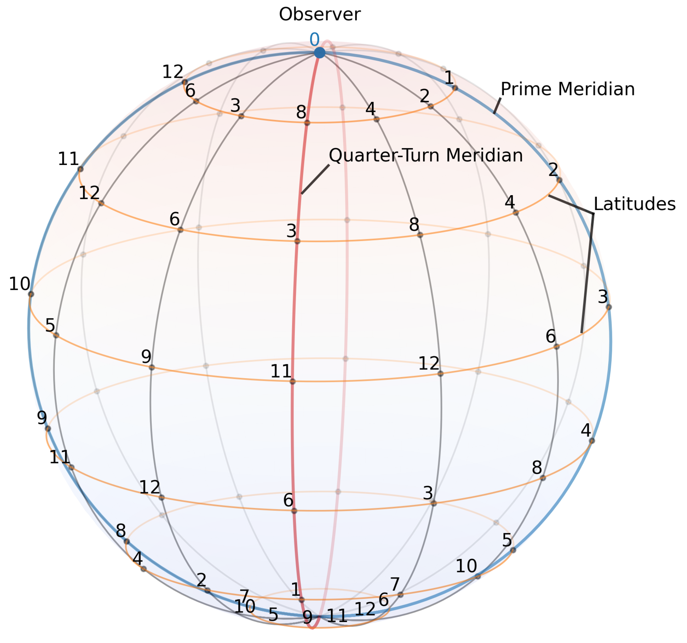

Table 1.
Exact modular validation of the finite Fourier and rotation identities for several symmetry-complete prime shells. The row is the degenerate case in which the meridian cycle is exhausted by the four cardinal indices and there are no intermediate meridians; the multiplicity Lemma 4 then leaves one of zero, but the faithfulness statement of Theorem 2 is vacuous in that case because no intermediate meridian needs to be distinguished. All rows with realize the full -domain reading.
Table 1.
Exact modular validation of the finite Fourier and rotation identities for several symmetry-complete prime shells. The row is the degenerate case in which the meridian cycle is exhausted by the four cardinal indices and there are no intermediate meridians; the multiplicity Lemma 4 then leaves one of zero, but the faithfulness statement of Theorem 2 is vacuous in that case because no intermediate meridian needs to be distinguished. All rows with realize the full -domain reading.
| 5 | 1 | 2 | 2 | true | true | true | |
| 13 | 3 | 2 | 8 | true | true | true | |
| 17 | 4 | 3 | 13 | true | true | true | |
| 29 | 7 | 2 | 12 | true | true | true | |
| 37 | 9 | 2 | 31 | true | true | true | |
| 41 | 10 | 6 | 32 | true | true | true |
Disclaimer/Publisher’s Note: The statements, opinions and data contained in all publications are solely those of the individual author(s) and contributor(s) and not of MDPI and/or the editor(s). MDPI and/or the editor(s) disclaim responsibility for any injury to people or property resulting from any ideas, methods, instructions or products referred to in the content. |
© 2026 by the authors. Licensee MDPI, Basel, Switzerland. This article is an open access article distributed under the terms and conditions of the Creative Commons Attribution (CC BY) license (http://creativecommons.org/licenses/by/4.0/).
Copyright: This open access article is published under a Creative Commons CC BY 4.0 license, which permit the free download, distribution, and reuse, provided that the author and preprint are cited in any reuse.


