Non-Existence of Global Smooth Solutions to the Navier–Stokes Equations in a 3D Periodic Domain with Prescribed Body Force

1. Introduction

The global regularity of the three-dimensional (3D) Navier–Stokes equations is one of the seven Millennium Prize Problems in mathematics (Fefferman 2006). For this topic, there are several studies in areas of partial differential equations (PDE) and mathematical fluid mechanics in recent decades. Although considerable efforts have been made, the problem remains neither proved nor disproved (Fioas et al. 2004). Leray (1934) constructed weak solutions and conjectured possible finite-time blow-up singularities. Ladyzhenskaya (1969) proved global smoothness for two-dimensional (2D) flows. For 3D flows, most studies focus on singularity due to velocity blow-up (Leray 1934; Serrin 1962; Caffarelli–Kohn–Nirenberg 1982). Bourgain and Pavlovic (2008) proved the ill-posedness of the Navier-Stokes equations in 3D critical functional space, which may result in the discontinuity of solutions for certain initial data. Tao (2016) suggested that finer structure of the nonlinearity should be considered if the regularity problem of the 3D Navier-Stokes equations is studied. Robinson (2020) reviewed the progress in this field, and concluded that the weak solution is able to sustained for the whole time, but the solution may not be unique, and the strong solution is unique, but can only extend a short time. Recently, Coiculescu and Palasek (2025) proved non-uniqueness of smooth solutions of the NavierStokes equations from critical data. The problem is still not resolved yet, although many efforts have been made in the community.

The difficulty of the problem lies in the fact that the behavior of the Navier-Stokes equations is closely tied to turbulence—one of the most complex and unresolved challenges in both mathematics and physics. With the rapid growth of computational resources, our understanding of turbulence has been greatly advanced by extensive simulation data, in addition to abundant experimental evidence (Dou, 2022). It is worth noting that the results of turbulent flow obtained from numerical simulations—such as Direct Numerical Simulation (DNS) and Large Eddy Simulation (LES)—show excellent agreement with experimental observations reported worldwide. Both experiments and simulations consistently indicate that the onset of turbulence depends on both the Reynolds number and the nature of the disturbance (Hof et al. 2003; Lemoult et al. 2012; Khan et al. 2020; Dou 2022). Therefore, any rigorous study on the regularity of the Navier-Stokes equations should properly account for the development of disturbances.

Recently, Dou (2025b, 2026) proved the non-existence of global smooth solutions for pressure-driven plane Poiseuille flow and for shear-driven plane Couette flow, respectively, with no-slip wall boundaries. In these studies, a new type of singularity is identified: regularity degeneration rather than velocity blow-up. This loss of regularity leads to the non-existence of global smooth solutions. The singularity emerges from a contradiction between the Energy-Velocity Monotonicity Principle (EVMP) and a non-vanishing incoming flow velocity, resulting in velocity discontinuity and a divergent velocity gradient.

Dou (2025b) established a theoretical framework to disprove the existence of global smooth solutions for the three-dimensional Navier–Stokes equations in pressure-driven flows. Specifically, for the classical plane Poiseuille flow, it was demonstrated that no global smooth solutions exist for the 3D incompressible Navier–Stokes equations. The breakdown of the solution is attributed not to velocity blow-up, but to a breakdown of regularity, which satisfies the well known BKM (Beale et al. 1984) breakdown criterion. Through the identification of singularities, velocity discontinuities, and spike formations, the singularities predicted by the Navier–Stokes equations are shown to align with the observed “negative velocity spikes” in turbulent transition. These theoretical findings are consistent with numerical simulations and experimental data for both wall bounded and free shear flows undergoing transition under influences of disturbance (Nishioka et al. 1975; Han et al. 2000; Niu et al. 2024; Zhou et al. 2025). The present study extends the above work to three-dimensional periodic domains under the action of smooth external forces.

For the Millennium problem, the solution is focused on mathematical analysis to decide whether smooth, physically reasonable solutions exist for the Navier–Stokes equations without effects from wall boundaries. It is asked for a proof of one of the four problem statements (Fefferman 2006). The forth statement (statement D) is described as: Breakdown of Navier–Stokes solutions on periodic domain ${\mathbb{R}}^3/{\mathbb{Z}}^3$. For 3D incompressible flow with fluid viscosity $\nu >0$, there exist a smooth, divergence-free initial vector field ${\mathit{u}}_0\left(x\right)$ and smooth scalar pressure field $p_0\left(x\right)$ on ${\mathbb{R}}^3$ as well as a smooth external force $f(x,t)$ on ${\mathbb{R}}^3\times [0,\infty )$, for which there exist no solutions $(\mathit{u},p)$ for Navier–Stokes equations on ${\mathbb{R}}^3\times [0,\infty )$.

In Dou (2025b, 2026), the computational domains are wall-bounded, and the influences of the boundaries are not excluded. In this study, a field of smooth external force is specifically constructed. We focus on the forth statement (statement D) in Fefferman (2006) to give a rigorous proof of the breakdown of Navier–Stokes solutions on ${\mathbb{R}}^3/{\mathbb{Z}}^3$ under smooth external force. This study adopts the identical theoretical frame of functional-analytic framework (Sobolev spaces, flow decomposition, EVMP, local viscous cancellation) as in Dou (2025b), and extend the theory to a periodic rectangular domain with prescribed smooth body force and smooth initial velocity and pressure fields. Then, we prove non-existence of global smooth solutions to the 3D Navier-Stokes equations for incompressible flow. We demonstrate how, in a laminar flow undergoing disturbance evolution at high Reynolds number, the velocity and its derivatives become discontinuous at a localized position, leading to a breakdown of the solution’s regularity.

2. Functional Setting and Periodic Domain

This section introduces the computational domain, periodic Sobolev function spaces, and the rigorous definition of global smooth solutions adopted throughout this paper.

2.1. Computational Domain and Periodic Boundaries

The flow is defined on a three-dimensional rectangular periodic domain embedded in the Euclidean space ${\mathbb{R}}^3$:

$$\Omega =(0,L_x)\times (-h,h)\times (-h,h)\subset {\mathbb{R}}^3$$

(1)

be a bounded smooth rectangular domain with periodic boundary conditions, and with lengths of the domain being $L_x$, $2h,$ and $2h$ in x, $y,$ and z directions, respectively.

The domain is equipped with full periodic boundary conditions in all three spatial directions, which is topologically equivalent to a three-dimensional torus:

$${\mathbb{T}}^3={\mathbb{R}}^3/{\mathbb{Z}}^3.$$

(2)

This topological equivalence guarantees the periodic extension of flow variables and eliminates boundary singularity interference.

The boundary conditions in all three directions are periodic:

$$\left\{\begin{array}{cc}& \mathit{u}(0,y,z,t)=\mathit{u}(L_x,y,z,t),{\partial }_x\mathit{u}(0,y,z,t)={\partial }_x\mathit{u}(L_x,y,z,t),\hfill \\ & \mathit{u}(x,-h,z,t)=\mathit{u}(x,h,z,t),{\partial }_y\mathit{u}(x,-h,z,t)={\partial }_y\mathit{u}(x,h,z,t),\hfill \\ & \mathit{u}(x,y,-h,t)=\mathit{u}(x,y,h,t),{\partial }_z\mathit{u}(x,y,-h,t)={\partial }_z\mathit{u}(x,y,h,t),\hfill \\ & p(0,y,z,t)=p(L_x,y,z,t),p(x,-h,z,t)=p(x,h,z,t),p(x,y,-h,t)=p(x,y,h,t).\hfill \end{array}\right.$$

(3)

Periodic boundaries eliminate the no-slip condition on solid walls, so the flow velocity can be ensured to be positive everywhere in $\Omega$.

2.2. Periodic Sobolev Spaces

For any non-negative integer $k\ge 0$, the periodic Sobolev space $H_{\mathrm{per}}^k(\Omega )$ is defined as the closure of all smooth periodic functions on $\Omega$ with finite $H^k$-norm (Adams and Fournier 2003; Brezis 2011; Taylor 2011; Evans 2010):

$$H_{\mathrm{per}}^k(\Omega )=\left\{f\in L^2(\Omega )|D^{\alpha }f\in L^2(\Omega ),\forall \left|\alpha \right|\le k,f\mathrm{periodic}\mathrm{on}\partial \Omega \right\},$$

where $\alpha$ denotes the multi-index derivative, and the standard Sobolev norm is defined by

$${\parallel f\parallel }_{H^k(\Omega )}={\left(\sum _{\left|\alpha \right|\le k}{\parallel D^{\alpha }f\parallel }_{L^2(\Omega )}^2\right)}^{1/2}.$$

(4)

The periodic Sobolev space $H_{\mathrm{per}}^k(\Omega )\subset H^k(\Omega )$ consists of functions satisfying periodicity on $\partial \Omega$.

The divergence-free periodic space is specified as

$$H_{\sigma ,\mathrm{per}}^k(\Omega )=\left\{\mathit{u}\in H_{\mathrm{per}}^k(\Omega )|\nabla ·\mathit{u}=0\right\}.$$

(5)

2.3. Definition of Global Smooth Solution

A velocity field $\mathit{u}(\mathit{x},t)$ is defined as a global smooth solution of the 3D Navier–Stokes system if it satisfies the following regularity conditions for all $t\in [0,+\infty )$:

$$\mathit{u}\in C\left([0,\infty );H_{\sigma ,\mathrm{per}}^3(\Omega )\right)\cap L_{\mathrm{loc}}^2\left([0,\infty );H^{k+1}(\Omega )\right),$$

(6)

( $k\ge 3$) and the uniform boundedness of velocity gradient holds:

$${\parallel \nabla \mathit{u}\left(t\right)\parallel }_{L^{\infty }(\Omega )}<\infty ,\forall t\ge 0.$$

(7)

The critical Sobolev embedding relation in three-dimensional space lays the foundation for smoothness judgment:

$$H^2(\Omega )\hookrightarrow L^{\infty }(\Omega ),H^3(\Omega )\hookrightarrow C^1\left(\overline{\Omega }\right).$$

(8)

This embedding indicates that any function with $H^3$ -regularity is continuously differentiable on the closed domain, without discontinuity or singular gradient.

3. Governing Equations and Flow Set Up

Figure 1. Schematic of periodical initial flow profile in rectangular duct with external force, ${\mathit{u}}_0(x,y,z)$. The origin of the coordinates is located at the centerline of the x-y cross-section; $y=h$ at upper boundary, and $y=-h$ at lower boundary; $z=h$ at front boundary, and $z=-h$ at back boundary.

Figure 1. Schematic of periodical initial flow profile in rectangular duct with external force, ${\mathit{u}}_0(x,y,z)$. The origin of the coordinates is located at the centerline of the x-y cross-section; $y=h$ at upper boundary, and $y=-h$ at lower boundary; $z=h$ at front boundary, and $z=-h$ at back boundary.

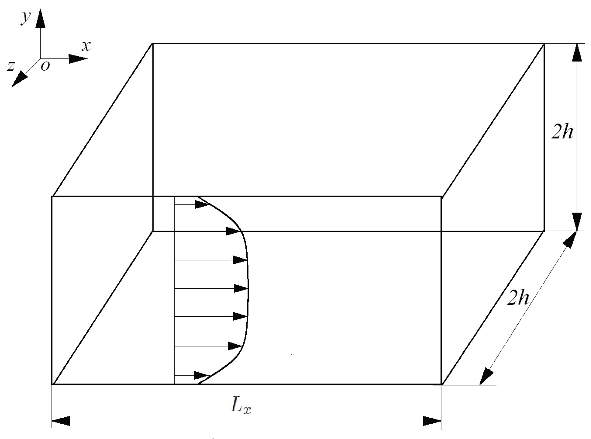
3.1. 3D Navier–Stokes Equations with Body Force

The system of governing equations for 3D incompressible viscous flow is:

$$\left\{\begin{array}{cc}{\displaystyle \frac{\partial \mathit{u}}{\partial t}}+(\mathit{u}·\nabla )\mathit{u}=-{\displaystyle \frac{1}{\rho }}\nabla p+\nu \Delta \mathit{u}+{\displaystyle \frac{1}{\rho }}\mathit{F},\hfill & \mathit{x}\in \Omega ,t>0,\hfill \\ \nabla ·\mathit{u}=0,\hfill & \mathit{x}\in \Omega ,t>0,\hfill \\ \mathit{u}{|}_{\partial \Omega }\mathrm{is}\mathrm{periodic},\hfill \\ \mathit{u}(\mathit{x},0)={\mathit{u}}_0\left(\mathit{x}\right),\hfill & \mathit{x}\in \Omega .\hfill \end{array}\right.$$

(9)

Notation:

- $\mathit{u}=(u_x,u_y,u_z)$: velocity vector

- $\mathit{x}=(x,y,z)$: position vector

- $\rho >0$: density of fluid

- $\nu ={\displaystyle \frac{\mu }{\rho }}>0$: kinematic viscosity of fluid

- $\mu$: dynamic viscosity of fluid

- p: pressure

- $\mathit{F}$: prescribed body force ( $volumeforce$) of unit volume fluid

- $\Delta ={\partial }_x^2+{\partial }_y^2+{\partial }_z^2$: Laplacian operator.

The prescribed body force is given by

$$\mathit{F}={\mathit{F}}_1+{\mathit{F}}_2={\left({\displaystyle \frac{2\mu a}{h^2}},0,0\right)}^T+{\left({\displaystyle \frac{12\mu b}{h^4}}{y}^2,0,0\right)}^T.$$

(10)

where ${\mathit{F}}_1$ is the conservative body force, and ${\mathit{F}}_2$ is the non-conservative body force. The body force $\mathit{F}$ is designed so that the stationary 2D problem admits an exact polynomial solution.

In Eq.(10),

$${\mathit{F}}_{\mathit{1}}={(F_{1x},F_{1y},F_{1z})}^T={\left({\displaystyle \frac{2\mu a}{h^2}},0,0\right)}^T$$

$${\mathit{F}}_{\mathit{2}}={(F_{2x},F_{2y},F_{2z})}^T={\left({\displaystyle \frac{12\mu b}{h^4}}{y}^2,0,0\right)}^T.$$

With Eq.(10), the momentum equation in Eq.(9) can be rewritten as,

$${\displaystyle \frac{\partial \mathit{u}}{\partial t}}+(\mathit{u}·\nabla )\mathit{u}=-{\displaystyle \frac{1}{\rho }}(\nabla p-{\mathit{F}}_1)+\nu \Delta \mathit{u}+{\displaystyle \frac{1}{\rho }}{\mathit{F}}_2,\mathit{x}\in \Omega ,t>0$$

(11)

It is seen from Eq.(11) that the conservative body force and the non-conservative body force may play different roles to the evolution of the flow.

3.2. Initial Condition and Reynolds number

3.2.1. Initial Conditions

For steady flow, the governing equations and the boundary conditions in a two-dimensional channel with no-slip boundary conditions gives an exact solution, from Eqs.(9) and (10),

$$u_x\left(y\right)=a(1-{\displaystyle \frac{y^2}{h^2}})+b(1-{\displaystyle \frac{y^4}{h^4}})$$

(12)

where a and b are given by Eqs.(9) and (10), and Eq.(12) is compatible with a smooth pressure field.

Let $h_1=1.10h$, the initial velocity field is extended uniformly in the z-direction, ${\partial }_z\mathit{u}\equiv 0$, with the following velocity distribution:

$$\left\{\begin{array}{c}{u}_x(\mathit{x},0)=a\left(1-{\displaystyle \frac{y^2}{h_1^2}}\right)+b\left(1-{\displaystyle \frac{y^4}{h_1^4}}\right),\hfill \\ u_y(\mathit{x},0)=0,\hfill \\ u_z(\mathit{x},0)=0.\hfill \end{array}\right.$$

(13)

Thus

$${\mathit{u}}_0\left(\mathit{x}\right)={\left(a\left(1-{\displaystyle \frac{y^2}{h_1^2}}\right)+b\left(1-{\displaystyle \frac{y^4}{h_1^4}}\right),0,0\right)}^T.$$

(14)

The initial pressure field is given by $p(\mathit{x},0)=p_0\left(\mathit{x}\right)=0$, which is compatible with Eq.(14), and the pressure period boundary conditions are expressed as in Eq.(3).

The initial velocity field ${\mathit{u}}_0$ has the following properties:

1. ${\mathit{u}}_0\in C^{\infty }\left(\overline{\Omega }\right)$, smooth.

2. $\nabla ·{\mathit{u}}_0=0$, divergence-free.

3. ${\mathit{u}}_0\in H_{\sigma ,\mathrm{per}}^3(\Omega )$.

4. $\left|\right({\mathit{u}}_0{|}_{\partial \Omega }\left)\right|>0$, and the minimum of $\left|\right({\mathit{u}}_0{|}_{\partial \Omega }\left)\right|$ occurs at $y=\pm h=\pm 0.9091h_1$ ( due to $h_1=1.10h$).

5. $u_x(\mathit{x},0)={\mathit{u}}_0\left(\mathit{x}\right)·\mathit{i}>0$ everywhere in $\Omega$, and $\mathit{i}$ is the unit vector in x direction. This property is realized by adopting fully periodic boundary conditions, which avoid the zero-velocity limitation on solid walls and ensure the velocity field remains positive over the entire domain without boundary attenuation.

On the y-z cross-sectional boundaries of the periodic domain, the initial velocity defined by Eq.(14) is strictly positive. This initial profile eliminates all wall-imposed no-slip constraints like that in traditional plane Poiseuille flow, thus excludes any influences from the boundaries.

3.2.2. Reynolds number

The Reynolds number in this study is defined as,

$$\mathrm{Re}={\displaystyle \frac{2h{U}_{x0}}{\nu }}$$

where $U_{x0}$ is the cross-sectional averaged velocity on the initial velocity profile along the x direction, h is the half width of the domain in both y and z directions, and $\nu$ is the kinematic viscosity. For plane Poiseuille flow, the critical value of the Reynolds number for turbulent transition, ${\mathrm{Re}}_{cr}=1506$, was obtained in Jovanovic and Pashtrapanska (2004, their Eq.(27) ), which agrees well with extensive experimental results (Dou 2022).

For the flow driven by external force in the periodic domain, expressed by Eq.(14), the critical Reynolds number may be slightly different. However, for parallel flows, there is a universal critical value of the energy gradient function $K_c=380$ (Dou 2022). With this $K_c=380$, the critical Reynolds number $\mathrm{Re}>{\mathrm{Re}}_{cr}$ can be obtained for the flow distribution expressed by Eq.(14), if the parameters a and b are given (Dou 2022). The range of the Reynolds number considered in this study is $\mathrm{Re}>{\mathrm{Re}}_{cr}$.

4. Velocity Decomposition in Sobolev Spaces

We decompose the instantaneous velocity into a time-averaged mean flow $\mathit{U}$ and a zero-mean disturbance $\mathit{v}$,

$$\mathit{u}(\mathit{x},t)=\mathit{U}(\mathit{x},t)+\mathit{v}(\mathit{x},t).$$

(15)

4.1. Time-Averaged Operator

The averaged velocity $\mathit{U}$ is defined as the time average over $[t-\Delta t/2,t+\Delta t/2]$:

$$\mathit{U}(\mathit{x},t)={\displaystyle \frac{1}{\Delta t}}{\int }_{t-\Delta t/2}^{t+\Delta t/2}\mathit{u}(\mathit{x},\mathit{\tau })d\mathit{\tau },$$

(16)

where

- $\Delta t\gg {\mathit{\tau }}_d$ (disturbance time scale),

- $\Delta t\ll t^{*}$ (first singularity time).

The disturbance velocity $\mathit{v}$ is defined as:

$$\mathit{v}=\mathit{u}-\mathit{U},{\displaystyle \frac{1}{\Delta t}}{\int }_{t-\Delta t/2}^{t+\Delta t/2}\mathit{v}\left(\mathit{\tau }\right)d\mathit{\tau }=0.$$

(17)

4.2. Regularity Inheritance

Since $\mathit{u}\in C([0,t^{*});H_{\sigma ,\mathrm{per}}^3(\Omega ))$ and the time-average operator is bounded linear on $H^3(\Omega )$:

$$\mathit{U}\in C\left([0,t^{*});H_{\sigma ,\mathrm{per}}^3(\Omega )\right).$$

(18)

Sobolev spaces are closed under subtraction:

$$\mathit{v}\in C\left([0,t^{*});H_{\sigma ,\mathrm{per}}^3(\Omega )\right).$$

(19)

4.3. Dominance of Mean Flow

For laminar evolution before singularity:

$${\parallel \mathit{U}\parallel }_{H^3(\Omega )}\gg {\parallel \mathit{v}\parallel }_{H^3(\Omega )},\underset{\Omega }{inf}\mathit{U}\ge C_0>0.$$

(20)

where $C_0$ is a positive constant. The mean flow remains uniformly positive owing to the applied body force, periodic boundary conditions and prescribed initial velocity field.

5. Preliminaries (Sobolev Space-Based Derivations)

5.1. Local Vanishing of the Sum of the Viscous Term and the non-conservative body force

In the following theorem, we prove that for the given conditions, there exists a point in the flow field where the sum of the viscous term and the non-conservative body force vanishes with the disturbance evolution,

$$\nu \Delta \mathit{u}+{\displaystyle \frac{1}{\rho }}{\mathit{F}}_2=0,\mathit{x}\in \Omega .$$

Theorem 5.1 (Local Vanishing of $\nu \Delta \mathit{u}+{\mathit{F}}_2/\rho$)

Let $\Omega \subset {\mathbb{R}}^3$ be the periodic rectangular domain defined above, and let $\mathit{u}\in C\left([0,t^{*});H_{\sigma ,\mathrm{per}}^3(\Omega )\right)$ be a local smooth solution to the 3D incompressible Navier–Stokes equations with smooth body force $\mathit{F}$ and smooth initial data.

Assume that $B_{ϵ}\left({\mathit{x}}^{*}\right)$ is an open subset $B_{ϵ}\left({\mathit{x}}^{*}\right)\in \Omega$ and the Reynolds number satisfies

$$\mathrm{Re}>{\mathrm{Re}}_{cr}.$$

Then, there exists a finite time $t^{*}>0$ and an interior point ${\mathit{x}}^{*}\in \Omega$ such that

$$\underset{t\to t^{*}}{lim}{∥\nu \Delta \mathit{u}(·,t)+{\displaystyle \frac{1}{\rho }}{\mathit{F}}_2(·,t)∥}_{H^1\left(B_{ϵ}\left({\mathit{x}}^{*}\right)\right)}=0.$$

(21)

That is, the sum of the viscous term and the non-conservative body force vanishes locally in the $H^1$-norm.

Proof

1. Linearity and Boundedness: Using the decomposition $\mathit{u}=\mathit{U}+\mathit{v}$ (Eq.15), the Laplacian is linear:

$$\Delta \mathit{u}=\Delta \mathit{U}+\Delta \mathit{v}$$

(22)

and by the regularity inheritance,

$$\mathit{U}\in H^3\Rightarrow \Delta \mathit{U}\in H^1,\Delta \mathit{v}\in H^1.$$

Since $\Omega$ is a bounded domain with periodic boundary conditions and $\mathit{U}\in H_{per}^3(\Omega )$, the Sobolev embedding theorem implies $H^3(\Omega )\hookrightarrow C^1\left(\overline{\Omega }\right)$. Hence $\Delta \mathit{U}\in C^0\left(\overline{\Omega }\right)$, and therefore $\Delta \mathit{U}$ is uniformly bounded on $\Omega$. The prescribed body force $\mathit{F}$ is also bounded and smooth.

2. Disturbance Amplification: For $\mathrm{Re}>{\mathrm{Re}}_{cr}$, the nonlinear convective term $(\mathit{U}·\nabla )\mathit{v}$ dominates. Since the gradient of the disturbance velocity is proportional to the mean velocity, the nonlinear term $(\mathit{U}·\nabla )\mathit{v}$ (which is one part of $(\mathit{u}·\nabla )\mathit{u}$) exponentially amplifies $\mathit{v}$ by the Sobolev product estimate. The disturbance velocity and its gradients grow without bound as $t\to t^{*}$:

$${\parallel (\mathit{U}·\nabla )\mathit{v}\parallel }_{H^2}\le C{\parallel \mathit{U}\parallel }_{H^3}{\parallel \nabla \mathit{v}\parallel }_{H^2}\sim C{\parallel \mathit{U}\parallel }_{H^3}{\parallel \Delta \mathit{v}\parallel }_{H^1}.$$

(23)

Consequently, the disturbance viscous term $\nu \Delta \mathit{v}$ oscillates and its magnitude increases continuously.

3. Existence of the Cancellation Point ${\mathit{x}}^{*}$: Since $\mathit{U}\in H^3(\Omega )$ and $\Delta \mathit{U}(\mathit{x},t)\in H^1(\Omega )$, and $\Delta \mathit{U}(\mathit{x},t)$ is bounded in the domain, thus $\nu \Delta \mathit{U}(\mathit{x},t)+{\displaystyle \frac{1}{\rho }}{\mathit{F}}_2(\mathit{x},t)$ is also bounded in the domain. As $\mathrm{Re}>{\mathrm{Re}}_{cr}$, the disturbance Laplacian $\Delta \mathit{v}$ oscillates and grows continuously by the amplification of the nonlinear convective term.

By Eqs.(9), (10) and (11), $\nu \Delta \mathit{U}(\mathit{x},t)+{\displaystyle \frac{1}{\rho }}{\mathit{F}}_2(\mathit{x},t)$ is negative over the compact domain $\Omega$ before reaching $({\mathit{x}}^{*},t^{*})$. The disturbance term $\nu \Delta \mathit{v}(\mathit{x},t)$ oscillates and takes both positive and negative values over time. The most possible time for $\nu \Delta \mathit{v}(\mathit{x},t)$ to firstly offset $\nu \Delta \mathit{U}(\mathit{x},t)+{\displaystyle \frac{1}{\rho }}{\mathit{F}}_2(\mathit{x},t)$ is at the positive maximum of $\nu \Delta \mathit{v}(\mathit{x},t)$ in a period (when $\partial (\nu \Delta \mathit{v})/\partial t=0$). The most possible position for this cancelling must occur at the point where the maximum disturbance increase takes place.

Since $\nu \Delta \mathit{v}(\mathit{x},t)$ oscillates in sign and grows unboundedly, while $\nu \Delta \mathit{U}({\mathit{x}}^{*},t^{*})+{\mathit{F}}_2({\mathit{x}}^{*},t^{*})/\rho$ is smooth and bounded, there must exist $({\mathit{x}}^{*},t^{*})$ ($\partial (\nu \Delta \mathit{v})/\partial t=0$ at $t^{*}$) such that,

$$\nu \Delta \mathit{v}({\mathit{x}}^{*},t^{*})=-\left(\nu \Delta \mathit{U}({\mathit{x}}^{*},t^{*})+{\displaystyle \frac{1}{\rho }}{\mathit{F}}_2({\mathit{x}}^{*},t^{*})\right).$$

(24)

4. Cancellation: Substituting the above identity into Eq.(22) yields the pointwise cancellation at $({\mathit{x}}^{*},t^{*})$:

$$\nu \Delta \mathit{u}({\mathit{x}}^{*},t^{*})+{\displaystyle \frac{1}{\rho }}{\mathit{F}}_2({\mathit{x}}^{*},t^{*})=0.$$

(25)

5. Limit in $H^1$-norm: By the continuity of the $H^1$-norm and the pointwise convergence established above, the local $H^1$-norm of the sum tends to zero:

$$\underset{t\to t^{*}}{lim}{∥\nu \Delta \mathit{u}(·,t)+{\displaystyle \frac{1}{\rho }}{\mathit{F}}_2(·)∥}_{H^1\left(B_{ϵ}\left({\mathit{x}}^{*}\right)\right)}=0.$$

It is important to note that this cancellation requires the two vector terms to be collinear, acting along the same line but pointing in opposite directions.

5.2. Determination of Points Where the Sum of Viscous Term and Non-Conservative Body Force Vanishes

Theorem 5.2 (Position of Local Vanishing of $\nu \Delta \mathit{u}+{\mathit{F}}_2/\rho$)

Let $\Omega \subset {\mathbb{R}}^3$ be the periodic rectangular domain, and let $\mathit{u}\in C([0,t^{*});H_{\sigma ,\mathrm{per}}^3(\Omega ))$ be a local smooth solution of the 3D incompressible Navier–Stokes equations with smooth external force $\mathit{F}={\mathit{F}}_1+{\mathit{F}}_2$.

Assume that the Reynolds number satisfies

$$\mathrm{Re}>{\mathrm{Re}}_{cr}.$$

Then there exists a finite time $t^{*}>0$ and a point ${\mathit{x}}^{*}\in \Omega \setminus \partial \Omega$ (i.e., an interior point) such that

$$\nu \Delta \mathit{u}({\mathit{x}}^{*},t^{*})+{\displaystyle \frac{1}{\rho }}{\mathit{F}}_2({\mathit{x}}^{*},t^{*})=0.$$

Consequently, the local vanishing of the sum of the viscous term and the non-conservative body force occurs strictly in the interior of the domain.

Further, the position of $({\mathit{x}}^{*},t^{*})$ coincides with the maximum of the energy gradient function K. As such, the position of $({\mathit{x}}^{*},t^{*})$ can be determined by the maximum of K.

Proof

By Theorem 5.1, for $\mathrm{Re}>{\mathrm{Re}}_{cr}$ there exist $t^{*}>0$ and ${\mathit{x}}^{*}\in \Omega$ such that Eq.(21) holds,

$$\underset{t\to t^{*}}{lim}{∥\nu \Delta \mathit{u}(·,t)+{\displaystyle \frac{1}{\rho }}{\mathit{F}}_2(·)∥}_{H^1\left(B_{ϵ}\left({\mathit{x}}^{*}\right)\right)}=0.$$

Since the periodic domain $\Omega$ has no boundary in the usual sense, the vanishing occurs away from the physical boundary, if it occurs.

1. Disturbance Amplification by the Nonlinear Convective Term. By the Theorem 5.1, the position at which the sum of the viscous term and the non-conservative body force vanishes is associated with the maximum of the disturbance increase.

The nonlinear convective term can be rewritten as follow with the velocity decomposition (Eq.(15)),

$$(\mathit{u}·\nabla )\mathit{u}=(\mathit{U}·\nabla )\mathit{U}+(\mathit{U}·\nabla )\mathit{v}+(\mathit{v}·\nabla )\mathit{U}+(\mathit{v}·\nabla )\mathit{v}$$

(26)

The second term on the right hand side of above equation, $(\mathit{U}·\nabla )\mathit{v}$, is the dominating term among the four terms to amplify the disturbance, where $\nabla \mathit{v}$ is proportional to the mean velocity $\mathit{U}$. For $\mathrm{Re}>{\mathrm{Re}}_{cr}$, $(\mathit{U}·\nabla )\mathit{v}$ leads to exponential increase of the disturbance (Schmid and Henningson 2001). According to Eq.(26), the position of the maximum disturbance increase corresponds to the place of the maximum of $\left|\right(\mathit{u}·\nabla \left)\mathit{u}\right|$ taking place.

2. The Energy Gradient Function Characterizing the Interplay between the Nonlinear Convective Term and the Viscous Term.

In the Navier-Stokes equations, the nonlinear convective term amplifies disturbances, while the viscous term provides a damping effect. The dimensionless parameter characterizing the balance and interplay between these two mechanisms is the energy gradient function K in the energy gradient theory (Dou 2022). For flows with no external work input (e.g., pressure-driven or body force-driven flows), K is expressed as follows for parallel flow when $\partial \mathit{u}/\partial t=0$ (at the extreme values of disturbance velocity):

$$K=\left|{\displaystyle \frac{\partial E/\partial y}{\partial E/\partial x}}\right|=\left|{\displaystyle \frac{\partial p/\partial y+\rho u_x\partial u_x/\partial y}{\partial E/\partial x}}\right|$$

(27)

where $E=p+{\displaystyle \frac{1}{2}}\rho {\left|\mathit{u}\right|}^2+F_{1x}x$ is the total mechanical energy (see Eqs.(9), (10) and (11)). The energy gradient function K represents a local Reynolds number (Dou 2022). This function characterizes the local competition between nonlinear convection and viscous diffusion.

For the initial flow distribution given by Eq.(14), $\partial E/\partial x$ is constant along y direction. By comparing Eq.(26) and Eq.(27), it is seen that the maximum of $|\mathit{u}·\nabla \mathit{u}|$ (also means the maximum of $|\mathit{U}·\nabla \mathit{U}|$) in the initial flow corresponds to the maximum of K since $p\left(y\right)$ is constant. As such, the maximum disturbance increase occurs at the position with maximum of K. Then, we are able to use K to charaterize the position of local vanishing of $\nu \Delta \mathit{u}+{\mathit{F}}_2/\rho$ (and it will be shown later it corresponds to the singularity).

3. Calculation of Position of $Kmax$. For the initial velocity distribution given by Eq.(14), the calculation of K can be carried out by Eq.(27), see Table 1. Here, the values of $Kmax$ are normalized by the Reynolds number. For $a=1,b=0$, the maximum of K occurs at $y/h=\pm 0.5774$. For $a=0,b=1$, the maximum of K occurs at $y/h=\pm 0.8100$. For any combinations of a and b, the maximum of K occurs in the range of $\pm 0.5774\sim \pm 0.8100$, which is located interior of the domain.

It is seen that the energy gradient function K attains its maximum in the interior of the domain (see Table 1), which coincides with the position where the disturbance is most strongly amplified. Therefore, $x^{*}$ is an interior point of $\Omega$, and Eq.(21) holds interior of the domain ${\mathit{x}}^{*}\in \Omega \setminus \partial \Omega$.

Meanwhile, the periodic boundary conditions rule out boundary-induced singularities, further confirming that the vanishing point of $\nu \Delta \mathit{u}+{\mathit{F}}_2/\rho$ and the generated singularity are strictly interior points of $\Omega$. Therefore, the Theorem 5.2 is proved.

For an instance, if we set $a=1,b=0.20$ in Eq.(14), let ${\displaystyle \frac{\partial K}{\partial y}}=0$, then, we obtain that the maximum of K occurs at,

$$y/h=\pm 0.6430$$

(28)

Thus, $y/h=\pm 0.6430$ are the positions to have the maximum disturbance increase corresponding to $a=1,b=0.20$, where $\nu \Delta \mathit{u}+{\mathit{F}}_2/\rho =0$. If the disturbance is amplified sufficiently, singularities will be produced there ($y/h=\pm 0.6430$), which will be demonstrated later.

It is emphasized that the formula for K employed in this section (Eq.(27))—and consequently the determination of its maximum position—is strictly valid only for flow configurations without external work input. If external work input were considered (e.g. plane Couette flow), the expression for K would require modification (Dou 2022).

5.3. Energy–Velocity Monotonicity Principle (EVMP)

Theorem 5.3 (Local Vanishing of $\nu \Delta \mathit{u}+{\mathit{F}}_2/\rho$ Leads to Zero Velocity )

Let $\Omega \subset {\mathbb{R}}^3$ be the periodic rectangular domain, and let $\mathit{u}\in C([0,t^{*});H_{\sigma ,\mathrm{per}}^3(\Omega ))$ be a local smooth solution of the 3D incompressible Navier–Stokes equations with smooth external force $\mathit{F}={\mathit{F}}_1+{\mathit{F}}_2$.

Assume that at a point $({\mathit{x}}^{*},t^{*})\in \Omega \times (0,\infty )$, the following two conditions hold:

$${\displaystyle \frac{\partial \mathit{u}({\mathit{x}}^{*},t^{*})}{\partial t}}=0\mathrm{and}\mu \Delta \mathit{u}({\mathit{x}}^{*},t^{*})+({\mathit{F}}_2({\mathit{x}}^{*},t^{*})·\mathit{\tau }({\mathit{x}}^{*},t^{*}))\mathit{\tau }({\mathit{x}}^{*},t^{*})=0,$$

(29)

where $\mathit{\tau }={\displaystyle \frac{\mathit{u}}{\left|\mathit{u}\right|}}$ denotes the unit tangent vector along the streamline, defined for $t<t^{*}$ when $\mathit{u}\ne 0$.

Table 1. Variations of $K_{max}/Re$ and its position $y/h$ versus b for $a=1.$ in initial flow field

No.	b	$\pm y/h$	$Kmax/Re$
1	0.0	0.5774	0.7697
2	0.1	0.6050	0.9352
3	0.2	0.6430	1.1275
4	0.3	0.6650	1.3448
5	0.4	0.6870	1.5878
6	0.5	0.7030	1.8564
7	0.6	0.7100	2.1501
8	0.8	0.7300	2.8128
9	1.0	0.7400	3.5739
10	2.0	0.7700	8.8478
11	5.0	0.7900	39.224
12	10.0	0.8000	138.31
13	50.0	0.8060	3110.0
14	100.0	0.8100	12272.
15	1000.0	0.8100	1212346.
16	10000.0	0.8100	121085767.

Table 1. Variations of $K_{max}/Re$ and its position $y/h$ versus b for $a=1.$ in initial flow field

No.	b	$\pm y/h$	$Kmax/Re$
1	0.0	0.5774	0.7697
2	0.1	0.6050	0.9352
3	0.2	0.6430	1.1275
4	0.3	0.6650	1.3448
5	0.4	0.6870	1.5878
6	0.5	0.7030	1.8564
7	0.6	0.7100	2.1501
8	0.8	0.7300	2.8128
9	1.0	0.7400	3.5739
10	2.0	0.7700	8.8478
11	5.0	0.7900	39.224
12	10.0	0.8000	138.31
13	50.0	0.8060	3110.0
14	100.0	0.8100	12272.
15	1000.0	0.8100	1212346.
16	10000.0	0.8100	121085767.

Then the total mechanical energy gradient satisfies

$$\nabla E({\mathit{x}}^{*},t^{*})cos\alpha =0,$$

(30)

and consequently

$$\mathit{u}({\mathit{x}}^{*},t^{*})=0.$$

(31)

The time derivative $\partial \mathit{u}/\partial t=0$ may occur in two cases, in steady flow and at the extreme values of disturbance velocity in unsteady flow.

Proof

The momentum equation (Eq.(11)) can be rewriten as (Dou 2022),

$$\rho {\displaystyle \frac{\partial \mathit{u}}{\partial t}}+\nabla E=\rho (\mathit{u}\times \nabla \times \mathit{u})+\mu \Delta \mathit{u}+{\mathit{F}}_2,(\mathit{x},t)\in \Omega \times (0,\infty )$$

(32)

where

$$E=p+{\displaystyle \frac{1}{2}}\rho {\left|\mathit{u}\right|}^2+F_{1x}x$$

(33)

is the total mechanical energy.

Projecting Eq.(32) onto the streamline direction $\mathit{\tau }$ yields,

$$\rho {\displaystyle \frac{\partial \mathit{u}}{\partial t}}+\nabla Ecos\alpha =\mu \Delta \mathit{u}+({\mathit{F}}_2·\mathit{\tau })\mathit{\tau },(\mathit{x},t)\in \Omega \times (0,\infty )$$

(34)

where $\alpha$ is the angle between $-\nabla E$ and $\mathit{u}$.

Since ${\partial }_t\mathit{u}=0$ at $({\mathit{x}}^{*},t^{*})$ and $\mu \Delta \mathit{u}+({\mathit{F}}_2·\mathit{\tau })\mathit{\tau }=0$ by Eq.(29), then Eq.(34) reduces to,

$$\nabla Ecos\alpha =0.$$

which is Eq.(30).

Physically, this means that no mechanical energy gradient is available to sustain motion along the streamline. Since the flow is viscous and no external work is supplied to the fluid element at $({\mathit{x}}^{*},t^{*})$, the only admissible solution compatible with the Navier–Stokes equations is the vanishing of velocity:

$$\mathit{u}({\mathit{x}}^{*},t^{*})=0.$$

Thus, the theorem 5.3 is proved.

It is very clear from the proof that the Theorem 5.3 is a direct analytical (algebraic) result of the Navier-Stokes equations, and there are no any additional conditions or assumptions.

It is pointed out here that

$$\mu \Delta \mathit{u}+{\mathit{F}}_2=0\iff \mu \Delta \mathit{u}+({\mathit{F}}_2·\mathit{\tau })\mathit{\tau }=0.$$

As mentioned before, mutual cancellation of the two terms implies that the vectors are collinear, lying on the same line and pointing in opposite directions.

5.4. Beale-Kato-Majda (BKM) criterion

Beale et al. (1984) proposed a criterion for the breakdown of smooth solutions to the 3D Euler equation, which is now known as the Beale-Kato-Majda (BKM) criterion. This criterion relates the solution breakdown to the growth of the vorticity norm as well as the time integration of the vorticity norm. In later studies, this criterion is extended to the Navier-Stokes equations (Kozono and Taniuchi 2000; Zhao 2017; Gibbon et al. 2018). Vorticity is defined as $\mathit{\omega }=\nabla \times \mathit{u}$, which reflects the rotational characteristics of the fluid.

Lemma 5.1 (BKM Criterion): Let $\mathit{u}\left(t\right)$ be a smooth solution of the 3D incompressible Navier-Stokes equations on $[0,t^{*})$, with the initial vorticity ${\mathit{\omega }}_0=\nabla \times {\mathit{u}}_0\in L^1(\Omega )\cap L^{\infty }(\Omega )$. If the solution diverges at $t=t^{*}$ (i.e., its regularity breaks down), then the following integral tending to infinity:

$${\int }_0^{t^{*}}{\parallel \mathit{\omega }\left(s\right)\parallel }_{L^{\infty }(\Omega )}d\tau =\infty$$

(35)

Otherwise, if the integral is finite, the solution can be smoothly extended beyond $t^{*}$.

6. Main Results

6.1. Singularity Formation via Regularity Degeneration

The central result of this study is the demonstration of a finite-time singularity in the 3D Navier–Stokes equations. Crucially, this singularity is not manifested as a divergence of kinetic energy (or velocity blow-up), but rather as a loss of differentiability (regularity degeneration). We establish this through the following logical steps.

6.1.1. Uniform Boundedness of the Kinetic Energy

We first confirm that the solution remains physically admissible. The Sobolev embedding theorem guarantees that functions in $H^2(\Omega )$ are continuous and bounded. Specifically, for the velocity field $\mathit{u}(\mathit{x},t)$ before $\mathit{u}({\mathit{x}}^{*},t^{*})$, we have:

$$H^2(\Omega )\hookrightarrow L^{\infty }(\Omega )$$

.

This implies the existence of a constant $C>0$ such that:

$${\parallel \mathit{u}\left(t\right)\parallel }_{L^{\infty }(\Omega )}\le C{\parallel \mathit{u}\left(t\right)\parallel }_{H^2(\Omega )}.$$

Combined with the Leray energy inequality (Leray 1934), above equation ensures that the velocity magnitude remains uniformly bounded for all $t\ge 0$. Consequently, any potential singularity must be a regularity singularity, not a velocity blow-up.

6.1.2. Local Regularity Breakdown of Solutions in the Interior Domain

Definition 6.1 (Finite-Time Interior Regularity Singularity)

Let $\Omega \subset {\mathbb{R}}^3$ be the periodic rectangular domain, and let $\mathit{u}\in C([0,t^{*});H_{\sigma ,\mathrm{per}}^3(\Omega ))$ be a local smooth solution of the 3D Navier–Stokes equations.

A point $({\mathit{x}}^{*},t^{*})\in \Omega \times (0,\infty )$ is called a finite-time interior regularity singularity if the following two conditions hold simultaneously:

(1) Vanishing of $H^3$-regularity. There exists a radius $ϵ>0$ such that

$$\underset{t\to t^{*}}{lim}{\parallel \mathit{u}(·,t)\parallel }_{H^3\left(B_{ϵ}\left({\mathit{x}}^{*}\right)\right)}=0.$$

(36)

(2) Uniform positivity of the $L^{\infty }$-norm. There exists a constant $C_0>0$ such that

$$\underset{t\in [0,t^{*})}{inf}{\parallel \mathit{u}(·,t)\parallel }_{L^{\infty }\left(B_{ϵ}\left({\mathit{x}}^{*}\right)\right)}\ge C_0.$$

(37)

where $B_{ϵ}\left({\mathit{x}}^{*}\right)\subset \Omega$ is an open subset with radius $ϵ$ of interior point ${\mathit{x}}^{*}\in \Omega$, $C_0$ is a positive constant, and $t^{*}>0$ is a finite time.

The coexistence of (36) and (37) constitutes a contradiction: the solution must vanish at $({\mathit{x}}^{*},t^{*})$ by $H^3$-regularity, yet it remains uniformly non-zero by the flow dynamics. Consequently, the solution cannot belong to $H^3$ at $({\mathit{x}}^{*},t^{*})$, and the Sobolev embedding $H^3(\Omega )\hookrightarrow C^1\left(\overline{\Omega }\right)$ fails locally. Such a point is defined as a finite-time interior regularity singularity of the Navier–Stokes equations.

Theorem 6.1 (Finite-Time Interior Regularity Singularity)

Let $\Omega \subset {\mathbb{R}}^3$ be the periodic rectangular domain defined above, and let $\mathit{u}\in C\left([0,t^{*});H_{\sigma ,\mathrm{per}}^3(\Omega )\right)$ be a local smooth solution to the 3D incompressible Navier–Stokes equations with smooth body force $\mathit{F}$ and smooth initial data.

Suppose

$$\underset{t\to t^{*}}{lim}\parallel \mathit{S}{\parallel }_{H^1\left(B_{ϵ}\left({\mathit{x}}^{*}\right)\right)}=0,\mathit{S}=\mu \Delta \mathit{u}+\left({\mathit{F}}_2·\mathit{\tau }\right)\mathit{\tau },$$

(38)

where $\mathit{\tau }=\mathit{u}/\left|\mathit{u}\right|$ is the unit streamline tangent vector, $B_{ϵ}\left({\mathit{x}}^{*}\right)\subset \Omega$ is an open subset with radius $ϵ$ of interior point ${\mathit{x}}^{*}\in \Omega$, and $t^{*}>0$ is a finite time.

Then the point $({\mathit{x}}^{*},t^{*})$ satisfies Definition 6.1; that is, $\mathit{u}$ loses $H^3$-regularity at $({\mathit{x}}^{*},t^{*})$, and a finite-time interior regularity singularity is formed at $({\mathit{x}}^{*},t^{*})$.

Proof

Assume, for contradiction, that $\mathit{u}\in H^3(\Omega )$ up to time $t^{*}$.

1. Vanishing of $\mathit{u}$ in $H^3\left(B_{ϵ}\left({\mathit{x}}^{*}\right)\right)$ at $t=t^{*}$

By assumption, $t\to t^{*}$ corresponds to an extremum of the disturbance velocity $\mathit{v}$, so that

$${\displaystyle \frac{\partial \mathit{u}}{\partial t}}({\mathit{x}}^{*},t^{*})=0.$$

Combining condition Eq.(38) with Theorem 5.3 (Energy–Velocity Monotonicity Principle), we obtain the vanishing limit in the $H^3$-norm:

$$\underset{t\to t^{*}}{lim}\parallel \mathit{u}(·,t){\parallel }_{H^3\left(Bϵ\left({\mathit{x}}^{*}\right)\right)}=0.$$

By norm continuity, the trace at the critical time is well defined and satisfies

$$\parallel \mathit{u}(·,t^{*}){\parallel }_{H^3\left(B_{ϵ}\left({\mathit{x}}^{*}\right)\right)}=0.$$

(39)

If $\mathit{u}(·,t^{*})\in H^3\left(B_{ϵ}\left({\mathit{x}}^{*}\right)\right)$ continuously holds, the Sobolev embedding in three-dimensions,

$$H^3\left(B_{ϵ}\right)\hookrightarrow C^1\left({\overline{B}}_{ϵ}\right)$$

is compact. Consequently, ${\parallel \mathit{u}\left(t\right)\parallel }_{H^3\left(B_{ϵ}\right)}\to 0$ implies convergence in the $C^1$-norm:

$${\parallel \mathit{u}\left(t\right)\parallel }_{C^1\left(B_{ϵ}\right)}⟶0\mathrm{as}t\to t^{*}.$$

Therefore, at the critical point we obtain,

$$\mathit{u}({\mathit{x}}^{*},t^{*})=0,\nabla \mathit{u}({\mathit{x}}^{*},t^{*})=0.$$

2. Uniform Positivity of ${\parallel \mathit{u}(·,t)\parallel }_{L^{\infty }\left(B_{ϵ}\left(x^{*}\right)\right)}$ for $t\in [0,t^{*})$

From the flow setup and properties of mean flow:

$$\underset{\mathit{x}\in B_{ϵ}\left(x^{*}\right)}{inf}{\parallel \mathit{U}(·,t)\parallel }_{L^{\infty }\left(B_{ϵ}\left(x^{*}\right)\right)}\ge C_0>0,\forall ,t\in [0,t^{*}),$$

where $C_0>0$ is a positive constant. Benefiting from the periodic boundary conditions that eliminate wall no-slip constraints, together with the prescribed body force, the time-averaged mean flow maintains a strictly positive lower bound over the entire domain.

Meanwhile, prior to singularity formation, the disturbance velocity satisfies,

$${\parallel \mathit{v}(·,t)\parallel }_{L^{\infty }\left(B_{ϵ}\left(x^{*}\right)\right)}\ll {\parallel \mathit{U}(·,t)\parallel }_{L^{\infty }\left(B_{ϵ}\left(x^{*}\right)\right)},\forall ,t\in [0,t^{*}).$$

By the triangle inequality for $L^{\infty }$-norm:

$${\parallel \mathit{u}(·,t)\parallel }_{L^{\infty }\left(B_{ϵ}\left(x^{*}\right)\right)}\ge \parallel \mathit{U}(·,t){\parallel }_{L^{\infty }\left(B_{ϵ}\left(x^{*}\right)\right)}-\parallel \mathit{v}(·,t){\parallel }_{L^{\infty }\left(B_{ϵ}\left(x^{*}\right)\right)}>0,\forall ,t\in [0,t^{*}).$$

(40)

That is, $\mathit{u}(·,t)$ is uniformly non-vanishing in $L^{\infty }\left(B_{ϵ}\left(x^{*}\right)\right)$ for all time before $t^{*}$.

3. Contradiction between $H^3$ Regularity and $L^{\infty }$ Boundedness

At the critical time $t^{*}$ and interior point ${\mathit{x}}^{*}\in B_{ϵ}\left({\mathit{x}}^{*}\right)\subset \Omega$:

(1) From Eq.(39), $\mathit{u}\equiv \mathit{0}$ on $B_{ϵ}\left({\mathit{x}}^{*}\right)$ in the sense of $H^3$-regularity;

(2) From the time-continuity of the flow dynamics and Eq.(40): $\mathit{u}(\mathit{x},t)\not\equiv \mathbf{0}$ near ${\mathit{x}}^{*}$ for all $t<t^{*}$, and the flow field maintains positive magnitude locally approaching $({\mathit{x}}^{*},t^{*})$.

This yields a fundamental contradiction: the solution cannot simultaneously satisfy $\mathit{u}=0$ by $\mathit{u}\in H^3\left(B_{ϵ}\left({\mathit{x}}^{*}\right)\right)\mathrm{and}\mathit{u}\not\equiv \mathbf{0}$ by $L^{\infty }\left(B_{ϵ}\left(x^{*}\right)\right)$ boundedness $\mathrm{locally}\mathrm{near}{\mathit{x}}^{*}$ at $t=t^{*}$. This contradiction demonstrates that $\mathit{u}$ loses $H^3$-Sobolev regularity at $({\mathit{x}}^{*},t^{*})$.

These results satisfy the two conditions of definition in Definition 6.1 on regularity degeneration singularity of the Navier–Stokes solution at a finite time $t^{*}>0$ and an interior point ${\mathit{x}}^{*}\in \Omega$.

4. Breakdown of Sobolev Embedding and Formation of Regularity Singularity

For the 3D bounded domain $\Omega$, the standard Sobolev embedding theorem states: $H^3(\Omega )\hookrightarrow C^1\left(\overline{\Omega }\right).$ This embedding is a necessary condition for the existence of global classical $smooth$ solutions to the 3D Navier–Stokes equations: it guarantees that velocity $\mathit{u}$ and its first-order gradient $\nabla \mathit{u}$ are continuous on $\overline{\Omega }$.

Since $\mathit{u}$ loses $H^3$-regularity at $({\mathit{x}}^{*},t^{*})$, the embedding $H^3(\Omega )\hookrightarrow C^1\left(\overline{\Omega }\right)$ fails locally on $B_{ϵ}\left({\mathit{x}}^{*}\right)$. Consequently:

1. $\mathit{u}(·,t)$ loses continuity at ${\mathit{x}}^{*}$ as $t\to t^{*}$;

2. The gradient $\nabla \mathit{u}(·,t)$ loses continuity at ${\mathit{x}}^{*}$ as $t\to t^{*}$.

In the theory of partial differential equations, a point where a smooth local solution loses its maximal expected regularity is defined as a regularity singularity. Thus $({\mathit{x}}^{*},t^{*})$ is a finite-time interior regularity singularity of the Navier–Stokes solution.

In summary, the Navier–Stokes dynamics preserve the boundedness of $\mathit{u}$ (via $H^2(\Omega )\hookrightarrow L^{\infty }(\Omega )$) but fail to preserve the boundedness of $\nabla \mathit{u}$ as $t\to t^{*}$ (via the collapse of $H^3(\Omega )\hookrightarrow C^1\left(\overline{\Omega }\right)$). This establishes the formation of a finite-time, interior regularity singularity, and the solution cannot be extended as a global smooth solution beyond $t^{*}$.

6.2. Breakdown of Solutions at $({\mathit{x}}^{*},t^{*})$

The velocity gradient $L^{\infty }$-norm:

$${\parallel \nabla \mathit{u}\parallel }_{L^{\infty }(\Omega )}=\underset{\mathit{x}\in \Omega }{sup}\underset{i,j}{max}\left|{\displaystyle \frac{\partial u_i}{\partial x_j}}\right|.$$

(41)

The velocity gradient $L^{\infty }$-norm at $({\mathit{x}}^{*},t^{*})$ can be calculated as that in the following.

From Eq.(40),

$$\underset{t\nearrow t^{*}}{lim}\mathit{u}({\mathit{x}}^{*},t)={\mathit{u}}^{-}>0,\mathrm{for}t<t^{*}$$

From Eq.(39),

$$\underset{t\searrow t^{*}}{lim}\mathit{u}({\mathit{x}}^{*},t)=0,\mathrm{for}t=t^{*}$$

As such, the velocity derivative by shear,

$$\left|{\displaystyle \frac{\partial u_x}{\partial y}}({\mathit{x}}^{*},t^{*})\right|=\left|{\displaystyle \frac{{lim}_{t\nearrow t^{*}}\mathit{u}({\mathit{x}}^{*},t)-{lim}_{t\searrow t^{*}}\mathit{u}({\mathit{x}}^{*},t)}{ϵ}}\right|\ge {\displaystyle \frac{\delta }{ϵ}}\to \infty ,ϵ\to 0.$$

(42)

where $\delta =|u^{-}({\mathit{x}}^{*},t^{*})-0|>0$ and $ϵ\to 0^{+}$ denotes an infinitesimal transverse displacement.

This indicates a loss of $W^{1,\infty }$ regularity; a rigorous proof follows from the failure of the Sobolev embedding $H^3(\Omega )\hookrightarrow C^1\left(\overline{\Omega }\right)$ established in Theorem 6.1.

Hence, in terms of Eqs.(41) and (42), we have,

$$\underset{t\to t^{*}}{lim}{\parallel \nabla \mathit{u}\left(t\right)\parallel }_{L^{\infty }(\Omega )}=\infty .$$

(43)

This violates the definition of a global smooth solution, Eq.(7).

The above result also violates the BKM criterion (Lemma 5.1). A priori estimate was obtained by the Biot–Savart law for the velocity gradient $\nabla \mathit{u}$, which is calculated by the singular integral of $\mathit{\omega }$ based on classical Calderón-Zygmund theory (Bledsoe, 2025, page 17),

$${\parallel \nabla \mathit{u}\parallel }_{L^p(\Omega )}\le k_p{\parallel \mathit{\omega }\parallel }_{L^p(\Omega )},(1<p<\infty )$$

(44)

where the value of $k_p$ is relevant to p. At the critical exponent $p=3,k_3\le 5$ is adopted. The critical exponent $p=3$ indicates the critical state of the convective term and the viscous term reaching equilibrium. In Eq.(44), the norm of the velocity gradient is controlled by the norm of the vorticity.

Thus, by Eqs.(43) and (44), we obtain,

$$\underset{t\to t^{*}}{lim}{\parallel \mathit{\omega }\left(t\right)\parallel }_{L^{\infty }(\Omega )}=\infty .$$

(45)

Integrating both sides:

$${\int }_0^{t^{*}}{\parallel \mathit{\omega }\left(t\right)\parallel }_{L^{\infty }(\Omega )}dt=\infty ,$$

(46)

which exactly violates the BKM criterion (Lemma 5.1). This confirms that the solution cannot be extended beyond $t^{*}$.

6.3. No Global Smooth Solutions Exist

With all the derivations and Theorem 5.1, 5.2, 5.3, and 6.1 as well as Lemma 5.1, we are able to arrive at the following Theorem 6.2,

Theorem 6.2 (Global Smooth Solutions Do Not Exist)

Consider the 3D incompressible Navier–Stokes equations in the periodic rectangular domain,

$$\Omega =(0,L_x)\times (-h,h)\times (-h,h).$$

with prescribed body force,

$$\mathit{F}={\mathit{F}}_1+{\mathit{F}}_2={\left({\displaystyle \frac{2\mu a}{h^2}},0,0\right)}^T+{\left({\displaystyle \frac{12\mu b}{h^4}}{y}^2,0,0\right)}^T.$$

initial data,

$${\mathit{u}}_0={\left(a\left(1-{\displaystyle \frac{y^2}{h_1^2}}\right)+b\left(1-{\displaystyle \frac{y^4}{h_1^4}}\right),0,0\right)}^T,h_1=1.10h.$$

$$p(\mathit{x},0)=p_0\left(\mathit{x}\right)=0.$$

Thus, the initial flow satisfies a local smooth solution of the 3D Navier–Stokes equations,

$${\mathit{u}}_0\in C([0,t^{*});H_{\sigma ,\mathrm{per}}^3(\Omega )).$$

Then, for $\mathrm{Re}>{\mathrm{Re}}_{cr}$, there does NOT exist a global smooth solution defined in Eqs.(6), (7) and (8),

$$\mathit{u}\in C\left([0,\infty );H_{\sigma ,\mathrm{per}}^3(\Omega )\right)\cap L_{\mathrm{loc}}^2\left([0,\infty );H^4(\Omega )\right)$$

satisfying,

$${\parallel \nabla \mathit{u}\left(t\right)\parallel }_{L^{\infty }(\Omega )}<\infty ,\forall t\ge 0.$$

$$H^3(\Omega )\hookrightarrow C^1\left(\overline{\Omega }\right).$$

7. Discussions

Using the Sobolev space framework, velocity decomposition, local viscous cancellation, the EVMP, and Sobolev Embedding, we prove that finite-time regularity breakdown occurs in the interior of a periodic rectangular domain with prescribed body force and smooth positive initial velocity.

7.1. Predicting Positions of Singularities

7.1.1. Using the Energy Gradient Function K to Locate Singularities

The energy gradient function K, as a local Reynolds number, represents the interplay between the transversal disturbance amplification (produced by the nonlinear convective term) and the viscous damp to the disturbance (produced by the sum of the viscous term and the non-conservative body force) (Dou 2022).

In the formation of singularities, as analyzed in previous sections, it follows the following logic to locate singularities,

$$\begin{array}{|c|}\hline \begin{array}{cc}& \mathrm{Maximum}\mathrm{of}K\Rightarrow \mathrm{Maximum}\mathrm{disturbance}\mathrm{increase}\hfill \\ & \Rightarrow \mu \Delta \mathit{u}+({\mathit{F}}_2·\mathit{\tau })\mathit{\tau }=0\Rightarrow \mathit{u}=0\Rightarrow \mathrm{Singularity}\hfill \end{array}\\ \hline\end{array}$$

7.1.2. Positions of Singularities Predicted

For the 3D incompressible flow satisfying Eqs.(1) to (3),(9),(10) and (14), with smooth external force and periodic domain, the analytical result yields that singularities occur interior of the domain, as that in Section 5.2. It takes place at conditions when $\partial \mathit{u}/\partial t=0$ (at the extreme values of disturbance velocity), and $\mu \Delta \mathit{u}+({\mathit{F}}_2·\mathit{\tau })\mathit{\tau }=0$. For the inital smooth velocity distribution, Eq.(14), the maximum disturbance increase occurs in the range of $y/h=\pm 0.5774\sim \pm 0.8100$, which is located interior of the domain. According to present study, the position of the maximum disturbance increase coincides with the position of $\mu \Delta \mathit{u}+({\mathit{F}}_2·\mathit{\tau })\mathit{\tau }=0$, at which singularities are produced, and two singularities symmetrically located along y direction. As to the distribution of singularities along x direction, it is determined by the wavelength of the disturbance (Dou 2025a).

For classical plane Poiseuille flow, by predictions with the energy gradient function K, it has been confirmed by numerical simulations and experiments that the positions around $y/h=\pm 0.5774$ are the places to mostly amplify the disturbance and to produce singularities, featured by “negative velocity spikes” (Nishioka et al. 1975; Schlatter et al. 2006; Dou 2022). In the pipe Poiseuille flow, the position of appearance of “negative velocity spikes” is similar to occur at $r/R=\pm 0.5774$ (Han et al. 2000; Dou 2022). Several other simulation results and experiments have also showed that the first unstable position in plane and pipe Poiseuille flows occurs at the similar places (Sandham and Kleiser 1992; Luo et al. 2005; Nishi et al. 2008).

7.2. Mechanisms of Solution Regularity Degeneration and the Theorems Used for the Proof

7.2.1. Key Mechanisms Leading to Non-Existence of Global Smooth Solutions

1. Nonlinear disturbance amplification leads to $\mu \Delta \mathit{u}+({\mathit{F}}_2·\mathit{\tau })\mathit{\tau }=0$ locally at $({\mathit{x}}^{*},t^{*})$ when $\partial \mathit{u}/\partial t=0$ (at the extreme values of disturbance velocity) for $\mathrm{Re}>{\mathrm{Re}}_{cr}$.

2. EVMP implies that if ${\partial }_t\mathit{u}=0$ and $\mu \Delta \mathit{u}+({\mathit{F}}_2·\mathit{\tau })\mathit{\tau }=0$, then no mechanical energy is available to sustain motion, hence $\mathit{u}=0$ is the only admissible solution. This zero velocity conflicts with the non-vanishing mean flow, which leads to loss of $H^3$-regularity.

3. A singularity forms due to loss of $H^3$-regularity at $({\mathit{x}}^{*},t^{*})$, and the solution fails to make Sobolev embedding and loses continuities of velocity and its derivatives.

4. The velocity gradient $L^{\infty }$-norm at $({\mathit{x}}^{*},t^{*})$ diverges. The time integration of vorticity $L^{\infty }$-norm at $({\mathit{x}}^{*},t^{*})$ diverges.

5. Solution global smoothness of the 3D Navier-Stokes equations fails due to solution at ${\mathit{x}}^{*}$ not extendable beyond $t^{*}$.

7.2.2. Theorems Supporting the Proof of Main Results

The proof of the main results in this study is composed by the the following theorems and Lemma:

1. Theorem 5.1 proves the local vanishing of $\mu \Delta \mathit{u}+({\mathit{F}}_2·\mathit{\tau })\mathit{\tau }$ for $\mathrm{Re}>{\mathrm{Re}}_{cr}$.

2. Theorem 5.2 determines the position of local vanishing of $\mu \Delta \mathit{u}+({\mathit{F}}_2·\mathit{\tau })\mathit{\tau }$.

3. Theorem 5.3 proves that the velocity drops to zero by EVMP at the location of $\mu \Delta \mathit{u}+({\mathit{F}}_2·\mathit{\tau })\mathit{\tau }=0$.

4. Theorem 6.1 proves that regularity degeneration singularity is produced at the location of $\mu \Delta \mathit{u}+({\mathit{F}}_2·\mathit{\tau })\mathit{\tau }=0$, the velocity loses $H^3$-norm regularity, and the solution fails the Sobolev embedding $H^3\left(B_{ϵ}\right)\hookrightarrow C^1\left({\overline{B}}_{ϵ}\right)$, which implies discontinuities of the velocity and its gradient.

5. Lemma 5.1 (BKM Criterion) provides the criterion of solution breakdown.

6. Theorem 6.2 finally proves that global smooth solutions do not exist by summarizing all above steps.

7.3. Solution Breakdown without Boundary Effects

The present result extends the regularity breakdown mechanism from no-slip plane Poiseuille flow (Dou 2025b) to fully periodic boundary conditions. Periodic boundaries completely eliminate the wall-induced zero velocity constraint, making the flow velocity strictly positive over the entire domain and removing all boundary interference.

This result confirms that periodic boundaries do not prevent regularity breakdown in the 3D Navier–Stokes equations. The singularity is of regularity degeneration type, not velocity blow-up, consistent with Dou (2025b) for classical plane Poiseuille flow with wall no-slip boundary conditions. Therefore, the singularity of regularity degeneration is an inherent feature of the equation itself, independent of boundary types.

7.4. Singular Solution of the Navier-Stokes Equations

When $\partial \mathit{u}/\partial t=0$ (at the extreme values of disturbance velocity), the velocity $\mathit{u}({\mathit{x}}^{*},t^{*})>0$ at $({\mathit{x}}^{*},t^{*})$ and $\mu \Delta \mathit{u}+({\mathit{F}}_2·\mathit{\tau })\mathit{\tau }=0$ just before breakdown do not satisfy the Navier-Stokes equations, but satisfy the Euler equations. Thus, they are singularities of the Navier-Stokes equations (Dou 2025a). This flow state corresponds to an inviscid flow state at this time moment. Therefore, it can be said that the singularity in the Navier-Stokes equations represents a point where the flow behaves as an inviscid flow within a viscous flow regime. This singularity may be considered as a singular solution of the Navier-Stokes equations (Dou 2025a).

For $\partial \mathit{u}/\partial t=0$ (at the extreme values of disturbance velocity), and $\mu \Delta \mathit{u}+({\mathit{F}}_2·\mathit{\tau })\mathit{\tau }=0$ at $({\mathit{x}}^{*},t^{*})$ just before breakdown, the solution satisfying the Navier-Stokes equation is only $\mathit{u}({\mathit{x}}^{*},t^{*})=0$, which is a stablilized state in viscous flow. As such, under the driving of the Navier-Stokes equations, the velocity at this position must try to be settled to $\mathit{u}({\mathit{x}}^{*},t^{*})=0$. This is precisely the origin of instability in the transition from laminar flow to turbulence. Subsequently, instability sets in, and “negative velocity spike” is produced. This predicted spiky behavior is qualitatively consistent with features widely reported in numerical and experimental studies of transitional flows (Nishioka et al. 1975; Han et al. 2000; Schlatter et al. 2006; Niu et al. 2024; Zhou et al. 2025; Dou 2022).

7.5. Implications of the Study to Navier-Stokes Equations and Turbulence

This study provides definitive answers to the implicit core problems governing 3D Navier–Stokes dynamics:

1. Does a 3D flow originating from smooth initial data remain smooth for all time?

No. The solution develops a finite-time singularity.

2. Is the emergence of the singularity purely an interior phenomenon, independent of boundary effects?

Yes. The solution breakdown occurs strictly within the fluid domain.

3. Does the nature of turbulence originate from the inherent regularity degeneration (finite-time singularity) of the Navier–Stokes equations?

Yes. Turbulence is intrinsically linked to the loss of smoothness.

4. Does the interplay between the nonlinear convective term and the viscous term (plus the external force in present study) inevitably lead to a breakdown of regularity as the Reynolds number increases?

Yes. This mechanism drives the singularity formation at high Reynolds number.

5. Is there any numerical simulation or experiment supporting the findings from this study?

Sure. Simulation results based on Navier-Stokes equations (DNS and LES) confirmed that the “negative velocity spikes” in transitional flow are in agreement with the velocity discontinuity predicted by present study (Schlatter et al. 2006; Tiwari et al. 2019; Niu et al. 2024; Niu et al. 2025; Zhou et al. 2025). Definitely, the velocity at the sharp tip of spikes is not differentiable. Gibbon (2010) guessed that the spikes may be the true singularity, and the present study gives definite answer to Gibbon’s conjecture. Experiments in transitional flows for pressure-driven channel flow and pipe flow both showed that “negative velocity spikes” located interior of the flow are the origins of turbulent bursts in turbulent transition (Nishioka et al. 1975; Nishi et al. 2008; Han et al. 2000). In these experiments, the position of the first spike appearance accords with the predictions in present study ($y/h=\pm 0.5774$ for channel flow; $r/R=\pm 0.5774$ for pipe flow) (Dou 2022; Dou 2025a).

7.6. Consistency with the Millennium Problem Statement

The present result resolves Statement D of the Millennium Prize Problem (Fefferman 2006): a smooth solution does not exist globally in time for the 3D incompressible Navier–Stokes equations on the periodic domain $R^3/Z^3$ with smooth initial data and smooth external force.

8. Conclusions

This study presents a rigorous PDE-theoretic proof for the non-existence of global smooth solutions to the 3D Navier-Stokes equations with smooth external forces on periodic smooth domain. The proof is grounded in Sobolev space analysis, velocity decomposition, vanishing of the sum of the viscous term and the non-conservative body force, the Energy-Velocity Monotonicity Principle (EVMP), and Sobolev embedding. The key mathematical contributions and conclusions of this work are summarized as follows:

1. The Sum of the Viscous Term and the Non-Conservative Body Force Tending to Zero: The instantaneous velocity in 3D spaces is successfully decomposed into a time-averaged flow and a disturbance flow, and both of them evolve with time. This decomposition lays the foundation for the local vanishing of $\mu \Delta \mathit{u}+({\mathit{F}}_2·\mathit{\tau })\mathit{\tau }$ at $({\mathit{x}}^{*},t^{*})$ in the Navier-Stokes equations, which provides a key precursor to singularity formation.

For the 3D incompressible flow satisfying Eqs.(1) to (3),(9),(10) and (14), with smooth external force and periodic domain, for $\mathrm{Re}>{\mathrm{Re}}_{cr}$, at any point interior of the domain, it makes $\mu \Delta \mathit{v}({\mathit{x}}^{*},t^{*})=-\mu \Delta \mathit{U}({\mathit{x}}^{*},t^{*})+({\mathit{F}}_2·\mathit{\tau })\mathit{\tau }$ be possible at a local point as the disturbance is amplified, so that $\mu \Delta \mathit{u}({\mathit{x}}^{*},t^{*})+({\mathit{F}}_2·\mathit{\tau })\mathit{\tau }=0$.

2 Singularity Appearance Implied by the Energy-Velocity Monotonicity Principle (EVMP) (Theorem 5.3): In this study, EVMP (Theorem 5.3) provides the dependency between velocity magnitude and the sum of the viscous term and the non-conservative body force in the periodic 3D domain. This theorem further provides the key clue in Sobolev spaces for identifying the regularity degeneration of solutions to the Navier-Stokes equations.

When the initial smooth laminar flow is disturbed by disturbance, the velocity profile is distorted gradually with the disturbance development. When the sum of the viscous term and the non-conservative body force at one point in the domain $\mu \Delta \mathit{u}({\mathit{x}}^{*},t^{*})+({\mathit{F}}_2·\mathit{\tau })\mathit{\tau }=0$ under the condition of $\partial \mathit{u}/\partial t=0$ (at the extreme values of disturbance velocity), the energy loss along the streamline becomes zero locally (leading to $\nabla Ecos\alpha =0$), but the velocity is not zero. This non-zero velocity does not satisfy the system of the Navier-Stokes equations and therefore it is no longer the solution of the Navier-Stokes equations at this time moment $\partial \mathit{u}/\partial t=0$, (but this non-zero velocity satisfies the Euler equation). For these conditions, the solution satisfying the Navier-Stokes equations at this point is a zero velocity. This means that at this while, the position at this point is a singularity of the Navier-Stokes equations.

EVMP is an intrinsic property of the Navier-Stokes equations.

3. New Singularity Featured by Regularity Breakdown: We identified a novel class of Navier-Stokes singularity, induced by the breakdown of Sobolev regularity, which is different from the finite-time blow-up singularity conjectured by Leray (1934).

This singularity arises from the loss of $H^3$-regularity of solution at $({\mathit{x}}^{*},t^{*})$ (${\parallel \mathit{u}\parallel }_{H^3\left(B_{ϵ}\left({\mathit{x}}^{*}\right)\right)}=0$, ${\parallel \mathit{u}\parallel }_{L^{\infty }(B_{ϵ}\left({\mathit{x}}^{*}\right)}>0.$). By Sobolev embedding Eq.(8), the smooth solution requires, $H^3(\Omega )\hookrightarrow C^1\left(\overline{\Omega }\right),$ The loss of $H^3$-regularity at $({\mathit{x}}^{*},t^{*})$ fails to make the Sobolev embedding. Thus, the velocity and its gradient become discontinuous at $({\mathit{x}}^{*},t^{*})$, and therefore the position $({\mathit{x}}^{*},t^{*})$ is a singularity.

Then, this singularity leads to velocity discontinuity at (${\mathit{x}}^{*},t^{*}$), which induces an infinite $L^{\infty }$-norm of the velocity gradient, causing the integration of the $L^{\infty }$-norm of the vorticity unbounded (violating the Beale-Kato-Majda (BKM) criterion), which directly contradicts the definition of a global smooth solution.

In this work, we adopt periodic boundary conditions to exclude solid wall effects and zero-velocity boundary constraints. The velocity field keeps positive in the whole domain, which lays a crucial foundation for forming the contradiction between the vanishing velocity derived from EVMP and the non-vanishing mean flow, and finally completes the proof of non-existence of global smooth solutions.

4. Non-Existence of the Global Smooth Solutions to 3D Navier-Stokes equations with smooth external forces on periodic smooth domain: The 3D Navier-Stokes equations with smooth external forces on periodic smooth domain do not admit global smooth solutions. Finite-time breakdown of Sobolev regularity induces a singularity that results in a divergent $L^{\infty }$-norm of the velocity gradient, violating the core requirement for global smoothness. This result provides a rigorous mathematical resolution to the problem statement (D) of the Millennium Prize Problems in mathematics (Fefferman 2006).

5. Implications of the Analysis to Turbulence Generation: A 3D flow starting from smooth laminar flow is not able to always remain smooth when the Reynolds number exceeds the critical Reynolds number for turbulent transition, where the nonlinear convective term dominates over the sum of the viscous term and the non-conservative body force. Amplification of the disturbance by the nonlinear convective term leads to the sum of the viscous term and the non-conservative body force being zero locally, which inevitably leads to a breakdown of regularity. The nature of turbulence originates from the finite-time singularity (regularity degeneration) inherent in the Navier-Stokes equations, even if there is no effects from the boundaries.

References

- Adams, R. A.; Fournier, J.J.F. Sobolev Spaces, 2nd Ed. ed; Academic Press: New York, 2003. [Google Scholar]
- Beale, J.T.; Kato, T.; Majda, A. Remarks on the breakdown of smooth solutions for the 3-D Euler equations. Commun. Math. Phys. 1984, 94(1), 61–66. [Google Scholar] [CrossRef]
- Bledsoe, B. A constructive framework for global regularity in the 3D Navier-Stokes equations. Preprint Available at SSRN. 2025. [Google Scholar] [CrossRef]
- Bourgain, J.; Pavlovic, N. Ill-posedness of the Navier–Stokes equations in a critical space in 3D. J. Funct. Anal. 2008, 255, 2233–2247. [Google Scholar] [CrossRef]
- Brezis, H. Functional Analysis, Sobolev Spaces and Partial Differential Equations; Springer: New York, 2011. [Google Scholar]
- Buckmaster, T.; Vicol, V. Nonuniqueness of weak solutions to the Navier-Stokes equation. Ann. Math. 2019, 189, 101–144. [Google Scholar] [CrossRef]
- Caffarelli, L.; Kohn, R.; Nirenberg, L. Partial regularity of suitable weak solutions of the Navier-Stokes equations. Commun. Pure Appl. Math. 1982, 35(6), 771–831. [Google Scholar] [CrossRef]
- Coiculescu, M.P.; Palasek, S. Non-uniqueness of smooth solutions of the Navier–Stokes equations from critical data. Inventiones Mathematicae Online first. 2025. [Google Scholar] [CrossRef]
- Constantin, P.; Foias, C. Navier-Stokes Equations; University of Chicago Press: Chicago, 1988. [Google Scholar]
- Demengel, F.; Demengel, G. Functional Spaces for the Theory of Elliptic Partial Differential Equations; Springer: London, 2012. [Google Scholar]
- Doering, C. R. The 3D Navier-Stokes problem. Annu. Rev. Fluid Mech. 2009, 41, 109–128. [Google Scholar] [CrossRef]
- Dou, H.-S. Origin of Turbulence-Energy Gradient Theory; Springer: Singapore, 2022; Available online: https://link.springer.com/.
- Dou, H.-S. Singular solution of the Navier-Stokes equation for plane Poiseuille flow. Phys. Fluids 2025a, 37, 084131. [Google Scholar] [CrossRef]
- Dou, H.-S. Disproving the Existence of Global Smooth Solutions to the Three-dimensional Navier-Stokes Equations for Plane Poiseuille flow, Workshop on Theories, Computations and Experiments on NS Equation (September 27-28, 2025, Xiamen); National Key Laboratory of Turbulence and Complex Systems, Peking University, 2025b; Available online: https://www.preprints.org/manuscript/202509.1747.
- Dou, H.-S. Non-Existence of Global Smooth Solutions to the Three-Dimensional Navier-Stokes Equations for Plane Couette Flow, The 20th National Conference on Modern Mathematics and Mechanics (April 17-19, 2026, Nanchang); Chinese Society of Theoretical and Applied Mechanics, 2026; Available online: https://www.preprints.org/manuscript/202603.1511.
- Evans, L.C. Partial Differential Equations, 2nd Ed. ed; American Mathematical Society: Providence, Rhode Island, 2010. [Google Scholar]
- Fefferman, C. L. Existence and smoothness of the Navier-Stokes equation. In The Millennium Prize Problems; Carlson, J., Jaffe, A., Wiles, A., Eds.; American Mathematical Society, 2006; pp. 57–67. [Google Scholar]
- Foias, C.; Manley, O.; Rosa, R.; Temam, R. Navier-Stokes Equations and Turbulence; Cambridge University Press: Cambridge, UK, 2004. [Google Scholar]
- Galdi, G. P. An Introduction to the Second Edition Mathematical Theory of the Navier-Stokes Equations (2nd edition); Springer: New York, 2011. [Google Scholar]
- Gibbon, J. D. Regularity and singularity in solutions of the three-dimensional Navier-Stokes equations. Proc. R. Soc. A 2010, 466, 2587–2604. [Google Scholar] [CrossRef]
- Gibbon, J. D.; Gupta, A.; Pal, N.; Pandit, R. The role of BKM-type theorems in 3D Euler, Navier-Stokes and Cahn–Hilliard–Navier–Stokes analysis. Physica D. Nonlinear Phenom. 2018, 376–377, 60–68. [Google Scholar] [CrossRef]
- Gopalakrishnan, J.; Kogler, L.; Lederer, P. L.; Schöber, J. Divergence-conforming velocity and vorticity approximations for incompressible fluids obtained with minimal facet coupling. J. Sci. Comput. 2023, 95, No.91. [Google Scholar] [CrossRef] [PubMed]
- Han, G.; Tumin, A.; Wygnanski, I. Laminar-turbulent transition in Poiseuille pipe flow subjected to periodic perturbation emanating from the wall, Part 2. Late stage of transition. J. Fluid Mech. 2000, 419, 1–27. [Google Scholar] [CrossRef]
- Hof, B.; Juel, A.; Mullin, T. Scaling of the turbulence transition threshold in a pipe. Phys. Rev. Lett. 2003, 91, 244502. [Google Scholar] [CrossRef] [PubMed]
- Jovanovic, J.; Pashtrapanska, M. On the criterion for the determination transition onset and breakdown to turbulence in wall-bounded flows. ASME J. Fluids Eng. 2004, 126, 626–633. [Google Scholar] [CrossRef]
- Khan, H. H.; Anwer, S. F.; Hasan, N.; Sanghi, S. Laminar to turbulent transition in a finite length square duct subjected to inlet disturbance. Phys. Fluids 2021, 33, 065128. [Google Scholar] [CrossRef]
- Kozono, H.; Taniuchi, Y. Bilinear estimates in BMO and the Navier-Stokes equations. Math. Z. 2000, 235(1), 173–194. [Google Scholar] [CrossRef]
- Ladyzhenskaya, O. The Mathematical Theory of Viscous Incompressible Flows (2nd edition); Gordon and Breach: New York, 1969. [Google Scholar]
- Lemoult, G.; Aider, J.-L.; Wesfreid, J. E. Experimental scaling law for the subcritical transition to turbulence in plane Poiseuille flow. Phys. Rev. E 2012, 85(2), No. 025303. [Google Scholar] [CrossRef] [PubMed]
- Leray, J. Sur le mouvement d’un liquide visqueux emplissent l’espace. Acta Math. J. 1934, 63, 193–248. [Google Scholar] [CrossRef]
- Luo, J.; Wang, X.; Zhou, H. Inherent mechanism of breakdown in laminar- turbulent transition of plane channel flows. Sci. China Ser. G. Phys. Mech. Astron. 2005, 48(2), 228–236. [Google Scholar] [CrossRef]
- Nishi, M.; Unsal, B.; Durst, F.; Biswas, G. Laminar-to-turbulent transition of pipe flows through puffs and slugs. J. Fluid Mech. 2008, 614, 425–446. [Google Scholar] [CrossRef]
- Nishioka, M.; Iida, S.; Ichikawa, Y. An experimental investigation of the stability of plane Poiseuille flow. J. Fluid Mech. 1975, 72, 731–751. [Google Scholar] [CrossRef]
- Niu, L.; Dou, H.-S.; Zhou, C.; Xu, W. Turbulence generation in the transitional wake flow behind a sphere. Phys. Fluids 2024, 36, 034127. [Google Scholar] [CrossRef]
- Niu, L.; Dou, H.-S.; Zhou, C.; Xu, W. Solitary wave structure of transitional flow in the wake of a sphere. Phys. Fluids 2025, 37, 014111. [Google Scholar] [CrossRef]
- Robinson, J. C. The Navier–Stokes regularity problem. Phil. Trans. R. Soc. A 2020, 378, 20190526. [Google Scholar] [CrossRef] [PubMed]
- Sandham, N. D.; Kleiser, L. The late stages of transition to turbulence in channel flow. J. Fluid Mech. 1992, 245, 319–348. [Google Scholar] [CrossRef]
- Scheffer, V. Turbulence and Hausdorff dimension. In Turbulence and the Navier–Stokes equations, Lecture Notes in Math.; Springer: Berlin, 1976; Volume 565, pp. 94–112. [Google Scholar]
- Schlatter, P.; Stolz, S.; Kleiser, L. Large-eddy simulation of spatial transition in plane channel flow. J. Turbul. 2006, 7(1), N33. [Google Scholar] [CrossRef]
- Serrin, J. On the interior regularity of weak solutions of the Navier-Stokes equations. Arch. Ration. Mech. Anal. 1962, 9(1), 187–195. [Google Scholar] [CrossRef]
- Tao, T. Finite time blowup for an averaged three-dimensional Navier-Stokes equation. J. Am. Math. Soc. 2016, 29(3), 601–674. [Google Scholar] [CrossRef]
- Taylor, M. E. Partial Differential Equations I: Basic Theory, Second Ed. ed; Springer: New York, 2011. [Google Scholar]
- Tiwari, S. S.; Bale, S.; Patwardhan, A. W.; Nandakumar, K.; Joshi, J. B. Insights into the physics of dominating frequency modes for flow past a stationary sphere: Direct numerical simulations. Phys. Fluids 2019, 31, 045108. [Google Scholar] [CrossRef]
- Zhao, J. BKM’s criterion for the 3D nematic liquid crystal flows via two velocity components and molecular orientations. Math. Methods Appl. Sci. 2017, 40(4), 871–882. [Google Scholar] [CrossRef]
- Zhou, C.; Dou, H.-S.; Niu, L.; Xu, W. Inverse energy cascade in turbulent Taylor–Couette flows. Phys. Fluids 2025, 37, 014110. [Google Scholar] [CrossRef]
Disclaimer/Publisher’s Note: The statements, opinions and data contained in all publications are solely those of the individual author(s) and contributor(s) and not of MDPI and/or the editor(s). MDPI and/or the editor(s) disclaim responsibility for any injury to people or property resulting from any ideas, methods, instructions or products referred to in the content. |
© 2026 by the authors. Licensee MDPI, Basel, Switzerland. This article is an open access article distributed under the terms and conditions of the Creative Commons Attribution (CC BY) license (http://creativecommons.org/licenses/by/4.0/).
Copyright: This open access article is published under a Creative Commons CC BY 4.0 license, which permit the free download, distribution, and reuse, provided that the author and preprint are cited in any reuse.