

Submitted:
10 July 2026
Posted:
13 July 2026
You are already at the latest version
Abstract
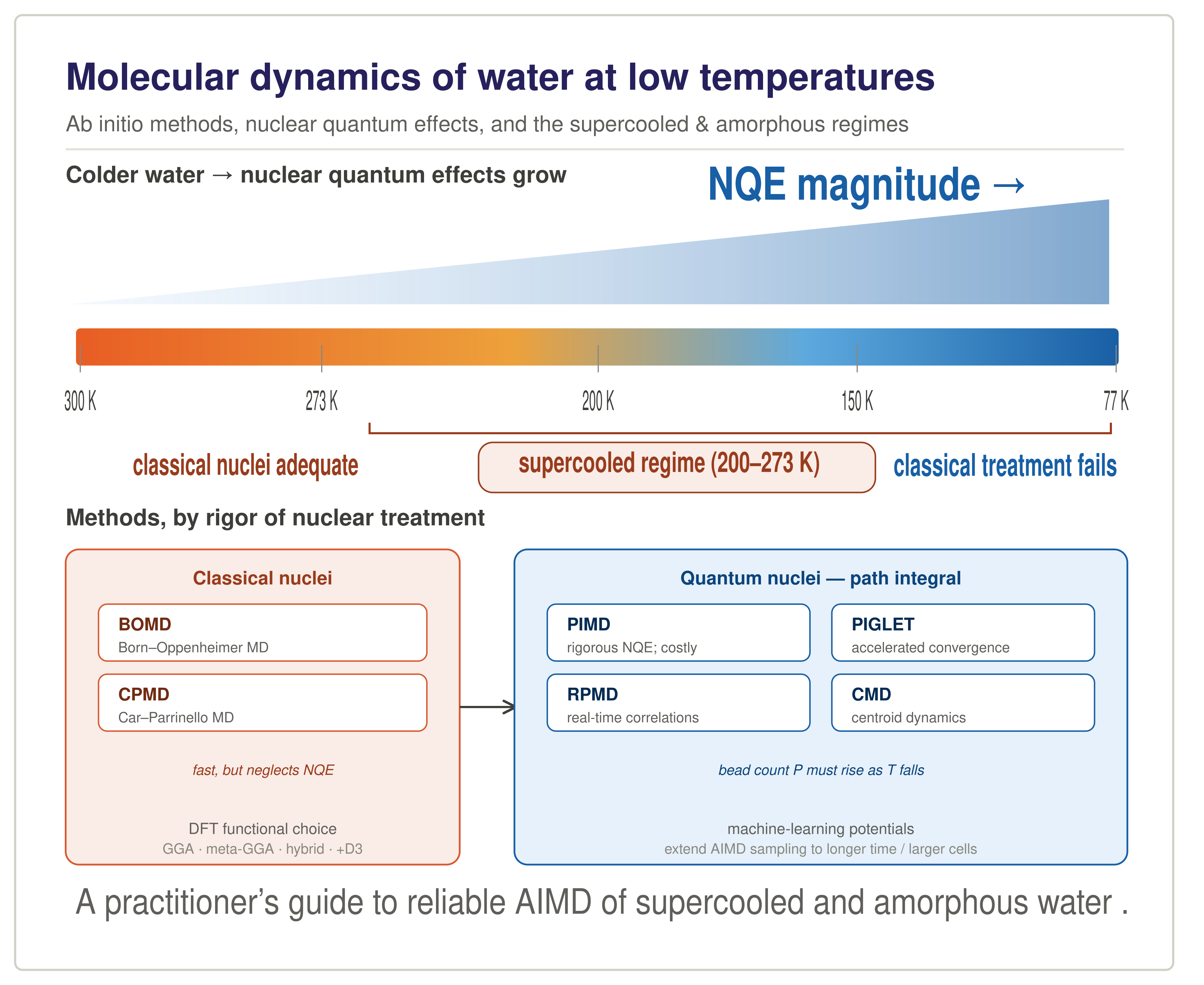
Water exhibits anomalous thermodynamic and structural behavior as it approaches and crosses below its melting point. Modelling this behaviour computationally remains challenging: as temperature decreases, nuclear quantum effects (NQE) become increasingly significant, sampling efficiency deteriorates dramatically, and the choice of computational method critically impacts the accuracy of predicted structural and dynamical properties. This review aims to provide practitioners with a comprehensive guide to performing reliable molecular dynamics simulations of water at low temperatures, with particular emphasis on the supercooled regime (200--273 K). We examine commonly used methods in ab initio molecular dynamics (AIMD) approaches, and critically evaluate strategies for incorporating nuclear quantum effects through path-integral molecular dynamics (PIMD), ring-polymer MD (RPMD), and centroid MD (CMD); below approximately 250 K the magnitude of nuclear quantum effects, and the sensitivity of structural and dynamical properties to them, grows to the point where classical treatment of the nuclei is no longer adequate. The known limitations of density functional approximations for water structure are assessed in the context of their interplay with NQE treatment, rather than in isolation. By discussing practical considerations, including sampling efficiency and the temperature scaling of path-integral bead counts, alongside the methods themselves, this review is intended to serve as a practical reference for reliable AIMD studies of supercooled water.
Keywords:
AIMD
; molecular dynamics
; supercooled water
; ice
; amorphous solid water
; nuclear quantum effects
; density functional theory
; path-integral molecular dynamics
; BOMD
1. Introduction
Water is arguably the most studied liquid in science, yet its behavior continues to reveal surprising complexity, particularly at low temperatures. The thermodynamic and transport properties of water deviate increasingly from simple-liquid behavior on cooling, with the deviations already apparent below the temperature of maximum density (∼277 K) and becoming increasingly dramatic upon supercooling below the equilibrium melting point (273 K) [1,2]. These anomalies (i.e.: density, isothermal compressibility and heat capacity changes) have motivated decades of theoretical and experimental investigation [3,4,5].
Understanding water behavior at low temperatures is not merely of academic interest. For example: supercooled water plays critical roles in atmospheric chemistry, where it exists metastably in clouds at temperatures as low as 235 K [6]. In biomedical sciences, supercooling preservation enables extended storage of organs, tissues, and cells for transplantation [7,8,9]. In food technology and material processing, controlling supercooled water states is essential for cryopreservation without ice crystal damage [10]. Amorphous solid water (ASW), formed by vapor deposition at cryogenic temperatures, is a widely form of water found in the universe, for instance, coating interstellar dust grains where it serves as a substrate for complex organic molecule (COM) formation [11,12,13,14]. In planetary science, water ice in various amorphous and crystalline forms is found on icy moons, comets, and Mars [15]. These diverse applications demand accurate theoretical descriptions, aimed to facilitate in silico experimentation, which has important adventages over wet lab experimentation as cost, time and reproducibility, among others.
Classical molecular dynamics (MD) simulations have provided valuable insights into water behavior, but they fundamentally cannot capture several phenomena critical to low-temperature systems. Chemical reactions, including the radical chemistry relevant to astrochemical environments, require explicit treatment of electronic structure. Moreover, the rigid non-polarizable classical water force fields neglect both electronic polarizability and nuclear quantum effects, which limits their accuracy for structural and thermodynamic properties of water at low temperatures [16].
Ab initio molecular dynamics (AIMD) simulations at low temperatures, face their own substantial challenges. First, the dynamics slow dramatically as temperature decreases, making adequate sampling increasingly difficult within accessible simulation timescales. Second, nuclear quantum effects (NQE), as zero-point energy, tunneling, and proton delocalization, become progressively more important as the thermal energy becomes comparable to vibrational zero-point energies. At 300 K, the ratio of hydrogen zero-point energy to thermal energy is about an order of magnitude, which increases when the temperature drops, [17] indicating that classical treatment of nuclei introduces significant systematic errors. Third, the accuracy of different density functionals for water remains a subject of ongoing investigation, with different approximations yielding qualitatively different predictions for structure and dynamics [18].
This review addresses these challenges systematically. We aim to provide practitioners with a comprehensive guide to performing reliable AIMD simulations of water in the 200–273 K temperature range. Section 2 briefly reviews the structural characteristics of water at low temperatures, including supercooled liquid water and amorphous ices, establishing the physical context and validation targets for simulations. Section 3 presents the principal AIMD approaches, from Born–Oppenheimer MD (BOMD) to path-integral MD (PIMD), and discusses how each addresses the specific challenges that water simulations face at ultra-low temperatures: slow dynamics and degraded sampling, the growing importance of nuclear quantum effects, and the sensitivity of structural and dynamical properties to the underlying potential energy surface. Section 4 addresses density functional selection for water. Section 5 addresses the central methodological challenge: nuclear quantum effects and their interplay with density functional selection.
2. Water Structure at Low Temperatures
First, it is essential to establish the physical phenomena that simulations must capture. This section reviews the structural evolution of water from ambient conditions through the supercooled regime to the glassy and crystalline states.
2.1. Supercooled Liquid Water
This metastable supercooled state has been accessed experimentally down to its homogeneous freezing limit of approximately 235 K in micrometre-sized samples [19], and to even lower temperatures using rapidly cooled nanodroplets [20] and ultrafast X-ray probing of evaporatively cooled microdroplets [21], the latter revealing metastable bulk liquid water down to 227 K.
The structure of supercooled water evolves continuously from ambient conditions, with an accelerating increase in ordering as temperature decreases. X-ray diffraction studies reveal that upon cooling, the first oxygen–oxygen radial distribution function (RDF) peak near 2.8 Å grows in height, while the running O–O coordination number exhibits a temperature-independent isosbestic point near 3.3 Å, and the second peak near 4.5 Å becomes increasingly pronounced below the compressibility-minimum temperature, reflecting enhanced tetrahedral coordination [22]. Measurements extending to 234.8 K show that intermediate-range correlations continue to strengthen upon supercooling, with the 4th and 5th peaks near 9 and 11 Å increasing in height and the 4th-peak position shifting to shorter distances [23]. At ambient conditions, water already exhibits nanometer-scale density fluctuations representing tetrahedral-like and hydrogen-bond-distorted structures [24]. These structural changes are often interpreted within a two-state framework, where water is viewed as a fluctuating mixture of locally tetrahedral, low-density liquid (LDL) and more disordered, high-density liquid (HDL) structural motifs [2]. More recent experiments reported observation of a liquid-liquid transition under pressure at 205 ± 10 K [25]. The temperature range between approximately 160 K and 232 K, often called the “no-man’s land”, has historically been inaccessible to bulk experiments due to rapid crystallization [21]. Solid water has been obtained at 77 K in different distinct glassy forms, from low-density amorphous ice (LDA) to high-density amorphous ice (HDA) [26,27]. However, our understanding of water’s structure below the homogeneous nucleation temperature, K, whether it reflects continuous structural evolution or a discrete liquid–liquid transition, continues to evolve, and computational simulations provide much of the structural insight into this experimentally challenging region.
2.2. Amorphous Ice
Amorphous ice phases are key benchmarks for low-temperature simulations. The principal forms relevant to this review are LDA, MDA, HDA, VHDA, and HGW.
2.2.1. Low-Density Amorphous Ice (LDA)
Formation temperature and conditions.
The low-density amorphous ices can be prepared by three routes that yield structurally similar forms of the same density (∼0.94 g cm−3): (i) vapour deposition of water onto a cold substrate, giving amorphous solid water (ASW) [28]; (ii) decompression (or controlled heating) of HDA, giving low-density amorphous ice (LDA), with the reversible HDA→LDA transition occurring at ∼135 K and ∼0.2 GPa [29]; and (iii) hyperquenching of micrometre-sized liquid droplets at cooling rates of order K/s, which vitrifies water to hyperquenched glassy water (structurally akin to LDA) [30,31].
In the interstellar medium, water is the most abundant ice species in grain mantles, built up by freeze-out of gas-phase species onto cold dust grains; this ice is predominantly amorphous [32].
Structure. The first peak of the oxygen–oxygen radial distribution function is located at Å [33,34]. LDA exhibits a locally tetrahedral hydrogen-bond network resembling ice but lacking long-range crystallographic order [33].
2.2.2. Medium-Density Amorphous Ice (MDA)
Density. MDA has a density of g cm−3 at 77 K and ambient pressure [37], falling within the density gap previously thought to be empty between LDA (∼0.94 g cm−3) and HDA (∼1.17 g cm−3) [26,38].
Formation temperature and conditions. MDA is produced by ball milling hexagonal ice (ice ) at 77 K using stainless-steel balls under cryogenic conditions [37].
Molecular dynamics simulations suggest that isobaric cooling at MPa can produce structurally similar amorphous states [39]. More recent simulations identify MDA as a shear-driven amorphous ice that can also be formed by shearing LDA or HDA at controlled shear rates [40].
Structure. The oxygen–oxygen pair-distribution function of MDA reveals a progressive collapse of the second coordination shell along the sequence ice → LDA → MDA → liquid water, placing MDA structurally closer to liquid water than to LDA [37]. Importantly, MDA is not a simple mixture of LDA and HDA; comparison of its diffraction pattern with other ice forms identifies it as a structurally unique material rather than a transition state or a mixture of existing forms [37].
Key remarks. MDA was first reported in 2023 by Rosu-Finsen et al. [37]. Its density near that of liquid water (∼1.00 g cm−3) raises the possibility that MDA may represent the true glassy state of liquid water, though this remains debated [37]. The discovery suggests a continuum of amorphous ice states rather than discrete phases separated by sharp density gaps.
2.2.3. High-Density Amorphous Ice (HDA)
Density. HDA has a density of approximately 1.17 g cm−3 at 77 K and ambient pressure [27]; the value reported for HDA obtained by compressing LDA at 77 K was ∼1.19 g cm−3 at zero pressure [27], while the originally reported HDA densities span ∼1.13–1.17 g cm−3 depending on the specific preparation protocol and degree of structural relaxation, with relaxed (expanded) HDA being ∼0.02 g cm−3 less dense than unannealed HDA [41,42].
Formation temperature and conditions. HDA is formed by: (i) pressure-induced amorphization of ice at 77 K under ∼1 GPa [26]; or (ii) compression of LDA at temperatures below ∼150 K, with the transition occurring at ∼0.6 GPa [27,43]. These transitions occur below the crystallization temperature of amorphous ice (∼150 K at ambient pressure) [44]. Importantly, unannealed HDA (uHDA) and equilibrated (expanded) HDA (eHDA) differ in their structural and thermal properties, reflecting the sensitivity of the amorphous state to thermal history [44,45].
Structure. The first O–O coordination shell is located at Å, with approximately 4 nearest oxygen neighbors in the first shell [34]. The structure features interpenetrating hydrogen-bond networks in which the second coordination shell collapses inward compared to the open tetrahedral arrangement of LDA [34]. Neutron diffraction studies of the five amorphous ices at 80 K and ambient pressure show that HDA is structurally distinct from both LDA and VHDA in its intermediate-range order [33].
Key remarks. HDA is approximately 20–25% denser than LDA [39]. Once formed, it can be recovered to ambient pressure at 77 K and stored for extended periods [46]. The apparently first-order LDA–HDA transition is widely interpreted as evidence supporting the liquid–liquid critical point hypothesis for water [1,47].
2.2.4. Very High-Density Amorphous Ice (VHDA)
Density. VHDA has a density of g cm−3 at 77 K and ambient pressure [38], approximately 9% higher than that of HDA. Values up to 1.26 g cm−3 have been reported depending on preparation pressure [48].
Formation temperature and conditions. VHDA is prepared by isobaric annealing of HDA at pressures of 1.1–1.9 GPa and temperatures of 165–177 K, followed by quenching to 77 K [38,48,49]. VHDA forms at pressures >0.8 GPa [48]. A stepwise transformation sequence LDA → HDA → VHDA (with HDA → VHDA at ∼0.95 GPa) has been observed at 125 K [43].
Structure. The first O–O coordination shell remains near ∼2.8 Å [38,50]. The Raman spectrum of VHDA differs clearly from HDA, with the hydrogen-bonded O–O distance increasing from 2.82 Å in HDA to 2.85 Å in VHDA [38]. Under pressure (∼2 GPa), the second coordination shell moves inward as interstitial neighbors are incorporated, distinguishing VHDA from HDA [51].
Key remarks. VHDA prepared at high pressures and temperatures (1.9 GPa, 175 K) represents the amorphous state of water at >0.7 GPa least affected by nanocrystalline remnants [49]. The activation barrier for the VHDA → HDA back-conversion is higher than for HDA → LDA [52]. The crystallization temperature of VHDA increases by up to 4 K when prepared at 1.9 GPa compared to 1.1 GPa, reflecting improved structural homogeneity [49].
2.2.5. Hyperquenched Glassy Water (HGW)
Density. HGW has a density of approximately 0.94 g cm−3, similar to LDA [53].
Formation temperature and conditions. HGW is produced by: (i) rapid spraying of micrometer-sized (∼5 m) water droplets into a cryogenic medium (e.g., liquid propane) at ∼80 K [31]; (ii) deposition of fine droplets onto a cold substrate at ≤80 K; or
(iii) cooling of water in capillary tubes (∼100 m diameter) with liquid helium at 4.2 K. The required cooling rates are on the order of – K/s [31].
Structure. HGW is structurally very similar to LDA and ASW, particularly after annealing [33]. It possesses a fully hydrogen-bonded, open tetrahedral network characteristic of low-density amorphous forms [34].
Key remarks. The glass transition temperature of HGW is K according to Johari, Hallbrucker, and Mayer [35,54]. However, this value is debated; Velikov, Borick, and Angell argued based on enthalpy relaxation scaling that K [55], while Kohl et al. presented DSC evidence supporting the 136 K assignment [56]. HGW is kinetically stable at 77 K and can be stored for years. Above , HGW behaves as an ultraviscous liquid before crystallizing near ∼150–154 K [56].
2.2.6. Summary of Amorphous Ice Properties
Table 1 provides a consolidated comparison of the principal amorphous ice phases.
2.3. Crystalline Ice Phases
For completeness and to provide validation targets for simulations, Table 2 summarizes the key crystalline ice phases relevant to low-temperature conditions at atmospheric and moderate pressures.
Ice (hexagonal ice) is the thermodynamically stable form of ice I at ambient pressure, whereas ice is metastable cubic ice [63]. In practice, what has often been reported as “cubic ice” is typically stacking-disordered ice , containing cubic sequences interlaced with hexagonal sequences [63], which results in variable density and .
X-ray diffraction measurements on freezing micron-sized water droplets show a droplet-size dependence, where smaller droplets freeze dominantly to cubic ice with stacking faults and larger droplets favour hexagonal ice [69].
Ice XI is the proton-ordered form of ice and is thermodynamically stable below ∼72 K (near ambient pressure) [70].
3. Ab Initio Molecular Dynamics Methods for Water
The theoretical description of atomic and molecular systems based on the Schrödinger equation emerged from early theoretical developments of electron and nuclear behavior. The Schrödinger equation molecular Hamiltonian comprises terms for nuclear kinetic energy, electronic kinetic energy, electron-nuclear attraction, electron-electron repulsion, and nuclear-nuclear repulsion. Solving this equation exactly for all but the simplest systems presents formidable computational challenges, given the exact mathematical form of the wavefunction is unknown. Thus, there are some common approximation methods that address the tradeoff between resource consumption and accuracy. This section presents the principal AIMD methods used for water simulations in cold regimes, emphasizing the fundamental origin of their limitations or adventages.
3.1. Born-Oppenheimer Molecular Dynamics (BOMD)
In BOMD, the electronic structure is converged self-consistently at each nuclear configuration, yielding forces from the ground-state energy surface [71]. Nuclei evolve according to Newton’s equations:
where and are the mass and position of nucleus I, and is the ground-state electronic energy.
The importance of these nuclear quantum effects can be quantified by the ratio of zero-point energy to thermal energy, . For the O–H stretching mode in water ( cm−1 [72]), the zero-point energy kcal mol−1, which already exceeds the thermal energy by an order of magnitude at room temperature [17]. As temperature decreases, this ratio grows further: at 200 K, kcal mol−1, making the ZPE approximately 13 times larger than the thermal energy available to the O–H coordinate.
BOMD performs a clean separation of electronic and nuclear timescales. With sufficiently tight self-consistent-field convergence at each step, it conserves the physical total energy, whereas CPMD conserves a different (extended-Lagrangian) constant of motion [71].
However, because the nuclei are propagated classically, BOMD is unable to compute zero-point energy or nuclear tunneling; errors grow as T decreases and the de Broglie thermal wavelength increases.
3.2. Car-Parrinello Molecular Dynamics (CPMD)
CPMD avoids explicit SCF convergence by treating electronic wavefunctions as dynamical variables with fictitious mass [75]:
where enforces orthonormality.
The method’s validity rests on adiabatic decoupling: the fictitious electronic frequency must greatly exceed nuclear frequencies , keeping electrons near the ground state. For water, two problems arise at low temperatures. The O-H stretching frequency (∼3600 cm−1) sets a high that constrains the choice of , requiring small timesteps of ∼0.12–0.24 fs [76,77]. As nuclear motion slows with decreasing T, maintaining the ratio becomes harder: small perturbations can transfer energy from electrons to nuclei, causing drift from the Born-Oppenheimer surface [77].
Advantages: Faster per step than BOMD; no SCF convergence at each step.
Limitations: Requires small timesteps; sensitive to the fictitious electronic mass tuning; potential energy drift for light atoms; shares BOMD’s classical-nuclei limitation.
Standard CPMD with classical nuclei is generally not recommended for water when nuclear quantum effects are required. Classical first-principles water is over-structured relative to experiment at room temperature, and including nuclear quantum effects softens the radial distribution functions and systematically improves agreement with experiment [78]. The underlying fictitious-mass sensitivity is also exacerbated in water specifically because of the high-frequency O–H stretching mode, which couples to the electronic dynamics and can cause drift from the Born–Oppenheimer surface [77]. For low-temperature water, both limitations remain: classical nuclei become a progressively worse approximation as the de Broglie wavelength of the proton grows — making methods with explicit NQEs (PIMD, PIGLET) the more appropriate choice.
3.3. Path-Integral Molecular Dynamics (PIMD)
Classical treatment of nuclei fails for light atoms at low temperatures. PIMD addresses this by exploiting the isomorphism between quantum statistical mechanics and classical mechanics of ring polymers [79,80]: each quantum particle of mass M is represented by P classical “beads” connected by harmonic springs, with spring constant , where . The temperature dependence of is the central feature: at low T the springs weaken (quadratically), allowing the ring polymer to “open” and directly represent the growing thermal de Broglie wavelength of the quantum particle.
Convergence to the quantum limit requires , where is the highest physical frequency in the system [17]. For water, cm−1.
For water at room temperature, replicas are typically required to converge structural properties [17]; the requirement grows roughly as for fixed , making low-temperature PIMD considerably more expensive.
Since standard PIMD evaluates forces independently for each bead, computational cost scales linearly with P [17]. Note that converging O–H structural properties requires at least at 300 K [17]; the scaling implies –64 at 150–200 K, placing standard ab initio PIMD tens to hundreds of times more expensive than classical BOMD, which is often prohibitive for production runs.
3.4. Accelerated Path-Integral Methods
Several approaches reduce PIMD’s computational burden while preserving essential quantum effects:
Ring-polymer contraction (RPC) exploits the observation that the physical potential varies more slowly than the inter-bead springs. Expensive DFT forces can be evaluated on a contracted ring ( beads), with projection back to the full ring [81]. This is particularly effective when a reference potential can absorb the rapidly varying forces, leaving a smoothly varying remainder for the contracted ring [17].
PI-GLE (Ceriotti, Manolopoulos, Parrinello) [82] employs a generalized Langevin equation thermostat with colored noise to accelerate the convergence of path integral molecular dynamics in anharmonic systems exhibiting both zero-point energy and tunnelling effects. Unlike white noise, colored noise mimics the quantum fluctuation spectrum, designed so that a P-replica PIMD simulation converges structural observables in the harmonic limit for any P. PIGLET [83] extends this scheme with additional constraints on the noise spectrum, so that the quantum kinetic energy estimator also converges in the harmonic limit at small P. Together, these approaches achieve converged NQEs with as few as ∼6 beads at 300 K for liquid water [83].
The key insight underlying both methods is that quantum statistics require energy distributed according to per mode rather than the classical equipartition value ; the GLE thermostat enforces this distribution while reducing the number of beads required for convergence. Both methods are implemented in i-PI [84], which interfaces with CP2K and other electronic-structure codes.
3.5. Machine-Learning Interatomic Potentials
Machine-learning interatomic potentials (MLPs), including neural-network potentials and kernel-based methods such as Gaussian Approximation Potentials, are trained on a database of ab initio (typically DFT) energies and forces, and then used as a drop-in replacement for the underlying potential energy surface during MD [85,86]. Once trained, force evaluations cost a small fraction of a DFT step. They can be combined with BOMD, PIMD, PIGLET, RPMD, or CMD, and the speedup applies in each case. In the path-integral context in particular, the P-fold overhead of bead sampling becomes affordable, and nanosecond-scale path-integral trajectories of condensed-phase water at near-DFT accuracy are now feasible [87].
A comprehensive review of MLPs for water is beyond the scope of this work; we refer the reader to a recent dedicated review on neural-network potentials [88], and note that data-driven quantum simulations have recently reproduced the water phase diagram at near-first-principles accuracy [89]. We note one caveat directly relevant to the present review: the great majority of MLPs for water reported to date have been trained and validated on reference data sampled at or near ambient conditions. Their transferability to the deeply supercooled regime (200–250 K), and especially to the amorphous ice phases discussed in Section 2.2, is not guaranteed and remains an active research question. Studies that use MLPs for low-temperature water should therefore include explicit validation against ab initio reference points at the temperatures and densities of interest, rather than relying on extrapolation from ambient-condition training sets.
3.6. Comparison of AIMD Methods
Table 3 provides a comprehensive comparison of AIMD methods for water simulations.
General remarks for method selection:
- Method selection depends on the target observable, the required accuracy, and the temperature regime, rather than on a single criterion. Table 3 summarizes the trade-offs. Broadly: classical-nuclei AIMD (BOMD, or CPMD with a small fictitious mass) is appropriate when NQE corrections to the target property are smaller than other modeling errors; path-integral methods (PIMD, PIGLET) are needed when quantum statistics of the nuclei matter, with the number of beads P growing as T decreases; and approximate quantum-dynamics methods (RPMD, CMD/QCMD, instanton) are needed when real-time correlation functions, vibrational spectra, or rate constants are required. The boundaries between these regimes are not sharp and should be assessed against benchmarks for the specific property of interest.
4. Density Functional Selection for Water
The functional choice is perhaps the most consequential decision in DFT-based AIMD of water. Water presents a stringent test for density functionals because accurate simulation requires simultaneous description of:
- Intramolecular covalent bonding (O-H stretching, H-O-H bending)
- Intermolecular hydrogen bonding (electrostatic + charge transfer)
- London dispersion interactions
- Many-body polarization effects
Different classes of functionals handle these interactions with varying fidelity, and errors in any component propagate into structural and dynamical predictions [18]. Below we discuss these nuances family by family, presenting representative members of each class, including both widely-used functionals and those that have performed comparatively well in benchmark studies of liquid water and ice. We note an important caveat: most systematic benchmarks of these functionals have been carried out at or near ambient conditions, including the broad surveys of Gillan et al. [18] and the more recent force-based benchmark of 50+ functionals by Cui [95]. Direct DFT-AIMD validation of any functional in the supercooled regime (200–250 K) and for the amorphous ice phases of Section 2.2 remains sparse. Most of what is known about low-temperature water at the DFT level comes indirectly through machine-learning potentials trained on DFT reference data [87,96,97,98], which then enable the much longer trajectories needed to probe supercooled and amorphous states.
4.1. Generalized Gradient Approximation (GGA) Functionals
GGA functionals are computationally efficient but suffer from well-documented limitations for water:
BLYP [99,100]: Without dispersion correction, BLYP over-structures liquid water and underestimates its diffusivity (i.e., the dynamics becomes too sluggish) [101,102]; the density of the liquid is also significantly under-predicted [102]. Adding an empirical Grimme dispersion correction (BLYP-D in the original Schmidt et al. study, equivalent to modern BLYP-D3 in current practice) significantly improves the predicted density and brings the O–O radial distribution function into close agreement with experiment [102]. The resulting BLYP-D3 potential energy surface is comparatively “soft,” and several authors have argued that this softness partially compensates for the missing nuclear quantum delocalization in classical-nuclei simulations [18]. Performance of BLYP-D3 in the supercooled regime (200–250 K) is sparse. However some structural features (ie. g(r)O–O) are covered in the 225–350 K range in Tatini2015.
Advantages: Fast computation; soft PES partially compensates for missing NQE; good for equilibration.
Disadvantages: Bare BLYP underbinds the water dimer (4.18 kcal mol−1 vs 5.44 kcal mol−1 experimental) [103] and produces an overstructured liquid with too slow diffusion ( below experiment) [103,104]. Adding D3 brings density and the O–O RDF close to experiment [102], but barrier heights remain unreliable: the GMTKN55 BH76 WTMAD-1 is 5.19 kcal mol−1 for BLYP and 5.53 kcal mol−1 for BLYP-D3(BJ), reflecting an underlying self-interaction error that dispersion correction does not address [105].
PBE [106]: PBE tends to over-structure radial distribution functions of water even at ambient conditions, predicting too many hydrogen bonds and underestimating diffusivity, with respect to experiments [103]. PBE beneffits from adding dispersion (PBE-D3) improving structural parameters. However, dispersion correction has limited effect on bulk water structure because PBE already overbinds molecules [18].
Advantages: Well-validated; widely available; reasonable lattice constants for ice [103].
Disadvantages: Over-structures liquid water, an artifact not fully removed by adding dispersion corrections [101,103]; poor dynamics in the supercooled regime[107]; severely overestimates the melting point of ice [108], equivalent to over-stabilizing ice relative to liquid.
revPBE-D3 [109,110]: revPBE without dispersion correction performs poorly for condensed-phase water, but combined with Grimme’s D3 dispersion correction it has been reported to describe ambient liquid water (298 K, 1 atm) remarkably well in classical AIMD, with equilibrium density, , self-diffusivity, IR spectrum, and dipole moment in reasonable agreement with experiment [111]. This performance partly reflects a cancellation between intrinsic functional error and the neglect of nuclear quantum effects in classical-nuclei trajectories [111]. Direct validation in the supercooled regime is sparse: in the ab initio benchmark of Herrero et al. down to ∼248 K, the SCAN functional was found to perform better, while revPBE-D3 was identified as a plausible alternative that describe the temperature evolution of the shear viscosity and self-diffusion coefficient of liquid waterwith good performance, but was not itself tested across the full supercooled range [107]. Consequently, applicability of revPBE-D3 to the 200–273 K regime should be regarded as inferred from ambient-temperature benchmarks rather than directly validated.

Table 4.
Summary of GGA functional performance for water at ambient conditions (∼300 K, 1 atm). Density and errors are deviations from experimental liquid-water values, computed as (functional value − experimental value) using raw simulation data tabulated in the cited primary references. The experimental reference values g cm−3 (room temperature, 1 atm) and Å [112] are also taken from the same primary references. The barrier error is the mean absolute deviation from CCSD(T)/CBS reference values on the gas-phase BH76 subset of GMTKN55 [105], taken directly from the supporting information of that work, and is reported as a generic indicator of transition-state energetics, not a water-specific benchmark. revPBE values are from simulations performed at 330 K (rather than 300 K), as reported in Ref. [113] to compensate for revPBE’s over-structuring tendency, and is therefore not directly comparable to the other rows. No directly comparable benchmark data was found for any of these functionals in the supercooled regime (200–273 K).
Table 4.
Summary of GGA functional performance for water at ambient conditions (∼300 K, 1 atm). Density and errors are deviations from experimental liquid-water values, computed as (functional value − experimental value) using raw simulation data tabulated in the cited primary references. The experimental reference values g cm−3 (room temperature, 1 atm) and Å [112] are also taken from the same primary references. The barrier error is the mean absolute deviation from CCSD(T)/CBS reference values on the gas-phase BH76 subset of GMTKN55 [105], taken directly from the supporting information of that work, and is reported as a generic indicator of transition-state energetics, not a water-specific benchmark. revPBE values are from simulations performed at 330 K (rather than 300 K), as reported in Ref. [113] to compensate for revPBE’s over-structuring tendency, and is therefore not directly comparable to the other rows. No directly comparable benchmark data was found for any of these functionals in the supercooled regime (200–273 K).
| Functional |
Density Error (%) |
Error (Å) |
Barrier Error (BH76) (kcal mol−1) |
| BLYP | [114] | [114] | [105] |
| BLYP-D3 | [114] | [114] | [105] |
| PBE | [102] | [103] | [105] |
| PBE-D3 | [114] | [114] | [105] |
| revPBEa | [113] | [113] | [105] |
| revPBE-D3 [109,110] | [115] | [115] | [105] |
a
4.2. Meta-GGA Functionals
Meta-GGA functionals incorporate the kinetic energy density , providing additional flexibility:
SCAN [116]: The strongly constrained and appropriately normed (SCAN) functional satisfies all 17 known exact constraints for a semi-local functional. For water, SCAN captures the density difference between liquid water and ice at ambient conditions and reproduces many structural, electronic, and dynamic properties of liquid water without empirical dispersion corrections [117], and correctly predicts ice as more stable than ice along with reasonable melting properties of both polymorphs [118]. However, SCAN overestimates the liquid water density by approximately 5% relative to experiment [117] and can exhibit numerical grid sensitivity in some implementations [119,120].
Advantages: No empirical parameters; good ice energetics including correct / stability ordering; captures intermediate-range dispersion.
Disadvantages: Over-dense liquid (∼5%); grid sensitivity; computational overhead (1.5–2× GGA); can be unstable in some codes.
r2SCAN [120]: A regularized version of SCAN with improved numerical stability.
For water, r2SCAN-driven AIMD reproduces the structure of bulk liquid water at ambient density when simulations are run at an elevated temperature of 350 K, similar to the compensation required for SCAN, which exhibits excessive structuring at 300 K and an augmented first solvation shell at 330 K [121]. The first O–O peak position of r2SCAN (2.865 Å) sits slightly above the experimental value (2.801 Å), indicating mild residual over-structuring [121]. Furness et al. report that r2SCAN converges with fewer iterations than SCAN [120].
Advantages: Improved numerical convergence over SCAN [120]; comparable structural accuracy for bulk liquid water at ambient conditions [121].
Disadvantages: Inherits SCAN’s need for an elevated simulation temperature (∼350 K) to match the 300 K experimental RDF [121]; mild over-structuring of the first O–O peak relative to experiment [121].
DC-SCAN (Density-corrected SCAN): Applies a Hartree–Fock density correction scheme to SCAN, minimizing density-driven errors and elevating the accuracy of the SCAN functional to that of coupled-cluster theory for water clusters and interaction energies [122].
Advantages: Reaches near-coupled-cluster accuracy for water cluster energetics; reduces SCAN’s overbinding/over-structuring tendencies; provides a reliable reference for parameterizing many-body and machine-learned potentials.
4.3. Hybrid Functionals
Hybrid functionals include a fraction of exact (Hartree-Fock) exchange, improving descriptions of charge transfer and reducing self-interaction error [123].
In the context of liquid water, hybrid functionals combined with nuclear quantum effects (NQEs) have been shown to provide a markedly improved description of hydrogen bonding, with revPBE0-D3 + PIMD identified as one of the few approaches that closely agrees with experiment [124].
PBE0 [125]: With 25% exact exchange and, when paired with D3 dispersion correction (PBE0-D3), this functional provides excellent barrier heights for reactions [126,127] and reliable magnetic properties [128]. Under classical nuclei, PBE0-D3 tends to over-structure liquid water [129].
The computational cost is substantially higher than GGA due to the evaluation of exact exchange (commonly an order of magnitude or more in conventional Gaussian or plane-wave AIMD implementations), although schemes like ADMM can reduce this overhead by roughly a factor of 20 [130].
Advantages: Excellent barrier heights (MAD ∼1–2 kcal mol−1 on representative benchmarks) [127]; reliable magnetic properties [128]; reduced self-interaction error [123]; improved hydrogen-bond description, particularly when combined with NQEs [131].
Disadvantages: Substantial cost increase over GGAs [130]; tends to over-structure water under classical nuclei [129]; requires dispersion correction (e.g., D3 [110]) for condensed phases [129].
revPBE0: Combines the exchange of revPBE with 25% exact exchange. This functional has been shown to accurately reproduce the structure, dynamics, and vibrational spectroscopy of bulk liquid water when combined with path-integral simulations and D3 dispersion. [87,124,132], and is one of the few approaches that yields quantitative agreement with experiment for the O–O radial distribution function, self-diffusion coefficient, and full IR and Raman spectra at ambient conditions [124,132].
Advantages: Among the best-performing functionals for bulk liquid water when combined with NQEs, capturing the O–O RDF, diffusion, and IR/Raman spectra in close agreement with experiment [87,124,132]; balanced description of covalent bonding and hydrogen bonding such that competing nuclear quantum effects on the hydrogen bond cancel correctly [124].
Disadvantages: Substantial cost overhead from the evaluation of exact exchange in periodic AIMD, although acceleration schemes such as the auxiliary density matrix method (ADMM) significantly reduce this cost [130]; NQE treatment essential for quantitative agreement of dynamics and vibrational spectra [124,132].
B97X-V [133]: A range-separated hybrid GGA with non-local correlation functional VV10, designed against a broad training set covering thermochemistry, kinetics, and non-covalent interactions. Its meta-GGA counterpart B97M-V [134] extends this design to the meta-GGA rung. On benchmark sets of small water clusters with coupled-cluster reference binding energies, B97X-V and B97M-V have been reported to give the smallest errors among the DFT functionals tested in that set [135]. A closely related meta-GGA, B97M-rV (B97M-V with the rVV10 non-local correlation [136]), gives bulk liquid water structure, diffusion, and IR spectroscopy of comparable accuracy to the much more expensive hybrid revPBE0-D3 when combined with path-integral simulations [132], and is therefore an attractive meta-GGA-level alternative to hybrid functional for bulk water.
Advantages: Smallest binding-energy errors among DFT functionals tested on water-cluster benchmarks against coupled-cluster references [135]; built-in VV10 non-local correlation, so no separate dispersion correction is required [133,137]; the related meta-GGA B97M-rV reaches near-hybrid accuracy for bulk water at meta-GGA cost [132].
Disadvantages: Substantial cost relative to GGA functionals, from range-separated exact exchange combined with VV10 non-local correlation evaluation; less commonly used in condensed-phase AIMD of liquid water than global hybrids such as PBE0 and revPBE0.
4.4. Dispersion Corrections
Standard DFT functionals miss long-range dispersion interactions, which contribute significantly to ice cohesion (see [138,139] ). Common corrections include:
- D4 [141] Improved atom-pairwise dispersion with charge-dependent coefficients.
- VV10 [137]: Vydrov and Van Voorhis non-local correlation functional that captures dispersion from the electron density alone. More physically motivated than atom-pairwise schemes, but computationally more demanding due to the six-dimensional double integral over the density.
For water simulations, D3(BJ) is chosen as the default method due to its extensive validation, low computational overhead, and availability in all major codes.
5. Nuclear Quantum Effects: The Challenge Below 250 K
5.1. Physical Origin of Nuclear Quantum Effects
Because electrons move much faster than nuclei due to their significantly smaller mass, the Schrödinger equation is commonly simplified using the Born-Oppenheimer approximation. This approximation underlies the most widely used methods for molecular dynamics, including BOMD, CPMD, and standard DFT-based approaches. According to Born-Oppenheimer, the electronic wavefunction is solved quantum mechanically at fixed nuclear positions, separating the electronic and nuclear degrees of freedom and the nuclei movement. This generates a potential energy surface on which nuclei evolve. A further approximation (treating nuclei as classical point particles obeying Newton’s equations) is applied in standard MD methods. This classical treatment of nuclei provides accurate results with reasonable computational cost under most conditions but inherently neglects nuclear quantum effects (NQE) such as zero-point energy (the minimum energy a particle possesses even at 0 K) and quantum tunneling, where a nucleus can traverse a potential energy barrier even when its kinetic energy is classically insufficient. For most systems at ambient conditions, neglecting NQE introduces minimal error and is therefore an acceptable approximation [71].
The fundamental limitation for low-temperature water lies in treating nuclei as classical point particles obeying Newton’s equations. This approximation neglects zero-point energy, quantization of vibrational energy levels, and tunneling. The importance of these nuclear quantum effects can be quantified by the ratio of zero-point energy to thermal energy, . For the O–H stretching mode in water ( cm−1 [72]), the zero-point energy kcal mol−1, which already exceeds the thermal energy by 9 times at room temperature [17]. As temperature decreases, this ratio grows further: at 200 K, kcal mol−1, making the ZPE approximately 13 times larger than the thermal energy available to the O–H coordinate.
Consequently, Eq. (1) introduces systematic errors that grow progressively with decreasing temperature, as the classical treatment cannot account for the proton delocalization, enhanced hydrogen-bond fluctuations, and tunneling contributions that become increasingly dominant in the supercooled regime [17,131].
The three principal phenomena of NQE are:
1. Zero-point energy (ZPE): Quantum mechanics mandates that a particle confined in a potential well possesses a minimum energy even at absolute zero temperature, where is the vibrational frequency. For the O-H stretching mode in water, the estimated ZPE 5.1 kcal mol−1 is comparable to the hydrogen bond strength itself (∼5 kcal mol−1). This ZPE causes hydrogen atoms to be more delocalized than classical mechanics predicts at all temperatures, effectively “swelling” the proton distribution perpendicular to the bond direction. This delocalization persists at ambient conditions but becomes increasingly dominant as temperature decreases and the ratio ZPE/ grows.
2. Quantum tunneling: Nuclei can traverse potential energy barriers even when their kinetic energy is classically insufficient to surmount them. For light nuclei such as hydrogen, this effect is particularly pronounced: the tunneling probability depends exponentially on both the barrier width and the particle mass, and the low mass of the proton makes hydrogen transfer reactions especially susceptible.
3. Exchange effects: In principle, identical nuclei should obey quantum exchange statistics (Bose-Einstein or Fermi-Dirac). However, in molecular water and ice, protons are localized in deep covalent potential wells (∼1 eV), which exponentially suppresses the inter-molecular wavefunction overlap required for exchange. In standard path integral simulations of water, nuclei are treated as distinguishable particles [17], and this approximation is considered valid at all temperatures relevant to condensed-phase water, in contrast to weakly bound systems such as superfluid helium where exchange effects dominate [142]. Bosonic-exchange path integral methods do exist [143] but are unnecessary in this regime. Exchange effects are therefore not considered further in this review.
Competing quantum effects in hydrogen bonding. NQE do not simply weaken or strengthen hydrogen bonds; they produce competing effects [131,144]:
- Intramolecular ZPE (O-H stretch): Causes proton delocalization perpendicular to the bond, weakening the hydrogen bond by increasing the average O···H distance.
- Intermolecular ZPE (O···O stretch): Causes delocalization along the hydrogen bond axis, which can strengthen hydrogen bonds by allowing closer O-O approach in the delocalized wavefunction.
The balance between these competing effects is functional-dependent and temperature-dependent.
5.2. Magnitude of NQE Versus Temperature
The ratio of zero-point energy (ZPE) to thermal energy provides a quantitative measure of NQE importance:
Table 5.
Comparison of thermal energy and H-atom zero-point energy in water. The ZPE is computed from the O-H stretching frequency (∼3600 cm−1, corresponding to ∼10.3 kcal mol−1 for two O-H bonds, or ∼5.1 kcal mol−1 per bond).
Table 5.
Comparison of thermal energy and H-atom zero-point energy in water. The ZPE is computed from the O-H stretching frequency (∼3600 cm−1, corresponding to ∼10.3 kcal mol−1 for two O-H bonds, or ∼5.1 kcal mol−1 per bond).
| T (K) | (kcal mol−1) | ZPE(OH)/() | (Å) |
|---|---|---|---|
| 300 | 0.60 | ∼8.5 | 1.0 |
| 250 | 0.50 | ∼10 | 1.1 |
| 200 | 0.40 | ∼13 | 1.2 |
| 150 | 0.30 | ∼17 | 1.4 |
| 77 | 0.15 | ∼34 | 2.0 |
Across the entire supercooled and glassy range the zero-point energy of the O–H stretch exceeds the thermal energy by roughly an order of magnitude or more, so classical treatment of nuclei introduces qualitative errors in properties sensitive to hydrogen motion. The thermal de Broglie wavelength approaching or exceeding the O–H bond length (∼1 Å) signals that protons cannot be treated as localized classical particles.
5.3. Isotope Substitution as an Experimental Probe of NQE
Nuclear quantum effects manifest experimentally as isotope effects: replacing H by D (or 16O by 18O) alters the zero-point energy and hence the measured structure, dynamics, and thermodynamics, which makes the H2O/D2O comparison the principal experimental route for validating quantum-nuclei simulations [131]. The competing intra- and intermolecular contributions introduced above (Section 5.1) are central to interpreting these data. Although the underlying changes are sizeable, with the O–H covalent bond roughly 3% longer than O–D and the associated hydrogen bond about 4% shorter, the opposing shifts largely offset, so that the net geometric isotope effect on the O–H distance in liquid water and ice is only ∼0.001 Å: the competing quantum effects almost exactly cancel under these conditions [131]. Water’s isotope effects consequently span a wide range across properties, from very large to almost negligible depending on the property and the thermodynamic conditions [17], a dichotomy that the competing-quantum-effects principle rationalises. Because reproducing this balance requires an accurate description of a broad region of the potential energy surface, isotope-resolved observables (geometries, proton kinetic energies, and fractionation ratios) provide a stringent simultaneous test of both the electronic-structure method and the nuclear treatment [131].
5.4. Structural Consequences of NQE
Classical nuclei predictions diverge from quantum reality in several ways at low temperature [131,145]:
Density trends: Classical MD predicts monotonically increasing density upon cooling, whereas PIMD reveals a density maximum in low-density amorphous ice that is absent in the classical treatment [145]. This qualitative difference arises because ZPE-induced volume expansion counteracts thermal contraction at low T.
Hydrogen bond geometry: Classical simulations tend to produce overly structured, overly linear O–H···O hydrogen bonds. NQE-induced proton delocalization perpendicular to the O–H bond direction softens the intermolecular structure and yields more bent hydrogen bonds, broadening the O–O radial distribution function relative to the classical result [78,146].
Radial distribution functions: First-neighbor peaks in and are sharper in classical simulations than with NQE. Including quantum effects broadens these peaks toward experimental values [78,146].
Vibrational spectra: The O–H stretching frequency is red-shifted in condensed phases due to hydrogen bonding. NQE further modulate these shifts through anharmonic coupling and Fermi resonances [124].
6. Conclusions and Outlook
Simulating water between 200 and 273 K confronts three coupled challenges: sampling degrades as the dynamics slow, nuclear quantum effects (NQE) grow from a correction into a dominant contribution, and structural and dynamical observables remain sensitive to the underlying potential energy surface. These cannot be treated in isolation; a reliable low-temperature simulation matches the rigour of the nuclear treatment to the rigour of the electronic structure. For a newcomer, this reduces to a small number of practical decisions.
Choosing the propagation scheme. BOMD on a well-converged Born–Oppenheimer surface is the natural baseline whenever NQE are smaller than the other modelling errors [17,71]. CPMD [75] is competitive in cost per step, but its fictitious-mass dependence and the difficulty of maintaining adiabaticity in the presence of the high O–H stretching frequency make it the weaker choice when low-temperature accuracy is the goal [77]. When the quantum statistics of the nuclei must be captured, imaginary-time path-integral methods (PIMD [79,80], accelerated through PIGLET [82,83] or ring-polymer contraction [81]) are the appropriate tools, with the bead number P scaling as and therefore rising as temperature falls. Approximate real-time methods (RPMD [90,91]; CMD and its quasi-centroid variant [93,94]) remain the route to vibrational spectra and reaction rates, but each carries characteristic artefacts (spurious resonances in RPMD and curvature-induced frequency shifts in CMD) that are amplified as T decreases [91,92].
Choosing the functional. Electronic-structure accuracy cannot be decoupled from the nuclear treatment. Dispersion-corrected GGAs such as revPBE-D3 owe part of their good ambient performance to a cancellation between the functional’s intrinsic error and the neglect of NQE in classical-nuclei trajectories [111]; this is a fortuitous balance, not evidence of accuracy at 200 K. Meta-GGAs (SCAN, r2SCAN) describe intermediate-range dispersion and ice-polymorph energetics well [116,117,118,120], but reproduce ambient liquid structure only when simulated at elevated temperature [121], a workaround that mimics the missing NQE rather than supplying them. Hybrid functionals combined with explicit path integrals (e.g. revPBE0-D3 + PIMD) are among the few combinations that quantitatively reproduce both structure and spectroscopy [124,131,132], at a cost that has historically restricted them to short trajectories on small cells.
Why the regime is special. Below roughly 250 K, NQE shift from a correction to an organizing principle: the ratio of O–H zero-point energy to thermal energy grows well past unity, and properties as basic as the temperature of maximum density of low-density amorphous ice cannot be recovered with classical nuclei [17,145]. Choices that look conservative at ambient conditions, such as classical nuclei or a GGA selected on room-temperature benchmarks, therefore become uncontrolled here. Standard path-integral simulations treat protons as distinguishable particles [17], an approximation kept robust for condensed water by the deep covalent localization of the O–H bond, in contrast to systems such as superfluid helium where exchange dominates [142]; bosonic-exchange path-integral methods exist [143] but are unnecessary in this regime.
Where the field is heading. A consequential recent development is the maturation of machine-learning interatomic potentials (MLPs) trained on high-level ab initio reference data [85,86,88,89]. By lowering the per-step cost of a force evaluation by orders of magnitude, MLPs make nanosecond-scale path-integral trajectories feasible, at the accuracy of their underlying ab initio reference, on the system sizes required for nucleation, phase-equilibrium, and amorphous-ice studies [87,96,97,98], and they are now the route by which most quantitative low-temperature results reach the literature. The principal caveat is transferability: an MLP trained on ambient data is not guaranteed to hold at 200–250 K or in amorphous phases, so explicit ab initio validation at the target conditions remains essential. Several gaps follow directly: direct DFT-AIMD benchmarks in the supercooled regime are sparse, functional rankings still rest largely on ambient data, and approximate quantum-dynamics methods need further development below 200 K. We expect MLP-driven, path-integral simulations, trained on hybrid or density-corrected reference data and validated against the structural targets of Section 2.2, to become the practical workflow of the coming decade.
Why it matters. Supercooled and amorphous water are the relevant phases for ice nucleation in mixed-phase clouds and in freezing atmospheric droplets [69,147], for the survival of organs under sub-zero preservation [7,8], for nucleation control in cryopreservation and food processing [10], and for the chemistry on amorphous-solid-water grain mantles in dense interstellar clouds that builds complex organic and prebiotic molecules [11,12,13,14]; amorphous and crystalline ices likewise dominate the surfaces of icy moons, comets, and Mars [15]. In each setting, prediction demands quantitative agreement with experiment at temperatures where NQE are non-negligible and direct measurement is fragmented. The convergence outlined above, path-integral sampling driven by machine-learning potentials trained on hybrid-functional reference data, brings these problems within reach of routine simulation at the system sizes and trajectory lengths the underlying physics demands.
Author Contributions
Conceptualization, F.C.; writing—original draft preparation, F.C.; writing—review and editing, F.C. and K.G.; supervision, J.B. All authors have read and agreed to the published version of the manuscript.
Funding
This research was supported by grant 0311/SBAD/0781 from Poznan University of Technology. Selected computational results reported herein were independently verified at the Poznań Supercomputing and Networking Centre.
Data Availability Statement
Not applicable.
Acknowledgments
The infrastructure of the European Centre for Bioinformatics and Genomics affiliated with the Poznan University of Technology (Poznan, Poland) was used in this work. Computations to corroborate some of the information presented were performed at the Poznan Supercomputing and Networking Centre.
Conflicts of Interest
The authors declare no conflicts of interest.
Abbreviations
The following abbreviations are used in this manuscript:
| AIMD | Ab initio molecular dynamics |
| ASW | Amorphous solid water |
| BOMD | Born–Oppenheimer molecular dynamics |
| CMD | Centroid molecular dynamics |
| COM | Complex organic molecule |
| CPMD | Car–Parrinello molecular dynamics |
| DFT | Density functional theory |
| GGA | Generalized gradient approximation |
| GPW | Gaussian and augmented plane waves |
| HDA | High-density amorphous ice |
| HDL | High-density liquid |
| HGW | Hyperquenched glassy water |
| LDA | Low-density amorphous ice |
| LDL | Low-density liquid |
| MD | Molecular dynamics |
| MDA | Medium-density amorphous ice |
| NQE | Nuclear quantum effects |
| PIMD | Path-integral molecular dynamics |
| RDF | Radial distribution function |
| RPMD | Ring-polymer molecular dynamics |
| VHDA | Very high-density amorphous ice |
| ZPE | Zero-point energy |
References
- Debenedetti, P. G.; Stanley, H. E. Supercooled and Glassy Water. Phys. Today 2003, 56(6), 40–46. [CrossRef]
- Nilsson, A.; Pettersson, L. G. M. The Structural Origin of Anomalous Properties of Liquid Water. Nat. Commun. 2015, 6, 8998. [CrossRef]
- Angell, C. A. Supercooled Water. Annu. Rev. Phys. Chem. 1983, 34, 593–630. [CrossRef]
- Speedy, R. J.; Angell, C. A. Isothermal Compressibility of Supercooled Water and Evidence for a Thermodynamic Singularity at −45 °C. J. Chem. Phys. 1976, 65, 851–858. [CrossRef]
- Stanley, H. E.; Buldyrev, S. V.; Canpolat, M.; Mishima, O.; Sadr-Lahijany, M. R.; Scala, A.; Starr, F. W. The Puzzling Behavior of Water at Very Low Temperature. Phys. Chem. Chem. Phys. 2000, 2, 1551–1558. [CrossRef]
- Murray, B. J.; O’Sullivan, D.; Atkinson, J. D.; Webb, M. E. Ice Nucleation by Particles Immersed in Supercooled Cloud Droplets. Chem. Soc. Rev. 2012, 41, 6519–6554. [CrossRef]
- Berendsen, T. A.; Bruinsma, B. G.; Puts, C. F.; Saeidi, N.; Usta, O. B.; Uygun, B. E.; Izamis, M.-L.; Toner, M.; Yarmush, M. L.; Uygun, K. Supercooling Enables Long-Term Transplantation Survival Following 4 Days of Liver Preservation. Nat. Med. 2014, 20, 790–793. [CrossRef]
- de Vries, R. J.; Tessier, S. N.; Banik, P. D.; Nagpal, S.; Cronin, S. E. J.; Ozer, S.; Hafiz, E. O. A.; van Gulik, T. M.; Yarmush, M. L.; Markmann, J. F.; et al. Supercooling Extends Preservation Time of Human Livers. Nat. Biotechnol. 2019, 37, 1131–1136. [CrossRef]
- Usta, O. B.; Kim, Y.; Ozer, S.; Bruinsma, B. G.; Lee, J.; Demir, E.; Berendsen, T. A.; Puts, C. F.; Izamis, M.-L.; Uygun, K.; Uygun, B. E.; Yarmush, M. L. Supercooling as a Viable Non-Freezing Cell Preservation Method of Rat Hepatocytes. PLoS ONE 2013, 8(7), e69334. [CrossRef]
- Dalvi-Isfahan, M.; Hamdami, N.; Xanthakis, E.; Le-Bail, A. Review on the Control of Ice Nucleation by Ultrasound Waves, Electric and Magnetic Fields. J. Food Eng. 2017, 195, 222–234. [CrossRef]
- Carrascoza, F.; Lukasiak, P.; Nowak, W.; Blazewicz, J. Ab Initio Study of Glycine Formation in the Condensed Phase: Carbon Monoxide, Formaldimine, and Water Are Enough. Astrophys. J. 2023, 956, 140. [CrossRef]
- Carrascoza Mayén, J. F.; Błażewicz, J. Recent Results on Computational Molecular Modeling of the Origins of Life. Found. Comput. Decis. Sci. 2020, 45, 35–46. [CrossRef]
- Herbst, E.; van Dishoeck, E. F. Complex Organic Interstellar Molecules. Annu. Rev. Astron. Astrophys. 2009, 47, 427–480. [CrossRef]
- Öberg, K. I. Photochemistry and Astrochemistry: Photochemical Pathways to Interstellar Complex Organic Molecules. Chem. Rev. 2016, 116, 9631–9663. [CrossRef]
- Mastrapa, R. M. E.; Grundy, W. M.; Gudipati, M. S. Amorphous and Crystalline H2O-Ice. In The Science of Solar System Ices; Gudipati, M. S., Castillo-Rogez, J., Eds.; Astrophysics and Space Science Library, Vol. 356; Springer: New York, USA, 2013; pp. 371–408. [CrossRef]
- Vega, C.; Abascal, J. L. F. Simulating Water with Rigid Non-Polarizable Models: A General Perspective. Phys. Chem. Chem. Phys. 2011, 13, 19663–19688. [CrossRef]
- Markland, T. E.; Ceriotti, M. Nuclear Quantum Effects Enter the Mainstream. Nat. Rev. Chem. 2018, 2, 0109. [CrossRef]
- Gillan, M. J.; Alfè, D.; Michaelides, A. Perspective: How Good Is DFT for Water? J. Chem. Phys. 2016, 144, 130901. [CrossRef]
- Murray, B. J.; Broadley, S. L.; Wilson, T. W.; Bull, S. J.; Wills, R. H.; Christenson, H. K.; Murray, E. J. Kinetics of the Homogeneous Freezing of Water. Phys. Chem. Chem. Phys. 2010, 12(35), 10380–10387. [CrossRef]
- Manka, A.; Pathak, H.; Tanimura, S.; Wölk, J.; Strey, R.; Wyslouzil, B. E. Freezing Water in No-Man’s Land. Phys. Chem. Chem. Phys. 2012, 14, 4505–4516. [CrossRef]
- Sellberg, J. A.; Huang, C.; McQueen, T. A.; Loh, N. D.; Laksmono, H.; Schlesinger, D.; Sierra, R. G.; Nordlund, D.; Hampton, C. Y.; Starodub, D.; et al. Ultrafast X-ray Probing of Water Structure Below the Homogeneous Ice Nucleation Temperature. Nature 2014, 510, 381–384. [CrossRef]
- Skinner, L. B.; Benmore, C. J.; Neuefeind, J. C.; Parise, J. B. The Structure of Water around the Compressibility Minimum. J. Chem. Phys. 2014, 141, 214507. [CrossRef]
- Pathak, H.; Späh, A.; Kim, K. H.; Tsironi, I.; Mariedahl, D.; Blanco, M.; Huotari, S.; Honkimäki, V.; Nilsson, A. Intermediate Range O–O Correlations in Supercooled Water Down to 235 K. J. Chem. Phys. 2019, 150, 224506. [CrossRef]
- Huang, C.; Wikfeldt, K. T.; Tokushima, T.; Nordlund, D.; Harada, Y.; Bergmann, U.; Niebuhr, M.; Weiss, T. M.; Horikawa, Y.; Leetmaa, M.; et al. The Inhomogeneous Structure of Water at Ambient Conditions. Proc. Natl. Acad. Sci. U.S.A. 2009, 106, 15214–15218. [CrossRef]
- Kim, K.H.; Amann-Winkel, K.; Giovambattista, N.; Späh, A.; Perakis, F.; Pathak, H.; Parada, M.L.; Yang, C.; Mariedahl, D.; Eklund, T.; et al. Experimental Observation of the Liquid-Liquid Transition in Bulk Supercooled Water under Pressure. Science 2020, 370, 978–982. [CrossRef]
- Mishima, O.; Calvert, L. D.; Whalley, E. ‘Melting Ice’ I at 77 K and 10 kbar: A New Method of Making Amorphous Solids. Nature 1984, 310, 393–395. [CrossRef]
- Mishima, O.; Calvert, L. D.; Whalley, E. An Apparently First-Order Transition between Two Amorphous Phases of Ice Induced by Pressure. Nature 1985, 314, 76–78. [CrossRef]
- Burton, E. F.; Oliver, W. F. The Crystal Structure of Ice at Low Temperatures. Proc. R. Soc. Lond. A 1935, 153, 166–172. [CrossRef]
- Mishima, O. Reversible First-Order Transition between Two H2O Amorphs at ∼0.2 GPa and ∼135 K. J. Chem. Phys. 1994, 100, 5910–5912. [CrossRef]
- Brüggeller, P.; Mayer, E. Complete Vitrification in Pure Liquid Water and Dilute Aqueous Solutions. Nature 1980, 288, 569–571. [CrossRef]
- Mayer, E. New Method for Vitrifying Water and Other Liquids by Rapid Cooling of Their Aerosols. J. Appl. Phys. 1985, 58, 663–667. [CrossRef]
- Boogert, A. C. A.; Gerakines, P. A.; Whittet, D. C. B. Observations of the Icy Universe. Annu. Rev. Astron. Astrophys. 2015, 53, 541–581. [CrossRef]
- Bowron, D. T.; Finney, J. L.; Hallbrucker, A.; Kohl, I.; Loerting, T.; Mayer, E.; Soper, A. K. The Local and Intermediate Range Structures of the Five Amorphous Ices at 80 K and Ambient Pressure: A Faber-Ziman and Bhatia-Thornton Analysis. J. Chem. Phys. 2006, 125, 194502. [CrossRef]
- Finney, J. L.; Hallbrucker, A.; Kohl, I.; Soper, A. K.; Bowron, D. T. Structures of High and Low Density Amorphous Ice by Neutron Diffraction. Phys. Rev. Lett. 2002, 88, 225503. [CrossRef]
- Hallbrucker, A.; Mayer, E.; Johari, G. P. Glass Transition in Pressure-Amorphized Hexagonal Ice. A Comparison with Amorphous Forms Made from the Vapor and Liquid. J. Phys. Chem. 1989, 93, 7751–7752. [CrossRef]
- Davies, M. B.; Rosu-Finsen, A.; Salzmann, C. G.; Michaelides, A. Low-Density Amorphous Ice Contains Crystalline Ice Grains. Phys. Rev. B 2025, 112, 024203. [CrossRef]
- Rosu-Finsen, A.; Davies, M. B.; Amon, A.; Wu, H.; Sella, A.; Michaelides, A.; Salzmann, C. G. Medium-Density Amorphous Ice. Science 2023, 379, 474–478. [CrossRef]
- Loerting, T.; Salzmann, C.; Kohl, I.; Mayer, E.; Hallbrucker, A. A Second Distinct Structural “State” of High-Density Amorphous Ice at 77 K and 1 bar. Phys. Chem. Chem. Phys. 2001, 3, 5355–5357. [CrossRef]
- Eltareb, A.; Lopez, G.E.; Giovambattista, N. A continuum of amorphous ices between low-density and high-density amorphous ice. Commun. Chem. 2024, 7, 36. [CrossRef]
- de Almeida Ribeiro, I.; Dhabal, D.; Kumar, R.; Banik, S.; Sankaranarayanan, S. K. R. S.; Molinero, V. Medium-Density Amorphous Ice Unveils Shear Rate as a New Dimension in Water’s Phase Diagram. Proc. Natl. Acad. Sci. U.S.A. 2024, 121, e2414444121. [CrossRef]
- Loerting, T.; Bauer, M.; Kohl, I.; Watschinger, K.; Winkel, K.; Mayer, E. Cryoflotation: Densities of Amorphous and Crystalline Ices. J. Phys. Chem. B 2011, 115, 14167–14175. [CrossRef]
- Nelmes, R. J.; Loveday, J. S.; Strassle, T.; Bull, C. L.; Guthrie, M.; Hamel, G.; Klotz, S. Annealed High-Density Amorphous Ice under Pressure. Nat. Phys. 2006, 2, 414–418. [CrossRef]
- Loerting, T.; Schustereder, W.; Winkel, K.; Salzmann, C. G.; Kohl, I.; Mayer, E. Amorphous Ice: Stepwise Formation of Very-High-Density Amorphous Ice from Low-Density Amorphous Ice at 125 K. Phys. Rev. Lett. 2006, 96, 025702. [CrossRef]
- Amann-Winkel, K.; Böhmer, R.; Fujara, F.; Gainaru, C.; Geil, B.; Loerting, T. Colloquium: Water’s Controversial Glass Transitions. Rev. Mod. Phys. 2016, 88, 011002. [CrossRef]
- Winkel, K.; Mayer, E.; Loerting, T. Equilibrated High-Density Amorphous Ice and Its First-Order Transition to the Low-Density Form. J. Phys. Chem. B 2011, 115, 14141–14148. [CrossRef]
- Salzmann, C. G. Advances in the Experimental Exploration of Water’s Phase Diagram. J. Chem. Phys. 2019, 150, 060901. [CrossRef]
- Mishima, O.; Stanley, H. E. The Relationship between Liquid, Supercooled and Glassy Water. Nature 1998, 396, 329–335. [CrossRef]
- Salzmann, C. G.; Loerting, T.; Klotz, S.; Mirwald, P. W.; Hallbrucker, A.; Mayer, E. Isobaric Annealing of High-Density Amorphous Ice between 0.3 and 1.9 GPa: In Situ Density Values and Structural Changes. Phys. Chem. Chem. Phys. 2006, 8, 386–397. [CrossRef]
- Stern, J. N.; Seidl-Nigsch, M.; Loerting, T. Evidence for High-Density Liquid Water between 0.1 and 0.3 GPa near 150 K. Proc. Natl. Acad. Sci. U.S.A. 2019, 116, 9191–9196. [CrossRef]
- Finney, J. L.; Bowron, D. T.; Soper, A. K.; Loerting, T.; Mayer, E.; Hallbrucker, A. Structure of a New Dense Amorphous Ice. Phys. Rev. Lett. 2002, 89, 205503. [CrossRef]
- Martoňák, R.; Donadio, D.; Parrinello, M. Evolution of the Structure of Amorphous Ice: From Low-Density Amorphous through High-Density Amorphous to Very High-Density Amorphous Ice. J. Chem. Phys. 2005, 122, 134501. [CrossRef]
- Loerting, T.; Salzmann, C. G.; Winkel, K.; Mayer, E. The Relation between High-Density and Very-High-Density Amorphous Ice. Phys. Chem. Chem. Phys. 2006, 8, 2810–2818. [CrossRef]
- Loerting, T.; Winkel, K.; Seidl, M.; Bauer, M.; Mitterdorfer, C.; Handle, P. H.; Salzmann, C. G.; Mayer, E.; Finney, J. L.; Bowron, D. T. How Many Amorphous Ices Are There? Phys. Chem. Chem. Phys. 2011, 13, 8783–8794. [CrossRef]
- Johari, G. P.; Hallbrucker, A.; Mayer, E. The Glass–Liquid Transition of Hyperquenched Water. Nature 1987, 330, 552–553. [CrossRef]
- Velikov, V.; Borick, S.; Angell, C. A. The Glass Transition of Water, Based on Hyperquenching Experiments. Science 2001, 294, 2335–2338. [CrossRef]
- Kohl, I.; Bachmann, L.; Hallbrucker, A.; Mayer, E.; Loerting, T. Liquid-Like Relaxation in Hyperquenched Water at ≤140 K. Phys. Chem. Chem. Phys. 2005, 7, 3210–3220. [CrossRef]
- Stevenson, K. P.; Kimmel, G. A.; Dohnálek, Z.; Smith, R. S.; Kay, B. D. Controlling the Morphology of Amorphous Solid Water. Science 1999, 283, 1505–1507. [CrossRef]
- Feistel, R.; Wagner, W. A New Equation of State for H2O Ice Ih. J. Phys. Chem. Ref. Data 2006, 35, 1021–1047. [CrossRef]
- Bergmann, U.; Di Cicco, A.; Wernet, P.; Principi, E.; Glatzel, P.; Nilsson, A. Nearest-Neighbor Oxygen Distances in Liquid Water and Ice Observed by X-Ray Raman Based Extended X-Ray Absorption Fine Structure. J. Chem. Phys. 2007, 127, 174504. [CrossRef]
- Komatsu, K.; Machida, S.; Noritake, F.; Hattori, T.; Sano-Furukawa, A.; Yamane, R.; Yamashita, K.; Kagi, H. Ice Ic without Stacking Disorder by Evacuating Hydrogen from Hydrogen Hydrate. Nat. Commun. 2020, 11, 464. [CrossRef]
- Hansen, T. C.; Koza, M. M.; Kuhs, W. F. Formation and Annealing of Cubic Ice: I. Modelling of Stacking Faults. J. Phys.: Condens. Matter 2008, 20, 285104. [CrossRef]
- Johari, G. P.; Andersson, O. Effects of Stacking Disorder on Thermal Conductivity of Cubic Ice. J. Chem. Phys. 2015, 143, 054505. [CrossRef]
- Malkin, T. L.; Murray, B. J.; Salzmann, C. G.; Molinero, V.; Pickering, S. J.; Whale, T. F. Stacking Disorder in Ice I. Phys. Chem. Chem. Phys. 2015, 17, 60–76. [CrossRef]
- Leadbetter, A. J.; Ward, R. C.; Clark, J. W.; Tucker, P. A.; Matsuo, T.; Suga, H. The Equilibrium Low-Temperature Structure of Ice. J. Chem. Phys. 1985, 82, 424–428. [CrossRef]
- Kamb, B. Ice II: A Proton-Ordered Form of Ice. Acta Crystallogr. 1964, 17, 1437–1449. [CrossRef]
- Journaux, B.; Brown, J. M.; Pakhomova, A.; Collings, I. E.; Petitgirard, S.; Espinoza, P.; Boffa Ballaran, T.; Vance, S. D.; Ott, J.; Cova, F.; et al. Holistic Approach for Studying Planetary Hydrospheres: Gibbs Representation of Ices Thermodynamics, Elasticity, and the Water Phase Diagram to 2,300 MPa. J. Geophys. Res.: Planets 2020, 125, e2019JE006176. [CrossRef]
- Smith, R. S.; Matthiesen, J.; Knox, J.; Kay, B. D. Crystallization Kinetics and Excess Free Energy of H2O and D2O Nanoscale Films of Amorphous Solid Water. J. Phys. Chem. A 2011, 115, 5908–5917. [CrossRef]
- Li, H.; Karina, A.; Ladd-Parada, M.; Späh, A.; Perakis, F.; Benmore, C.; Amann-Winkel, K. Long-Range Structures of Amorphous Solid Water. J. Phys. Chem. B 2021, 125, 13320–13328. [CrossRef]
- Murray, B. J.; Bertram, A. K. Formation and Stability of Cubic Ice in Water Droplets. Phys. Chem. Chem. Phys. 2006, 8, 186–192. [CrossRef]
- Kouchi, A.; Kimura, Y.; Kitajima, K.; Katsuno, H.; Hidaka, H.; Oba, Y.; Tsuge, M.; Yamazaki, T.; Fujita, K.; Hama, T.; et al. UV-Induced Formation of Ice XI Observed Using an Ultra-High Vacuum Cryogenic Transmission Electron Microscope and Its Implications for Planetary Science. Front. Chem. 2021, 9, 799851. [CrossRef]
- Marx, D.; Hutter, J. Ab Initio Molecular Dynamics: Basic Theory and Advanced Methods; Cambridge University Press: Cambridge, UK, 2009; ISBN 978-0-521-89863-8.
- Shimanouchi, T. Tables of Molecular Vibrational Frequencies. Consolidated Volume I; NSRDS-NBS 39; National Bureau of Standards: Washington, DC, USA, 1972; 160p. [CrossRef]
- Kühne, T. D.; Iannuzzi, M.; Del Ben, M.; Rybkin, V. V.; Seewald, P.; Stein, F.; Laino, T.; Khaliullin, R. Z.; Schütt, O.; Schiffmann, F.; et al. CP2K: An Electronic Structure and Molecular Dynamics Software Package – Quickstep: Efficient and Accurate Electronic Structure Calculations. J. Chem. Phys. 2020, 152, 194103. [CrossRef]
- VandeVondele, J.; Krack, M.; Mohamed, F.; Parrinello, M.; Chassaing, T.; Hutter, J. Quickstep: Fast and Accurate Density Functional Calculations Using a Mixed Gaussian and Plane Waves Approach. Comput. Phys. Commun. 2005, 167, 103–128. [CrossRef]
- Car, R.; Parrinello, M. Unified Approach for Molecular Dynamics and Density-Functional Theory. Phys. Rev. Lett. 1985, 55, 2471–2474. [CrossRef]
- Marx, D.; Hutter, J. Ab Initio Molecular Dynamics: Theory and Implementation. In Modern Methods and Algorithms of Quantum Chemistry; Grotendorst, J., Ed.; NIC Series Vol. 1; John von Neumann Institute for Computing: Jülich, Germany, 2000; pp. 301–449. ISBN 3-00-005618-1.
- Tangney, P. On the Theory Underlying the Car-Parrinello Method and the Role of the Fictitious Mass Parameter. J. Chem. Phys. 2006, 124, 044111. [CrossRef]
- Morrone, J. A.; Car, R. Nuclear Quantum Effects in Water. Phys. Rev. Lett. 2008, 101, 017801. [CrossRef]
- Marx, D.; Parrinello, M. Ab Initio Path Integral Molecular Dynamics: Basic Ideas. J. Chem. Phys. 1996, 104, 4077–4082. [CrossRef]
- Tuckerman, M. E. Statistical Mechanics: Theory and Molecular Simulation; Oxford University Press: Oxford, UK, 2010; ISBN 978-0198525264.
- Markland, T. E.; Manolopoulos, D. E. An Efficient Ring Polymer Contraction Scheme for Imaginary Time Path Integral Simulations. J. Chem. Phys. 2008, 129, 024105. [CrossRef]
- Ceriotti, M.; Manolopoulos, D. E.; Parrinello, M. Accelerating the Convergence of Path Integral Dynamics with a Generalized Langevin Equation. J. Chem. Phys. 2011, 134, 084104. [CrossRef]
- Ceriotti, M.; Manolopoulos, D. E. Efficient First-Principles Calculation of the Quantum Kinetic Energy and Momentum Distribution of Nuclei. Phys. Rev. Lett. 2012, 109, 100604. [CrossRef]
- Kapil, V.; Rossi, M.; Marsalek, O.; Petraglia, R.; Litman, Y.; Spura, T.; Cheng, B.; Cuzzocrea, A.; Meißner, R. H.; Wilkins, D. M.; et al. i-PI 2.0: A Universal Force Engine for Advanced Molecular Simulations. Comput. Phys. Commun. 2019, 236, 214–223. [CrossRef]
- Behler, J.; Parrinello, M. Generalized Neural-Network Representation of High-Dimensional Potential-Energy Surfaces. Phys. Rev. Lett. 2007, 98, 146401. [CrossRef]
- Bartók, A. P.; Payne, M. C.; Kondor, R.; Csányi, G. Gaussian Approximation Potentials: The Accuracy of Quantum Mechanics, without the Electrons. Phys. Rev. Lett. 2010, 104, 136403. [CrossRef]
- Cheng, B.; Engel, E. A.; Behler, J.; Dellago, C.; Ceriotti, M. Ab Initio Thermodynamics of Liquid and Solid Water. Proc. Natl. Acad. Sci. U.S.A. 2019, 116, 1110–1115. [CrossRef]
- Behler, J. Four Generations of High-Dimensional Neural Network Potentials. Chem. Rev. 2021, 121, 10037–10072. [CrossRef]
- Bore, S. L.; Paesani, F. Realistic Phase Diagram of Water from “First Principles” Data-Driven Quantum Simulations. Nat. Commun. 2023, 14, 3349. [CrossRef]
- Craig, I. R.; Manolopoulos, D. E. Chemical Reaction Rates from Ring Polymer Molecular Dynamics. J. Chem. Phys. 2005, 122, 084106. [CrossRef]
- Habershon, S.; Manolopoulos, D. E.; Markland, T. E.; Miller III, T. F. Ring-Polymer Molecular Dynamics: Quantum Effects in Chemical Dynamics from Classical Trajectories in an Extended Phase Space. Annu. Rev. Phys. Chem. 2013, 64, 387–413. [CrossRef]
- Ivanov, S. D.; Witt, A.; Shiga, M.; Marx, D. Communications: On Artificial Frequency Shifts in Infrared Spectra Obtained from Centroid Molecular Dynamics: Quantum Liquid Water. J. Chem. Phys. 2010, 132, 031101. [CrossRef]
- Althorpe, S. C. Path Integral Simulations of Condensed-Phase Vibrational Spectroscopy Annu. Rev. Phys. Chem. 2024, 75, 397–420. [CrossRef]
- Trenins, G.; Willatt, M. J.; Althorpe, S. C. Path-Integral Dynamics of Water Using Curvilinear Centroids. J. Chem. Phys. 2019, 151, 054109. [CrossRef]
- Cui, S. Finding the Best Density Functionals for Water: Benchmarking the Forces. arXiv preprint 2025, arXiv:2512.19375. [CrossRef]
- Gartner III, T. E.; Zhang, L.; Piaggi, P. M.; Car, R.; Panagiotopoulos, A. Z.; Debenedetti, P. G. Signatures of a Liquid-Liquid Transition in an Ab Initio Deep Neural Network Model for Water. Proc. Natl. Acad. Sci. U.S.A. 2020, 117, 26040–26046. [CrossRef]
- Piaggi, P. M.; Weis, J.; Panagiotopoulos, A. Z.; Debenedetti, P. G.; Car, R. Homogeneous Ice Nucleation in an Ab Initio Machine-Learning Model of Water. Proc. Natl. Acad. Sci. U.S.A. 2022, 119, e2207294119. [CrossRef]
- Malosso, C.; Manko, N.; Izzo, M. G.; Baroni, S.; Hassanali, A. Evidence of Ferroelectric Features in Low-Density Supercooled Water from Ab Initio Deep Neural-Network Simulations. Proc. Natl. Acad. Sci. U.S.A. 2024, 121, e2407295121. [CrossRef]
- Becke, A. D. Density-Functional Exchange-Energy Approximation with Correct Asymptotic Behavior. Phys. Rev. A 1988, 38, 3098–3100. [CrossRef]
- Lee, C.; Yang, W.; Parr, R. G. Development of the Colle-Salvetti Correlation-Energy Formula into a Functional of the Electron Density. Phys. Rev. B 1988, 37, 785–789. [CrossRef]
- VandeVondele, J.; Mohamed, F.; Krack, M.; Hutter, J.; Sprik, M.; Parrinello, M. The Influence of Temperature and Density Functional Models in Ab Initio Molecular Dynamics Simulation of Liquid Water. J. Chem. Phys. 2005, 122, 014515. [CrossRef]
- Schmidt, J.; VandeVondele, J.; Kuo, I.-F. W.; Sebastiani, D.; Siepmann, J. I.; Hutter, J.; Mundy, C. J. Isobaric-Isothermal Molecular Dynamics Simulations Utilizing Density Functional Theory: An Assessment of the Structure and Density of Water at Near-Ambient Conditions. J. Phys. Chem. B 2009, 113, 11959–11964. [CrossRef]
- Schwegler, E.; Grossman, J. C.; Gygi, F.; Galli, G. Towards an Assessment of the Accuracy of Density Functional Theory for First Principles Simulations of Water. II. J. Chem. Phys. 2004, 121, 5400–5409. [CrossRef]
- Kuo, I.-F. W.; Mundy, C. J.; McGrath, M. J.; Siepmann, J. I.; VandeVondele, J.; Sprik, M.; Hutter, J.; Chen, B.; Klein, M. L.; Mohamed, F.; et al. Liquid Water from First Principles: Investigation of Different Sampling Approaches. J. Phys. Chem. B 2004, 108, 12990–12998. [CrossRef]
- Goerigk, L.; Hansen, A.; Bauer, C.; Ehrlich, S.; Najibi, A.; Grimme, S. A Look at the Density Functional Theory Zoo with the Advanced GMTKN55 Database for General Main Group Thermochemistry, Kinetics and Noncovalent Interactions. Phys. Chem. Chem. Phys. 2017, 19, 32184–32215. [CrossRef]
- Perdew, J. P.; Burke, K.; Ernzerhof, M. Generalized Gradient Approximation Made Simple. Phys. Rev. Lett. 1996, 77, 3865–3868. [CrossRef]
- Herrero, C.; Pauletti, M.; Tocci, G.; Iannuzzi, M.; Joly, L. Connection between Water’s Dynamical and Structural Properties: Insights from Ab Initio Simulations. Proc. Natl. Acad. Sci. U.S.A. 2022, 119, e2121641119. [CrossRef]
- Yoo, S.; Zeng, X. C.; Xantheas, S. S. On the Phase Diagram of Water with Density Functional Theory Potentials: The Melting Temperature of Ice Ih with the Perdew-Burke-Ernzerhof and Becke-Lee-Yang-Parr Functionals. J. Chem. Phys. 2009, 130, 221102. [CrossRef]
- Zhang, Y.; Yang, W. Comment on “Generalized Gradient Approximation Made Simple”. Phys. Rev. Lett. 1998, 80, 890. [CrossRef]
- Grimme, S.; Antony, J.; Ehrlich, S.; Krieg, H. A Consistent and Accurate Ab Initio Parametrization of Density Functional Dispersion Correction (DFT-D) for the 94 Elements H-Pu. J. Chem. Phys. 2010, 132, 154104. [CrossRef]
- Ruiz Pestana, L.; Mardirossian, N.; Head-Gordon, M.; Head-Gordon, T. Ab Initio Molecular Dynamics Simulations of Liquid Water Using High Quality Meta-GGA Functionals. Chem. Sci. 2017, 8, 3554–3565. [CrossRef]
- Skinner, L. B.; Huang, C.; Schlesinger, D.; Pettersson, L. G. M.; Nilsson, A.; Benmore, C. J. Benchmark Oxygen-Oxygen Pair-Distribution Function of Ambient Water from X-Ray Diffraction Measurements with a Wide Q-Range. J. Chem. Phys. 2013, 138, 074506. [CrossRef]
- Wang, J.; Román-Pérez, G.; Soler, J. M.; Artacho, E.; Fernández-Serra, M.-V. Density, Structure, and Dynamics of Water: The Effect of Van der Waals Interactions. J. Chem. Phys. 2011, 134, 024516. [CrossRef]
- Del Ben, M.; Hutter, J.; VandeVondele, J. Probing the Structural and Dynamical Properties of Liquid Water with Models Including Non-Local Electron Correlation. J. Chem. Phys. 2015, 143, 054506. [CrossRef]
- Ohto, T.; Dodia, M.; Xu, J.; Imoto, S.; Tang, F.; Zysk, F.; Kühne, T. D.; Shigeta, Y.; Bonn, M.; Wu, X.; Nagata, Y. Accessing the Accuracy of Density Functional Theory through Structure and Dynamics of the Water-Air Interface. J. Phys. Chem. Lett. 2019, 10, 4914–4919. [CrossRef]
- Sun, J.; Ruzsinszky, A.; Perdew, J. P. Strongly Constrained and Appropriately Normed Semilocal Density Functional. Phys. Rev. Lett. 2015, 115, 036402. [CrossRef]
- Chen, M.; Ko, H.-Y.; Remsing, R. C.; Calegari Andrade, M. F.; Santra, B.; Sun, Z.; Selloni, A.; Car, R.; Klein, M. L.; Perdew, J. P.; et al. Ab Initio Theory and Modeling of Water. Proc. Natl. Acad. Sci. U.S.A. 2017, 114, 10846–10851. [CrossRef]
- Piaggi, P. M.; Panagiotopoulos, A. Z.; Debenedetti, P. G.; Car, R. Phase Equilibrium of Water with Hexagonal and Cubic Ice Using the SCAN Functional. J. Chem. Theory Comput. 2021, 17, 3065–3077. [CrossRef]
- Bartók, A. P.; Yates, J. R. Regularized SCAN Functional. J. Chem. Phys. 2019, 150, 161101. [CrossRef]
- Furness, J. W.; Kaplan, A. D.; Ning, J.; Perdew, J. P.; Sun, J. Accurate and Numerically Efficient r2SCAN Meta-Generalized Gradient Approximation. J. Phys. Chem. Lett. 2020, 11, 8208–8215. [CrossRef]
- Belleflamme, F.; Hutter, J. Radicals in Aqueous Solution: Assessment of Density-Corrected SCAN Functional. Phys. Chem. Chem. Phys. 2023, 25, 20817–20836. [CrossRef]
- Dasgupta, S.; Lambros, E.; Perdew, J. P.; Paesani, F. Elevating Density Functional Theory to Chemical Accuracy for Water Simulations through a Density-Corrected Many-Body Formalism. Nat. Commun. 2021, 12, 6359. [CrossRef]
- Mori-Sánchez, P.; Cohen, A. J.; Yang, W. Many-Electron Self-Interaction Error in Approximate Density Functionals. J. Chem. Phys. 2006, 125, 201102. [CrossRef]
- Marsalek, O.; Markland, T. E. Quantum Dynamics and Spectroscopy of Ab Initio Liquid Water: The Interplay of Nuclear and Electronic Quantum Effects. J. Phys. Chem. Lett. 2017, 8, 1545–1551. [CrossRef]
- Adamo, C.; Barone, V. Toward Reliable Density Functional Methods without Adjustable Parameters: The PBE0 Model. J. Chem. Phys. 1999, 110, 6158–6170. [CrossRef]
- Goerigk, L.; Grimme, S. A Thorough Benchmark of Density Functional Methods for General Main Group Thermochemistry, Kinetics, and Noncovalent Interactions. Phys. Chem. Chem. Phys. 2011, 13, 6670–6688. [CrossRef]
- Steinmetz, M.; Grimme, S. Benchmark Study of the Performance of Density Functional Theory for Bond Activations with (Ni,Pd)-Based Transition-Metal Catalysts. ChemistryOpen 2013, 2, 115–124. [CrossRef]
- Adamo, C.; Cossi, M.; Barone, V. An Accurate Density Functional Method for the Study of Magnetic Properties: The PBE0 Model. J. Mol. Struct.: THEOCHEM 1999, 493, 145–157. [CrossRef]
- DiStasio Jr., R. A.; Santra, B.; Li, Z.; Wu, X.; Car, R. The Individual and Collective Effects of Exact Exchange and Dispersion Interactions on the Ab Initio Structure of Liquid Water. J. Chem. Phys. 2014, 141, 084502. [CrossRef]
- Guidon, M.; Hutter, J.; VandeVondele, J. Auxiliary Density Matrix Methods for Hartree-Fock Exchange Calculations. J. Chem. Theory Comput. 2010, 6, 2348–2364. [CrossRef]
- Ceriotti, M.; Fang, W.; Kusalik, P. G.; McKenzie, R. H.; Michaelides, A.; Morales, M. A.; Markland, T. E. Nuclear Quantum Effects in Water and Aqueous Systems: Experiment, Theory, and Current Challenges. Chem. Rev. 2016, 116, 7529–7550. [CrossRef]
- Ruiz Pestana, L.; Marsalek, O.; Markland, T. E.; Head-Gordon, T. The Quest for Accurate Liquid Water Properties from First Principles. J. Phys. Chem. Lett. 2018, 9, 5009–5016. [CrossRef]
- Mardirossian, N.; Head-Gordon, M. ωB97X-V: A 10-Parameter, Range-Separated Hybrid, Generalized Gradient Approximation Density Functional with Nonlocal Correlation, Designed by a Survival-of-the-Fittest Strategy. Phys. Chem. Chem. Phys. 2014, 16, 9904–9924. [CrossRef]
- Mardirossian, N.; Head-Gordon, M. ωB97M-V: A Combinatorially Optimized, Range-Separated Hybrid, Meta-GGA Density Functional with VV10 Nonlocal Correlation. J. Chem. Phys. 2016, 144, 214110. [CrossRef]
- Manna, D.; Kesharwani, M. K.; Sylvetsky, N.; Martin, J. M. L. Conventional and Explicitly Correlated Ab Initio Benchmark Study on Water Clusters: Revision of the BEGDB and WATER27 Data Sets. J. Chem. Theory Comput. 2017, 13, 3136–3152. [CrossRef]
- Mardirossian, N.; Ruiz Pestana, L.; Womack, J. C.; Skylaris, C.-K.; Head-Gordon, T.; Head-Gordon, M. Use of the rVV10 Nonlocal Correlation Functional in the B97M-V Density Functional: Defining B97M-rV and Related Functionals. J. Phys. Chem. Lett. 2017, 8, 35–40. [CrossRef]
- Vydrov, O. A.; Van Voorhis, T. Nonlocal van der Waals Density Functional: The Simpler the Better. J. Chem. Phys. 2010, 133, 244103. [CrossRef]
- Santra, B.; Klimeš, J.; Alfè, D.; Tkatchenko, A.; Slater, B.; Michaelides, A.; Car, R.; Scheffler, M. Hydrogen Bonds and van der Waals Forces in Ice at Ambient and High Pressures. Phys. Rev. Lett. 2011, 107, 185701. [CrossRef]
- Santra, B.; Klimeš, J.; Tkatchenko, A.; Alfè, D.; Slater, B.; Michaelides, A.; Car, R.; Scheffler, M. On the Accuracy of van der Waals Inclusive Density-Functional Theory Exchange-Correlation Functionals for Ice at Ambient and High Pressures. J. Chem. Phys. 2013, 139, 154702. [CrossRef]
- Grimme, S.; Ehrlich, S.; Goerigk, L. Effect of the Damping Function in Dispersion Corrected Density Functional Theory. J. Comput. Chem. 2011, 32, 1456–1465. [CrossRef]
- Bursch, M.; Caldeweyher, E.; Hansen, A.; Neugebauer, H.; Ehlert, S.; Grimme, S. Understanding and Quantifying London Dispersion Effects in Organometallic Complexes. Acc. Chem. Res. 2019, 52, 258–266. [CrossRef]
- Ceperley, D. M. Path Integrals in the Theory of Condensed Helium. Rev. Mod. Phys. 1995, 67, 279–355. [CrossRef]
- Hirshberg, B.; Rizzi, V.; Parrinello, M. Path Integral Molecular Dynamics for Bosons. Proc. Natl. Acad. Sci. U.S.A. 2019, 116, 21445–21449. [CrossRef]
- Habershon, S.; Markland, T. E.; Manolopoulos, D. E. Competing Quantum Effects in the Dynamics of a Flexible Water Model. J. Chem. Phys. 2009, 131, 024501. [CrossRef]
- Eltareb, A.; Lopez, G. E.; Giovambattista, N. The Importance of Nuclear Quantum Effects on the Thermodynamic and Structural Properties of Low-Density Amorphous Ice: A Comparison with Hexagonal Ice. J. Phys. Chem. B 2023, 127, 4633–4645. [CrossRef]
- Chen, B.; Ivanov, I.; Klein, M. L.; Parrinello, M. Hydrogen Bonding in Water. Phys. Rev. Lett. 2003, 91, 215503. [CrossRef]
- Murray, B. J.; Wilson, T. W.; Dobbie, S.; Cui, Z.; Al-Jumur, S. M. R. K.; Möhler, O.; Schnaiter, M.; Wagner, R.; Benz, S.; Niemand, M.; et al. Heterogeneous Nucleation of Ice Particles on Glassy Aerosols under Cirrus Conditions. Nat. Geosci. 2010, 3, 233–237. [CrossRef]
Table 1.
Summary of amorphous ice phases: density, formation conditions, and key structural features. All densities are at 77 K (or 80 K for LDA) and ambient pressure unless otherwise noted.
Table 1.
Summary of amorphous ice phases: density, formation conditions, and key structural features. All densities are at 77 K (or 80 K for LDA) and ambient pressure unless otherwise noted.
| Phase | (g cm−3) | Formation T (K) | Formation P | Key Structural Feature | Primary Refs. |
|---|---|---|---|---|---|
| LDA | 0.94a | <130 | ∼1 atm | Tetrahedral network; may contain nanocrystals | [33,34,57] |
| MDA | 1.06 ± 0.06 | 77 (ball-mill) | ∼0.1 MPa (exp.) | Characteristic structure. Not LDA+HDA mixture | [37] |
| HDA | 1.17 ± 0.02 | <150 | 0.5–1.6 GPa | Collapsed 2nd shell; interpenetrating H-bond networks | [27,34,52] |
| VHDA | 1.25 ± 0.01 | 160–175 (anneal) | >0.8 GPa | Further collapsed 2nd shell; different interstitial occupancy | [38,49,52] |
| HGW | 0.94 | <80 | 1 atm | Rapid quench; structurally similar to LDA | [31,54] |
Table 2.
Properties of selected crystalline and amorphous ice phases relevant to low-temperature simulations. Densities are given at the indicated temperatures and pressures. denotes the position of the first O–O RDF peak (or the nearest-neighbor O–O distance for crystalline phases). Superscript letters refer to table notes. Data and notes compiled from neutron and X-ray diffraction studies and related crystallographic or equation-of-state sources.
Table 2.
Properties of selected crystalline and amorphous ice phases relevant to low-temperature simulations. Densities are given at the indicated temperatures and pressures. denotes the position of the first O–O RDF peak (or the nearest-neighbor O–O distance for crystalline phases). Superscript letters refer to table notes. Data and notes compiled from neutron and X-ray diffraction studies and related crystallographic or equation-of-state sources.
| Phase | Crystal System |
(g cm−3) | T (K) | P (Atm) |
(Å) |
H-order | Refs. |
|---|---|---|---|---|---|---|---|
| Ice | Hexagonal | 0.92 | 273 | 1 | 2.71a | Disordered | [46,58,59] |
| Ice | Cubic | 0.93 | 130–250d | 1 | 2.76 | Disordered | [60,61,62] |
| Ice | Trigonal | — | 1 | — | Disordered | [61,63] | |
| Ice XI | Orthorhombic | 0.94 | 5 | 1 | 2.76 | Ordered | [64] |
| Ice II | Rhombohedral | 1.19–1.20 | 180–240 | 1974–4935c | 2.80 | Ordered | [65,66] |
| Ice III | Tetragonal | 1.16–1.18 | 240–251 | 2063–3454c | — | Disordered | [66] |
| LDA | Amorphous | 0.94b | 77 | 1 | 2.70 | — | [33] |
| HDA | Amorphous | 1.17 | 77 | 1 | 2.80 | — | [27,52] |
| ASW | Amorphous | 0.60–0.94 | 22–140 | / UHV | 2.74 | — | [57,67,68] |
a Bergmann et al. report the NN O–O distance distribution for polycrystalline ice at °C; the peak position is 2.71 Å (mean distance 2.76 Å). b Bowron et al. (2006) reports water density as 0.094 atoms/Å3 and 0.0937 atoms/Å3 (Finney2002). For H2O, 0.094 atoms/Å3 converts to ∼0.937 g cm−3, rounded to 0.94. c Stability-field pressures converted from MPa data in the source; 1 atm MPa. d Stability/observation range for ice from [61]; crystal system, density, and pressure from [60].
Table 3.
Comparison of AIMD methods for water simulations. Cost entries are formal order-of-magnitude scalings relative to BOMD with a GGA functional; they are not benchmarked wall-clock comparisons across a single reference implementation. Methods are ordered by increasing rigor of the nuclear treatment.
Table 3.
Comparison of AIMD methods for water simulations. Cost entries are formal order-of-magnitude scalings relative to BOMD with a GGA functional; they are not benchmarked wall-clock comparisons across a single reference implementation. Methods are ordered by increasing rigor of the nuclear treatment.
| Method | Nuclear Treatment | Cost | Advantages | Limitations | Recommended Use |
|---|---|---|---|---|---|
| BOMD | Classical | 1×a | Forces evaluated on the converged Born–Oppenheimer surface | Neglects NQE | When NQEs are not critical [17,71] |
| CPMD | Classical | <1× | Fast per step; avoids explicit SCF minimization at each step | Fictitious-mass choice may introduce systematic force biases | Only when classical nuclei are acceptable [71,77] |
| PIMD | Quantum | Rigorous NQE | Expensive; P must increase as T decreases | Benchmark and validation when highest equilibrium accuracy is required [17] | |
| PIGLET | Quantum | Faster NQE convergence | Requires a tailored GLE thermostat on ring-polymer modes | Production NQE simulations at reduced cost [82] | |
| RPMD | Quantum | Kubo-transformed real-time correlation functions | Approximate dynamics; spurious peaks in vibrational spectra | Good for diffusion coefficients and reaction rates [90,91] | |
| CMD | Quantum | Approximate Kubo-transformed real-time correlation functions | Curvature problem at low T: artificial broadening and red-shift of OH stretch | Avoid low-T liquid and ice without QCMD-type corrections; vibrational spectra of liquid water at moderate/high T [92,93,94] |
a Reference cost; all other entries are formal scalings only.
Disclaimer/Publisher’s Note: The statements, opinions and data contained in all publications are solely those of the individual author(s) and contributor(s) and not of MDPI and/or the editor(s). MDPI and/or the editor(s) disclaim responsibility for any injury to people or property resulting from any ideas, methods, instructions or products referred to in the content. |
© 2026 by the authors. Licensee MDPI, Basel, Switzerland. This article is an open access article distributed under the terms and conditions of the Creative Commons Attribution (CC BY) license (http://creativecommons.org/licenses/by/4.0/).
Copyright: This open access article is published under a Creative Commons CC BY 4.0 license, which permit the free download, distribution, and reuse, provided that the author and preprint are cited in any reuse.