

Submitted:
28 May 2026
Posted:
29 May 2026
You are already at the latest version
Abstract
Highway–rail grade crossing (HRGC) incidents remain a persistent safety concern due to repeated interactions between roadway users and rail operations under varying environmental and operational conditions. Existing studies rely on raw incident counts or partial exposure measures, which do not provide a consistent basis for comparing risk across locations or accounting for spatial dependence. This study developed an exposure-normalized framework to model incident intensity at the county level using accumulated incidents per crossing (AIPC). The analysis integrated statistical distribution modeling, spatial clustering, and supervised machine learning. The study combined county-level HRGC data for the contiguous United States with infrastructure, traffic, environmental, and accessibility variables. Results showed that AIPC was consistent with a gamma distribution, indicating a continuous representation of incident intensity without discrete risk regimes. Local Moran’s I identified statistically significant high-intensity clusters in specific regions, confirming spatial dependence in incident intensity. Machine learning models achieved strong predictive performance, with the extra trees model reaching AUC = 0.907 and ensemble methods outperforming linear and kernel approaches. Feature importance analysis identified temperature, train frequency, and accessibility measures as the most influential predictors, while aggregate density measures contributed the least. The results provided consistent evidence that incident intensity was associated with environmental conditions, operational exposure, and network structure. The proposed framework supports exposure-based risk assessment and enables identification of high-intensity counties for targeted intervention. This approach provides a transparent and transferable method for improving HRGC safety analysis and prioritizing resource allocation across large geographic areas.
Keywords:
highway–rail grade crossings
; incident intensity
; exposure-based risk assessment
; spatial autocorrelation
; machine learning
; crash prediction
1. Introduction
Highway–rail grade crossings (HRGCs) represent critical points of interaction between roadway and rail systems, where conflicts between vehicles and trains can result in severe consequences. Despite ongoing improvements in infrastructure and warning systems, incidents persist across the United States. These incidents vary across geographic regions because infrastructure, operational exposure, environmental conditions, and network connectivity differ. Understanding how these factors are associated with variation in incident intensity remains a central challenge in transportation safety analysis.
Existing studies often evaluate HRGC safety using raw incident counts or non-exposure-normalized measures that do not fully account for exposure or spatial dependence. Raw counts reflect the scale of infrastructure and traffic and therefore obscure underlying differences in incident intensity. Even normalized measures often do not capture interactions among contributing factors or the geographic concentration of elevated risk. Consequently, current approaches provide limited insight into how incident intensity varies across locations and offer limited guidance for prioritizing safety interventions.
This study developed an analytical framework to characterize, localize, and predict incident intensity at the county level using an exposure-normalized metric. Specifically, the study defined accumulated incidents per crossing (AIPC) as the ratio of total incidents from 1975 to 2025 to the number of at-grade public crossings, thereby controlling for underlying exposure. The study examined whether environmental conditions, operational exposure, infrastructure characteristics, and network accessibility were associated with the spatial distribution of HRGC incident intensity. The analysis combined statistical distribution modeling to characterize the global structure of AIPC, spatial analysis using Local Moran’s I to identify localized clustering patterns, and supervised machine learning to predict high-intensity cluster membership (derived from AIPC) and evaluate associated features. This integrated approach provided a consistent interpretation across global, spatial, and predictive perspectives.
The findings carry direct implications for transportation safety practice. By relating incident intensity to exposure, environmental conditions, and network structure, the study supports a shift from location-based analysis toward exposure-based risk management. This approach enables more effective prioritization of safety interventions and provides a scalable framework for analyzing transportation risk in complex infrastructure systems. The paper is organized as follows: Section 2 reviews relevant literature. Section 3 describes the data processing, feature construction, statistical modeling, spatial analysis, and machine learning methodology. Section 4 presents the results. Section 5 discusses the findings and their implications for policy and practice. Section 6 concludes the study and outlines directions for future research.
2. Literature Review
The literature on HRGC safety spans several core domains: crash frequency modeling, injury severity analysis, driver behavior, infrastructure characteristics, spatial analysis, and emerging data-driven methods. Prior studies advanced each domain independently but remain methodologically segmented with limited integration across behavioral, spatial, and system-level factors. The following subsections synthesize these domains and identify gaps in unified modeling, interpretability, and generalizable frameworks that motivate this study.
2.1. Safety and System-Level Trends
Research on HRGC safety consistently shows that long-term improvements arise from coordinated engineering, enforcement, and operational interventions rather than isolated measures [1]. Early models established statistical frameworks to estimate crash occurrence using exposure variables such as train and roadway traffic [2]. Subsequent work improved predictive capability by incorporating nonlinear relationships between infrastructure and operational factors [3]. Behavioral modeling studies showed that driver response to warning devices is a critical determinant of crossing safety outcomes [4]. More recent conceptual frameworks emphasize integrated system-level approaches that combine infrastructure, policy, and operational strategies [5]. Microsimulation-based analyses further demonstrate that system-level design decisions influence safety performance across networked crossings [6]. Despite advances in system-level modeling, prior work does not integrate exposure-normalized metrics with spatial dependence, which motivates a unified framework that links system factors to spatially structured incident intensity.
2.2. Injury Severity and Human Factors
Empirical studies show that injury severity at HRGCs varies with traffic control type, exposure conditions, and collision dynamics [7]. Driver behavior has been identified as a dominant factor influencing crash severity outcomes at crossings [8]. Violation behavior and driver decision-making processes significantly affect injury outcomes in crossing incidents [9]. Temporal and environmental conditions, such as visibility and lighting, also contribute to severity variation [10]. Truck-involved crashes exhibit distinct severity patterns due to vehicle mass and braking characteristics [11]. Focused studies on heavy vehicles confirm elevated injury risks associated with truck dynamics at crossings [12]. Recent analyses show that pre-crash driver actions remain a primary determinant of injury severity [13]. Comparative studies of vehicle types indicate differences in injury outcomes between passenger and heavy vehicles [14]. Pedestrian-focused studies highlight the importance of signage design in influencing safety behavior at crossings [15]. Perception-based analyses demonstrate that recurring violations are influenced by user cognition and behavioral patterns [16]. Connected vehicle and sensor-based studies further confirm that driver behavior varies dynamically with traffic and infrastructure conditions [17]. Although driver behavior has been well studied for severity outcomes, these models do not connect to exposure-normalized incident intensity, limiting understanding of interactions within a unified intensity-based framework.
2.3. Exposure and Infrastructure Effects
Exposure variables, including traffic volume and train frequency, remain fundamental determinants of crash likelihood [18]. Geometric design characteristics, such as crossing angle and roadway alignment, significantly affect safety performance [19]. Infrastructure conditions and warning device configurations influence driver response and crash outcomes [20]. Fatal crash analyses confirm that high-exposure environments produce more severe outcomes [21]. Visibility constraints at crossings have been quantified using advanced sensing technologies such as LiDAR [22]. Recent studies emphasize the role of infrastructure verification in improving prediction accuracy and safety assessment [23]. Road condition variability has also been shown to influence accident severity outcomes [24]. Risk assessment frameworks further identify key causal factors that drove crossing incidents [25]. Economic analyses highlight the cost implications of crossing safety and the need for optimized intervention strategies [26]. Structural modeling approaches demonstrate that infrastructure and operational factors jointly influence safety performance [16]. Existing exposure and infrastructure models quantify drivers of risk but do not jointly incorporate environmental and network accessibility factors, which motivate the multidimensional feature structure used in this study.
2.4. Spatial Dependence and Regional Variation
Spatial modeling studies show that crash frequency exhibits geographic clustering due to shared infrastructure and operational conditions [27]. Cluster-based approaches identify localized patterns of injury severity reflecting regional heterogeneity [28]. Advanced statistical models demonstrate that heterogeneity in mean and variance significantly affects safety outcomes [29].
More recent work confirms that spatial instability must be considered when modeling crash severity [30]. Studies incorporating unobserved heterogeneity further show that severity mechanisms vary across regions [31]. Geospatial analyses using GIS and text mining techniques support spatially informed decision-making for crossing safety [32]. Recent machine learning–based hotspot analyses improve identification of high-risk locations [33]. Blockage-related studies demonstrate that spatial disruptions affect emergency response accessibility, yet none integrate blockage exposure into normalized crossing-risk metrics [34]. Network-level analyses show that grade crossing blockages propagate delays across transportation systems [35]. Integration of blockage information into routing models further highlights spatial dependencies in emergency operations [36]. Spatial analyses show where clusters happen, but they don’t explain which features cause them. This is why the present study combined spatial and predictive approaches.
2.5. Machine Learning and Integrated Modeling
Hybrid machine learning and GIS approaches improve the identification of complex relationships in crash data [37]. Tree-based and ensemble methods enhance predictive performance for crash severity modeling [19]. Comparative modeling studies show that machine learning methods outperform traditional statistical approaches in many cases [38]. Recent studies apply explainable AI to uncover contributing factors to crash severity [39]. Deep learning approaches further improve predictive accuracy and interpretability in accident prediction [40].
Gradient boosting and ensemble methods capture nonlinear interactions among predictors [41]. Integrated AI and edge computing frameworks enable real-time safety monitoring at crossings [42]. Recent predictive models demonstrate improved performance in developing-country contexts [43]. Bayesian time-series models provide insights into long-term impacts of safety interventions [44]. Machine learning models improve prediction but lack a consistent statistical characterization of the target variable and its spatial structure, which motivates their integration with distributional and spatial analysis.
2.6. Emerging Topics and System Integration
Recent studies highlight the importance of incorporating human perception and user feedback into safety design [45]. Causal inference approaches improve understanding of contributing factors in crossing crashes [39]. Reliability-based frameworks address uncertainty in evaluating safety countermeasures [46]. Advanced injury severity models integrate statistical and machine learning techniques [41]. Holistic analyses emphasize the need to integrate infrastructure, behavior, and operational data [20]. Emerging approaches emphasize integration but do not operationalize a transparent, transferrable, exposure-normalized framework across data sources, which motivate the structured pipeline that links data processing, modeling, and interpretation in this study.
2.7. Identified Gaps and Research Contribution
Prior studies addressed crash frequency, severity, spatial dependence, and prediction largely in isolation, limiting the ability to relate geographic clustering to underlying mechanisms. Existing work also lacks a consistent statistical characterization of incident intensity comparable across locations. Consequently, no unified framework links distributional behavior, spatial structure, and predictive modeling using a common exposure-normalized metric. These limitations motivated the development of a unified framework that integrates exposure-normalized metrics, spatial clustering, and machine learning to provide both statistical characterization and predictive insight.
3. Methodology
Figure 1 illustrates the analytical workflow used to identify county-level features associated with high-risk spatial clusters of HRGC incidents. The study implemented all models using Python version 3.13 and scikit-learn version 1.7.2. The subsections that follow describe each stage in greater detail, including the key equations to reflect their coding implementation.
3.1. HRGC Data Cleaning
The study filtered 51 years of HRGC incident data to retain public crossings, resulting in standardized infrastructure characteristics and measurable roadway exposure that ensured comparability.
The study cleaned the HRGC data using the hierarchical multistage inference (HMI) method [47]. The HMI method integrates deterministic rules, threshold-based matching, and targeted manual or AI-assisted resolution to correct and complete county-level identifiers in HRGC incident data. Each stage recorded fix types, validation outcomes, and sensitivity checks to ensure traceability, minimize false attributions, and preserve consistency across the dataset. The HMI method reassigned 8,738 incident records to their correct counties and removed none. Table 1 summarizes the data filtering results. The study restricted analysis to counties in the contiguous United States (CONUS) to ensure geographic consistency across infrastructure, environmental, and transportation conditions. The final stage of the HMI method reassigned three counties in Alaska and Hawaii; the study subsequently removed them.
The analysis selected counties as the spatial unit because they align with administrative jurisdictions used for funding allocation, planning, and safety program implementation, enabling direct regional prioritization while maintaining consistency across integrated datasets.
3.2. Feature Engineering
The study constructed 14 county-level features spanning exposure, infrastructure, accessibility, population dynamics, and environmental conditions to explain variation in HRGC incident intensity. Table 2 summarizes the representative features, including their data sources.
A direct measure of incident intensity would be the ratio of total incidents to the number of active crossings within a county, but that ratio captures only current inventory and excludes crossings active in earlier periods. A more consistent approach accumulates both incidents and crossings over the full study period. Therefore, the study defined the target variable as AIPC: the ratio of total incidents in Federal Railroad Administration (FRA) Form 57 data (1975–2025) to the number of unique public at-grade crossings. AIPC therefore represented a cumulative historical intensity metric rather than an annualized incident rate. The metric was intended to characterize long-term realized incident burden per crossing exposure across counties rather than short-term operational risk.
The denominator comprised the set union of unique crossing identifiers observed in the FRA incident dataset (Form 57) and the FRA inventory dataset (Form 71), ensuring that all crossings associated with at least one recorded incident were included even if absent from the currently updated inventory extract. This union retained 17.5% of crossings that appeared in the incident dataset but were absent from the current inventory; those crossings reflected realized exposure during the study period. This construction avoided undercounting exposure from closed or inactive crossings and maintained consistency between the numerator and denominator across the full observation period.
AIPC produced a time-independent measure of historical exposure that retained every crossing that had ever been active. The denominator therefore represented cumulative infrastructure exposure rather than a single-year snapshot. Consequently, AIPC should be interpreted as a partial exposure-normalized measure because it did not incorporate time-varying train-miles, roadway traffic exposure histories, or crossing utilization intensity over the full study period. Accordingly, AIPC represented normalized infrastructure exposure rather than a complete operational exposure model.
CPM and CPHSM captured infrastructure intensity as crossings per million population and crossings per 100 square miles, respectively. CPM reflects population-normalized exposure, while CPHSM represents spatial density of crossings. The study aggregated crossing-level operational conditions to the county level using daily trains per crossing (Trains_XID), tracks per crossing (Tracks_XID), and average annual daily traffic per crossing (AADT_XID). These variables represented rail–road interaction intensity, which directly determined collision opportunity and frequency.
GIS-derived distance measures represented accessibility and logistics context. Marine_Miles, IModal_Miles, and FAF_MSA_Miles quantified proximity to marine highways, rail intermodal terminals, and metropolitan economic centers, respectively. These variables served as proxies for freight flow concentration and modal connectivity, which the study treated as determinants of traffic composition and rail utilization.
Average annual population growth rate (ANPGR) and population density (POP Density) represented population dynamics. ANPGR captured temporal demographic shifts that may alter infrastructure demand, while population density reflects baseline human activity intensity. Track Density and Road_Density measured the supply of rail and roadway infrastructure per unit area, providing complementary indicators of network saturation.
Long-term averages of temperature (Temp_F_u) and precipitation (Precip_Ins_u) from the National Oceanic and Atmospheric Administration (NOAA) represented climatic conditions. These variables served as proxies for broader regional characteristics. The feature set represented distinct but interacting mechanisms that jointly determined incident intensity. These features included exposure (CPM, CPHSM), operational intensity (Trains_XID, AADT_XID), infrastructure supply (Track Density, Road_Density), spatial accessibility (distance metrics), demographic pressure (ANPGR, POP Density), and environmental conditions (climate variables). This multidimensional structure allowed the machine learning models to identify nonlinear relationships and interaction effects associated with high-intensity clusters.
3.3. Target Feature Analysis
Characterizing the underlying distribution of AIPC served three purposes. First, it identified an appropriate parametric form for summarizing central tendency and variability. Second, it determined whether extreme values represented natural variation or structural anomalies requiring separate treatment. Third, it informed the selection and interpretation of downstream models, including assumptions about residuals and feature relationships. The analysis evaluated candidate probability distributions for AIPC using likelihood-based criteria, empirical-distribution tests, and graphical diagnostics. This combined framework was necessary because no single test captures all aspects of distributional agreement: some methods emphasize overall fit, some emphasize tail behavior, and others emphasize predictive parsimony. Together, they provide a more complete basis for selecting the most appropriate parametric representation.
Let x1, x2, ..., xn denote the observed AIPC values after filtering, and let F(x; θ) denote the cumulative distribution function (CDF) of a candidate model with parameter vector . The corresponding probability density function is f(x; θ). The study fit each candidate distribution using maximum likelihood estimation. The study selected the parameter vector to maximize the log-likelihood of the observed data under the assumed model. For independent observations, the likelihood is
and the log-likelihood is
The fitted model is the one that maximizes . Larger log-likelihood values indicated that the fitted distribution assigned greater probability mass to the observed data. However, log-likelihood alone favored more flexible models because it improved or remained unchanged whenever additional parameters were added.
Formal goodness-of-fit tests were necessary because visual inspection alone could not reliably detect systematic deviations in large samples. The combined use of likelihood-based criteria, empirical-distribution tests, and graphical diagnostics ensured that the selected model accurately represented both the central mass and tails of AIPC, providing a statistically defensible foundation for subsequent analysis.
The study selected among candidate models using the Akaike information criterion (AIC), which balances goodness of fit against model complexity [59]. For a model with k estimated parameters and maximized log-likelihood , AIC is
Lower AIC values indicated a better trade-off between goodness of fit and model parsimony. A model with a slightly better likelihood but more parameters could be penalized sufficiently to rank below a simpler competing model. The study selected the distribution with the lowest AIC; differences in AIC quantified the strength of that preference. AIC complemented empirical goodness-of-fit tests because it evaluated the fitted model as a predictive approximation to the data-generating process rather than solely as a match to the empirical CDF.
The Kolmogorov-Smirnov (K-S) test compared the empirical distribution function of the sample to the fitted theoretical CDF [61]. The empirical distribution function is
where I(·) is the indicator function. The K-S statistic is the maximum absolute difference between the empirical and fitted CDFs:
A smaller D value indicated closer agreement between the empirical and fitted distributions. The associated p-value evaluated whether the observed maximum deviation was sufficient to reject the null hypothesis that the sample followed the fitted distribution. A large p-value indicated that the fitted model could not be rejected on the basis of this maximum discrepancy. The K-S test provided a simple global comparison but was most sensitive to the largest single vertical gap between the two CDFs and less sensitive in the tails; the analysis therefore supplemented it with additional tests.
The Anderson-Darling (AD) statistic evaluated goodness of fit with greater weight placed on the tails of the distribution [61]. The analysis used the probability integral transform. If the fitted model is correct, then
should follow a uniform (0, 1) distribution. After sorting the transformed values as
the AD statistic for uniformity is
Lower values indicated closer agreement between the transformed sample and the theoretical uniform distribution and therefore better agreement between the original sample and the fitted model. Because the AD statistic weighted the tails more heavily than the K-S statistic, it detected models that fit the center reasonably well but misrepresented rare high-intensity counties, complementing the K-S test’s focus on the largest global CDF deviation.
The Cramér-von Mises (CvM) statistic also compared the empirical and fitted distributions; rather than using only the maximum deviation, it measured the integrated squared difference over the full support [61]. Using the same probability integral transform and sorted values u(i), the CvM statistic is
Lower CvM values indicated better agreement between the empirical and fitted distributions. Whereas the K-S statistic reflected the single largest discrepancy and the AD statistic emphasized the tails, the CvM statistic summarized cumulative deviation across the full distribution, making it useful for identifying moderate but persistent discrepancies. The CvM statistic therefore complemented both K-S and AD as an integrated measure of global fit.
The probability integral transform provides a common basis for evaluating different fitted models. If X follows the fitted distribution , then the transformed variable
should follow a uniform (0, 1) distribution. This property allowed AD and CvM diagnostics to be computed consistently across distributions, including mixture models for which closed-form goodness-of-fit tables were not available. It also supported the construction of P-P plots, described below.
The quantile-quantile (Q-Q) plot compares empirical quantiles with theoretical quantiles from the fitted model [61]. Let
denote the plotting positions. Let x(i) denote the ordered sample values, and let
denote the corresponding theoretical quantiles. The Q-Q plot displays (qi, x(i)). If the fitted model is appropriate, the points should lie close to the 45-degree line. The Q-Q plot was especially informative about distributional scale and tail behavior. Deviations in the upper-right region indicated upper-tail mismatch, which was especially important when assessing counties with extreme AIPC values. Close visual alignment indicated that the model reproduced the ordered magnitudes of the data well. The Q-Q plot therefore complemented formal tests by showing where the fit succeeded or failed along the outcome scale.
The probability-probability (P-P) plot compares empirical cumulative probabilities to fitted cumulative probabilities [61]. For the ordered sample values x(i), the empirical probabilities are approximated by the plotting positions pi, and the fitted probabilities are
The P-P plot displayed . When the fitted model was appropriate, points lay close to the 45-degree line. Compared with the Q-Q plot, the P-P plot was more sensitive to differences in the central distribution because cumulative probabilities compressed the tails. Therefore, it provided a useful complement to the Q-Q plot, which was more revealing about tail behavior and extreme quantiles.
To summarize the graphical diagnostics numerically, the analysis computed simple discrepancy measures. For the Q-Q plot, the root mean squared error (RMSE) between empirical and theoretical quantiles is
Lower values indicated closer average agreement between the fitted and observed quantiles. The Q-Q correlation between x(i) and qi was also examined; values close to 1 indicated a nearly linear relationship, expected under a good fit. For the P-P plot, the RMSE and mean absolute error (MAE) were computed as
and
Lower values indicate closer agreement between empirical and fitted cumulative probabilities. These summary measures did not replace the formal tests, but they helped quantify how closely the plotted points followed the reference line.
The target feature analysis combined likelihood-based criteria, empirical goodness-of-fit tests, and graphical diagnostics to ensure that the selected distribution accurately represented both the central tendency and tail behavior of AIPC without relying on any single measure.
3.4. Spatial Cluster Identification
The study first evaluated global spatial dependence using Global Moran’s I, which quantifies the overall degree of spatial autocorrelation in county-level AIPC. The analysis computed the statistic using row-standardized contiguity weights, such that the spatial lag represented the average AIPC of neighboring counties rather than their aggregate sum. The study defined spatial adjacency using Queen contiguity, under which two counties were neighbors if they shared a boundary or a vertex. This definition provided a complete and unambiguous representation of geographic adjacency for polygonal county units, ensuring that all physically contiguous neighbors were included. Alternative specifications, such as Rook contiguity, exclude vertex-touching counties and therefore impose an arbitrary restriction on adjacency, while k-nearest neighbors and distance-based weights introduce connections between non-contiguous counties that do not share a physical interface. Because the objective of this study was to identify geographically contiguous clusters based strictly on shared physical boundaries, Queen contiguity was selected as the only specification that fully preserved topological adjacency without omission or artificial linkage.
Permutation inference assessed statistical significance by comparing the observed pattern to a null distribution generated under spatial randomness. Global Moran’s I provided a single summary measure of spatial structure and indicated whether clustering exists at the system level, but it did not identify where such patterns occurred. Therefore, the analysis subsequently applied Local Moran’s I to decompose the global pattern into location-specific clusters.
Local Moran’s I is a local indicator of spatial association (LISA) that measures the degree to which a value at a given location resembles values at neighboring locations [62]. Whereas global measures of spatial autocorrelation summarize the overall spatial structure of a variable across the entire study region, local indicators identify the specific locations where clustering occurs. This distinction is important for transportation safety analysis because risk patterns often emerge in localized geographic contexts rather than uniformly across large regions.
Let xi denote the observed value of a variable at county i and let represent the mean across all counties. The standardized deviation from the mean is
where is the sample standard deviation. The Local Moran statistic for county i is
where wij represents the spatial weight between counties i and j. The weights matrix W = [wij] encodes the spatial structure of the data.
Similar to the global computation, the analysis defined spatial adjacency using Queen contiguity. The Queen contiguity matrix assigned weights wij = 1 if two counties share a boundary or a vertex and wij = 0 otherwise. The procedure row-standardized the weights so that each county’s neighbor weights summed to one, converting the spatial lag from a sum to a weighted average. Therefore, statistic Ii measured the similarity between the standardized value at county i and the weighted average of standardized values in neighboring counties.
Positive values of Ii indicated positive spatial autocorrelation: counties with high AIPC values tended to be surrounded by counties with similarly high values, and counties with low values tended to be surrounded by low values. Negative values indicated spatial outliers—counties whose AIPC differed substantially from that of their neighbors. The study used 999 Monte Carlo permutations; this follows established practice in spatial statistics and provides p-value resolution of 0.001 for reliable inference. The study fixed a random seed of 42 to ensure reproducibility.
Each permutation randomly redistributed observed AIPC values among counties, generating a reference distribution of Ii values under spatial randomness. The procedure classified as statistically significant those counties whose observed statistics exceeded the critical values of the reference distribution. The study categorized each county into one of four cluster types based on the signs of zi and the spatial lag:
- High–High (HH): high values surrounded by high values
- Low–Low (LL): low values surrounded by low values
- High–Low (HL): high-value spatial outliers surrounded by low values
- Low–High (LH): low-value spatial outliers surrounded by high values
The classification assigned nonsignificant (NS) to counties that did not exceed the significance threshold (p < 0.05). The study used the conventional LISA significance threshold to preserve comparability with prior spatial safety analyses. However, because local indicators involve multiple simultaneous statistical tests, some marginal clusters may reflect elevated Type I error risk.
Local Moran’s I was well suited for the present analysis because the research objective was to detect localized geographic clusters of high AIPC across U.S. counties. Incident intensity reflects interacting effects of exposure (CPM, CPHSM), operational conditions (Trains_XID, AADT_XID, Tracks_XID), infrastructure supply (Track Density, Road_Density), accessibility (Marine_Miles, IModal_Miles, FAF_MSA_Miles), demographic dynamics (ANPGR, population density), and environmental conditions (temperature and precipitation). These factors exhibit spatial dependence due to shared infrastructure systems, regional economic structure, and land-use patterns. A local indicator therefore provided a rigorous method to identify statistically significant HH clusters of AIPC. These classifications enabled subsequent analyses to evaluate whether high-intensity clusters aligned with specific feature patterns or emerged under distinct spatial and operational contexts.
3.5. Machine Learning Pipeline
To identify the features associated with HH clusters of AIPC, the study implemented a supervised machine learning framework using ensemble tree-based algorithms. The pipeline consisted of feature standardization, model training, nested cross-validation, threshold optimization, and feature importance analysis.
3.5.1. Feature Standardization
Before model training, the procedure standardized each predictor using the transformation
where xi represents the original predictor value, μ is the sample mean, and σ is the standard deviation. This transformation produced predictors with zero mean and unit standard deviation. Standardization ensured that predictors on different measurement scales contributed comparably during training.
3.5.2. Machine Learning Models
This study applied supervised classification models to identify county-level characteristics associated with HH spatial clusters of AIPC. The modeling objective was to estimate the conditional probability of HH cluster membership given the feature vector Xi:
where Yi = 1 indicated that county i belonged to an HH cluster, and represented transportation, infrastructure, and environmental features. The modeling framework included bagging-based ensembles, boosting-based ensembles, and baseline parametric and kernel methods [63]. The models differed in their treatment of nonlinearity, feature interactions, and the bias-variance trade-off.
Bagging-based ensembles included random forest (RF) and extra trees (ET); boosting-based ensembles included extreme gradient boosting (XGB), light gradient boosting (LGB), and CatBoost (CB). The parametric and kernel models were logistic regression (LR) and support vector machine (SVM), respectively.
RF constructed an ensemble of decision trees using bootstrap sampling and random feature subsampling. Each tree partitioned the feature space through recursive binary splits. The model computed the predicted probability by averaging across trees:
where ft(X) denoted the prediction from tree t, and T was the number of trees. This approach reduced variance by averaging multiple decorrelated learners and captured nonlinear relationships without requiring explicit specification. The hyperparameters were:
- Number of estimators NT that controlled the number of trees
- Maximum depth Dmax that constrained tree complexity
- Minimum number of samples in a split Smin and minimum number of samples in a leaf Lmin that regularized tree splitting behavior
- Class weight WC that addressed class imbalance
ET extended RF by introducing additional randomness into the split-selection process, which further reduced variance and improved robustness to noise. Instead of selecting optimal split thresholds, ET selected thresholds randomly, increasing diversity across trees. The hyperparameters were the same as RF, with greater emphasis on NT and Dmax.
Boosting models constructed trees sequentially, where each new tree corrected the residual errors of the previous ensemble. XGB minimized a regularized objective function:
where represented the logistic loss and penalized model complexity. Predictions were updated iteratively as
This formulation reduced bias by sequentially learning residual structure while controlling overfitting through regularization. The hyperparameters were
- The number of boosting rounds or tree growth NT
- The learning rate RL that controlled the shrinkage factor
- The maximum depth Dmax that controlled tree complexity
- The minimum child (leaf) weight Lmin
- Sub-sample NS and col-sample CS by tree that provided stochastic regularization
- The regularization parameter λR that controlled penalty
- The scale position weight WC that adjusted for class imbalance
LGB followed the gradient boosting framework but implemented histogram-based feature binning and leaf-wise tree growth, allowing the algorithm to expand the leaf that maximized loss reduction at each step. This design improved computational efficiency and enabled the model to capture localized patterns in the feature space. The hyperparameters were
- The number of leaves NL that controlled model complexity
- The maximum tree depth Dmax that limited tree growth
- The learning rate RL and number of estimators NT that governed boosting dynamics
- Sub-sample NS and col-sample CS by tree that provided stochastic regularization
CB enhanced gradient boosting through ordered boosting and symmetric tree structures, which reduced prediction bias:
This design reduced target leakage during training and improved model stability across heterogeneous datasets. The hyperparameters were
- Iterations or the number of trees NT
- The learning rate RL that controlled shrinkage
- The tree depth Dmax
LR modeled the probability of HH membership using a linear function in log-odds space:
LR served as a baseline to assess whether linear feature relationships were sufficient to predict HH cluster membership. The hyperparameters were
- The inverse regularization strength C
- The solver type used for optimization
- The class weight WC that addressed imbalance
SVM identified a decision boundary that maximized the margin between the two classes. The formulation was
which emphasized boundary observations and allowed flexible decision surfaces. For nonlinear separation, the model applied kernel transformations. The hyperparameters were
- The margin–error trade-off C
- The kernel type, which could be linear or radial basis functions
- The kernel scale parameter γ.
The selected models provided distinct but interacting representations: bagging models (RF, ET) reduced variance and captured global structure; boosting models (XGB, LGB, CB) reduced bias and captured nonlinear interactions; LR and SVM served as interpretable baselines. This diversity enabled the framework to evaluate both global patterns and localized effects.
3.5.3. Performance Metrics
Two complementary metrics quantified model performance: the F1-score and the area under the receiver operating characteristic curve (AUC) [63]. The F1-score balanced precision and recall as
where
and
with TP, FP, and FN indicating the true positives, false positives, and false negatives, respectively.
Precision measured the proportion of predicted HH counties that were truly HH, whereas recall measured the proportion of actual HH counties correctly identified by the model. In this imbalanced setting (HH share = 10.8%), F1 varied with the classification threshold and reflected performance at a single operating point. As a result, F1 was sensitive to threshold choice and could misrepresent performance on the minority class rather than capturing the model’s overall ranking capability. In contrast, AUC evaluated discrimination between HH and non-HH counties across all possible thresholds, providing a threshold-independent measure of model performance. AUC therefore provided the more stable indicator of overall model performance in this study. AUC is
where t denotes the decision threshold, TPR is the true positive rate, and FPR(t) is the false positive rate. The true positive rate was
and the false positive rate (FPR) was
Reporting both metrics highlighted how threshold-dependent and threshold-independent evaluations differed under strong class imbalance. For each metric, the study computed the mean and standard deviation across folds as:
where Mj is the metric value for fold j. This provided an estimate of both central tendency and variability in model performance.
3.5.4. Nested Cross-Validation and Hyperparameter Selection
The study evaluated model performance using nested stratified k-fold cross-validation (outer k = 5, inner k = 3) to obtain robust performance estimation under class imbalance while preventing data leakage during hyperparameter tuning. The dataset was defined as , where denoted the feature vector and indicated whether a county belongs to the HH class. The outer loop partitioned the dataset into k mutually exclusive, stratified folds, each preserving the class proportion of HH and non-HH counties. For each iteration j = 1, ..., k, one fold served as the outer test set, while the remaining (k – 1) folds form the outer training set. The design confined all model development and tuning to the outer training partition.
Within each outer iteration, the procedure applied an inner stratified cross-validation loop to the outer training data to perform hyperparameter tuning. A grid search evaluated candidate hyperparameter combinations to maximize mean AUC across the inner folds and then refitted the optimal configuration on the full outer training set. The inner loop then used out-of-fold predicted probabilities from the outer training data to select the classification threshold that maximized F1. The inner loops selected the optimal hyperparameter configuration, and the outer loop measured generalization performance on held-out data.
The analysis computed class weights separately within each outer training partition using inverse-frequency weighting based solely on the training data, implemented via the “balanced” option in scikit-learn, which assigned weights proportional to n/(2 × nc) where n is the total number of observations and nc the number of observations in class c. This design prevented any information from the test fold from influencing model training. Model training did not treat these weights as tunable hyperparameters and therefore excluded them from the grid search space.
The final model—defined by the selected hyperparameters and training-derived threshold—operated on the outer test fold. For each observation i in the test set, the model produced predicted probabilities and converted them to class labels using the selected threshold. The study computed AUC and F1 for each outer test fold. The study reported overall model performance as the mean and standard deviation of AUC and F1 across all outer folds. This design provided an approximately unbiased estimate of generalization performance. As neighboring counties may share correlated spatial characteristics, some spatial dependence could remain across cross-validation folds. Therefore, the reported performance metrics should be interpreted as predictive performance under stratified sampling rather than as a strictly spatially independent generalization estimate.
3.5.5. Optimal Threshold Determination
Classification models produced probabilistic outputs and converted them into binary labels using a decision threshold τ:
The procedure conducted threshold selection within each outer fold using only the training partition. The procedure evaluated candidate thresholds {τm} from the precision–recall curve on the training data and selected the threshold that maximized the F1-score. The study applied the selected threshold to the corresponding held-out test fold to evaluate performance. This procedure kept threshold selection independent of the test data, maintaining strict separation between tuning and evaluation. Formally, the optimal threshold was defined as:
where F1(τm) was computed using predicted labels derived from τm. This approach suited imbalanced classification because it balanced false positives and false negatives. Let TP(τ), FP(τ), FN(τ), denote true positive, false positive, and false negative counts, respectively, at threshold τ. Then
The procedure applied the optimal threshold τ* to the corresponding test fold, ensuring that threshold selection remained independent of evaluation data.
Explainability Methods
To identify features associated with HH classification, the study employed two complementary explainability methods: Shapley Additive Explanations (SHAP) values and permutation importance based on AUC reduction [63]. SHAP values derive from cooperative game theory and quantify each feature’s contribution to an individual prediction. For a model , the prediction for observation i was expressed as:
where:
- is the baseline prediction (expected model output).
- is the contribution of feature j to observation i.
- m is the number of features.
Each SHAP value is computed as the average marginal contribution of feature j across all possible subsets :
where:
- F is the full set of features.
- fS(X) is the model trained using only features in subset S.
Global feature importance is computed as the mean absolute SHAP value:
This measure reflects the average magnitude of each feature’s contribution to predictions. The analysis computed SHAP values using the final model fitted within each outer cross-validation fold and evaluated on the corresponding held-out test fold. This ensured that feature attribution was based on out-of-sample predictions and remained consistent with the performance evaluation framework. The analysis then aggregated SHAP values across all outer folds to obtain the global feature importance rankings.
Permutation Importance (AUC Reduction) evaluates feature relevance by measuring the degradation in model performance when a feature is randomly permuted. For feature j, the importance is:
where:
- is the performance using the original data.
- is the performance after randomly shuffling feature , breaking its association with the target.
This process is repeated R times to estimate variability:
where is the AUC decrease in repetition r. Setting R = 20 balanced estimation precision and computational cost; sensitivity checks showed that increasing R beyond 20 did not change feature importance rankings or altered inference, indicating that additional repetitions did not provide materially different results. The study set a fixed random seed of 42 for all stochastic components to ensure repeatability. This seed was consistently applied across data partitioning, model initialization, and permutation procedures.
SHAP values provided local and global interpretability by decomposing individual predictions into feature contributions; permutation importance measured overall model dependence on each feature, including interaction pathways. Agreement between the two methods indicated robust feature relevance; discrepancies signaled potential interaction effects or redundancy among predictors. Together, these methods provided a comprehensive assessment of which features were most strongly associated with HH clusters of AIPC, supporting both predictive interpretation and policy-relevant conclusions.
4. Results
The following subsections discuss the results of the global and spatial distributions of the target variable, the machine learning, and the feature importance analysis.
4.1. Global Distribution of Target Feature
The distributional analysis retained counties with at least one crossing and AIPC > 0, yielding a working sample of 2,813 of 3,108 counties. The 295 excluded AIPC observations (≈9.5% of counties) corresponded to counties without crossings (n = 208) or crossings with no reported incidents (n = 87). These observations were structurally incompatible with the assumed distributional support and were therefore excluded from model fitting. Table 3 compares candidate distributions using multiple goodness-of-fit criteria that together evaluated model fit, parsimony, and distributional agreement. The analysis compared seven candidate distributions: Gamma, Weibull, two-component Gaussian mixture model with logarithmic fit (GMM_2_log), skew-normal, Johnson SU, log-normal, and exponential [64]. Lower AIC indicated a better trade-off between fit and model complexity. The log-likelihood (LogLik) reflected how well the model explained the observed data; higher (less negative) values indicated better fit. The K-S statistic measured the maximum deviation between the empirical and fitted cumulative distributions, and KS_p was its associated p-value. Smaller KS and larger KS_p indicated better agreement; nonsignificant p-values implied that the model could not be rejected.
The AD evaluated goodness of fit with greater emphasis on the tails, and the CvM measured the integrated deviation between empirical and fitted distributions. Lower values of AD and CvM indicated better overall and tail fit. Finally, k denoted the number of estimated parameters and reflects model complexity.
Table 3 shows the parameters for each fitted model. Symbols representing the shape, location, and scale parameters were α, μ, and σ, respectively. For GMM_2_log, symbols representing the pairs of amplitudes, means, and standard deviations for the two components are α, μ, and σ, respectively. Among all candidate distributions, the Gamma model (shape α = 1.71, scale σ = 0.47) achieved the best overall fit across all likelihood-based and goodness-of-fit criteria. Figure 2 shows the global distribution of the target feature, AIPC.
In the Q-Q plot, the empirical quantiles closely follow the 45-degree reference line over nearly the full range. This alignment indicated that the Gamma distribution reproduced the observed distributional shape with high accuracy. The Q-Q correlation of 0.9995 indicated near-perfect linear agreement between theoretical and empirical quantiles. The Q-Q RMSE of 0.022 was small relative to the AIPC scale, indicating only minor average deviation between fitted and observed quantiles. Small departures appeared only in the extreme upper tail, where a few of the largest observed values deviated slightly from the reference line. This pattern suggested modest tail irregularity but no substantial systematic misspecification. The inset also reports the formal K-S results, with D = 0.015 and p = 0.576.
The analysis constrained the location parameter to zero to ensure consistency with the nonnegative support of AIPC and to avoid an artificial shift in the fitted distribution. The Gamma model achieved a nonsignificant K-S statistic (p = 0.576) and the lowest AD value among all candidates, which indicated strong agreement across the full distribution. The diagnostic plots in Figure 3 show that the Gamma distribution fitted AIPC well across both the quantile and cumulative-probability scales.
The small D value (0.015) indicated that the maximum gap between the empirical and fitted cumulative distributions was minimal, and the large p-value (p = 0.576) indicated that the Gamma model could not be rejected.
In the P-P plot, the points lay almost exactly on the 45-degree line. This indicated excellent agreement between the fitted and empirical cumulative probabilities throughout the distribution, especially in the central mass where most observations were concentrated. The P-P RMSE of 0.0057 and P-P MAE of 0.005 indicated that the fitted cumulative probabilities differed from the empirical probabilities by less than one percentage point on average. These values provided strong evidence of close global fit. The inset reported AD = 0.661 and CvM = 0.092. Both values were low, indicating that the Gamma model captured the tails and overall cumulative structure well. Because the AD statistic gives more weight to the tails, its low value confirmed that the Gamma distribution fitted extreme AIPC values well.
Together, the Q-Q plot, P-P plot, and formal statistics confirmed that the Gamma distribution described AIPC well: it fits the central mass closely, showed only minor upper-tail deviation, and satisfied all goodness-of-fit criteria. These results supported the Gamma distribution as the appropriate model for county-level incident intensity.
4.2. Spatial Autocorrelation of the Target Feature
The spatial analysis excluded the 87 counties with crossings having zero reported incidents as part of a consistent analytical design. The target construction incorporated these counties as non-HH observations, so their exclusion from the spatial autocorrelation computation did not affect the identification of high-intensity clusters. This approach maintained alignment between the distributional and spatial analyses by using the same positive-support sample and was consistent with exposure-based safety modeling, in which structurally zero-valued observations were not treated as realizations of the incident-generation process [62].
Global Moran’s I for county-level AIPC was 0.359 (expected I under spatial randomness: −0.0004; permutation p = 0.001; z = 31.23), indicating strong positive spatial autocorrelation in the working sample [61]. Because of row-standardization, the global statistic reflected the degree to which counties resembled the average value of their neighboring counties, not the sum of neighboring values. Figure 4 presents the county-level Local Moran’s I clustering results for AIPC. The classification identified statistically significant county clusters, along with nonsignificant (NS) areas.
The analysis classified 279 counties as HH clusters—locations where high AIPC values were surrounded by counties with similarly high values. These clusters were concentrated in the southern United States, particularly Texas, Louisiana, Mississippi, Alabama, and parts of Arkansas and Tennessee. Additional HH clusters appeared in portions of California, the Midwest, and along segments of the Eastern Seaboard. LL clusters—areas of consistently low AIPC—totaled 398 counties and outnumbered HH clusters. These clusters were primarily located in the northern Great Plains, Upper Midwest, and parts of the Northeast, forming broad contiguous regions of low incident intensity. HL and LH spatial outlier clusters were less common, comprising 47 and 73 counties, respectively. HL counties represented localized high AIPC values surrounded by lower-intensity neighbors; LH counties represented the opposite pattern. These spatial outliers were distributed across the study area without forming large contiguous regions. Most counties (2,016; 64.8%) showed no statistically detectable spatial clustering at p < 0.05 and were classified as nonsignificant. Overall, the results revealed clear geographic structuring of AIPC, with distinct regions of elevated and reduced incident intensity across the CONUS.
4.3. Machine Learning Results
The HH binary label from Local Moran’s I served as the machine learning target, representing geographic clusters. Table 4 summarizes the cross-validated performance of all candidate models in predicting HH cluster membership, including the mean (τ*μ) and standard deviation (τ*σ) of the optimal decision threshold across outer folds. All tree-based ensemble models achieved strong discrimination, with mean AUC ranging from 0.896 to 0.907. ET achieved the highest predictive performance (AUCμ = 0.907, F1μ = 0.528), followed closely by XGB (AUCμ = 0.905; F1μ = 0.534). RF (AUCμ = 0.900; F1μ = 0.525) and LGB (AUCμ = 0.899; F1μ = 0.516) exhibited comparable performance, while CB showed slightly lower but consistent results (AUCμ = 0.896; F1μ = 0.524). The baseline models exhibited lower predictive performance. SVM achieved an AUCμ of 0.872 and F1μ of 0.457, while LR produced the lowest performance (AUCμ = 0.859; F1μ = 0.444). These results confirmed that linear and kernel-based methods captured less predictive structure than tree-based ensembles.
The model training procedure defined a targeted hyperparameter search space that captured the primary complexity and regularization controls for each algorithm. The selected ranges followed established configurations reported in prior studies [62] and included commonly used default values. Preliminary sensitivity checks showed that expanding the search space beyond these ranges did not improve cross-validated AUC or alter model ranking. The procedure therefore retained the defined ranges to ensure computational efficiency without loss of predictive performance. Each inner cross-validation loop applied the same grid search to ensure consistent model comparison and transparency. Table 4 reports the complete set of hyperparameter values evaluated for each model in brackets, with the selected value underlined. The cross-validation procedure selected the “liblinear” solver for the LR model because it suits smaller datasets and supports efficient optimization with L1 and L2 regularization, which provides stable convergence for binary classification [63].
The cross-validation procedure selected the radial basis function (RBF) kernel for the SVM model because it maps input features into a higher-dimensional space, enabling the model to capture nonlinear decision boundaries [65]. The study set γ = ‘scale’ for SVM, which adapts the kernel width as γ = 1/(p · Var(X)), which stabilizes model behavior across features with different variances. This formulation denotes p as the number of predictor features, so the scaling adjusts γ relative to both feature dimensionality and overall variance.
Relative runtime (RRT) quantified computational cost differences across models. LR served as the runtime baseline (RRT = 1.0) because it had the lowest computational cost. Boosting methods achieved strong performance at moderate computational cost: CB (RRT = 4.9), LGB (RRT = 5.1), and XGB (RRT = 6.8). In contrast, bagging methods required substantially higher runtime, with ET (RRT = 22.7) and RF (RRT = 27.3) exhibiting the largest computational demands. Overall, tree-based ensemble models consistently outperformed linear and kernel-based approaches, and AUC differences among the top-ranked models were small.
4.4. Feature Importance Analysis
The feature importance analysis used the ET model, with rankings derived from both SHAP values and permutation importance, as shown in Figure 5. Temperature (Temp_F_u) was the most influential feature under both methods, producing the highest mean absolute SHAP value and the largest AUC decrease under permutation. This result indicated a strong and consistent temperature influence on model predictions. Train frequency (Trains_XID) ranked second in SHAP importance and remained among the higher-ranked predictors under permutation importance, though below Marine_Miles. Accessibility-related variables, particularly IModal_Miles and FAF_MSA_Miles, were among the higher-ranking features under SHAP. Marine_Miles showed a notable discrepancy, ranking fifth under SHAP but second under permutation importance, indicating that its contribution was expressed primarily through interaction with other predictors rather than as a strong standalone effect. Precip_Ins_u ranked third under SHAP and remained among the higher contributors under permutation importance, while CPM and AADT_XID contributed at moderate levels across both methods. Differences in ranking among mid-level features reflected the distinction between marginal contribution (SHAP) and total model reliance, including interactions (permutation importance). Lower-ranked features included ANPGR, Tracks_XID, and Track Density, all of which contributed modestly to model predictions. POP Density, Road Density, and CPHSM ranked among the least influential features under both methods, with POP Density exhibiting only a small contribution under permutation importance. Overall, the results showed strong agreement in the identification of dominant predictors, with clear separation between high-impact variables and those with limited influence on model performance.
5. Discussion
5.1. Interpretation of Global Target Feature Distribution
AIPC was consistent with a Gamma distribution, providing a clear statistical characterization of incident intensity. The Gamma form indicated a continuous, nonnegative process with right-skewed behavior, in which most counties exhibited low to moderate values, and a smaller number occupied the upper tail. This structure provided a coherent basis for interpreting variation in incident intensity across counties without invoking discrete regimes or structural breaks.
The Gamma distribution was consistent with the interaction of multiple exposure-related factors, including crossing count, train frequency, roadway traffic, geometric design, and local operating conditions. These factors could contribute incrementally to observed incident intensity under variability in exposure and operating conditions. However, the fitted distribution did not uniquely identify this interpretation. Other generative mechanisms, including heterogeneous rate processes or compound stochastic structures, could produce the same distributional form. Accordingly, the results supported an accumulation-based interpretation as a plausible explanation, but not as a uniquely established mechanism.
The absence of heavy tails suggested that extreme AIPC values were broadly consistent with the same underlying process as typical counties, rather than arising from rare or different mechanisms. High-intensity counties therefore represented the upper range of a continuous distribution rather than distinct outliers requiring separate modeling assumptions. This interpretation supported the treatment of HH clusters as meaningful manifestations of elevated incident intensity within the same statistical framework.
The absence of empirical support for mixture distributions suggests that counties do not partition into discrete latent risk classes. Instead, incident intensity varied continuously across counties as exposure conditions and contextual factors changed. This finding indicated that differences in AIPC were primarily quantitative rather than qualitative, reflecting gradual variation in underlying conditions rather than abrupt transitions between regimes.
The Gamma form was consistent with cumulative exposure across repeated interaction opportunities between roadway users and rail operations. Counties with higher AIPC values were those in which multiple contributing factors aligned to increase the likelihood of incidents per crossing. The smooth shape of the distribution reflected gradual spatial variation in these factors across counties. However, alternative stochastic processes could yield a similar distribution, and the analysis did not uniquely identify cumulative exposure as the sole underlying mechanism.
Overall, the findings indicated that incident intensity varied smoothly across counties, largely due to the combined effects of exposure, operational practices, and environmental conditions. This means differences in incident rates were not abrupt or caused by entirely separate mechanisms but instead resulted from the way these factors interact and accumulate in each county. This interpretation provided a statistically coherent framework for subsequent spatial and predictive analyses while maintaining appropriate caution regarding causal interpretation.
5.2. Interpretation of Spatial Clustering Patterns
The concentration of HH clusters in the southern United States suggested that certain regional characteristics—including warmer average temperatures and higher freight activity—were associated with elevated incident intensity. The presence of large LL clusters in the northern regions indicated that both local and neighboring counties exhibited consistently low incident intensity. This contrast reflected a pronounced north-south spatial gradient in AIPC. The limited number of HL and LH clusters indicated that sharp local discontinuities in incident intensity were uncommon. Most counties either aligned with their neighbors in incident intensity or showed no statistically significant clustering.
The dominance of nonsignificant counties indicated that clustering was concentrated in specific regions rather than uniformly distributed across the country. This pattern suggested that localized combinations of infrastructure, operational exposure, and environmental conditions were associated with clustering rather than a single nationwide mechanism. These results indicated that AIPC was associated with regional spatial processes rather than uniform national effects.
5.3. Interpretation of Model Performance
Tree-based ensemble methods provided the most effective framework for HH cluster classification. ET achieved the highest AUC and XGB achieved the highest F1. This result indicated their strong capability in both ranking counties by risk and identifying the minority HH class. The small performance gap indicated that multiple ensemble methods captured similar predictive structure. Comparison of bagging and boosting methods revealed a clear performance-to-runtime tradeoff. Boosting models—particularly CB, LGB, and XGB—achieved comparable AUC values at substantially lower runtime, which suggested that they are preferable for large-scale or repeated analyses. This pattern indicated that sequential residual learning provided a more computationally efficient representation of the underlying relationships.
The relatively low F1-scores reflected the challenge of identifying the minority HH class—10.8% of counties—under class imbalance, despite threshold optimization within each fold. The variation in optimal thresholds across folds (e.g., higher τ*σ for XGB and LGB) indicated sensitivity to training sample composition under class imbalance. In operational deployment, this suggested that thresholds should be calibrated using application-specific data or selected using a fixed policy criterion to ensure stable classification behavior.
The baseline model results confirmed the importance of nonlinear modeling. LR and SVM showed lower AUC and F1 values, which indicated that linear and kernel-based approaches were less effective at capturing complex interactions among predictors. The performance gap supported the conclusion that HH cluster membership was associated with higher-order interactions among predictors.
RRT provided a platform-independent measure of computational efficiency. Boosting models demonstrated favorable performance-to-runtime ratios, whereas bagging models required substantially higher computational cost for modest gains in predictive accuracy. Overall, the predictive signal was strong and consistently captured across ensemble models. Differences among models were driven more by computational efficiency than by predictive capability, with practical implications for large-scale or repeated analyses.
5.4. Interpretation of Feature Importance
Long-term environmental conditions, particularly temperature, were associated with HH clusters of AIPC. However, temperature was measured as a historical county-level average (1901–2000) and therefore functioned as a proxy for broader regional characteristics—including climate, geography, and correlated infrastructure or operational patterns—rather than as a direct causal driver of incidents. The consistent dominance of Temp_F_u across both importance measures indicated that regional environmental conditions were systematically associated with the spatial distribution of incident intensity.
Accessibility measures also showed strong importance; Marine_Miles ranked second under permutation importance but fifth under SHAP. This outcome indicated that freight network structure and multimodal connectivity were associated with HH cluster membership. Trains_XID remained a leading predictor across both methods, confirming the role of operational exposure. Moderate contributions from Precip_Ins_u, CPM, and AADT_XID indicated that environmental variability and roadway exposure were secondary predictors, while IModal_Miles and FAF_MSA_Miles contributed at moderate levels across both methods.
Differences between SHAP and permutation rankings for mid-level features reflected the distinct definitions of importance used by the two methods. SHAP values quantified the average marginal contribution of a feature across all model predictions, distributing credit among correlated or interacting features. In contrast, permutation importance measured the reduction in model performance when a feature was disrupted, capturing the total dependence of the model on that feature, including both direct effects and interaction pathways. This distinction explained the observed ranking difference for Marine_Miles. The lower SHAP ranking indicated that its standalone marginal contribution to individual predictions was moderate when averaged across all counties. However, the higher permutation importance indicated that model performance degraded substantially when Marine_Miles was permuted. This result implied that Marine_Miles participated in important interaction structures with other predictors, including train frequency and accessibility measures. In this context, Marine_Miles functioned less as an independent driver and more as a contextual variable that modulated the effect of other features within the model.
Lower-ranked features—including POP Density, Road Density, and CPHSM—indicated that aggregate density measures alone were insufficient to explain HH cluster membership. Instead, HH cluster membership was associated with the joint influence of environmental conditions, operational exposure, and network accessibility. Agreement between SHAP and permutation importance confirmed a stable hierarchy of dominant predictors across both evaluation methods. These results indicated that HH cluster membership was associated with exposure frequency, environmental operating conditions, and network structure rather than simple infrastructure density alone. As all predictors were aggregated at the county level, these associations reflected regional contextual relationships rather than crossing-level causal mechanisms. Consequently, the results should not be interpreted as evidence that the identified features directly determine incident occurrence at individual crossings.
5.5. Methodological Contributions
The study developed a unified analytical framework integrating distributional modeling, spatial autocorrelation analysis, and supervised machine learning under a common exposure-normalized metric. The framework established AIPC as a consistent representation of incident intensity by aligning the numerator and denominator over the full observation period, enabling comparable inference across counties. The distributional analysis provided a statistically grounded characterization of incident intensity using a Gamma form, which supported a continuous representation without discrete regimes.
The spatial analysis extended this characterization by decomposing global structure into localized patterns using Local Moran’s I, which identified statistically significant clusters while preserving geographic contiguity through Queen-based adjacency. The machine learning framework linked these spatial outcomes to explanatory features through a nested cross-validation design that prevented data leakage and ensured unbiased performance estimation. The combined use of SHAP and permutation importance provided complementary interpretations of feature influence, distinguishing marginal contributions from interaction-driven effects.
This integration produced a coherent analytical structure in which the statistical distribution defined the global behavior of incident intensity, spatial methods identified where clustering occurred, and predictive models explained the associated feature relationships. The framework improved interpretability, consistency, and transferability by aligning all components under a common exposure-based formulation and by using standardized, transferrable procedures.
5.6. Practical Implications
The findings provided a basis for prioritizing safety interventions using exposure-normalized measures rather than raw incident counts. Counties identified as HH clusters represented locations where elevated incident intensity was reinforced by neighboring conditions, indicating persistent regional risk. Resource allocation could therefore be directed toward these counties to maximize reductions in incident intensity per crossing.
The results indicated that environmental conditions, operational exposure, and network accessibility were the primary factors associated with elevated incident intensity. Temperature functioned as a proxy for regional conditions and suggested the need for safety strategies that accounted for environmental operating contexts. Train frequency represented direct exposure to rail–road interactions, supporting interventions that reduced conflict probability through signal optimization, visibility improvements, and coordination with rail operations.
Accessibility measures indicated that counties near major freight corridors and intermodal facilities experienced elevated interaction intensity. These locations require system-level interventions that address multimodal traffic flows rather than isolated crossing treatments. In contrast, aggregate density measures showed limited explanatory value, indicating that infrastructure counts alone were insufficient for prioritization.
Overall, the results supported a shift from location-based safety assessment to exposure-based risk management. This approach will enable agencies to identify high-intensity counties, target interventions based on underlying drivers, and allocate resources more efficiently within geographically structured transportation systems.
5.7. Limitations
The findings were based on county-level data from the CONUS and therefore reflected the infrastructure, operational practices, regulatory environment, and reporting standards specific to this context. Consequently, the magnitude and relative importance of contributing factors may differ in other countries where rail systems, roadway design, traffic composition, and safety policies differ. However, the analytical framework is transferable because it relied on exposure-normalized metrics, general statistical principles, and widely applicable spatial and machine learning methods.
The analysis was deliberately designed as a spatial framework to maintain focus, interpretability, and practical relevance for infrastructure planning and safety prioritization. The explanatory variables were derived from datasets with differing temporal coverage, including long-term climate averages (1901–2000), population growth rates (2010–2020), and incident records (1975–2025). The study treated these variables as long-term structural characteristics of counties rather than time-specific covariates, and it did not attempt to model temporal dynamics. Accordingly, the objective was to identify persistent spatial associations between regional conditions and incident intensity, rather than to estimate time-varying effects. In this context, the long-term averages, applied uniformly across counties, functioned as proxies for enduring environmental and demographic conditions that shaped spatial patterns. This design choice prioritized a stable, cross-sectional representation of risk but did not capture short-term variation or changes over time. Accordingly, the identified relationships should be interpreted as long-term spatial associations among persistent regional characteristics rather than temporally synchronized causal effects. The framework therefore emphasized stable geographic structure over year-specific operational dynamics. Future research should extend the framework using temporally aligned datasets to examine how evolving environmental, demographic, and operational factors influence incident intensity over time and to support time-sensitive safety interventions.
6. Conclusions
Highway–rail grade crossing safety requires methods that align risk assessment with exposure, spatial dependence, and system-level interactions. The results showed that incident intensity followed a continuous distribution with clear geographic structure and could be predicted with high accuracy using integrated modeling. This framework shifted the analysis from descriptive counts toward interpretable relationships among exposure, environment, and network structure, enabling consistent interpretation across statistical, spatial, and predictive domains.
The distributional analysis showed that AIPC was consistent with a Gamma form, which supported a continuous representation of incident intensity without implying discrete risk regimes. This result was consistent with an accumulation-based interpretation, although alternative stochastic processes could produce the same distributional form and were not distinguishable within the present analysis. Spatial analysis identified statistically significant HH clusters, confirming that incident intensity was geographically structured and concentrated in specific regions. Machine learning models achieved strong predictive performance; the extra trees model reached AUC = 0.907, and ensemble methods outperformed linear and kernel approaches. Feature importance analysis indicated that environmental conditions, operational exposure, and accessibility measures were the dominant factors associated with elevated incident intensity, while aggregate density measures contributed limited explanatory value. The combined results support a unified interpretation in which incident intensity is associated with interacting factors that operate continuously across counties and manifest in both global distributional patterns and localized clustering. The consistency across statistical modeling, spatial analysis, and machine learning indicated that these approaches described complementary aspects of the same underlying system.
The study provided a transparent and transferrable framework for identifying and prioritizing high-intensity counties using exposure-normalized metrics and spatial context. By linking predictive performance with interpretable feature contributions, the approach supported targeted intervention strategies that addressed the drivers of incident intensity. This framework enables more effective resource allocation and supports scalable safety planning across regions with heterogeneous infrastructure and operating conditions. Future work should extend the framework to incorporate temporal dynamics and evaluate how changes in exposure and operations influence incident intensity over time.
Funding
This research was funded by the United States Department of Transportation, grant number 69A3552348308.
Data Availability Statement
The FRA incident data (Form 57), the FRA inventory data (Form 71), and other county level data used in this study are publicly available at the URLs from Table 2.
Conflicts of Interest
The author declares no conflicts of interest.
References
- Mok, S. C.; Savage, I. Why Has Safety Improved at Rail-Highway Grade Crossings? Risk Anal. 2005, vol. 25(no. 4), 867–881. [Google Scholar] [CrossRef]
- Oh, J.; Washington, S. P.; Nam, D. Accident Prediction Model for Railway-Highway Interfaces. Accid. Anal. Prev. 2006, vol. 38(no. 2), 346–356. [Google Scholar] [CrossRef]
- Yan, X.; Richards, S. H.; Su, X. Using Hierarchical Tree-Based Regression Model to Predict Train-Vehicle Crashes at Passive Highway-Rail Grade Crossings. Accid. Anal. Prev. 2010, vol. 42(no. 1), 64–74. [Google Scholar] [CrossRef]
- Tey, L.-S.; Wallis, G.; Cloete, S.; Ferreira, L. Modelling Driver Behaviour Towards Innovative Warning Devices at Railway Level Crossings. Accid. Anal. Prev. 2013, vol. 51, 104–111. [Google Scholar] [CrossRef]
- Omerhodžić, A.; Kalem, A.; Šimić, E. Conceptual Framework for Improving Safety at Level Crossings in the European Union. Transp. Res. Procedia 2025, vol. 91, 576–583. [Google Scholar] [CrossRef]
- Anagnostopoulos, A. Assessing Safety and Infrastructure Design at Railway Level Crossings Through Microsimulation Analysis. Future Transp. 2025, vol. 5(no. 1), 24. [Google Scholar] [CrossRef]
- Haleem, K.; Gan, A. Contributing Factors of Crash Injury Severity at Public Highway-Railroad Grade Crossings in the U.S. J. Saf. Res. 2015, vol. 53, 23–29. [Google Scholar] [CrossRef] [PubMed]
- Ma, C.; Hao, W.; Xiang, W.; Yan, W. The Impact of Aggressive Driving Behavior on Driver-Injury Severity at Highway-Rail Grade Crossings Accidents. J. Adv. Transp. 2018, vol. 2018, 9841498. [Google Scholar] [CrossRef]
- Liu, J.; Khattak, A. J. Gate-Violation Behavior at Highway-Rail Grade Crossings and the Consequences: Using Geo-Spatial Modeling Integrated With Path Analysis. Accid. Anal. Prev. 2017, vol. 109, 99–112. [Google Scholar] [CrossRef] [PubMed]
- Khales, S. D.; Chien, S.; Lee, J.; Dimitrijevic, B. Analysis of the Effects of Visibility and Warning Devices on Driver Injury Severity at Highway-Rail Grade Crossings Considering Temporal Transferability of Data. Int. J. Inj. Control Saf. Promot. 2020, vol. 27(no. 2), 243–252. [Google Scholar] [CrossRef]
- Hao, W.; Kamga, C.; Yang, X.; Ma, J.; Thorson, E.; Zhong, M.; Wu, C. Driver Injury Severity Study for Truck Involved Accidents at Highway-Rail Grade Crossings in the United States. Transp. Res. Part F. Traffic Psychol. Behav. 2016, vol. 43, 379–389. [Google Scholar] [CrossRef]
- Khan, W. A.; Khattak, A. J. Injury Severity of Truck Drivers in Crashes at Highway-Rail Grade Crossings in the United States. Transp. Res. Rec. 2018, vol. 2672(no. 10), 38–47. [Google Scholar] [CrossRef]
- Badshah, I.; Ali, A.; Lu, P.; Keramati, A. Evaluating the Impact of Road User Actions on Crash Severity at Highway–Rail Grade Crossings: A Data-Driven Analytics Approach. Infrastructures 2026, vol. 11(no. 3), 89. [Google Scholar] [CrossRef]
- Islam, M.; Alogaili, A. Uncovering the risks for driver injury severities for truck-trailer and passenger car crashes at highway-railroad crossings. Transp. Res. Interdiscip. Perspect. vol. 31, 101451, 2025. [CrossRef]
- Ahmed, J.; Robinson, A.; Miller, E. E. Effectiveness of signs for pedestrian-railroad crossings: Colors, shapes, and messaging strategies. J. Saf. Res. 2024, vol. 89, 141–151. [Google Scholar] [CrossRef]
- Vivek, A. K.; Gupta, S.; Khan, T.; Mohapatra, S. S. Strategies to mitigate safety and associated problems at gated rail road grade crossing: A structural equation modelling approach. Transp. Policy 2024, vol. 146, 19–30. [Google Scholar] [CrossRef]
- Lee, S.; Chen, T.; Sze, N. N.; Mao, T.; Ou, Y.; Mihaita, A.-S.; Chen, F. Analysing driver behaviour and crash frequency at railway level crossings using connected vehicle and GIS data. Travel Behav. Soc. vol. 39, 100957, 2025. [CrossRef]
- Abioye, O. F.; Dulebenets, M. A.; Pasha, J.; Kavoosi, M.; Moses, R.; Sobanjo, J.; Ozguven, E. E. Accident and Hazard Prediction Models for Highway–Rail Grade Crossings: A State-of-the-Practice Review for the USA. Railw. Eng. Sci. 2020, vol. 28(no. 3), 251–274. [Google Scholar] [CrossRef]
- Keramati, A.; Lu, P.; Tolliver, D.; Wang, X. Geometric Effect Analysis of Highway-Rail Grade Crossing Safety Performance. Accid. Anal. Prev. 2020, vol. 138, 105470. [Google Scholar] [CrossRef]
- Singh, P.; Pasha, J.; Khorram-Manesh, A.; Goniewicz, K.; Roshani, A.; Dulebenets, M. A. A Holistic Analysis of Train-Vehicle Accidents at Highway-Rail Grade Crossings in Florida. Sustainability 2021, vol. 13(no. 16), 8842. [Google Scholar] [CrossRef]
- Das, S.; Kong, X.; Lavrenz, S. M.; Wu, L.; Jalayer, M. Fatal Crashes at Highway Rail Grade Crossings: A U.S. Based Study. Int. J. Transp. Sci. Technol. 2022, vol. 11(no. 1), 107–117. [Google Scholar] [CrossRef]
- Naghdi, M.; Lautala, P.; Erfani, A. Assessing visibility at highway-rail grade crossings using light detection and ranging (LiDAR) technology. Heliyon 2024, vol. 10(no. 22), e40347. [Google Scholar] [CrossRef] [PubMed]
- Zhao, L.; Farooq, M. U.; Khattak, A. J. Data Accuracy Matters: Improving Highway-Rail Grade Crossings Crash Predictions through Inventory Verification. Transp. Res. Rec. vol. 2679(no. 2), 1616–1627, 2025. [CrossRef]
- Yang, Z.; Zhang, C.; Li, G.; Xu, H. Analysis of the Impact of Different Road Conditions on Accident Severity at Highway-Rail Grade Crossings Based on Explainable Machine Learning. Symmetry vol. 17(no. 1), 147, 2025. [CrossRef]
- Chen, X.; Ma, X.; Jia, L.; Chen, F. Risk assessment of main accident causes at highway-rail grade crossings. Reliab. Eng. Syst. Saf. vol. 256, 110764, 2025. [CrossRef]
- Chhotu, A. K.; Suman, S. K. Cost Analysis and Prediction of Railroad Level Crossing Accidents for Indian Railways. Urban Rail Transit 2024, vol. 10(no. 2), 107–121. [Google Scholar] [CrossRef]
- Guadamuz-Flores, R.; Aguero-Valverde, J. Bayesian Spatial Models of Crash Frequency at Highway-Railway Crossings. Transp. Res. Rec. J. Transp. Res. Board 2017, vol. 2608(no. 1), 27–35. [Google Scholar] [CrossRef]
- Kang, Y.; Khattak, A. J. Cluster-Based Approach to Analyzing Crash Injury Severity at Highway-Rail Grade Crossings. Transp. Res. Rec. J. Transp. Res. Board 2017, vol. 2608(no. 1), 58–69. [Google Scholar] [CrossRef]
- Heydari, S.; Fu, L.; Thakali, L.; Joseph, L. Benchmarking Regions Using a Heteroskedastic Grouped Random Parameters Model With Heterogeneity in Mean and Variance: Applications to Grade Crossing Safety Analysis. Anal. Methods Accid. Res. 2018, vol. 19, 33–48. [Google Scholar] [CrossRef]
- Ahmed, S. S.; Corman, F.; Anastasopoulos, P. C. Accounting for Unobserved Heterogeneity and Spatial Instability in the Analysis of Crash Injury-Severity at Highway-Rail Grade Crossings: A Random Parameters With Heterogeneity in the Means and Variances Approach. Anal. Methods Accid. Res. 2023, vol. 37, 100250. [Google Scholar] [CrossRef]
- Se, C.; Champahom, T.; Laphrom, W.; Jomnonkwao, S.; Ratanavaraha, V. Analysis of Factors Influencing Crash Injury Severities at Highway-Rail Grade Crossings Accommodating for Unobserved Heterogeneity. Front. Built Environ. 2023, vol. 9, 1255762. [Google Scholar] [CrossRef]
- Soleimani, S.; Leitner, M.; Codjoe, J. Applying Machine Learning, Text Mining, and Spatial Analysis Techniques to Develop a Highway-Railroad Grade Crossing Consolidation Model. Accid. Anal. Prev. 2021, vol. 152, 105985. [Google Scholar] [CrossRef]
- Rana, P.; Sattari, F.; Lefsrud, L.; Hendry, M. Machine Learning Approach to Enhance Highway Railroad Grade Crossing Safety by Analyzing Crash Data and Identifying Hotspot Crash Locations. Transp. Res. Rec. 2024, vol. 2678(no. 7), 1055–1071. [Google Scholar] [CrossRef]
- Dolama, G.; Wodi, B. H.; Ternowetsky, N.; Regehr, J. D.; Leung, C. K. Quantifying emergency response system risk caused by grade crossing blockages. Transp. Plan. Technol. 2025, vol. 73. [Google Scholar]
- Dolama, G.; Regehr, J. D.; Mehran, B. Mitigating Grade Crossing Blockage Queues by Modifying Signal Timing Plans: A Network-Level Microsimulation Approach Using Train Detection and Probe-Based Traffic Data. J. Transp. Eng. Part A Syst. 2026, vol. 152(no. 2). [Google Scholar] [CrossRef]
- Wu, X.; Chen, Y.; Qian, Y. Integrating Railroad Crossing Blockage Information in First Responder Dispatching Route Planning. J. Transp. Eng. Part A Syst. 2024, vol. 150(no. 4), 4024008. [Google Scholar] [CrossRef]
- Lasisi, A.; Li, P.; Chen, J. Hybrid Machine Learning and Geographic Information Systems Approach—A Case for Grade Crossing Crash Data Analysis. Adv. Data Sci. Adapt. Anal. 2020, vol. 12(no. 1), 2050003. [Google Scholar] [CrossRef]
- Senkondo, E.; Chimba, D.; Madalo, M.; Yeboah, A.; Blue, S. Comparative Analysis of Machine Learning and Statistical Models for Railroad–Highway Grade Crossing Safety. Vehicles vol. 7(no. 4), 163, 2025. [CrossRef]
- Wang, D.; He, Q.; Peng, J.; Li, G. Enhancing Intelligent Transportation Safety with Explainable AI: A Framework for Uncovering Crash Severity Factors at Highway–Rail Grade Crossings. World Electr. Veh. J. vol. 16(no. 11), 637, 2025. [CrossRef]
- Yin, X.; Jin, J.; Zhang, Z. Interpretable Accident Prediction at Highway-Rail Grade Crossings: A Deep Learning Approach. Comput. Ind. Eng. 2025, vol. 207, 111337. [Google Scholar] [CrossRef]
- Soltaninejad, M.; Salum, J. H.; Kinero, A.; Alluri, P. Modeling Highway-Rail Grade Crossing (HRGC) Crash Severity Using Statistical and Machine Learning Methods. Int. J. Inj. Control Saf. Promot. 2025, vol. 32(no. 3), 523–547. [Google Scholar] [CrossRef]
- Amin, A.; Chimba, D.; Hasan, K. Integrating AI and edge computing for advanced safety at railroad grade crossings. J. Rail Transp. Plan. Manag. vol. 33, 100501, 2025. [CrossRef]
- Ibtihal, S. A.; Rifaat, S. M. Accident prediction model for Railway Level Crossings (RLCs) in Bangladesh. KSCE J. Civ. Eng. 2026, vol. 30(no. 1), 100296. [Google Scholar] [CrossRef]
- Ghomi, H.; Hussein, M. Assessment of the Long-Term Impacts of Highway–Railway Grade Crossing Countermeasures: A Bayesian Vector Autoregression Modeling Approach. J. Transp. Eng. Part A Syst. 2026, vol. 152(no. 1). [Google Scholar] [CrossRef]
- Larue, G. S.; Villoresi, D.; Nandavar, S.; Kidcaff, A.; Watling, C. N. Are train horns improving road safety? Road users’ perspective. Ergonomics 2025, vol. 68(no. 3), 459–470. [Google Scholar] [CrossRef]
- Zayandehroodi, M.; Mojaradi, B.; Bagheri, M. Improving Reliability of Safety Countermeasure Evaluation at Highway-Rail Grade Crossings Through Aleatoric Uncertainty Modeling With Machine Learning Techniques. Reliab. Eng. Syst. Saf. vol. 261, 111082, 2025. [CrossRef]
- Bridgelall, R. Hierarchical Reconciliation of Fifty-One Years of Highway–Rail Grade Crossing Data with Verified Multistage Inference. Algorithms 2026, vol. 19(no. 4), 282. [Google Scholar] [CrossRef]
- FRA. “Highway-Rail Grade Crossing Incident Data (Form 57),” Federal Railroad Administration (FRA), 2026. Available online: https://data.transportation.gov/Railroads/Highway-Rail-Grade-Crossing-Incident-Data-Form-57-/7wn6-i5b9/about_data (accessed on 21 March 2026).
- FRA, “Crossing Inventory Data (Form 71) - Current,” Federal Railroad Administration (FRA), 2026. Available online: https://data.transportation.gov/Railroads/Crossing-Inventory-Data-Form-71-Current/m2f8-22s6/about_data (accessed on 21 March 2026).
- USCB, “TIGER Shape File,” US Census Bureau (USCB), 2021. Available online: https://www2.census.gov/geo/tiger/GENZ2021/shp/cb_2021_us_county_20m.zip (accessed on 21 March 2026).
- USDOT, B.T.S. “Marine Highways: ArcGIS Online,” U.S. Department of Transportation, 2026. Available online: https://geodata.bts.gov/datasets/2f8f522f630e4cf5b754ab9e4b64e37e_0/explore?location=37.702581%2C-89.633808%2C5 (accessed on 21 March 2026).
- FAF, “Geographies,” United States Census Bureau (USCB), 2026. Available online: https://www.census.gov/programs-surveys/cfs/technical-documentation/geographies.html (accessed on 21 March 2026).
- USDOT BTS, “Intermodal Freight Facilities Rail TOFC/COFC,” U.S. Department of Transportation, 2026. Available online: https://geodata.bts.gov/datasets/e6332597fcd546d3899f60ec9b9157b9_0/explore?location=33.817576%2C-92.494861%2C5 (accessed on 21 March 2026).
- USCB, United States Census Bureau (USCB). 4 May 2021. Available online: https://www2.census.gov/programs-surveys/popest/datasets/2010-2020/counties/totals/ (accessed on 11 March 2026).
- BTS, “County Transportation Profile,” Bureau of Transportation Statistics (BTS), 2026. Available online: https://www.bts.gov/ctp (accessed on 21 March 2026).
- FHWA, “HPMS County Summary 2023,” Federal Highway Administration (FHWA). 7 July 2025. Available online: https://data.transportation.gov/Roadways-and-Bridges/HPMS-County-Summary-2023/8j5p-a5aj/about_data (accessed on 21 March 2026).
- NOAA. “County Average Temperature 1901-2000 Mean,” National Oceanic and Atmospheric Administration (NOAA), 2026. Available online: https://www.ncei.noaa.gov/access/monitoring/climate-at-a-glance/county/mapping/110/tavg/202412/12/mean (accessed on 21 March 2026).
- NOAA. “County Precipitation 1901-2000 Mean,” National Oceanic and Atmospheric Administration (NOAA), 2026. Available online: https://www.ncei.noaa.gov/access/monitoring/climate-at-a-glance/county/mapping/110/pcp/202412/12/mean (accessed on 21 March 2026).
- Burnham, K. P.; Anderson, D. R. (Eds.) Model Selection and Multimodel Inference: A Practical Information-Theoretic Approach; Springer: New York, NY, New York, 2002. [Google Scholar]
- Casella, G.; Berger, R. Statistical Inference, 2nd ed.; Chapman and Hall/CRC: Boca Raton, Florida, 2024; p. 565. [Google Scholar]
- Anselin, L. Local indicators of spatial association—LISA. Geogr. Anal. 1995, vol. 27(no. 2), 93–115. [Google Scholar] [CrossRef]
- Aggarwal, C. C. Data Mining; Springer International Publishing: New York, New York, 2015; p. 734. [Google Scholar]
- Forbes, C.; Evans, M.; Hastings, N.; Peacock, B. Statistical Distributions, 4th ed.; John Wiley & Sons: Hoboken, New Jersey, 2011. [Google Scholar]
- Bridgelall, R. Tutorial on Support Vector Machines; Preprints, 2022. [Google Scholar]
Figure 1.
Analytical workflow to identify features associated with high-risk spatial clusters.
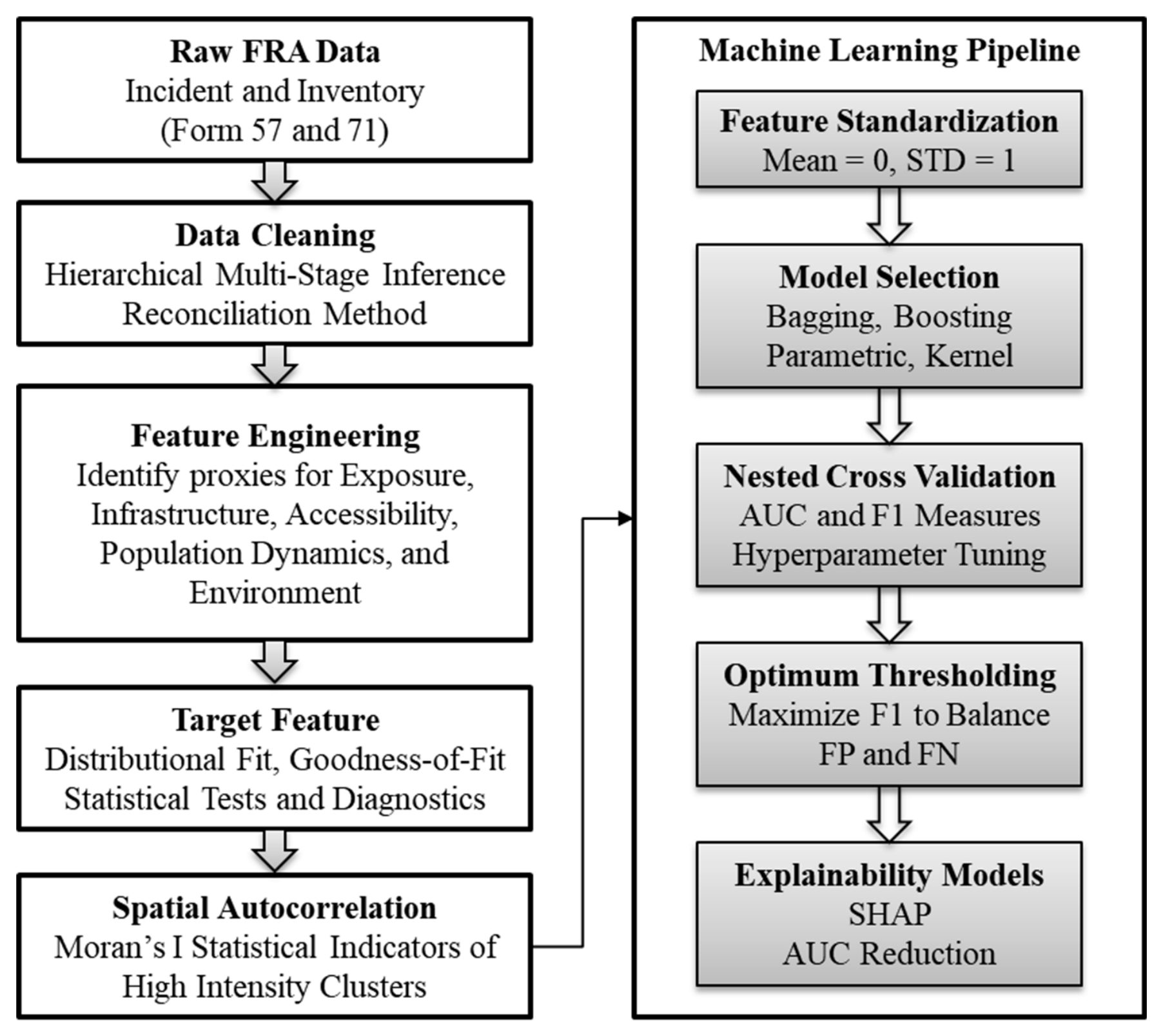
Figure 2.
Global distribution of the target feature, AIPC.
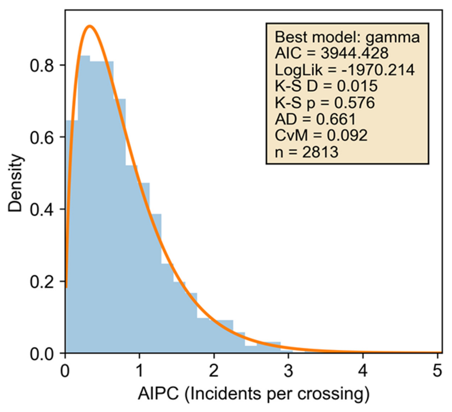
Figure 3.
Q-Q and P-P diagnostics for best fit Gamma.
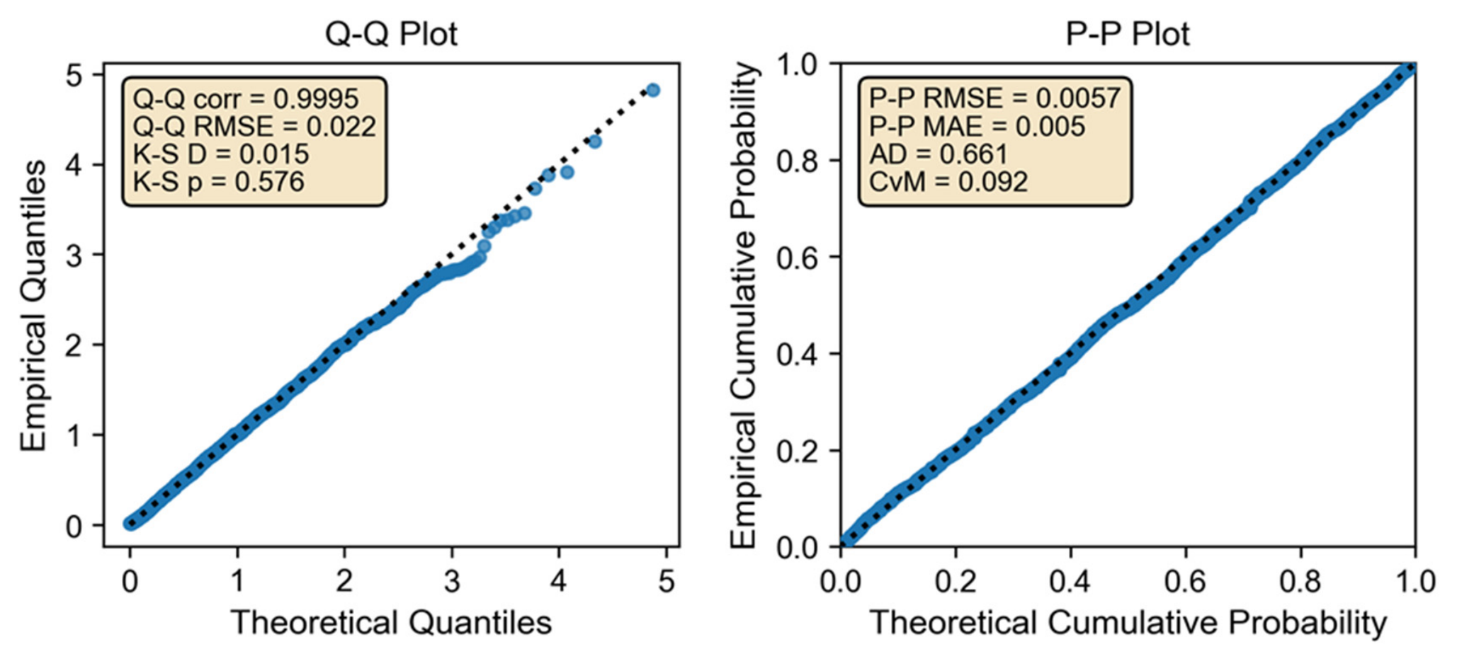
Figure 4.
Local Moran’s I classification of county-level (n = 3,108) AIPC (Queen contiguity weights, p < 0.05, 999 Monte Carlo permutations). HH = High–High; LL = Low–Low; HL = High–Low; LH = Low–High; NS = nonsignificant.
Figure 4.
Local Moran’s I classification of county-level (n = 3,108) AIPC (Queen contiguity weights, p < 0.05, 999 Monte Carlo permutations). HH = High–High; LL = Low–Low; HL = High–Low; LH = Low–High; NS = nonsignificant.
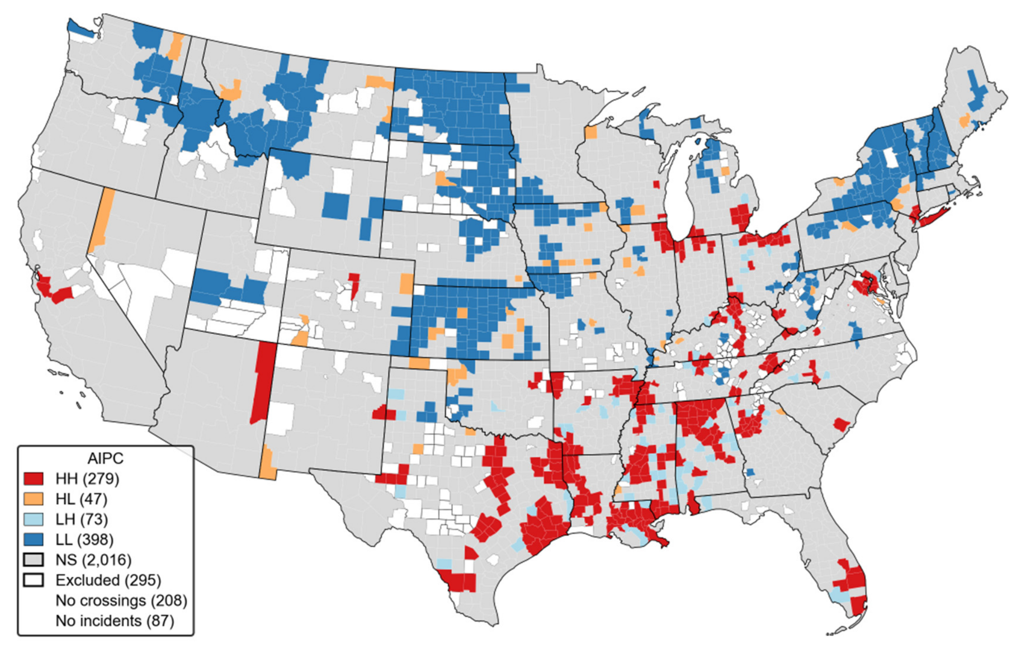
Figure 5.
Feature importance rankings for the extra trees (ET) model: (a) mean absolute SHAP values, and (b) mean AUC decrease under permutation, with error bars indicating ±1 standard deviation.
Figure 5.
Feature importance rankings for the extra trees (ET) model: (a) mean absolute SHAP values, and (b) mean AUC decrease under permutation, with error bars indicating ±1 standard deviation.
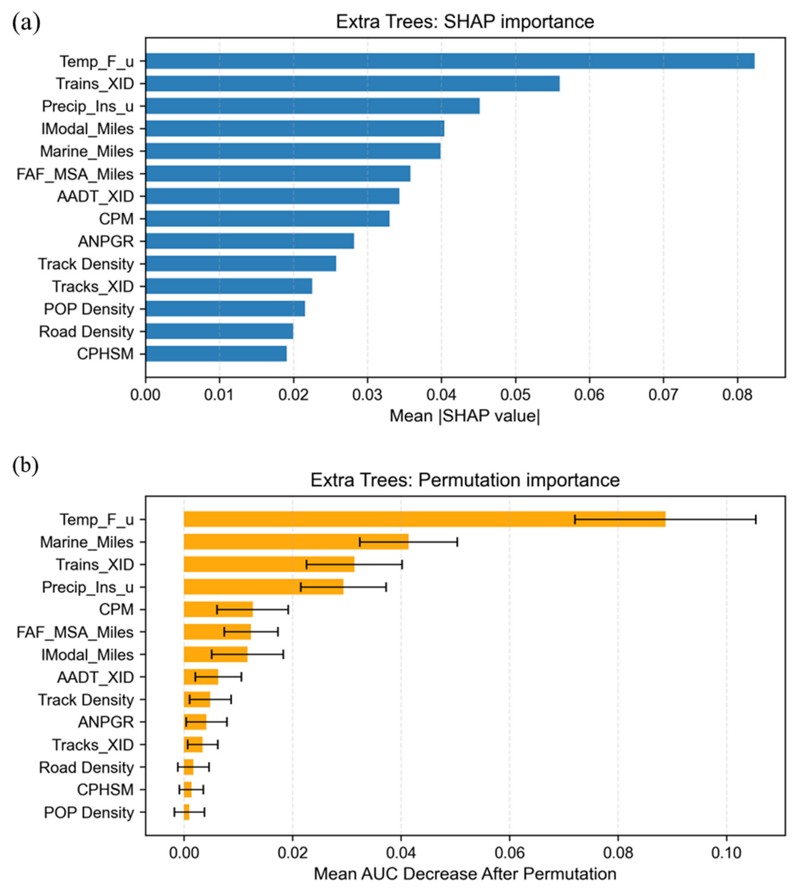

Table 1.
HRGC incident data cleaning results.
| Description | Filter | Retained | Removed |
|---|---|---|---|
| FRA Raw Incident Dataset | Already At-Grade Only | 250,290 | -- |
| Retain Public HRGC Only | Public/Private Code = “Y” | 226,170 | 21,120 |
| Retain CONUS Only | State FIP outside CONUS | 225,770 | 400 |
| Dropped County in Canada | State FIP = 099 | 225,768 | 2 |
| Reattributed Alaska/Hawaii | State FIP outside CONUS | 225,765 | 3 |
Table 2.
Selected features categories and their data sources.
| Feature Category |
ML Feature |
Description | Data Source |
|---|---|---|---|
| Incidents | Incidents (Public/Private Code = “Y”), 1975 to 2025 | [48] | |
| Crossings | Crossing Position = “At Grade”) and Crossing Type Code = 3 (Public) | [49] | |
| Trains_XID | Daily trains (non-missing) per crossing | ||
| Tracks_XID | Tracks per crossing. | ||
| CPM | Crossings per million population | ||
| AADT_XID | Average annual daily traffic (non-missing) per crossing. | ||
| CPHSM | Crossings per 100 square miles. | ||
| AIPC (Target) | Accumulated incidents per crossing for each county. | ||
| GIS | County shapefile containing land area in square-meters. | [50] | |
| GIS | Marine_Miles | Miles between county centroid and nearest marine highway. | [51] |
| GIS | FAF_MSA_Miles | Miles between county centroid and nearest metropolitan area centroid. | [52] |
| GIS | IModal_Miles | Miles between county centroid and nearest rail intermodal facility. | [53] |
| Population | ANPGR | County level average annual population growth rate from 2010 to 2020 | [54] |
| POP Density | County level population per square mile of land. | ||
| Infrastructure | Track Density | Track miles per 1,000 square miles of land. | [55] |
| Infrastructure | Road_Density | Road miles per square mile of land. | [56] |
| Climate | Temp_F_u | Average temperature (Fahrenheit) from 1901 to 2000. | [57] |
| Climate | Precip_Ins_u | Average precipitation (inches) from 1901 to 2000. | [58] |
Table 3.
Statistical tests comparing model fit.
| Model | AIC | LogLik | KS | KS_p | AD | CvM | k | α | μ | σ |
|---|---|---|---|---|---|---|---|---|---|---|
| Gamma | 3944.4 | -1970.2 | 0.015 | 5.8E-01 | 0.661 | 0.092 | 2 | 1.71 | 0.00 | 0.47 |
| Weibull | 3954.2 | -1975.1 | 0.016 | 4.3E-01 | 0.853 | 0.117 | 2 | 1.38 | 0.00 | 0.88 |
| GMM_2_log | 3961.2 | -1975.6 | 0.019 | 2.7E-01 | 0.916 | 0.140 | 5 | 0.7, 0.3 | -0.2, -1.3 | 0.6, 0.9 |
| Skew-Normal | 3987.7 | -1990.8 | 0.034 | 2.5E-03 | 4.639 | 0.849 | 3 | 52.06 | 0.04 | 0.97 |
| Johnson SU | 4045.5 | -2018.8 | 0.029 | 1.7E-02 | 4.077 | 0.579 | 4 | -7.30 | -0.17 | 0.02 |
| Log-Normal | 4259.1 | -2127.6 | 0.067 | 1.7E-11 | 25.319 | 4.045 | 2 | 0.89 | 0.00 | 0.58 |
| Exponential | 4361.8 | -2179.9 | 0.117 | 6.8E-34 | 78.521 | 13.510 | 1 | 1.0 | 0.00 | 0.80 |
Table 4.
Cross-validated performance of candidate models. RRT = relative runtime, normalized to logistic regression (LR = 1.0). Underlined hyperparameter values in a set indicate the selection for each model.
Table 4.
Cross-validated performance of candidate models. RRT = relative runtime, normalized to logistic regression (LR = 1.0). Underlined hyperparameter values in a set indicate the selection for each model.
| Model | AUCμ | AUCσ | F1μ | F1σ | RRT | Hyperparameters and Search Region | τ*μ | τ*σ |
|---|---|---|---|---|---|---|---|---|
| ET | 0.907 | 0.016 | 0.528 | 0.064 | 22.7 |
NT = {100, 200, 300}, Dmax = {5, 8, 12, none}, Smin = {2, 4, 8}, Lmin = {1, 2, 5} |
0.360 | 0.072 |
| XGB | 0.905 | 0.012 | 0.534 | 0.039 | 6.8 |
NT = {100, 200, 300}, NL = {3, 5, 8}, Dmax = {5, 8, 12, none}, RL = {0.1, 1.0, 3.0}, Lmin = {1, 2, 5}, NS = {0.8}, CS = {0.8}, λR = {1.0, 3.0} |
0.533 | 0.129 |
| RF | 0.900 | 0.015 | 0.525 | 0.039 | 27.3 |
NT = {100, 200, 300}, Dmax = {5, 8, 12, none}, Smin = {2, 4, 8}, Lmin = {1, 2, 5} |
0.297 | 0.072 |
| LGB | 0.899 | 0.014 | 0.516 | 0.021 | 5.1 |
NT = {100, 200, 300}, NL = {3, 5, 8}, RL = {0.1, 1.0, 3.0}, Dmax = {8, 12, none}, NS = {0.8}, CS = {0.8} |
0.455 | 0.108 |
| CB | 0.896 | 0.017 | 0.524 | 0.053 | 4.9 |
NT = {100, 200, 300}, RL = {0.1, 1.0, 3.0}, Dmax = {4, 6, 12} |
0.263 | 0.033 |
| SVM | 0.872 | 0.016 | 0.457 | 0.054 | 12.7 |
C = {0.5, 1.0, 2.0}, Kernel = {linear, RBF}, γ = {scale, auto} |
0.225 | 0.027 |
| LR | 0.859 | 0.025 | 0.444 | 0.040 | 1.0 |
C = {0.1, 1.0, 10.0}, Solver = {lbfgs, liblinear} |
0.685 | 0.015 |
Disclaimer/Publisher’s Note: The statements, opinions and data contained in all publications are solely those of the individual author(s) and contributor(s) and not of MDPI and/or the editor(s). MDPI and/or the editor(s) disclaim responsibility for any injury to people or property resulting from any ideas, methods, instructions or products referred to in the content. |
© 2026 by the author. Licensee MDPI, Basel, Switzerland. This article is an open access article distributed under the terms and conditions of the Creative Commons Attribution (CC BY) license.
Copyright: This open access article is published under a Creative Commons CC BY 4.0 license, which permit the free download, distribution, and reuse, provided that the author and preprint are cited in any reuse.


