

Submitted:
27 May 2026
Posted:
28 May 2026
You are already at the latest version
Abstract
We consider quasi-one-dimensional (Q1D) continuous waves (CWs) in the two-dimensional (2D) optical system with the cubic-quintic nonlinearity and a Q1D potential trough. In the case of a smooth trough profile, we confirm the known modulational instability (MI) of Q1D CWs with the transverse structure corresponding to the 1D ground state (GS) in the potential trough, and demonstrate the MI of CWs with the dipole-mode (DM) transverse structure, corresponding to the lowest 1D excited state in the potential trough. The CWs of both GS and DM types remain nearly stable close to edges of their existence regions. Stable stationary states in the form of periodic chains of 2D solitons, trapped in the potential trough, are produced in a numerical form. The dynamics of the soliton chains excited by a localized kick is studied too. For the potential trough with the singular delta-functional profile, we find two species of exact analytical solutions for CWs, one of which is completely stable.
Keywords:
cubic-quintic nonlinearity
; modulational instability
; Bogoliubov - de Gennes equations
; soliton chains
; delta-functional potential
; exact solutions
1. Introduction and the Models
Spatial-domain propagation of light in bulk waveguides is determined by the interplay of diffraction and material nonlinearity. This setting gives rise to a variety of self-supporting modes, including solitons [1,2,3], vortices [4,5,6,7] (similar to their counterparts in atomic Bose-Einstein condensates (BEC) [8,9]), skyrmions [10,11], etc., which are adequately modeled by the two-dimensional (2D) nonlinear Schrödinger (NLS) equation, or a coupled system of such equations [12,13]. Spatiotemporal light propagation in planar waveguides is accurately modeled by 2D NLS equations which are essentially identical to their counterparts in the spatial domain [14]. While the ubiquitous nonlinearity of optical materials is represented by the Kerr cubic term, accurate experiments were also performed in chalcogenide glasses [15] and colloidal suspensions of metallic particles [16], which are adequately represented by combined nonlinearities – most typically, cubic-quintic (CQ) ones, which feature the competition of the cubic self-focusing and quintic defocusing.
While 1D solitons are typically stable states, the stability is a major challenge for studies of 2D nonlinear modes in optics, as well as in other areas of physics, especially in BEC [14,17]. The basic problem is the critical collapse which destabilizes 2D fundamental solitons under the action of the cubic self-focusing [12,13], while the solitons with embedded vorticity are still more vulnerable to the splitting instability [18]. Two major mechanisms which provide stabilization of both the fundamental (zero-vorticity) and vortex optical solitons in 2D rely upon the use of the CQ nonlinearity and/or effective potentials, which represent the transverse modulation of the refractive index in the waveguide. In particular, the CQ nonlinearity readily stabilizes a part of the vortex-soliton states, with different values of the topological charge (vorticity), against the splitting [19,20]. On the other hand, spatially periodic (lattice) potentials, both fully two-dimensional (2D) [21,22] and quasi-one-dimensional (Q1D) ones, which depend on a single coordinate [23,24]), also secure the stabilization of the fundamental and vortex solitons (although the lattice potentials destroy the underlying spatial isotropy, vortex solitons with a nonzero topological charge can be defined in this case too [21,22]).
The most basic 2D model combining the CQ nonlinearity and spatial inhomogeneity includes a Q1D potential trough, which depends on the single transverse coordinate, x, and does not depend on the other coordinate, y [25]. The corresponding scaled NLS equation for the slowly varying amplitude of the optical wave, , is
where z is the propagation distance, is the strength of the quintic self-defocusing nonlinearity (while the strength of the cubic self-focusing is set to be 1 by scaling), and is the depth of the potential trough with the Gaussian profile, whose width is also fixed to be 1 by means of scaling.
Equation (1) applies as well to the spatiotemporal light propagation in a planar waveguide with anomalous group-velocity dispersion, In that case, x remains the transverse coordinate, while is the temporal variable, with t and being the scaled time and group velocity of the carrier wave. In the spatiotemporal setting, the trough potential represents a stripe of a material with an enhanced refractive index, embedded into the planar waveguide. In the latter case, solely the Q1D effective potential is possible, because it cannot be made a function on time.
Fully localized states, predicted as solutions of Eq. (1), are characterized by the value of the 2D integral power in the spatial domain (or energy in the spatiotemporal one),
which is a dynamical invariant of Eq. (1). Other conserved quantities are the Hamiltonian,
and the y-component of the momentum, , where * stands for the complex conjugate.
The simplest stationary states admitted by Eq. (1) are continuous waves (CWs), which are solutions trapped in the potential trough and thus localized in the x direction, while their y dependence is represented by a real wavenumber q:
Here, k is a real propagation constant, and a real modal function obeys the the transverse equation:
Using the obvious Galilean invariance of Eq. (1) in the y direction, it is sufficient to consider the CW solutions with , which is done below, the respective CW solution being independent of y. Then, Eq. (4) produces bound states (solutions localized at ) for .
Equation (4) is the 1D stationary NLS equation with the Gaussian trapping potential, Therefore, it is natural to classify its bound-state solutions as a nonlinear extension of eigenstates which are produced by the linear Schrödinger equation with the trapping potential, in the small-amplitude limit. Accordingly, the bound states are classified as the spatially even () ground state (GS), spatially odd () first excited state (alias the dipole mode, DM), spatially even second excited state (alias the quadrupole mode), etc.
The basic problem for CW solutions is their modulational instability (MI, alias the Benjamin-Feir instability [26]) against small perturbations which impose periodic modulation of the CW state along the free coordinate y [27,28,29,30,31,32,33]. In particular, MI plays the crucial role in the generation of rogue waves [34,35,36,37,38]. For the CW solutions of Eq. (1) with the GS transverse structure, this problem was originally addressed in Ref. [25]. In the presents work, we aim to further elaborate this topic. First, in Section 2 we recapitulate the MI analysis performed in the framework of Eq. (1), including new findings for the CWs with the DM transverse structure. While all the CWs are subject to MI, the instability is very weak for the CWs of both the GS and DM types, with values of the propagation constant close to existence boundaries of these solution families, the respective interval of the “practical stability" being wider for the DMs than for GSs.
It is natural to expect that MI may split the CW into a periodic chain of 2D solitons along the y coordinate, trapped in the potential trough. In Section 3, we produce a numerical solution for the stationary soliton chain and demonstrate its stability. We also report results produced by the application of a kick to a particular soliton in the chain. The kick, that may be directed along x or y, eventually generates a complex dynamical picture.
The most essential novel results are reported in Section 4 for the 2D model with the CQ nonlinearity and the potential trough, , represented by the delta-functional profile:
Factor is introduced in Eq. (5) to keep the same transverse area of the trough potential, , as in Eq. (1). We obtain two families of exact analytical solutions of Eq. (5), in parameter regions
where the critical potential strength is
The numerical analysis demonstrates that, while the exact solutions are subject to MI in Case 1, they are completely stable in Case 2. The possibility to produce stable CW states in the form of Q1D bright solitons, supported by the trough potential, is a remarkable finding (in particular, because the stable solutions are obtained here in the analytical form), which was not reported for previously studied models. In this connection, it is relevant to mention that it was demonstrated in Ref. [39] that a Q1D (stripe-shaped) dark soliton may be stabilized against MI, in the framework of the two-dimensional NLS equation with the cubic self-defocusing term (the quintic one is not needed in this case), by means of a sufficiently strong Q1D potential ridge (rather than the trough), which corresponds to in Eq. (1).
The paper is concluded by Section 5, which summarizes the obtained results and puts forward possibilities for additional studies on the present topic.
2. MI (Modulational Instability) of the Q1D (Quasi-One-Dimensional) CW States
2.1. Linearized Equations for Modulational Perturbations
To analyze the modulational (in)stability of the CW states, a perturbed solution is looked for as
where is a real solution of Eq. (4) with propagation constant k (recall we set in Eqs. (3) and (4)), and are components of the eigenmode of small perturbations, with a real infinitesimal amplitude and wavenumber p, and is the corresponding eigenvalue, the stability condition being for all real p. The substitution of ansatz (8) in Eq. (1) and linearization with respect to leads to the system of linear equations for the perturbation eigenmode (the Bogoliubov-de Gennes (BdG) equations, in terms of the BEC theory [40]):
The analysis of the CW states and their stability may be performed treating and as control parameters, while is a free parameter of the family of the CW states.
2.2. The MI of the CW States with the Ground-State (GS) Transverse Structure
In the uniform space, with in Eq. (1), the transverse profile of the CW state is given by the well-known Q1D soliton solution of Eq. (1) [41]:
in which the propagation constant k takes values in the interval
The total 1D power of soliton (11),
diverges in the limit of , when the soliton expands into a CW state in the x direction.
Typical examples of the stationary GSs, produced by the numerical solution of Eq. (4) with and , are plotted in Figure 1. The solutions were produced by means of the modified squared-operator method (MSOM) [42] in the spatial domain of size , discretized on a mesh of 128 points, with the mesh size . They may be construed as solitons trapped in the potential well. For fixed values of parameters and g, the CW family is characterized by the dependence of the 1D power P on k, cf. Eq. (13) for . In particular, a set of curves for and different values of is plotted in Figure 2. At , each curve starts from the eigenvalue which, in terms of quantum mechanics, is determined by the GS energy, , of the potential well . With the increase of of P, the curves with attain their turning points, , and then move back, in the direction of , as shown by the dashed lines in Figure 2. The extension of the curves towards will bring them asymptotically close to the value , see Eq. (12).
In agreement with Ref. [25], the numerical solution of the BdG system of Eqs. (9) and () demonstrates that all CW modes of the GS type are indeed subject to the MI, as the solution always produces eigenvalues with . As an example, dependences of on p for and are plotted in Figure 3, for different values of the 1D power P.
The CW instability, predicted by the MI analysis, was confirmed by direct simulations of the perturbed evolution of the CW states, which were carried out in the framework of Eq. (1), by means of the usual split-step Fourier-transform method (here and below, the simulations were performed with stepsize ). In particular, results of the simulations for the CW state with the central GS profile from Figure 1, which is characterized by he largest MI gain, , for the parameters fixed in Figure 1, viz., and , are displayed in Figure 4. It demonstrates that, in the plane, the instability splits the original Q1D CW state into a chain of localized 2D speckles, which performs irregular oscillations.
The CW states corresponding to other values of eigenvalue k in Eq. (4), which are taken closer to the linear limit, i.e., lower edge of the respective curve (see Figure 2), demonstrate much weaker MI, so that, in direct simulations, they may seem as practically stable states. An example is presented in Figure 5, for , , and , , It is obvious that this CW state, for which the numerical solution of the BdG equations (9) and () yields a very small peak value of the MI gain, , indeed exhibits virtually no instability. On the other hand, CWs with large values of P, such as and in Figure 3, may also demonstrate practical stability, explained by the domination of the self-defocusing quintic nonlinearity in this case.
2.3. The MI of the Dipole-Mode (DM) CWs
CW states of the DM type were not studied in previous works in the framework of Eqs. (1) and (4), or in similar models (cf. Ref. [25]). Note that, unlike the 1D soliton (11), Eq. (1) in the free space (with ) does not have solutions of the DM type.
Families of numerically found stationary CWs of the DM type are represented by the respective curves in Figure 6(a) for and different values of g, where is the same 1D power as defined above. Like their GS counterparts (cf. Figure 2), the curves originate, at , from eigenvalues k corresponding to the first excited state in the quantum-mechanical potential , reach turning points at , and with further increase of P move back in the direction of , as shown by dashed lines in Figure 6(a). Figure 5(b) demonstrates the DM profiles for two widely different values of the 1D power, and , which corresponds to markers a and b in panel (a), for . Lastly, Figure 5(c) exhibits spectra of the MI gain for these CW states.
In agreement with the predictions of the MI analysis, direct simulations of the perturbed evolution of the CW states of the DM type demonstrate strong instability when the respective MI gain, , is relatively large, and “practical stability" when the MI gain is small, see typical examples displayed in Figure 7 and Figure 8, respectively. The strong MI splits the flat CW into a randomly oscillating chain of localized speckles, which keep the original dipole structure. It is relevant to stress that the region of the “practical stability" for the CW states of the DM type is essentially broader than for their GS counterparts. Similar to what is concluded above for the CW states of the GS type, the effective stabilization for the DM CWs may be provided, as in Figure 8, by a sufficiently large value of strength g of the defocusing term ( in Figure 8), or by a large value of the 1D power, which also makes the defocusing nonlinear term a dominant one. For instance, in the same case of and as in Figure 7, but with the power larger by a factor , the CW of the DM types seems to be fully stable in direct simulations (not shown here in detail)..
We have also investigated CW states which correspond, in the linear limit, to the second-order (quadrupole) bound state in the trapping potential . They always demonstrate strong MI, without any interval of the “practical stability", therefore they are not considered in detail here.
3. Stationary Chains of 2D Solitons
3.1. The Existence and Stability of the Chains
While, as shown in Figure 4, the MI splits the unstable CW states with the GS transverse structure into a chain of localized speckles in the state of random oscillations, it is natural to expect that the same Eq. (1) may produce a stationary chain of 2D solitons, arranged periodically along the y axis. Such a chain may be considered as a manifestation of the MI in terms of stationary states.
Here, we report numerical results for the chains, systematically collected for parameters and in Eq. (1), which makes it possible to exhibit generic findings. The stationary-chain solutions with propagation constant k were looked for as
with real function satisfying the equation (written with the above-mentioned values , )
cf. Eq. (4). The chain solutions were obtained by means of MSOM applied to Eq. (15), starting with the y-periodic input,
The numerical solutions were constructed in the computational domain with grid points, periodic boundary conditions in the direction, and zero boundary conditions at . The same boundary conditions were adopted in dynamical simulations of Eq. (1).
The soliton-chain family, produced by the numerical solution of Eq. (15), is presented in Figure 9 by means of the dependence of the 2D integral power (2) on the propagation constant k. The curve features a turning point at , which connects two branches with opposite slopes. The bottom branch originates, at , from , which corresponds to the eigenstate of the respective 2D linear Schrödinger equation. Stability of the soliton chains belonging to the continuous blue part of the curve in Figure 9 was established by the computation of the respective eigenvalues , as per the BdG system of Eqs. (9) and (), and verified by direct simulations of the perturbed propagation.
Two representative chain solutions, belonging to the bottom and top branches of the curve, which are marked (a) and (b) in Figure 9, are displayed in Figure 10, by means of the respective distributions of , with amplitudes and (in agreement with the fact that the power at point (b) in Figure 9 is essentially higher than at point (a)). Adjacent peaks in both chains keep alternating signs, inherited from the input given by Eq. (16).
3.2. Response of the Soliton Chains to Localized Kicks
To further examine the robustness of the solitons chains and their intrinsic dynamics, we applied a localized phase kick to the single soliton, whose center is located at in the stable chain marked (b) in Figure 9 (the stationary shape of the chain is plotted in Figure 10(b)). The evolution excited by the kick was observed in direct simulations of Eq. (1).
First, the kick is applied in the y direction, which is represented by the initial condition
where is the stationary soliton-chain solution,
is the 2D Gaussian mask, with widths and matched to the transverse dimensions of the individual soliton in the chain, and real Q is the strength of the kick. Here, we display the results for , which represents a generic case.
The results of the simulations, up to , are displayed in Figure 11. The chain structure remains essentially undisturbed at , which is followed by the emission of a disturbance wave from the kicked soliton in the directions. Due to the periodic boundary conditions, the disturbances re-enter from the opposite edges of the computational domain, making the cumulative effect visible at . As a result, an irregular pattern appears at . This effect depends on the size (period) of the domain in the y direction, as confirmed by simulations performed in the domain with the double size, : the onset of the complex pattern is delayed, and the disturbance waves re-enter from the opposite edge at (not shown here in detail).
4. CWs Maintained by the Delta-Functional Trapping Potential
4.1. Analytical Results
The substitution of the usual ansatz for the stationary CW state, , in Eq. (5) leads to the real equation for , cf. Eq. (4):
The GS solution to Eq. (20) for an even function must be continuous at , with the jump of the first derivative, imposed by the delta-functional potential:
A commonly known fact is that the linearized version of Eq. (20) supports precisely one bound state, in the form of
It is possible to construct two exact solutions for the soliton pinned to the delta-functional potential. First, in Case 1, defined as per Eqs. (6) and (7), i.e., for , the exact solution can be constructed in the following interval of values of the propagation constant,
where the left edge naturally coincides with the eigenvalue (22) of the linearized equation (20). If condition (23) holds, one easily finds a solution, combining the usual exact soliton (11) in the free space (with ) and the jump condition (21):
with the spatial shift determined as a root of equation
An explicit solution of Eq. (25) is given by a cumbersome expression:
In the opposite Case 2, also defined as per Eqs. (6) and (7), i.e., as , another exact solution for the soliton pinned to the delta-functional potential can be found in the following interval of values of the propagation constant:
cf. interval (23). In this case, the right edge of the existence interval coincides with the eigenvalue (22) of the linearized equation (20). The solution existing in interval (27) is based on the following singular exact solution of Eq. (20) in the free space (with ),
In the free space, the singular solution is irrelevant. However, in the presence of the delta-functional potential, an exact solution for the pinned soliton can be obtained from expression (28), replacing x by :
4.2. Numerical Results
The accuracy and stability of the above analytical solutions were verified by comparison with numerical solutions obtained from Eqs. (5) and (20) with the delta-function approximated by a narrow Gaussian,
with a small regularization scale , where . is the above-mentioned mesh size adopted in realization of the MSOM algorithm. This value is definitely much smaller than characteristic length scales, in the x direction, of all solutions considered here. However, this approximation cannot exactly reproduce the cusp at the center of exact analytical solutions (24) and (29) for the pinned solitons, see Figure 14 below.
Figure 13.
An example of the MI destroying the CW based on the stationary profile (24) (corresponding to Case 1, see Eq. (6)). The parameters are , , . (a) The initial intensity profile . (b) The MI gain, , versus p, showing the instability band with the peak value , attained at . (c) The evolution of the local intensity in cross-section , initiated by the perturbed input (33) with and . The CW breakup commences at .
Figure 13.
An example of the MI destroying the CW based on the stationary profile (24) (corresponding to Case 1, see Eq. (6)). The parameters are , , . (a) The initial intensity profile . (b) The MI gain, , versus p, showing the instability band with the peak value , attained at . (c) The evolution of the local intensity in cross-section , initiated by the perturbed input (33) with and . The CW breakup commences at .
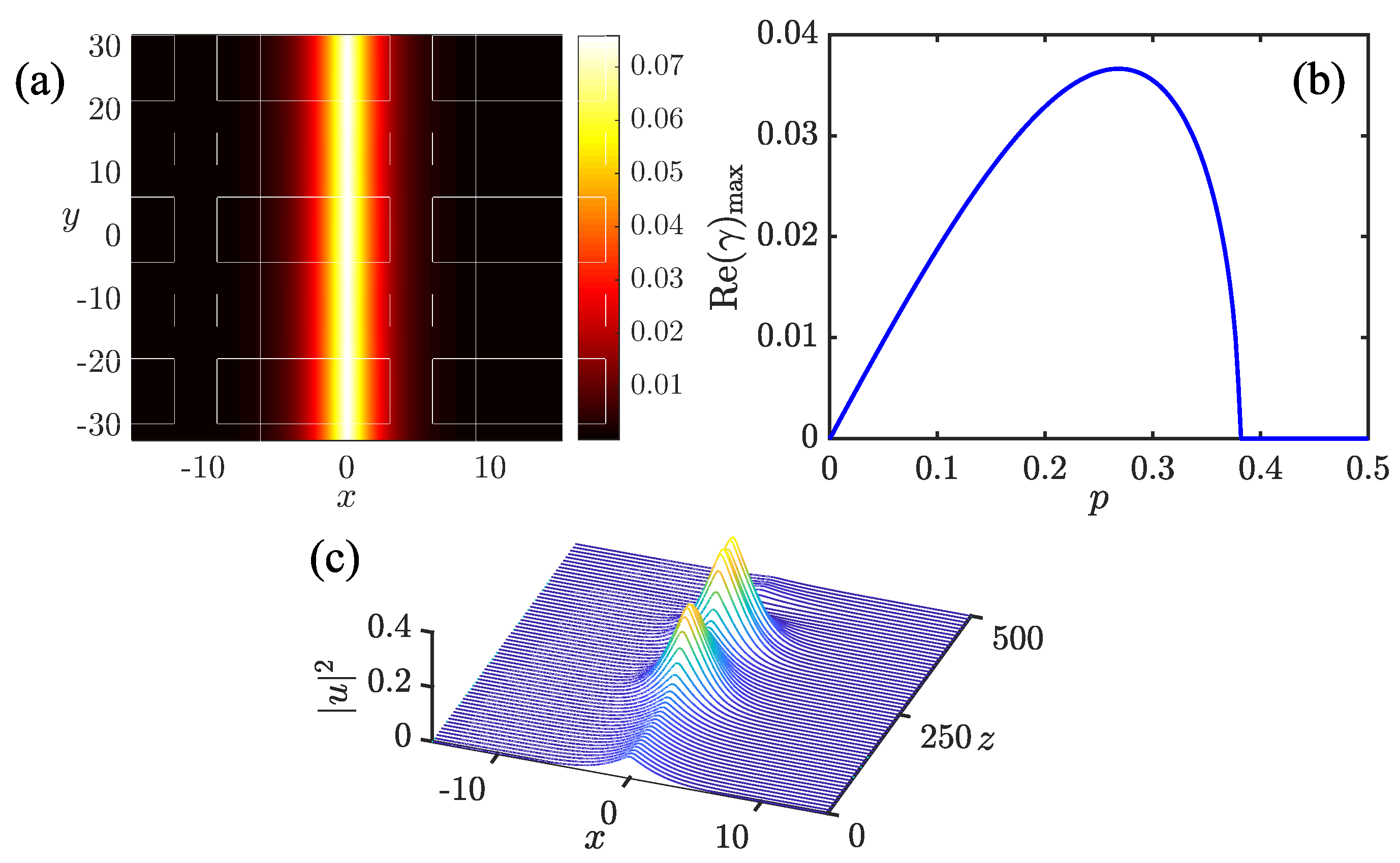
Figure 14.
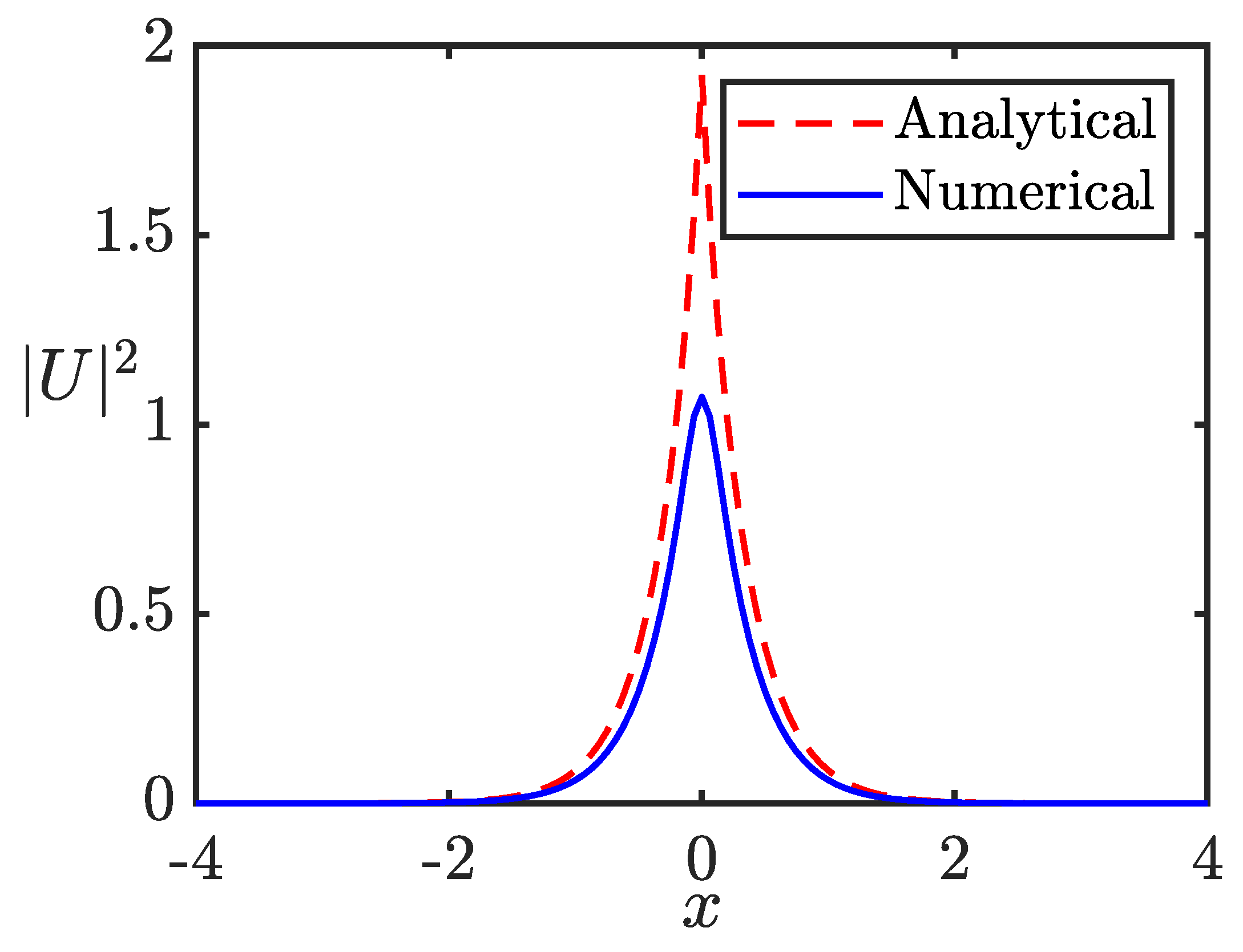
An example of the transverse profile of a modulationally stable CW. The analytical profile is produced by Eqs. (29) and (31), with and . Its numerically found counterpart cannot exactly reproduce the cusp of the analytical solution, determined by the jump condition (21).
First, both the numerical computation of the stability eigenvalues, as per the BdG system of Eqs. (9) and (), and direct simulations of the perturbed evolution easily demonstrate that, in terms of the 1D reduction of Eq. (5) (excluding coordinate y), all pinned states of both types, (24) and (29), are completely stable. However, in the framework of the full 2D equation (5), all the CW states based on the 1D solitons of type (24) are subject to MI, see a typical example in Figure 13. In particular, the direct test of the perturbed propagation, displayed in Figure 13(c), was performed by simulating Eq. (20) with the initial condition
where is the stationary profile, p and being the wavenumber and amplitude of the modulational perturbation (cf. Eq. (8)).
In view of the full instability of the CWs with the stationary profile (24), we do not consider this case in further detail, and focus on the CWs with the transverse profile (29), which turn out to be completely stable. First, an example of this profile for , and is plotted in Figure 14.
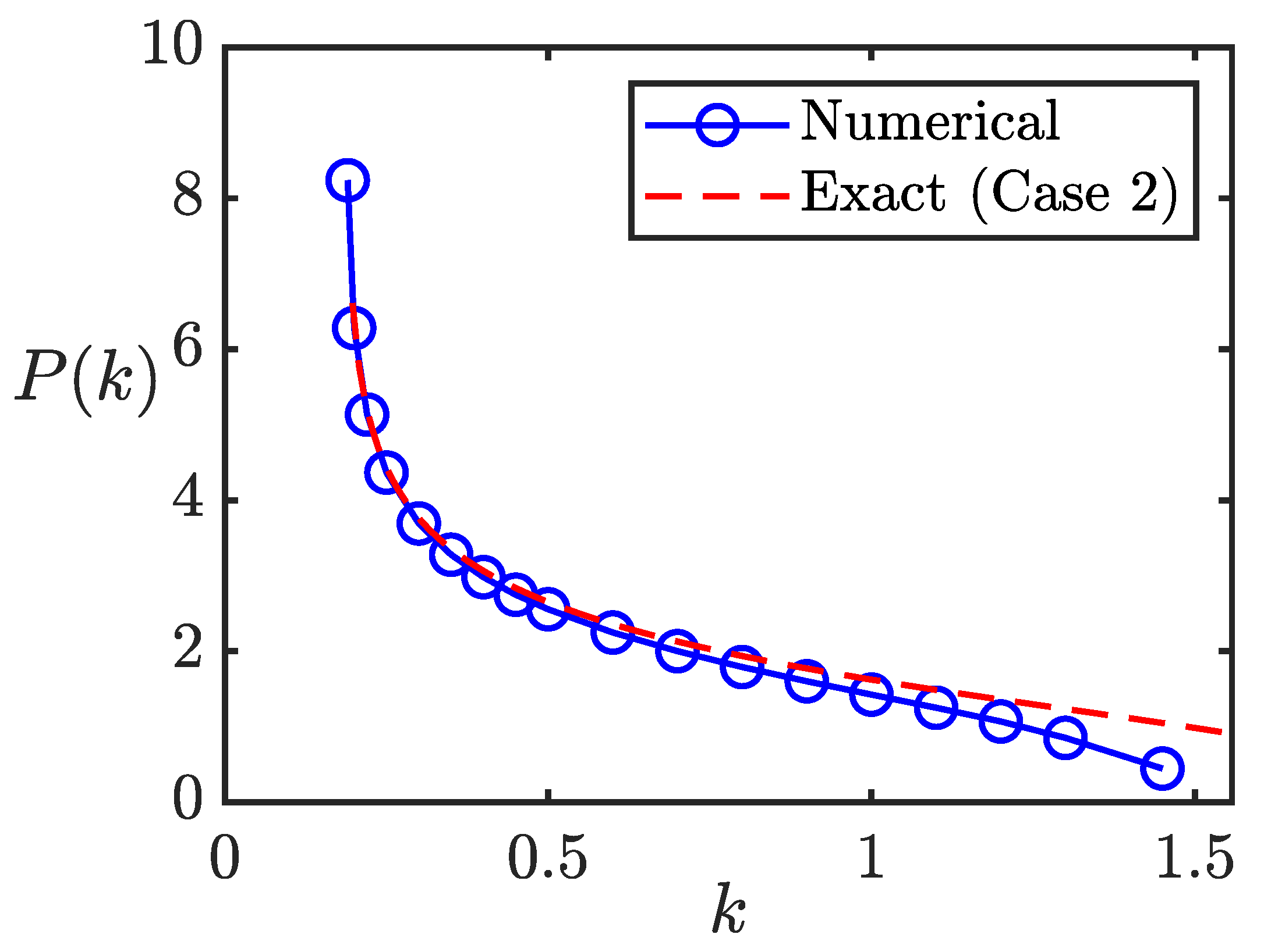
Further, a family of such profiles, with the same parameters , and varying values of k, is displayed in Figure 15, by means of the respective dependence of the 1D power P on the propagation constant k. In fact, the power of the analytical solution diverges in the limit of , which represents the left edge of the existence region in Figure 15.
Note that the curve in Figure 15 obeys the anti-Vakhitov-Kolokolov(anti-VK) criterion, , which is known as the necessary stability condition for self-trapped states dominated by self-repulsive nonlinearity [43], which is the case here, because the pinned solitons of type (29) do not exist in the absence of the self-defocusing quintic term in Eq. (5) (the VK criterion proper, , is the necessary stability condition for solitons supported by self-attractive nonlinearity [44,45])
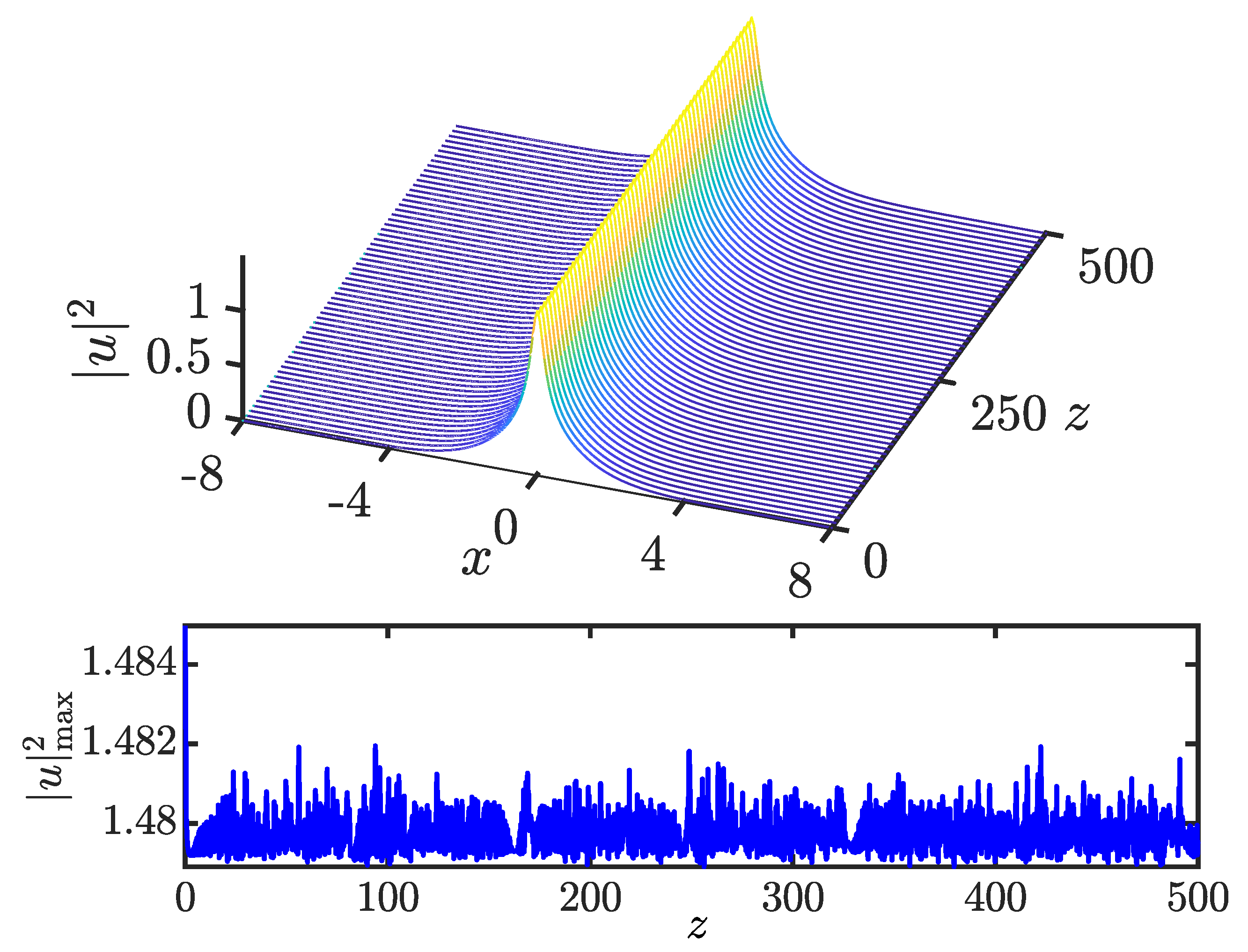
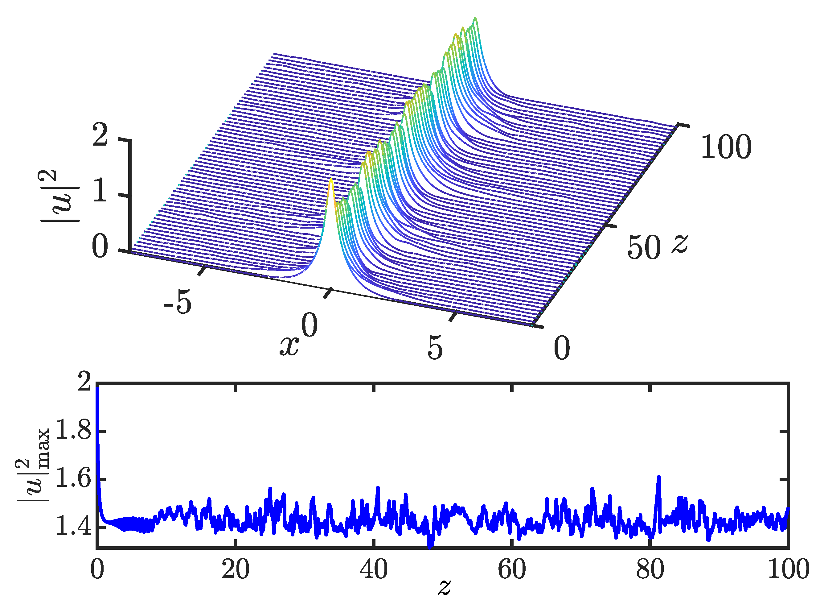
An illustration of the stability of the CW with the transverse profile provided by Eqs. (29) and (31), with , , , is provided by Figure 16, in which the simulated propagation of the CW state, including initial perturbation (33) with and , is displayed. To additionally test the CW robustness, a similar simulation is displayed in Figure 17 for the perturbation with a much larger amplitude, . It is clearly observed that the CW is not destroyed even by strong perturbations.
5. Conclusion
The objective of this work is to consider the dynamics of Q1D (quasi-one-dimensional) CW (continuous-wave) states and related patterns (such as chains of 2D solitons) in the optical medium with the CQ (cubic-quintic) nonlinearity and the trapping potential trough. In the model with the usual smooth trapping trough, we have briefly reproduced the known MI (modulational instability) of CW states with the transverse structure corresponding to the GS (ground state) of the trapping potential, and produced new results for the CW states with the transverse DM (dipole-mode) structure, which corresponds to the first excited state of the potential trap. In particular, it is found that the CWs of both types, GS and DM, are “practically stable" near edges of their existence domains. Then, stable periodic chains of 2D solitons with alternating signs, maintained by the potential trough, have been found as the stationary manifestation of the MI, and their dynamics, initiated by the application of localized kicks, was explored. An essentially novel finding is represented by two families of exact CW solutions in the model with the delta-functional trapping potential, a remarkable result being the complete stability of one family, which does not exist without the trapping potential.
As an extension of the analysis, it may be interesting to consider chains of 2D solitons with embedded vorticities, identical or alternating (in the latter case, these are vortex-antivortex chains), trapped in the Q1D potential. It is known that individual vortex solitons with unitary and multiple topological charges have their stability regions in the free-space NLS equation with the CQ nonlinearity [19,20], therefore the trapped chain may be stable too. As a dynamical problem, one may address collisions between counterpropagating 2D solitons moving in the potential trough.
Author Contributions
Methodology, Boris A. Malomed; Software, Thawatchai Mayteevarunyoo; Validation, Thawatchai Mayteevarunyoo and Boris A. Malomed; Investigation, Boris A. Malomed; Data curation, Thawatchai Mayteevarunyoo and Boris A. Malomed; Writing – original draft, Boris A. Malomed; Writing – review & editing, Thawatchai Mayteevarunyoo and Boris A. Malomed; Supervision, Boris A. Malomed. All authors have read and agreed to the published version of the manuscript.
Funding
This research received no external funding.
Data Availability Statement
The original contributions presented in this study are included in the article. Further inquiries can be directed to the corresponding author.
Conflicts of Interest
The authors declare no conflicts of interest.
References
- Kivshar, Y. S.; Luther-Davies, B. Dark optical solitons: physics and applications. Phys. Rep. 1998, 298, 81–197. [Google Scholar] [CrossRef]
- Kivshar, Y. S.; Agrawal, G. P. Optical Solitons: From Fibers to Photonic Crystals; Academic Press: San Diego, 2003. [Google Scholar]
- Dauxois, T.; Peyrard, M. Physics of Solitons; Cambridge University Press: Cambridge, 2006. [Google Scholar]
- Shen, Y.; Wang, X.; Xie, Z.; Min, C.; Fu, X.; Liu, Q.; Gong, M.; Yuan, X. Optical vortices 30 years on: OAM manipulation from topological charge to multiple singularities. Light Sci. Appl. 2019, 8, 90. [Google Scholar] [CrossRef] [PubMed]
- Quinteiro Rosen, G. F.; Tamborenea, P. I.; Kunn, T. Interplay between optical vortices and condensed matter. Rev. Mod. Phys. 2022, 94, 035003. [Google Scholar] [CrossRef]
- Zhang, H.; Zeng, J.; Lu, X.; Wang, Z.; Zhao, C.; Cai, Y. Review on fractional vortex beam. Nanophotonics 2022, 11, 241–273. [Google Scholar] [CrossRef] [PubMed]
- Chen, S.; Chen, J.; Xia, T.; Xie, Z.; Huang, Z.; Zhou, H.; Liu, J.; Chen, Y.; Li, Y.; Yu, S.; Fan, D.; Yuan, X. Optical vortices in communication systems: mode (de)modulation, processing, and transmission. Adv. Photonics 2025, 7, 044001. [Google Scholar] [CrossRef]
- Fetter, A. L. Rotating trapped Bose{Einstein condensates. Rev. Mod. Phys. 2009, 81, 657–691. [Google Scholar] [CrossRef]
- Sakaguchi, H. New models for multi-dimensional stable vortex solitons. Front. Phys. 2018, 14, 12301. [Google Scholar] [CrossRef]
- Karnieli, A.; Tsesses, S.; Bartal, G.; Arie, A. Emulating spin transport with nonlinear optics, from high-order skyrmions to the topological Hall effect. Nat. Commun. 2021, 12, 1092. [Google Scholar] [CrossRef]
- Shen, Y. J.; Zhang, Q.; Shi, P.; Du, L. P.; Yuan, X. C.; Zayats, A. V. Optical skyrmions and other topological quasiparticles of light. Nat. Photonics 2024, 18, 15–25. [Google Scholar] [CrossRef]
- Sulem, C.; Sulem, P.-L. The Nonlinear Schrödinger Equation: Self-Focusing and Wave Collapse; Springer: New York, 1999. [Google Scholar]
- Fibich, G. The Nonlinear Schrödinger Equation: Singular Solutions and Optical Collapse; Springer: Heidelberg, 2015. [Google Scholar]
- Malomed, B. A.; Mihalache, D.; Wise, F.; Torner, L. Spatiotemporal optical solitons. In Optics B: Quant. Semicl. Opt. J.; 2005; Volume 7, pp. R53–R72. [Google Scholar]
- Boudebs, G.; Cherukulappurath, S.; Leblond, H.; Troles, J.; Smektala, F.; Sanchez, F. Experimental and theoretical study of higher-order nonlinearities in chalcogenide glasses. Opt. Commun. 2003, 219, 427–433. [Google Scholar] [CrossRef]
- Reyna, A. S.; de Araújo, C. B. High-order optical nonlinearities in plasmonic nanocomposites – a review. Adv. Opt. Phot. 2017, 9, 720–774. [Google Scholar] [CrossRef]
- Malomed, B. A. Multidimensional Solitons; American Institute of Physics Publishing: Melville, NY, 2022. [Google Scholar]
- Malomed, B. A. (INVITED) Vortex solitons: Old results and new perspectives. Phys. D. 2019, 399, 108–137. [Google Scholar] [CrossRef]
- Quiroga-Teixeiro, M.; Michinel, H. Stable azimuthal stationary state in quintic nonlinear optical media. J. Opt. Soc. Am. B 1997, 14, 2004–2009. [Google Scholar] [CrossRef]
- Pego, R. L.; Warchall, H. A. Spectrally stable encapsulated vortices for nonlinear Schrödinger equations. J. Nonlinear Sci. 2002, 12, 347–394. [Google Scholar] [CrossRef]
- Baizakov, B. B.; Malomed, B. A.; Salerno, M. Multidimensional solitons in periodic potentials. Europhys. Lett. 2003, 63, 642–648. [Google Scholar] [CrossRef]
- Yang, J.; Musslimani, Z. H. Fundamental and vortex solitons in a two-dimensional optical lattice. Opt. Lett. 2003, 28, 2094–2096. [Google Scholar] [CrossRef]
- Baizakov, B. B.; Malomed, B. A.; Salerno, M. Multidimensional solitons in a low-dimensional periodic potential. Phys. Rev. A 2004, 70, 053613. [Google Scholar] [CrossRef]
- Mihalache, D.; Mazilu, D.; Lederer, F.; Kartashov, Y. V.; Crasovan, L.-C.; Torner, L. Stable three-dimensional spatiotemporal solitons in a two-dimensional photonic lattice. Phys. Rev. E 2004, 70, 055603(R). [Google Scholar] [CrossRef]
- Jisha, C. P.; Mithun, T.; Rodriguez, A.; Porsezian, K. Transverse instability of solitons in nonlinear systems. J. Opt. Soc. Am. B 2015, 32, 1106–1112. [Google Scholar] [CrossRef]
- Benjamin, T. B.; Feir, J. F. The disintegration of wave trains on deep water. Part 1. Theory J. Fluid Mech. 1967, 27, 417–430. [Google Scholar] [CrossRef]
- Akhmediev, N. N.; Korneev, V. I. Modulational instability and periodic solutions of the nonlinear Schrödinger equation. Theor. Math. Phys. 1986, 69, 1089–1093. [Google Scholar] [CrossRef]
- Kivshar, Y. S.; Pelinovsky, D. E. Self-focusing and transverse instabilities of solitary waves. Phys. Rep. 2000, 331, 118–195. [Google Scholar] [CrossRef]
- Segur, H.; Henderson, D.; Carter, J.; Hammack, J.; Li, C. M.; Pheiff, D.; Socha, K. Stabilizing the Benjamin-Feir instability. J. Fluid Mech. 2005, 539, 229–271. [Google Scholar] [CrossRef]
- Zakharov, V. E.; Ostrovsky, L. A. Modulation instability: The beginning. Phys. D. 2009, 238, 540–548. [Google Scholar] [CrossRef]
- Zakharov, V. E.; Gelash, A. A. Nonlinear Stage of Modulation Instability. Phys. Rev. Lett. 2013, 111, 054101. [Google Scholar] [CrossRef]
- Kibler, B.; Chabchoub, A.; Gelash, A.; Akhmediev, N.; Zakharov, V. E. Superregular Breathers in Optics and Hydrodynamics: Omnipresent Modulation Instability beyond Simple Periodicity. Phys. Rev. X 2015, 5, 041026. [Google Scholar] [CrossRef]
- Wang, L.; Zhang, J. H.; Wang, Z. Q.; Liu, C.; Li, M.; Qi, F. H.; Guo, R. Breather-to-soliton transitions, nonlinear wave interactions, and modulational instability in a higher-order generalized nonlinear Schrödinger equation. Phys. Rev. E 2016, 93, 012214. [Google Scholar] [CrossRef]
- Onorato, M.; Residori, S.; Bortolozzo, U.; Bortolozzo, U.; Montina, A.; Arecchi, F. T. Rogue waves and their generating mechanisms in different physical contexts. Phys. Rep. 2013, 528, 47–89. [Google Scholar] [CrossRef]
- Baronio, F.; Conforti, M.; Degasperis, A.; Lombardo, S.; Onorato, M.; Wabnitz, S. Vector Rogue Waves and Baseband Modulation Instability in the Defocusing Regime. Phys. Rev. Lett. 2014, 113, 034101. [Google Scholar] [CrossRef]
- Chen, S. H.; Baronio, F.; Soto-Crespo, J. M.; Grelu, P.; Mihalache, D. Versatile rogue waves in scalar, vector, and multidimensional nonlinear systems. J. Phys. A – Math. Theor. 2017, 50, 463001. [Google Scholar] [CrossRef]
- Feng, B. F.; Ling, L. M.; Takahashi, D. A. Multi-breather and high-order rogue waves for the nonlinear Schrödinger equation on the elliptic function background. Stud. Appl. Math. 2020, 144, 46–101. [Google Scholar] [CrossRef]
- Tlidi, M.; Taki, M. Rogue waves in nonlinear optics. Adv. Opt. Photonics 2022, 14, 87. [Google Scholar] [CrossRef]
- Ma, M.; Carretero-González, R.; Kevrekidis, P. G.; Frantzeskakis, D. J.; Malomed, B. A. Controlling the transverse instability of dark solitons and nucleation of vortices by a potential barrier. Phys. Rev. A 2010, 82, 023621. [Google Scholar] [CrossRef]
- Pitaevskii, L. P.; Stringari, S. Bose-Einstein Condensation; Oxford University Press: Oxford, 2003. [Google Scholar]
- Pushkarov, Kh. I.; Pushkarov, D. I.; Tomov, I. V. Self-action of light beams in nonlinear media: soliton solutions. Opt. Quant. Electr. 1979, 11, 471–478. [Google Scholar] [CrossRef]
- Yang, J.; Lakoba, T. I. Universally-Convergent Squared-Operator Iteration Methods for Solitary Waves in General Nonlinear Wave Equations. Stud. Appl. Math. 2007, 118, 153–197. [Google Scholar] [CrossRef]
- Sakaguchi, H.; Malomed, B. A. Solitons in combined linear and nonlinear lattice potentials. Phys. Rev. A 2010, 81, 013624. [Google Scholar] [CrossRef]
- Vakhitov, N. G.; Kolokolov, A. A. Stationary solutions of the wave equation in a medium with nonlinearity saturation. Radiophys. Quantum Electron. 1973, 16, 783–789. [Google Scholar] [CrossRef]
- Bergé, L. Wave collapse in physics: principles and applications to light and plasma waves. Phys. Rep. 1998, 303, 259–370. [Google Scholar] [CrossRef]
Figure 1.
Profiles of the GSs produced by the numerical solution of Eq. (4) with , , , and three different powers, as indicated in the figure. The power , with the respective eigenvalue in Eq. (4), corresponds to the largest value of the MI gain, , obtained from the numerical solution of the BdG system of Eqs. (9) and ().
Figure 1.
Profiles of the GSs produced by the numerical solution of Eq. (4) with , , , and three different powers, as indicated in the figure. The power , with the respective eigenvalue in Eq. (4), corresponds to the largest value of the MI gain, , obtained from the numerical solution of the BdG system of Eqs. (9) and ().
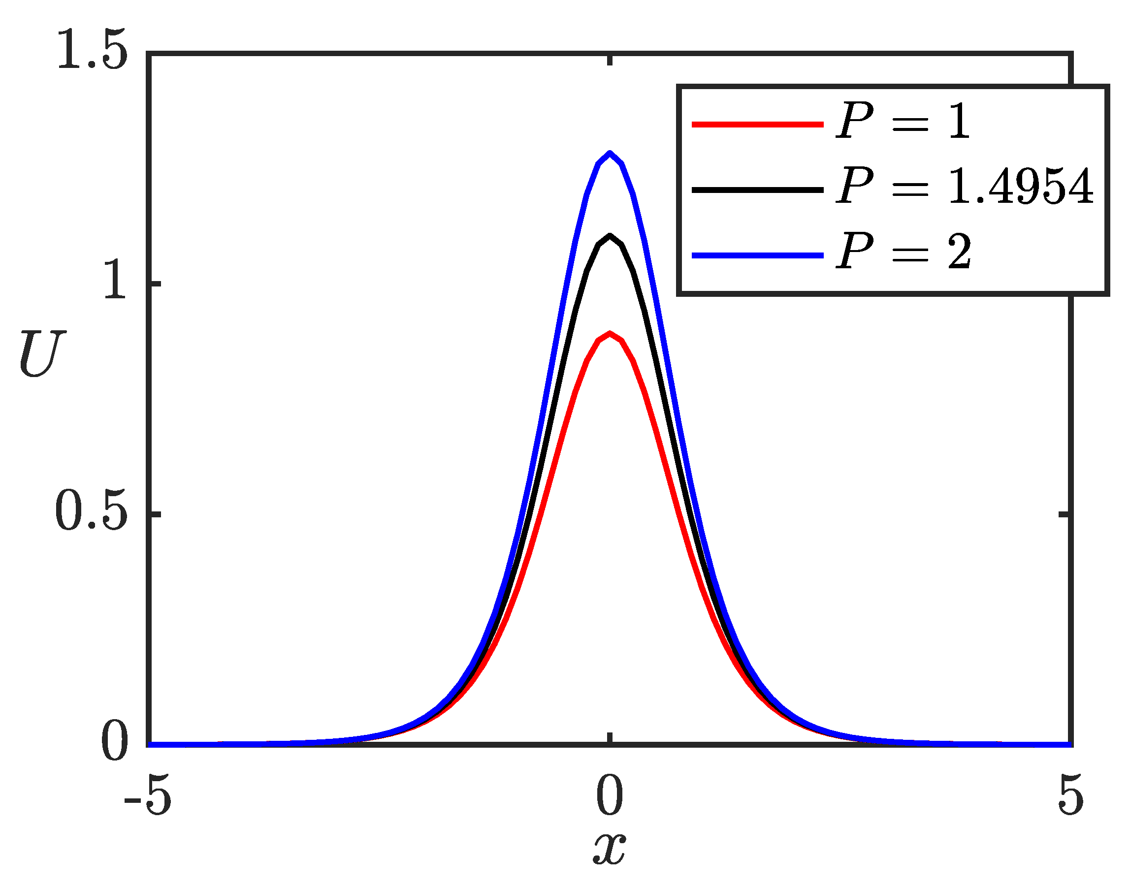
Figure 2.
Dependences for the GS families, produced by the numerical solution of Eq. (4) with , , and values of indicated in the figure ( pertains to the exact 1D soliton solution, as given by Eqs. (11) and (13)). The 1D power is calculated as , cf. Eq. (13). Above the turning points, the dashed curves, if extended towards , approach the value (see Eq. (12)) from the right.
Figure 2.
Dependences for the GS families, produced by the numerical solution of Eq. (4) with , , and values of indicated in the figure ( pertains to the exact 1D soliton solution, as given by Eqs. (11) and (13)). The 1D power is calculated as , cf. Eq. (13). Above the turning points, the dashed curves, if extended towards , approach the value (see Eq. (12)) from the right.
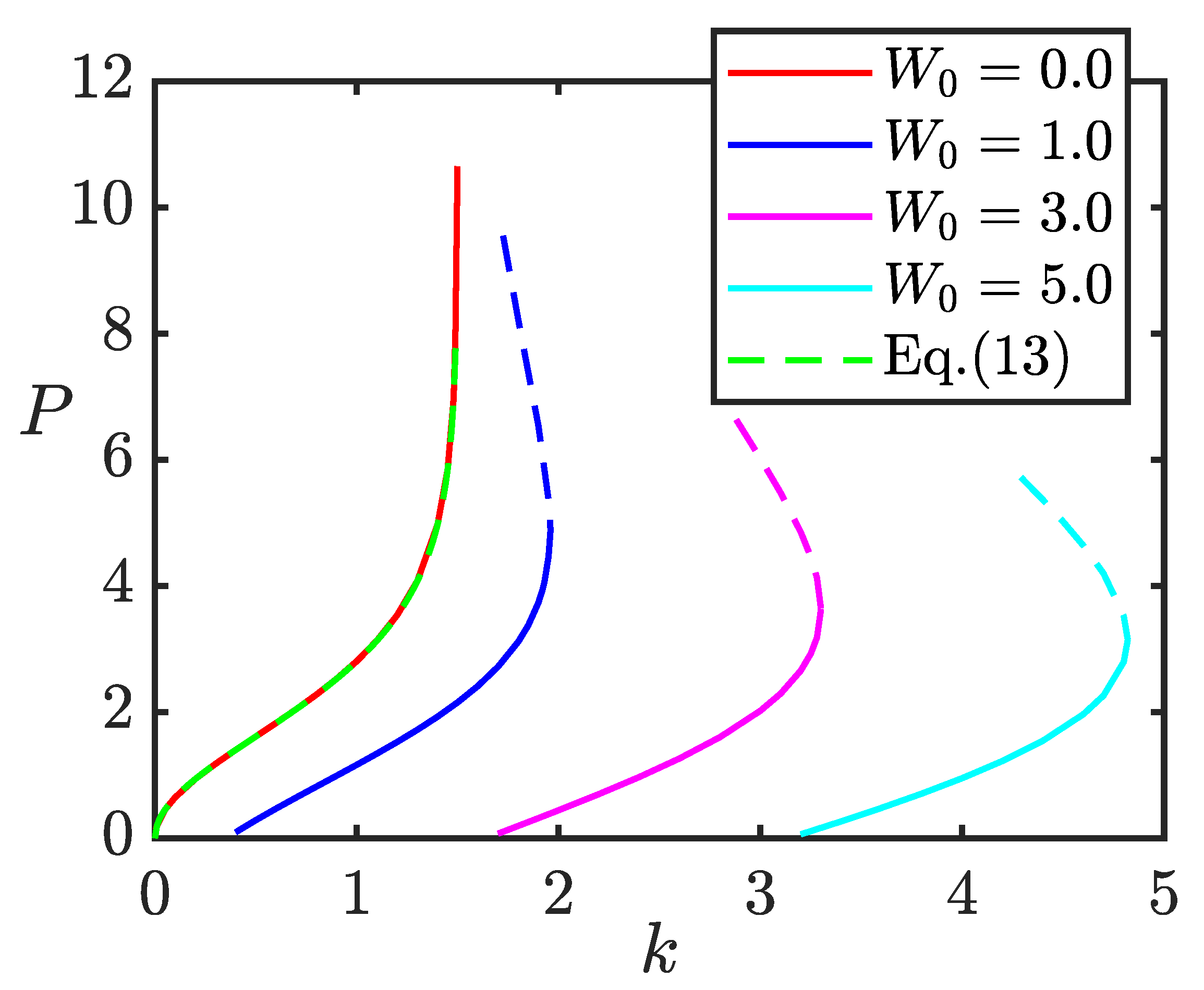
Figure 3.
The MI gain vs. wavenumber p of the modulational perturbations (see Eq. (8)) for the CW states of the GS type, with , , and different values of the 1D power, which are indicated in the figure. Note that the MI gain is vanishingly small for large powers, and .
Figure 3.
The MI gain vs. wavenumber p of the modulational perturbations (see Eq. (8)) for the CW states of the GS type, with , , and different values of the 1D power, which are indicated in the figure. Note that the MI gain is vanishingly small for large powers, and .
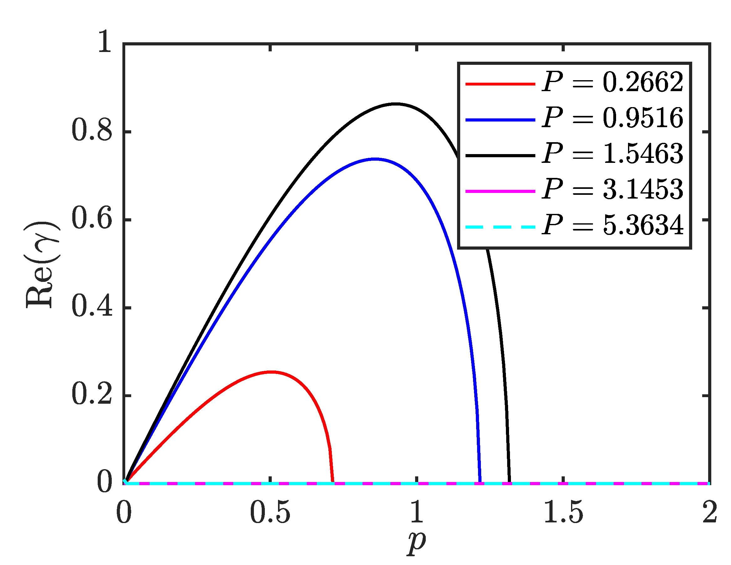
Figure 4.
The perturbed evolution of the unstable CW state corresponding to the GS profile with from Figure 1, as produced by simulations of Eq. (1). Top: the peak intensity vs. z, showing rapid growth of the MI, followed by chaotic oscillations. Middle: the local intensity, , in the -plane drawn through , showing filamentation of the CW state. Bottom: the snapshot of the power-density distribution in the plane at , which demonstrates spontaneous splitting of the unstable CW into a chain of quasi-soliton speckles.
Figure 4.
The perturbed evolution of the unstable CW state corresponding to the GS profile with from Figure 1, as produced by simulations of Eq. (1). Top: the peak intensity vs. z, showing rapid growth of the MI, followed by chaotic oscillations. Middle: the local intensity, , in the -plane drawn through , showing filamentation of the CW state. Bottom: the snapshot of the power-density distribution in the plane at , which demonstrates spontaneous splitting of the unstable CW into a chain of quasi-soliton speckles.
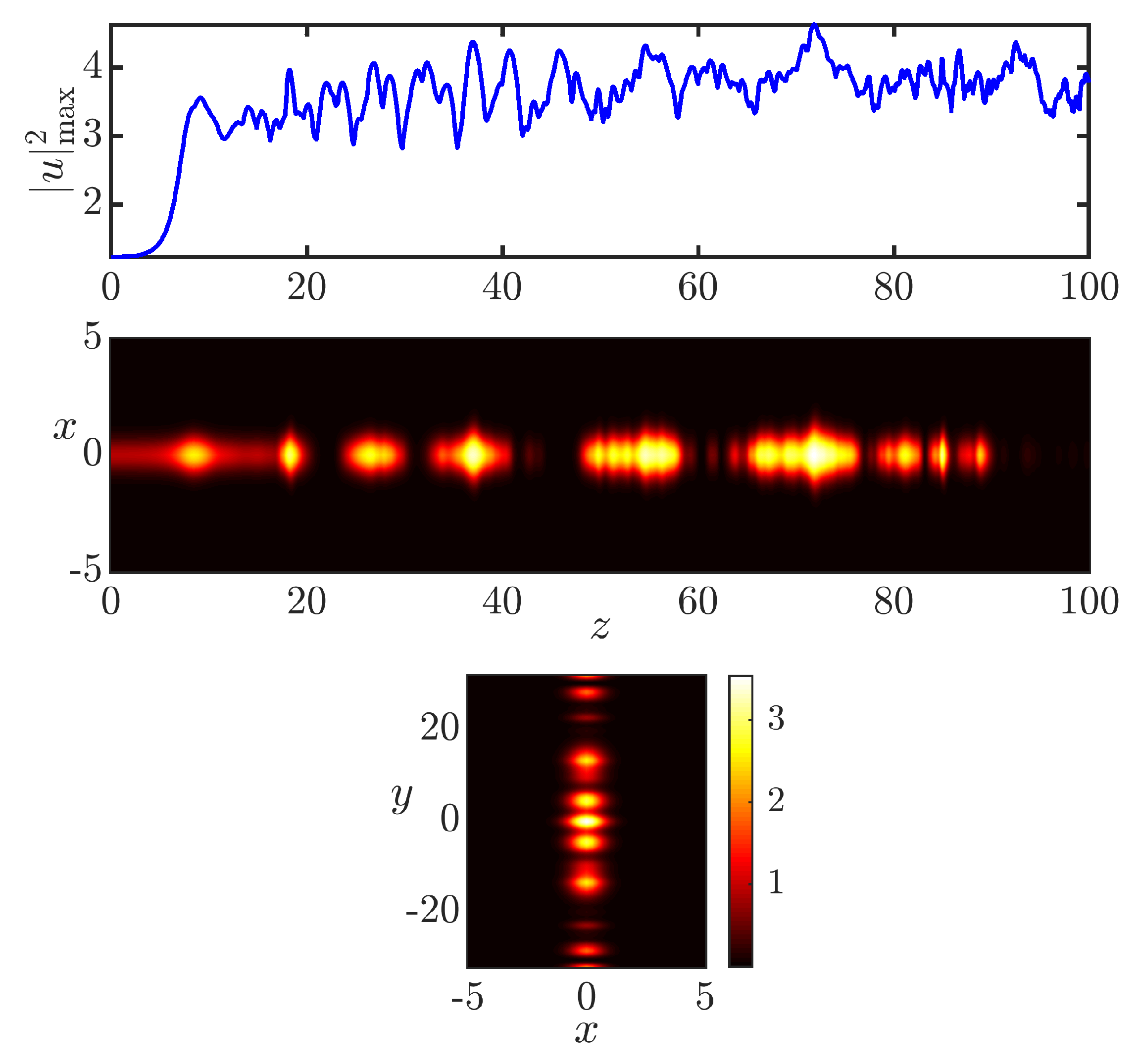
Figure 5.
The same as in the top and middle panels of Figure 2, but for a “practically stable" CW, corresponding to . and . The actual stability of this CW is explained by a very small MI gain, as obtained from the numerical solution of the BdG system of Eqs. (9) and (): .
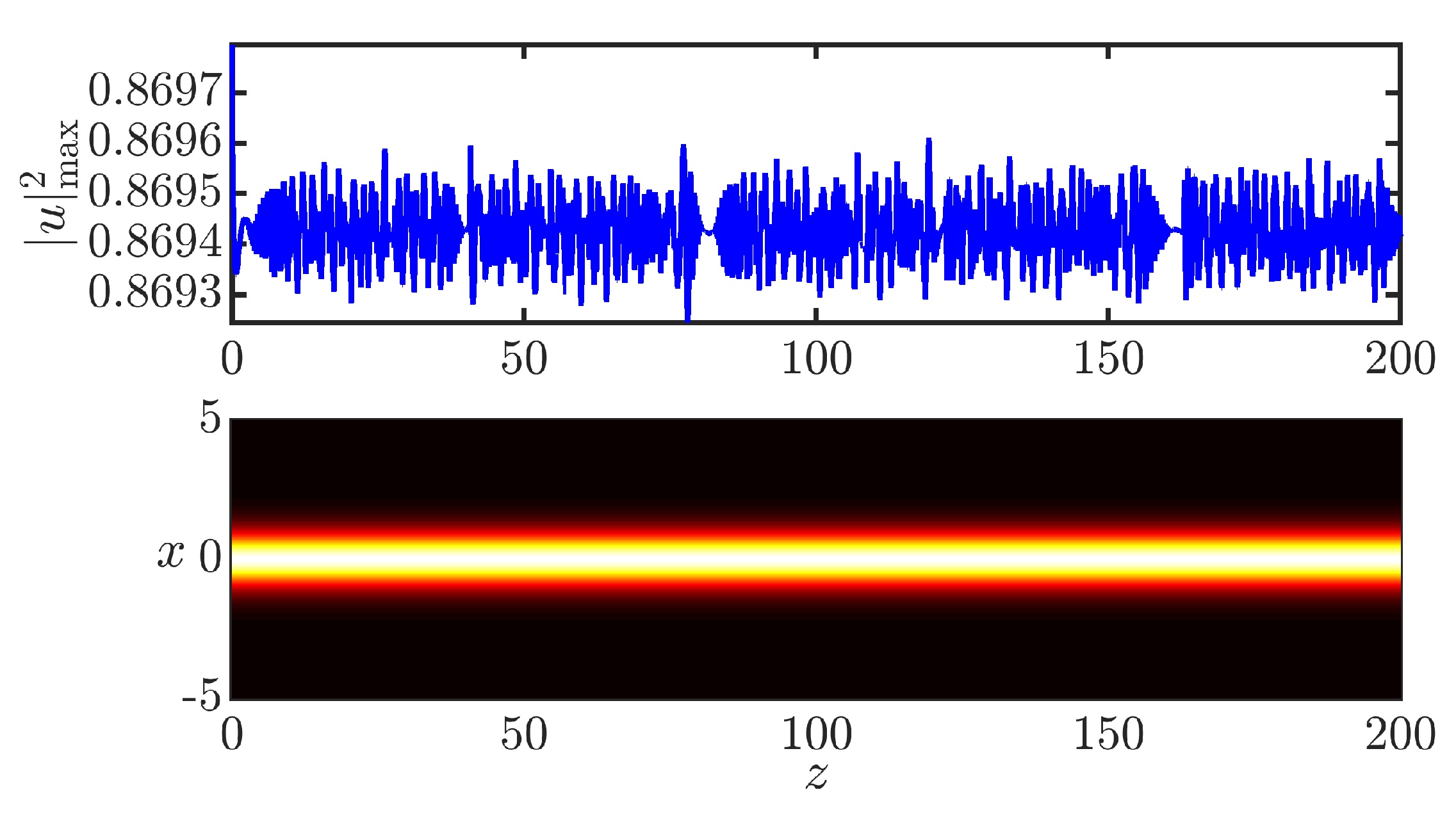
Figure 6.
(a) curves for DM families with and three values of g indicated in the panel, cf. Figure 2 for the GS modes. Circles a and b designate DM solutions for with two widely diffrent values of the 1D power, and . (b) Profiles of the solutions designated in (a). (c) The MI gain vs. wavenumber p of the modulational perturbations (see Eq. (8)) for the same CW solutions which are designated in panel (a) and presented in (b).
Figure 6.
(a) curves for DM families with and three values of g indicated in the panel, cf. Figure 2 for the GS modes. Circles a and b designate DM solutions for with two widely diffrent values of the 1D power, and . (b) Profiles of the solutions designated in (a). (c) The MI gain vs. wavenumber p of the modulational perturbations (see Eq. (8)) for the same CW solutions which are designated in panel (a) and presented in (b).
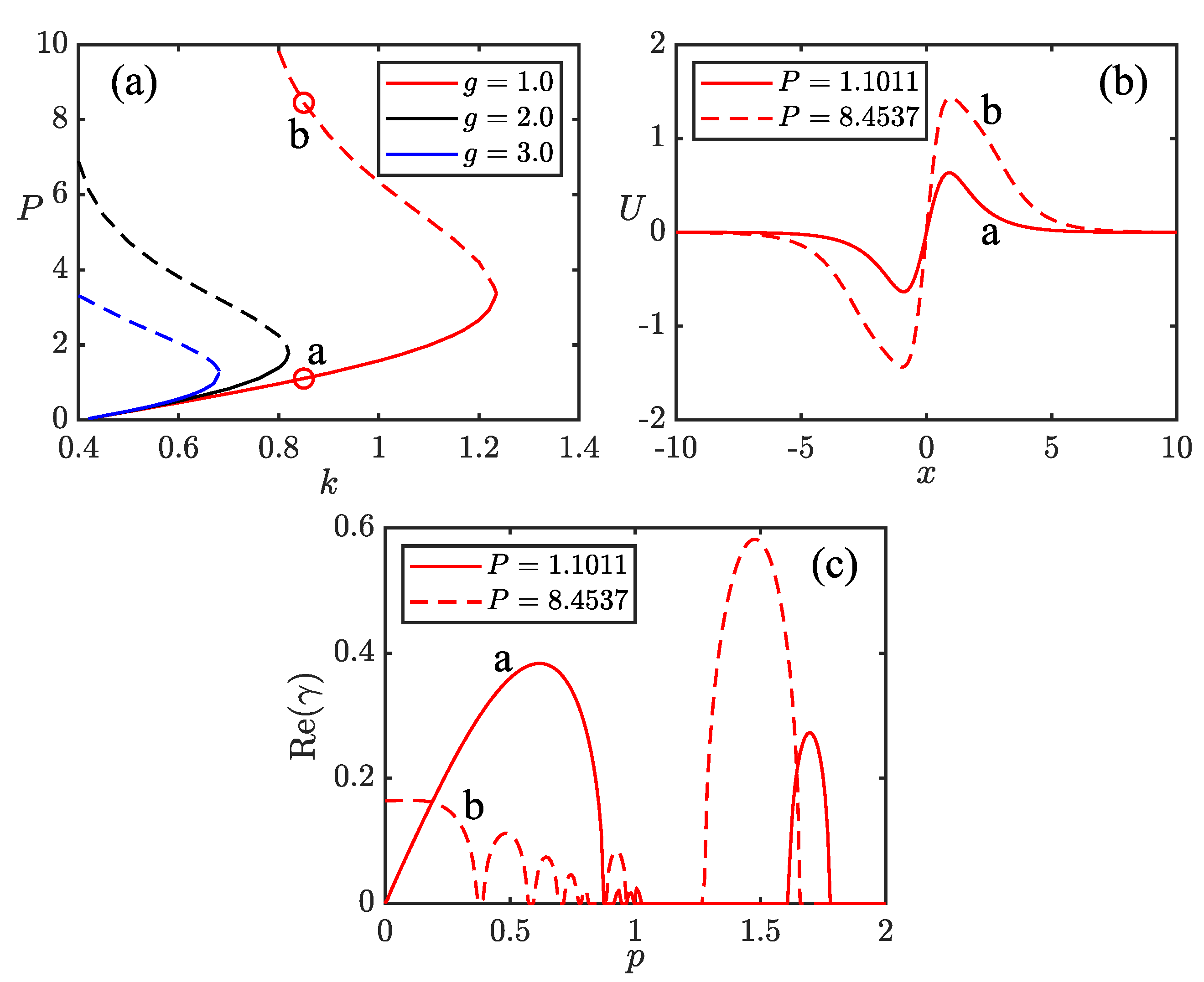
Figure 7.
The same as in the top and middle panels of Figure 4, but for the perturbed evolution of the CW of the DM types, in the case of , . and , the corresponding propagation constant being For this CW state, the MI gain is , attained at the wavenumber of the modulational perturbation , see Eq. (8).
Figure 7.
The same as in the top and middle panels of Figure 4, but for the perturbed evolution of the CW of the DM types, in the case of , . and , the corresponding propagation constant being For this CW state, the MI gain is , attained at the wavenumber of the modulational perturbation , see Eq. (8).
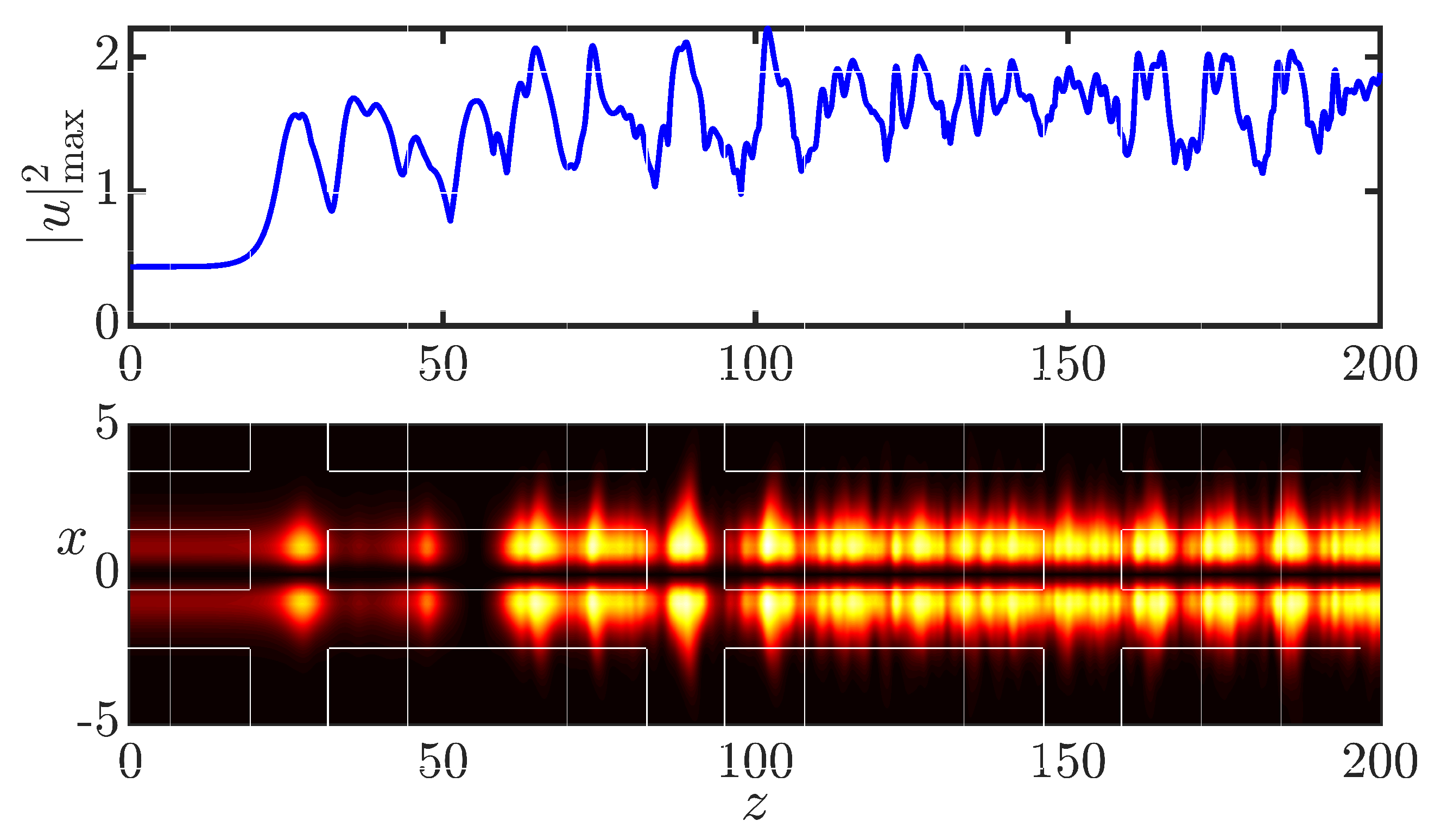
Figure 8.
The same as in Figure 7, but for the perturbed evolution of the “practically stable" CW of the DM type, in the case of , , and (the same value of P as in Fig. Figure 7), he corresponding propagation constant being For this CW state, the MI gain is , attained at the wavenumber of the modulational perturbation , see Eq. (8).
Figure 8.
The same as in Figure 7, but for the perturbed evolution of the “practically stable" CW of the DM type, in the case of , , and (the same value of P as in Fig. Figure 7), he corresponding propagation constant being For this CW state, the MI gain is , attained at the wavenumber of the modulational perturbation , see Eq. (8).
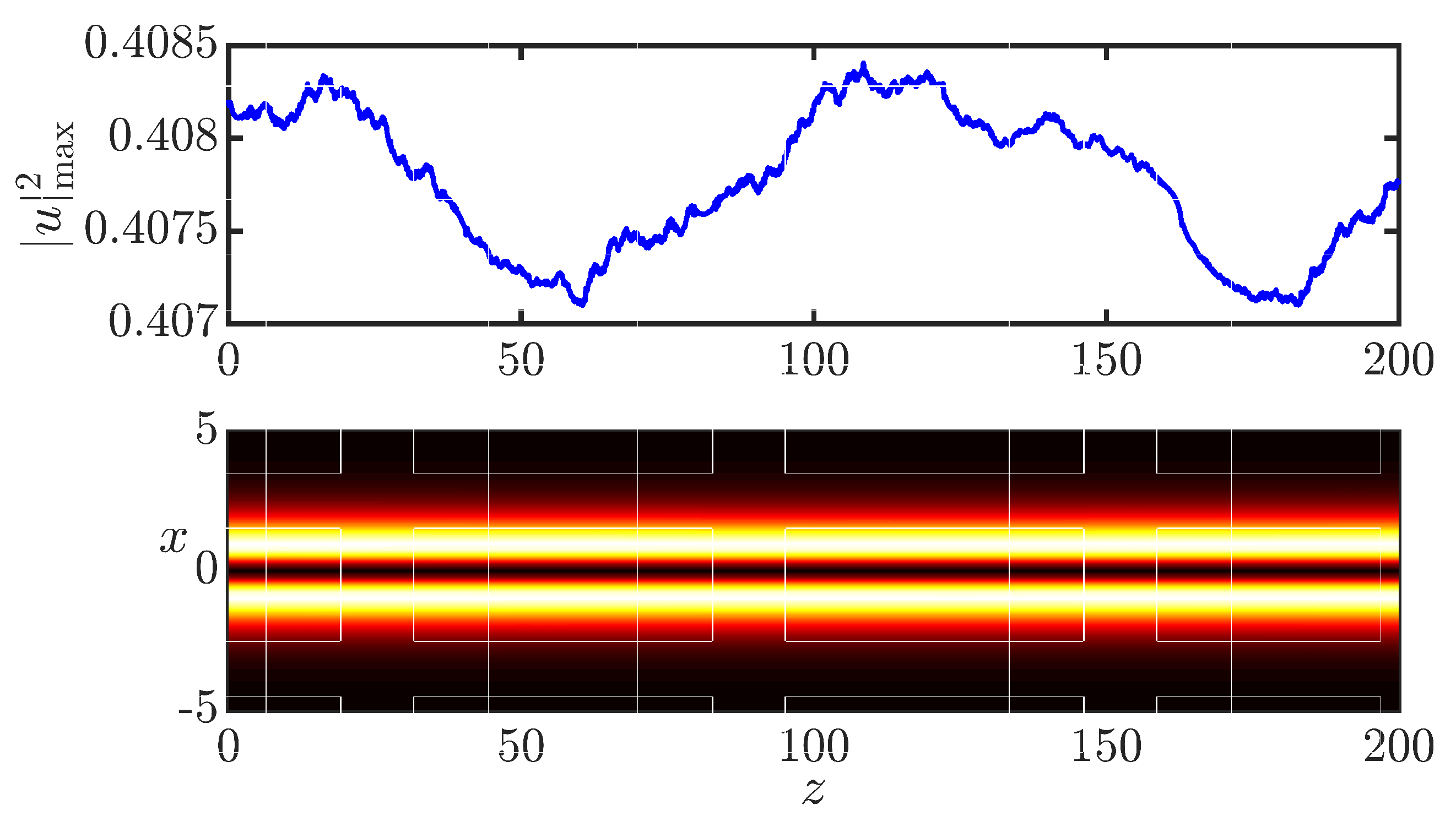
Figure 9.
Two-dimensional power P of the stationary soliton-chain solutions vs. the propagation constant k, as produced by the numerical solution of Eq. (15), with the turning point at . The family is stable, except for the red-dashed part at small values of k and large P. Markers (a) and (b) indicate the representative solutions, with and , respectively, which are displayed in Figure 10.
Figure 9.
Two-dimensional power P of the stationary soliton-chain solutions vs. the propagation constant k, as produced by the numerical solution of Eq. (15), with the turning point at . The family is stable, except for the red-dashed part at small values of k and large P. Markers (a) and (b) indicate the representative solutions, with and , respectively, which are displayed in Figure 10.
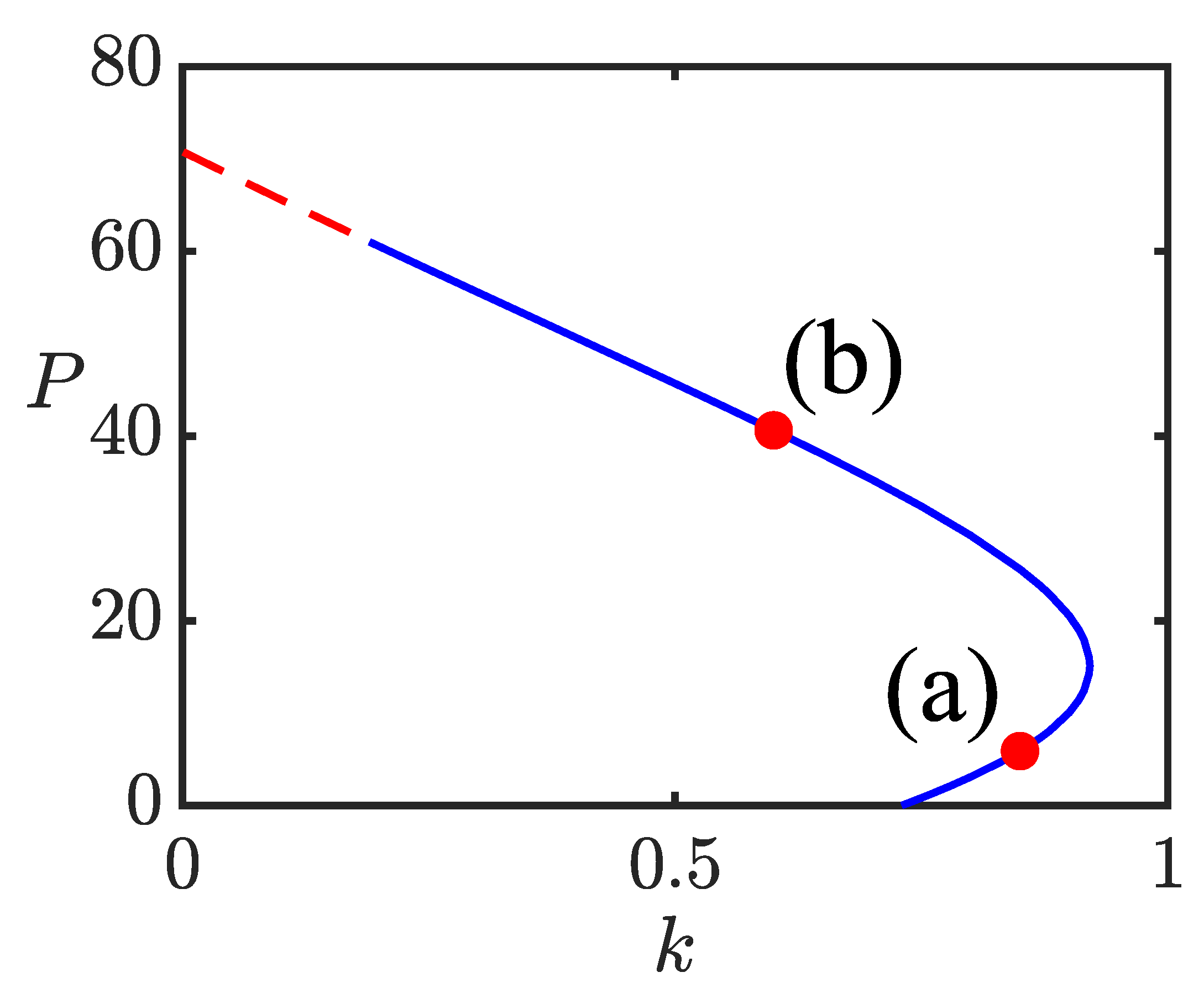
Figure 10.
Examples of stable soliton-chain solutions, labeled by (a) and (b) in Figure 9. In panels (a) and (b) the solutions correspond to the propagation constant, total power, and amplitude , , and , , , respectively.
Figure 10.
Examples of stable soliton-chain solutions, labeled by (a) and (b) in Figure 9. In panels (a) and (b) the solutions correspond to the propagation constant, total power, and amplitude , , and , , , respectively.
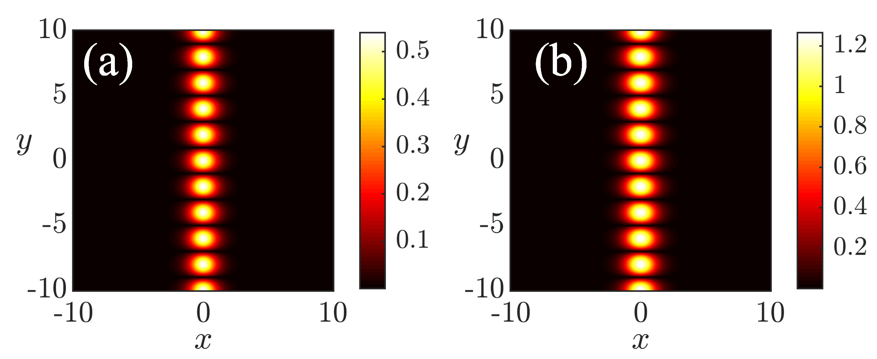
Figure 11.
The response of the soliton chain, whose stationary form, with and , is plotted in Figure 10(b), to the localized kick applied in the y direction, as per Eq. (17) with . Top: the evolution of the local intensity in the cross-section . Middle: the evolution of in the cross-section ; the cyan circle marks the location of the kicked soliton. Bottom: the evolution of the phase of in the cross section .
Figure 11.
The response of the soliton chain, whose stationary form, with and , is plotted in Figure 10(b), to the localized kick applied in the y direction, as per Eq. (17) with . Top: the evolution of the local intensity in the cross-section . Middle: the evolution of in the cross-section ; the cyan circle marks the location of the kicked soliton. Bottom: the evolution of the phase of in the cross section .
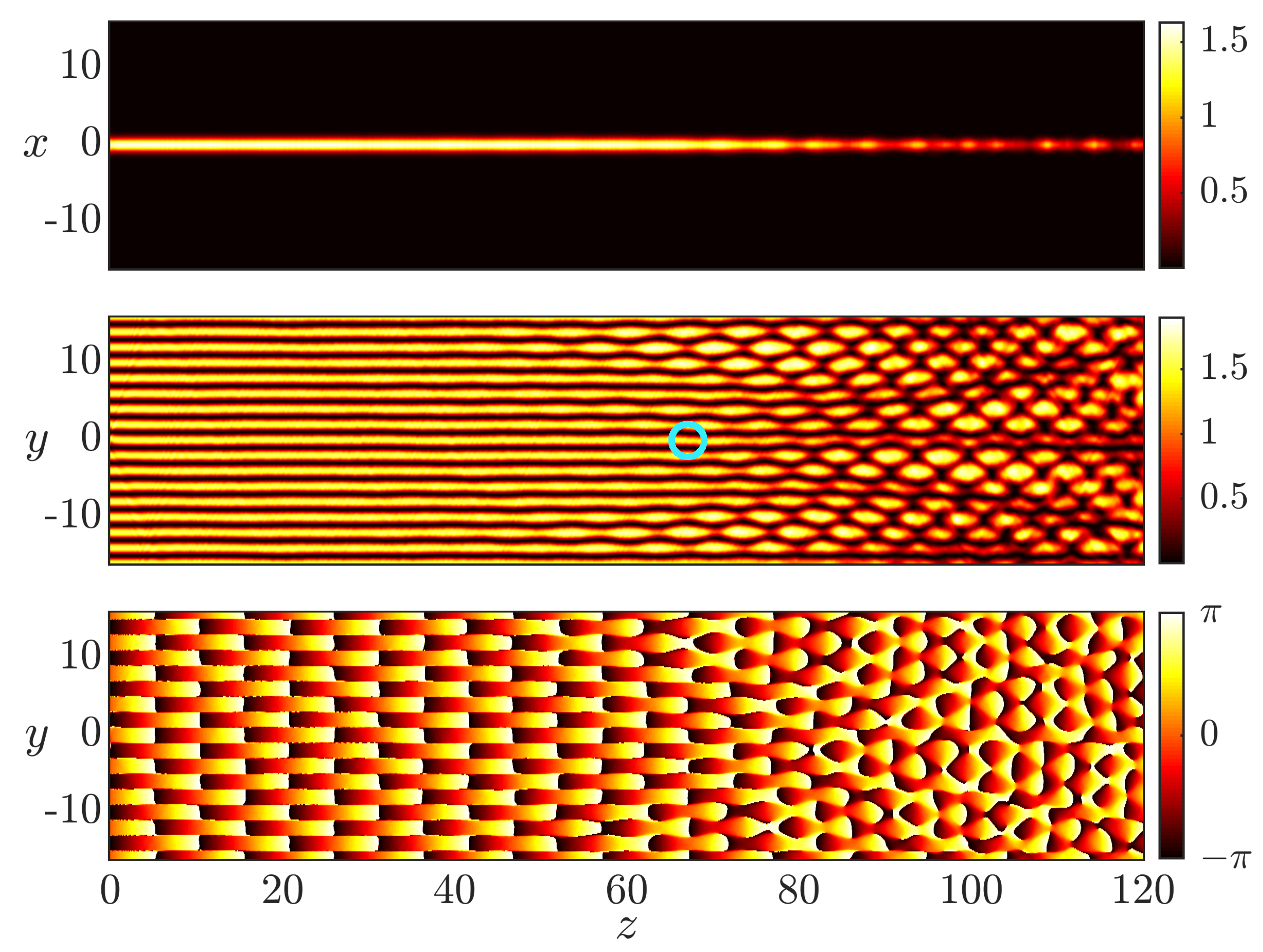
Figure 12.
The same as in Figure 11, but for the localized kick applied in the x-direction, as per Eq. (19) with .
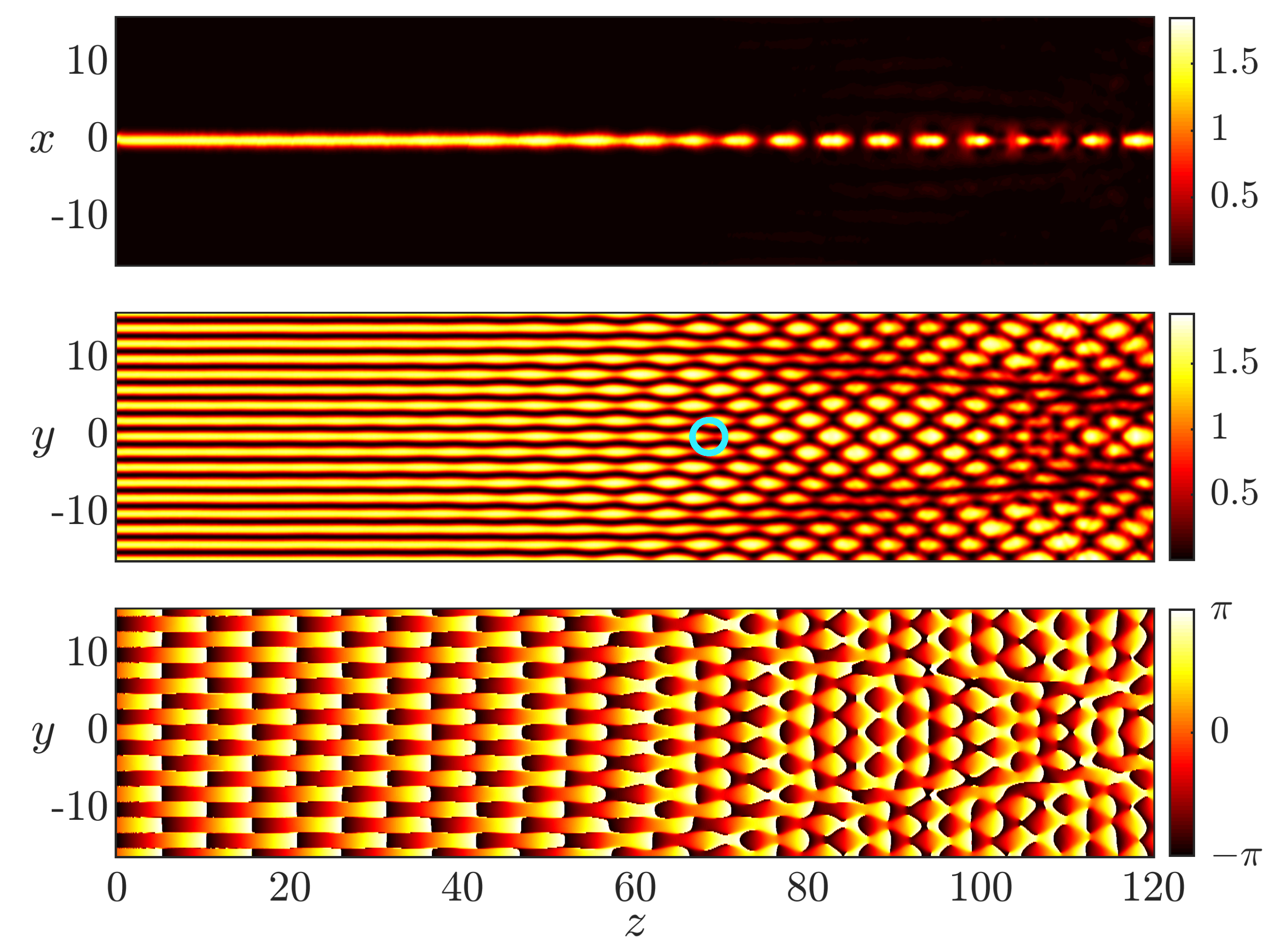
Figure 15.
The family of the transverse CW profiles, produced by Eq. (20), with , which corresponds to Case 2, in terms of Eq. (6). The family is represented by the dependence of the 1D power P on k. The dashed red curve shows the result generated by the integration of the exact solution (29), while the chain of circles shows the values of the power for the numerically found solutions.
Figure 15.
The family of the transverse CW profiles, produced by Eq. (20), with , which corresponds to Case 2, in terms of Eq. (6). The family is represented by the dependence of the 1D power P on k. The dashed red curve shows the result generated by the integration of the exact solution (29), while the chain of circles shows the values of the power for the numerically found solutions.
Disclaimer/Publisher’s Note: The statements, opinions and data contained in all publications are solely those of the individual author(s) and contributor(s) and not of MDPI and/or the editor(s). MDPI and/or the editor(s) disclaim responsibility for any injury to people or property resulting from any ideas, methods, instructions or products referred to in the content. |
© 2026 by the authors. Licensee MDPI, Basel, Switzerland. This article is an open access article distributed under the terms and conditions of the Creative Commons Attribution (CC BY) license.
Copyright: This open access article is published under a Creative Commons CC BY 4.0 license, which permit the free download, distribution, and reuse, provided that the author and preprint are cited in any reuse.