
Submitted:
26 May 2026
Posted:
27 May 2026
You are already at the latest version
Abstract
The Tomarrazón-Camarones River (La Guajira, Colombia) is characterized by frequent, widespread flooding and, anthropogenically, by intense instream sediment mining. Mapping flood hazard is hence essential to develop effective flood management plans; and a knowledge of the water regime (duration curves) is also essential to estimate sediment transport and carry out sediment budgets to inform on the impacts and sus-tainability of the mining activity. However, neither water levels nor discharges are monitored by official gauging stations, and only a few rainfall gauging stations are available in the area, with daily records often affected by data gaps. Therefore, a first challenge is to reconstruct flowrate time series by an affordable effort, scaled to the fi-nancial-labor resources available in that challenging context. This paper presents an integrated approach that combines satellite-derived rainfall data with ground observa-tions. A semi-distributed hydrological model (HEC-HMS) is used to reconstruct the full flow-rate time series once calibrated and validated with data derived from automatic sensors and field measurements. The model is fed with hourly data derived from daily data at ground gauging stations temporally downscaled by adopting the spatially dis-tributed hourly rainfall patterns obtained from satellite records. Before that, observed water levels in three stations equipped with water level sensors are to be traduced into discharge time series using analytical relationships based on field-measured geometric and physical characteristics. Then, these event-based hydrographs are used to calibrate and validate the model. Results show good agreement with observations, supporting a reasonable confidence in the approach. The calibrated model is then applied to long term datasets to retrieve duration curves and return periods of peak discharges.
Keywords:
rainfall-runoff modelling
; satellite rainfall data
; calibration-validation
; tropical hydrology
; Colombia
1. Introduction
Globally, only a small fraction of the world’s watersheds is gauged, and extreme flood prediction in ungauged catchments remains one of the main challenges of hydrology [1]. In many areas of the Global South, particularly in the tropics, a lack of hydro-meteorological data remains a significant issue [2]. In these regions, official gauging stations for discharge -and even more for sediment transport- are quite infrequent, and rainfall records are often inconsistent and usually provided on a daily basis [3]. In tropical regions such as the Caribbean and northern South America, this problem is further intensified by intense rainfall or real extreme precipitations. Indices in Colombia show spatially scattered, but statistically significant long-term increasing trends of intense precipitations [4], translating directly into greater flood hazard in catchments that remain largely ungauged.
Consequently, data gaps, measurement uncertainties, and the need for careful synthesis of hydrological relationships (e.g., stage–discharge curves) must be addressed [5], in order to approach hydrological analyses and water-related management planning. These issues are even more severe in small- to medium-sized tropical basins, like the one we considered (about 500 km2 ), where heavy convective rainfall can cause flashy hydrological responses with severe damages [6] and imply the need of sub daily time scale analysis (typically, hourly or less). In this context, satellite-derived precipitation products offer a promising potential solution to the problem of data scarcity.
Over the last few years, hydrological studies using satellite-based precipitation datasets have indeed increased. The most common products include CMORPH, TRMM, and GSMaP [7,8,9], as well as IMERG [10] and reanalysis products like ERA5 and ERA5-Land [11]. Despite considerable improvements in spatial and temporal resolution, these datasets, unfortunately, still suffer from uncertainties. In particular, satellite-based precipitation amounts and intensities may not always be reliable when used as inputs for hydrological modelling [12,13]. However, worldwide recent studies have specifically evaluated satellite precipitation products in data-scarce or ungauged basins using hydrological models with good performances. In the sparsely gauged Chenab River basin in Pakistan [14], IMERG, GSMaP and CHIRPS provided useful flood simulations, with GSMaP performing best after simple local calibration and bias correction. In the Blue Nile basin in Ethiopia [15], bias-corrected IMERG, GSMaP and PERSIANN enabled near-real-time flood modelling in poorly gauged regions. Similarly [16], analyzing several West African catchments and integrating soil moisture information with IMERG-based satellite rainfall products, showed improved daily river flow prediction compared to the standalone GPM product as well as gauge- and reanalysis-based datasets. Also [13,17,18] have shown that high-resolution IMERG products perform well, making them promising options for hydrological applications in areas with scarce data. Nevertheless, satellite rainfall products can also contain significant biases particularly in tropical regions. According to the review of [19], satellite precipitation products exhibit significant location-dependent biases, with PERSIANN overestimating light precipitation (<5 mm) in equatorial areas and CMORPH overestimating precipitation over tropical basins. More broadly [20], confirmed that bias in satellite precipitation products represents a major issue across several basins worldwide, with model performance strongly dependent on topography, seasonality, and precipitation type. Bias correction methods are hence seen as necessary to reduce streamflow errors.
Field measurements are therefore clearly crucial for calibrating and validating hydrological models, even when remote-sensing products like digital terrain models (DTMs) and land-use datasets are available. In-situ surveys allow indeed for the in-depth characterization of river cross-sections and the development of reliable stage-discharge rating curves [21], which are essential to translate water level data into flowrate, required for calibrating and validating hydrological models [22,23].
This paper addresses the challenge to obtain a reliable information on flow rate time patterns in the Tomarrazón-Camarones Basin (La Guajira), a relatively small ungauged tropical basin in northern Colombia. Actually, the interest in this case study concerns two facets: flood risk, on the one side, and geomorphological dynamics linked to alteration of sediment transport caused by an intense sediment mining activity, on the other side. Moreover, the river is the backbone of the Santuario Fauna&Flora Los Flamencos national park, feeding the Navío Quebrado coastal Lagoon [24,25]. Hence, one of the planning priorities is estimating the transport capacity of the river and to compare it with current extraction. Consequently, we are both interested in i) flood peaks analysis and ii) in the flowrate duration curve assessment. The sediment transport issue is not developed in this paper as here we are concerned with the preparation of the basic peace of information -hydrology- to later deal with it.
The purpose of this paper is to demonstrate how the sought hydrological answers can be obtained by integrating meteorological, hydrological and topographic field measurements with satellite data. It also introduces a novel approach to modelling fast dynamic processes (hours) in regions similar to ours based on daily ground-based precipitation data, while exploiting hourly satellite data, together with automatic continuous sensors, mathematical modelling and field measurements.
Its added value is providing a replicable example that can be of help in several similar cases with scarce information.
Specific to the case study, an additional relevant added value is the supply of an information (flow rates and hydrograph shape) based on measured data which is definitely new for the Tomarrazón-Camarones basin with elements common to all basin of the Sierra Nevada de Santa Marta. Actually, since the first issue of the POMCA [26] just estimations based on hydrological similitudes were considered.
Sustainable water management is a cornerstone of the 2030 Agenda; among the greatest challenges facing this resource are data scarcity, pollution, and climate variability [27]. In regions where traditional monitoring infrastructure is insufficient, Earth Observation (EO) and remote sensing technologies are emerging as essential and cost-effective tools for closing critical information gaps and supporting water governance [27].
This study contributes to targets such as integrated water resources management (Target 6.5) and the protection of strategic ecosystems (Target 6.6) of the SDG 6 (Clean Water and Sanitation) through the use of satellite data that improves the spatial and temporal coverage of monitoring [27]. Likewise, the integration of hydrological models and remote sensing strengthens territorial resilience against extreme events, aligning with SDG 13 (Climate Action) by providing early warnings and facilitating adaptive planning in vulnerable environments [28,29]. By moving beyond the realm of research into practical applications, this study provides findings that serve as input for decision-making, contributing to the achievement of sustainable development goals.
2. Materials and Methods
2.1. Study Area and Problem Delineation
The study was conducted in the Camarones–Tomarrazón basin, on the northern flank of the Sierra Nevada de Santa Marta, La Guajira, northern Colombia (Figure 1a). This region, part of an isolated coastal massif, is quite peculiar for a number of reasons:
- tropical climate with heavy convective rainfall events exacerbated by the orographic effect with very high precipitation intensities (average monthly values ranging from about 1400 mm yr−1 in the upper basin to 700 mm yr−1 in the lower basin [2]);
- very steep mountain slopes and small size basins with flashy hydrological responses and amazing sediment supply also linked to accelerated deterioration of granite rock formations with very thick layers of regolith ready to be eroded. Indeed, most of the basins see a geological transitions from a consolidated Mesozoic basement (Jurassic granodiorites and Cretaceous ignimbrites), in the steep upper catchment, to Neogene sedimentary sequences and Quaternary alluvial-coastal deposits in the lower plains [2,3,4];
- piedmont river stretches highly dynamic, with alluvial-fan development, high lateral channel mobility and large alluvial deposits [2] (Figure 2b) where typically infiltration losses occur that feed the underlying aquifers;
- impressive deforestation legacy (“marimba” period from the seventies golden age of marijuana):
- generalized indigenous population;
- widespread socio-political problems which make hazardous the access to the river and pose challenges to the conservation of any device and sometimes to the life of researchers.
As anticipated, the communities within the Tomarrazón-Camarones Basin, are affected by two interlinked problems: i) flooding (expected to grow with climate change); and ii) fluvial dynamics effects like bank erosion, incision and avulsions also foreseen to worsen because of climate change, but apparently strongly linked to instream sediment mining. Sediment mining is an extremely important and growing issue in Latin America (LA) and many other countries, including important heavy metals pollution issues [30]. In this basin (Figure 3) this activity has been going on for 40 years with a high volume of daily extraction. The miners are currently trying to achieve the status of artisanal workers which would grant them an environmental license.
However, no hydrological stations were present in the basin (and no sediment transport data has ever been collected) before our project. Although there is a river basin management plan (which recognizes this issue amongst others), no specific studies are available.
The research question of this study was hence whether it would be possible to collect field data that enabled the estimation of flood peaks and duration curves from direct measurements within the basin, rather than through hydrological similitude approaches based on data from the few gauged basins available in the region. The research hypothesis was that the lack of high temporal resolution rainfall data can be compensated by satellite data, and that estimating flow rates using low-cost devices in such a hostile environment is a feasible goal.
2.2. Methodology
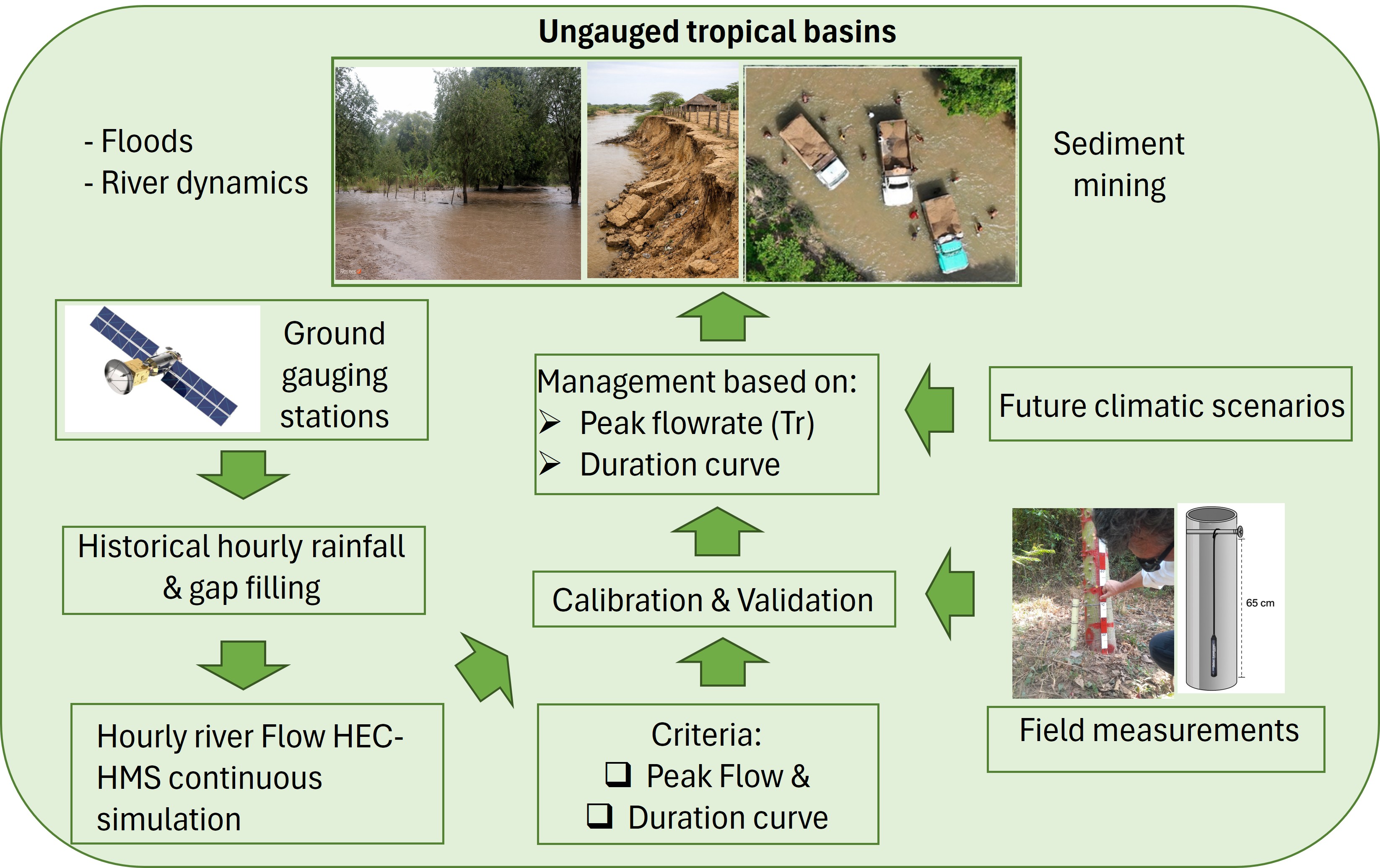
The methodology adopted is represented in Figure 4 where the red frame denotes the expected outputs. The different parts (boxes) are explained in what follows. The figure is quite dense and can be fully appreciated after reading the whole paper, but it serves as a thorough reference and for that reason is offered here. As a synthesis, high-resolution IMERG rainfall data are used to derive hourly precipitation patterns to disaggregate daily ground-based observations. Water level measurements collected at multiple river cross-sections are converted into discharge time series using an articulate procedure based on field data. These time series are then employed to calibrate and validate an hourly HEC-HMS semi-distributed hydrological model by looking at its performance in terms of both flood peaks and duration curve reproduction. The model is eventually applied to the full historical record of precipitations to derive discharge return periods.
A number of candidate stations were selected which complied with a number of criteria, both technical (hydraulic uniformity: straight reach, no islands or trees or rocky outcrops, representativity of a whole reach, covering the area of interest: basically the middle-high to low part of the basin); and practical: accessibility (often the vegetation or other natural impediments prevent one to get to the river), safety (enclosed in a private property to reduce the risk of vandalism), and possibly limited anthropogenic activity. In each one of the three selected stations we installed a sensor of water level: in station B we adopted a commercial sensor (Sonlist Levelogger LT 5) for water depth (that is a pressure sensor to be complemented by an external barometer installed elsewhere, in a safe place, but not too far apart), while in station A and C, an Arduino self-made sensor for water height was adopted. This latter was hung from a robust branch of a nearby big tree leaning towards the river and needed a complementary solar panel as energy source (Figure 5 and Figure 6).
The time series s(t) from the sensor is translated into water depth by using simple geometric relationships (Figure 7 left shows a case for the Sonlist sensor). A complication derives from the fact that, in some sections, the cross section where the hydrometer is located does not coincide with the cross section where the sensor is located. The reason is that the hydrometer must be located in a place such that an operator during flood can easily and safely see it (even without getting exactly there) and take a picture from which it is possible to read the value; but the sensor may attract thieves (there are so many people in deep need that any device may look a rewarding prey) and because of this, it has to be located in a less visible (accessible) section, possibly within a private property that, to some extent, has a better chance of survival (indeed one of our solar panels was stolen…). Therefore, there is need to first transform the sensor readings s(t) into water depth h” (t) values at that same section and then transform these latter values into the corresponding values h(t) at the hydrometer section located a distance L apart (a similar discourse holds for water elevation y” measured from the reference zero of the hydrometer to the water surface, or H”, the distance from the zero down to the bed bottom). Indeed, it is here that the geometric relationships like area A vs water depth h (A(h)) and the flowrate Q are determined. Notice that L is generally relatively short (< 150 m). This transfer of variables is executed as depicted in Figure 7 and Equation 3.1. An analogous transfer occurs in the reverse direction when the measurements at the hydrographs are translated into values at the sensor section in order to calibrate it.
A further complication occurs when, for several causes (e.g., a large flood), sometime after installation it may be necessary to move the sensor in a new section not coinciding with the hydrometer and hence a correspondence rule has to be used.
The translation is basically expressed by Equation 3.1 for the Sonlist case. An analogous relationship, not reported here, holds for the Arduino case.
This rule depends on the height difference Δy(Q) which in turn depends on the flowrate Q which is initially unknown and varying. As there was no possibility to actually measure it during a flood (mainly because floods occur by night and are flashy), we assumed it equal to a fixed figure Δy* measured on the field for a regular flow condition we could capture (Equation 3.1d), although we are aware that this is most probably an underestimate and certainly a source of noisy data (the equation is written to translate hydrometer data into data at the sensor section, but can be reversed):
where:
h” = H” + K + s (K < 0)
y” = y - Δy(Q) (y < 0)
h” = h - Δy(Q) + (H”- H)
Δy(Q) ≅ Δy*
H, H” [m]: depth of river bed with respect to the hydrometer conventional zero (m) in the original (hydrometer) and sensor sections, respectively
K [m]: (positive or negative) vertical distance from conventional zero to Sonlist sensor (m) in the sensor sections
s [m]: water height measured by the sensor (m) in its section
h, h” [m]: water depth at the original and sensor sections, respectively
y, y” [m]: water elevation, i.e., (positive or negative) segment length from the hydrometer conventional zero to the water surface, at the original and sensor sections, respectively.
Δy(Q) [m]: height difference between water surface in section hydrometer and sensor.
The time series of the variable s(t) measured by a sensor (be it water depth, in the Sonlist case, or distance to water, in the Arduino case) has to be transformed into a time series h(t) of water depth. Even in the Sonlist case, s(t) does not coincide with h(t) for a number of reason: the first one is that the zero of the sensor does not coincide in general with the bottom of the river, because the sensor has to be somehow protected (or not fully exposed) from the river current, so it is generally anchored to a robust support on the bank (typically a tree or a big root); furthermore, our transformation relationships (Equation 3.1) include some assumptions (the constancy of Δy(Q) that, theoretically, in very harsh and flashy events might even change sign, although this is not the case in our situation) and, in addition, the maximum distance H between the reference zero of the hydrograph and the deepest point of the river bed cross section may change in time owing to hydrodynamic processes; finally, there may be some error in coupling the levelogger sensor to the barometric sensor (the needed data is indeed the difference). In addition to these static causes of error, there may also be a mismatching between the sensor clock and the time measured on the field.
Because of these reasons, a calibration is necessary, and consists in applying a delay correction and a vertical correction; this latter is obtained by moving the curve to fit the few measurements taken in the field during flood events. So far, however, a true flood peak has not been captured during our field visits -while it has by sensors- because the hydrograms are very sharp and short (approximately 6 hours between the rising and falling limbs) and floods typically occur at night; field surveys are usually conducted in the early morning following intense rainfall, allowing only the falling limb of the event to be captured.
An example of calibration procedure is shown in Figure 8. Notice that in general an important additional criterion is to ensure a consistency in the time sequence of events recorded at stations located along the river: the downstream station must see the event after a reasonable time shift representing the flood travel time. In addition, any vertical or delay adjustment must be applied for all flood events belonging to a same “morpho-period”, that is an interval of time enclosed between moments when a significant morphological change of the reach occurred, owing either to a flood or to anthropogenic causes like sediment mining. This means that the “optimization” needs to take into account all events at a time.
Notice that there are no data outside the flood event period, as the sensor is not located at the bottom of the river because it would be impossible to ensure its stability and would be very vulnerable to woody debris and sedimentation; as a matter of fact, therefore, it can only capture events with water levels higher than the threshold H- K of Figure 6; the rest of the time is hence blank (no data).
Discharge was estimated simply by the following Equation 3.2:
where:
Q* = v* A*
Q(t) = v(h(t)) A(h(t))
v: velocity (m/s)
A: wetted area (m2)
*: denotes a field measurement at a time ti
v(h): denotes an analytical relationship between the velocity and the water depth, built by interpolating and extrapolating, for higher flows, via Manning equation the field measurements obtained
A(h): analogously indicated an analytical relationship built on the geometry of the section surveyed on the field (Figure 9).
The velocity v* was estimated by measuring the displacement time Δt of a floating object between two fixed sections of known distance ΔL: v* = ΔL/Δt (taking the average of at least three runs). Again, there was no possibility to make a true discharge measurement by human driven devices, like velocity meters or ADCP, because there is no possibility to be physically there during the event. A night vision video camera might serve the purpose, but was outside the possibilities of the project.
It has to be noted that particularly the relationships v(h) are the weakest elements in this chain of calculations as, again, we could not get (yet) a real measurement during a peak flow. Therefore, values have been extrapolated based on Manning hydraulic equation (fitted on the low-medium values available).
A dynamic relationship (hydrological model) between rainfall and flowrate is needed because of two reasons at least:
a- to determine the duration curve and, with that, estimate the expected sediment transport during the project period and, then, during the average historical hydrology, provided that a calibrated sediment transport formula be available (this is the object of another forthcoming paper). With that, it is possible to address key questions related to sediment mining like comparing extraction with supply and perform a sediment budget to investigate the effect on river morphology;
b- to estimate the flowrate Q(TR) associated with different return period TR, and hence derive flood maps to guide land use planning. This implies reconstructing the whole historical regime.
Precipitation
To feed this model, precipitation time series are needed. Unfortunately, there only are 4 gauging IDEAM stations in the basin and around, and they only collect daily data, while, as is apparent from Figure 8 above, the basin is flashy and an appropriate time step must be no longer than an hour. This statement can be rigorously derived from Shannon’s theorem about data sampling [33], but can more practically be inferred by just observing the hydrographs from which a significant change of water level (or flowrate) is already visible after an interval of less than one hour.
To overcome this limitation, satellite-based precipitation data from the GPM IMERG Final Run V07 product [34], with a spatial resolution of approximately 10 km and a temporal resolution of 30 minutes (2014–2023), were accessed via Google Earth Engine (Table 1). IMERG precipitation data were extracted from the grid cells corresponding to the geographic locations of the four meteorological stations operated by IDEAM (Figure 1). The extracted time series were subsequently processed in RStudio (version 2023.03.0 Build 386). For each month of the year, precipitation events were analyzed to derive typical intra-daily rainfall distributions. Hourly precipitation was computed from the 30-min GPM IMERG data by temporal aggregation, and the relative contribution of each hour to the total daily rainfall was calculated. These hourly patterns were then used to disaggregate the daily rainfall data recorded at the four meteorological stations operated by IDEAM (Figure 1).
Therefore, IMERG data were primarily used to:
Two models were implemented. The first reproduced the field-measured hydrographs of seven non-consecutive events monitored during our campaigns so far, while the second employed historical IDEAM data (1973–2024) to estimate peak discharges corresponding to different return periods (TR). Daily IDEAM data were disaggregated to hourly resolution using the information obtained by the IMERG analysis, enabling the reconstruction of sub-daily hydrographs.
The semi-distributed model was implemented by using the HEC-HMS software, applying the SCS-Curve Number (CN) method to estimate direct runoff. Initial abstraction (Ia) was calculated as a fraction of the maximum retention S (Ia = 0.2 S), and soil moisture conditions were taken into account through the CN. Sub-basins were delineated according to the main tributaries and the installed monitoring stations (Figure 1, Study Area). Runoff transformation from excess precipitation to direct runoff was performed using the SCS Unit Hydrograph method. Baseflow contributions were represented using a recession method to account for delayed flow. Flow routing along river reaches was implemented using the Lag method, with lag times estimated from reach lengths and average channel slopes according to the standard SCS formulation:
where is the lag time (hours), is the reach length (km), is the average channel slope (m/m), and is a unique empirical coefficient calibrated based on the observed hydrographs.
Calibration and validation
Any mathematical model must be calibrated. But calibration can take different forms depending on model purpose. Here, in particular, the problem is not replicating as faithfully as possible the recorded pattern because: i) the approach adopted to tune the sensors leaves space to a certain degree of discretion concerning the delay (we found out that the Arduino clock progressively distorts time); ii) low flows were not recorded; and, more important, iii) to our purpose, the model needs to reproduce reliably the flood peaks (to then estimate flowrates associated with return periods) and the duration of different flow rates (to determine expected transport capacity). Therefore, rather than adopting the usual model performance indicators (RMSE, Nash–Sutcliffe efficiency,..), we opted for two ad hoc performance criteria, a position that gives rise to a multiobjective optimization exercise. The criteria are as follows:
- a)
- minimize the deviation on peak flows (Equation 3.3) measured by a normalized index pN(c), the lower the better. This quantifies the normalized sum of the relative deviations between simulated and observed peak flows for all flood events, given a model parametrization c. The normalization is based on the min-max across all model parametrizations considered:
pN(c) = [p(c) – min C p(c) ]/ [max C p(c) – min C p(c) ]
p(c)= sum fÎM [ QfS(c) – QfO(c) ]/QfO(c)
- b) reproduce as accurately as possible the duration curve (Equation 3.4). The accuracy is assessed by a normalized deviation index dN(c) that quantifies the overall difference between simulated and observed flow duration curves; again, the lower the better. For each flow value Qk(c) in the time series, the exceedance probability Fkx(c) is the fraction of time that the flow equals or exceeds that value; this holds for both observed (x=o) and simulated (x=s) series. The relative absolute difference between simulated and observed exceedance probabilities is hence calculated for each flow level k. The overall index d(c) is obtained by summing these differences across all flow levels k; while the final index dN(c) is obtained by applying a min-max normalization across all configurations:
dN(c) = [d(c) – min C d(c) ]/ [max C d(c) – min C d(c) ]
d(c)= sumkÎC [ abs(FkS(c) – FkO(c)) ]/ FkO(c)
where the terms have already been defined. Notice that again the temporal phase mismatching is irrelevant to this index.
To reduce over-parameterization, only two calibration parameters were introduced: Curve Number (CN) scaling factor (α) and flow loss percentage (β) between stations A and B, representing the infiltration process into the thick alluvial sediment deposit (Figure 3) that produces a substantial reduction of flow, as often occurs in piedmont areas like ours. As per the former, a base value of the Curve Number (CN) parameter spatially distributed among the sub-basins has been derived from the GCN250 dataset available in Google Earth [35], based on land use and soil type, and averaged to obtain representative values within each sub-basin; this base value is modulated according to the scaling factor α which is the first parameter.
As sensors data are available for three stations (at the time of writing), calibration is carried out on data from stations A, B, and validation on data of the downstream station C.
3. Results
The hydrograph obtained by sensors and by the calibrated and validated model (as explained below) are presented in Figure 11. Notice that the temporal mismatching, as already said, is not a particularly relevant issue in our case as indeed the calibration and validation criteria concentrate on other aspects and are insensitive to it, as explained above.
The calibration of the model is synthesized in Figure 12 where the overall performance (right) and (left) the Pareto frontier together with the selected parametrization (red dot) are identified. It can be noted that this is a first approximation as the search for a better performance can be pushed further; results however would not change significantly.
The performance related to the dataset of stations A+B, on the one side, and that of dataset of station C, adopted for validation, on the other side, are reported in Figure 13. As it is apparent, the performance is quite satisfactory in all stations, although a certain flood peaks sub estimation occurs in station C, but just for lower values. In terms of usual basic performance indicators, for the overall hydrograph reproduction, very good agreement is observed, with R2 = 0.981, RMSE = 0.0497 (RMSE_rel = 40.04%), and MAE = 0.0302 for station C. Regarding peak flows, the model shows slightly lower but still acceptable performance, with R2 = 0.878 and RMSE = 12.60 (relative RMSE = 26.82%, MAE = 10.97) for stations A+B, and R2 = 0.888 and RMSE = 14.12 (relative RMSE = 27.21%, MAE = 11.42) for station C. Again, a certain underestimation of flood peaks occurs in station C, mainly for lower peak values, which is consistent with the higher relative error observed for extreme events.
With the calibrated model, and the historical data set of IDEAM precipitation downscaled to hourly time step, the corresponding time series of flowrates QH(t) has been obtained; a Gumbel probability distribution has been fit and the corresponding return periods obtained as reported in Figure 14.
4. Discussion
By applying satellite data from IMERG for the disaggregation of rainfall from daily to sub-daily values, the SCS-CN HEC-HMS model [36] was able to reproduce the Tomarrazón-Camarones’s hydrological regime of the wet season 2025 (April-June) including the successfully replicate peaks of flood events. This indicates that satellite rainfall can be very useful in data-scarce convective tropical basins even if not directly used as inputs for hydrological modelling [12]. Indeed, the semi-distributed HEC-HMS implementation, combined with IMERG-derived hourly precipitation patterns, allows a more detailed reconstruction of sub-daily hydrographs than would be possible using daily station data alone, representing a valuable step forward in modeling the hydrological response of a poorly gauged, flashy tropical basins like ours.
It is worth mentioning that the SCS Curve Number method adopted is empirical and was originally developed for small- to medium-scale isolated events under typical soil moisture conditions. In this study, instead, a continuous simulation was performed, which may be questionable in the estimation of peak discharges, especially over long-term applications. Nevertheless, in our case, this limitation is more theoretical than practical because as soon as the dry season ends, the basin is subject to very frequent rainfall events (flood or not) so that the terrain remains quite humid and indeed there is an important aquifer. In any case, the System Analysis approach based on calibration-validation is the framework that tells us whether the approximation is acceptable or not. Therefore, once ascertained that the HEC-HMS model was responding quite well, we preferred to stick to it also because of its wide diffusion and simplicity, thinking of an easier dissemination of the methodology.
In addition, precipitation data were derived from rain gauge measurements, which are considered reliable for the study area. While no significant bias in total rainfall volume is expected, some uncertainty in the temporal distribution of rainfall may affect peak discharge and hydrograph shape, although total volumes remain consistent with observations.
In any case, consistently with conclusions from previous research on modelling tropical rivers (e.g., [37,38], field measurements resulted crucial to increase the reliability of results [39]. In fact, in this study, the use of data collected at several monitoring stations (A, B and C, Figure 1), both manual and automated, were essential for both the translation of water depth data into flow rate values and for the calibration and validation of the model.
In this context, the quality and reliability of field data play a central role. It is hence due to notice that these data are of three types all involving peculiar difficulties:
a) period-related geometry and morphology data like the cross-section area A vs stage h relationship A(h) (representative of the associated reach) that typically changes after each significant flood or after sediment miners operate intensely for a time: a more appropriate notation is hence A (h, period).
b) direct measurements of water depth (h) or water elevation (y) and velocity (v), which occur at some (few) instants of time, typically just after a flood is already occurred, so inevitably missing the peak. Indeed, as already noticed, in our basin, as in several others of the region, rainfall tends to occur at night [40]; Figure 10 and floods are flashy (and very dangerous), so that it is virtually impossible to be at the station and capture the peak moment or the like.
c) “continuous” (actually discrete with a fine time step of one hour in our case) water depth related data s(t) from sensors. The procedure is to first transform s(t) into water depth h(t) data, an exercise involving the geometry of the section and the few measurements needed to calibrate the relationship (through the described process: s(t)→hs”(t)→h”(t) at the sensor section, and then h”(t)→h(t) at the hydrometer section); and then, to determine the discharge Q(t) by means of time-varying stage-discharge relationships Q(h, period) = v(h,period)*A(h,period). A weak point here is the manual correction of the delay of sensors time series which, unfortunately, is not constant as in the Arduino case it accumulates progressively as days elapse and it is not that straightforward to eliminate; furthermore, each time a manual download of data takes place (approx. every three months) a new, different bias can be introduced. The weakest point here, however, certainly is the relationship v (h, period) (Equation 3.2) because, until the time of writing, there has been no opportunity to directly measure velocity during a flood event; only low flow, or at most regular conditions, have been captured (only a permanent video camera could capture the event). This means that the values for high floods have been extrapolated by using Manning equation calibrated on the available data. This introduces a significant uncertainty because relatively small variations of velocity imply a more than proportional change of flowrate.
Perhaps the harshest difficulty in all this, although unexpected, has been the determination of the geometric features H, K and the like appearing in Figure 7 because the cross section continuously changes with time and suddenly during a flood or after miners intervene and the sensors (and K with them) sometimes had to be moved because of stability issues. Furthermore, as already explained, the cross section equipped with a sensor does not coincide with that where a hydrometer is installed and where measures are taken; hence, a further geometric translation of data from a section to another (not shown here) has to be performed which complicates things and introduces new uncertainties. Finally, it is to be clarified that a “measurement” can be: i) an actual measurement of water depth, possible only in moderate or low flows and requiring in any case a measure of the height difference between water surface and the zero of the hydrometer (not an easy exercise); ii) a reading of elevation at the installed stage, again very unlikely during floods; or most commonly iii) a photograph of the hydrometer implying a posterior interpretation to determine the water elevation. All these steps involve high uncertainties.
The surprising outcome of our whole exercise is, however, that, in spite of all this cumbersome and somehow fragile apparatus, and including the possibly questionable issue of hourly precipitation derived from satellite data and the use of HEC-HMS in a continuous simulation exercise, the model performs quite well.
In addition, a simulation with HECRAS of the hydrograph of the heaviest flood recorded so far provides a very realistic picture of the behavior along the river. But this will be discussed in another forthcoming paper.
Incidentally, it may be interesting to note that, globally, the cost of the two options (home-made Arduino power fed by a solar panel and commercial battery fed Sonlist levelogger) was similar, therefore strongly indicating to prefer to commercial solution (the Sonlist sensor is very compact and with an autonomy of 6 years! While the solar panel is particularly vulnerable to damages and robberies).
5. Conclusions
This paper presents a quite structured methodology (Figure 4), applied to the Tomarrazón case, to reconstruct hourly (or less) flowrate time series based on daily ground rainfall data, high temporal resolution water level sensor data and sporadic field surveys. In spite of the low level of technology involved by some of its steps (e.g., the field measurement of velocity), it provides a significant added value because it allows to get sufficiently reliable reconstruction of the flowrate time series in this type of flashy basins where gauging stations are partially or fully missing. Indeed, by applying satellite data from IMERG for the disaggregation of daily ground gauged rainfall data from daily to sub-daily values, the SCS-CN HEC-HMS model enabled us to satisfactorily reproduce the Tomarrazón-Camarones’s hydrological regime of the wet season 2025 (April-June).
It can be concluded that satellite rainfall can be very useful in data-scarce convective tropical basins even if not directly used as inputs for hydrological modelling. Nonetheless, also the field measurements resulted crucial for calibrating the hydrological model.
A particular important aspect is the adoption of calibration criteria explicitly focused on the intended use of the model, rather than blindly attempting to reproduce the entire time series derived from direct measurements. It should even not be discarded the option to use a different model depending on the purpose; e.g., one for reproducing peaks, and another to reproduce duration curves.
In conclusion, the study carried out represents an important result for land use planning and flood risk management in this ungauged part of La Guajira region, Colombia. In addition, the use of satellite data, field measurements, and hydrological modelling represents a transferable approach for other data-scarce catchments as well as a solid basis for future research in this catchment.
Further improvements are certainly advisable and possible. In particular, a video camera and an algorithm to derive surface velocities could help. But the impression that more technologically advanced and automatized gauging stations could be used, needs to be tamed by the awareness of Colombian local reality: the tropical vegetation is extremely vital and in a few weeks covers any clearing; large areas are not covered by mobile phone connectivity; any attractive device left in the field will rapidly find someone stealing it to obtain few dollars (if any) -and actually one of our solar panels feeding the Arduino devices has been stolen up to the time of writing-; flood periods often make it impossible to access the sites. Finally, entering the basin and moving across it always implies a risk from violent armed groups.
Author Contributions
Conceptualization, A.N.; methodology, A.N., L.M. and G.P.; field work and data preparation, F.H., Y.A., J.E. and E.O.; satellite data processing and hydrological modelling, G.P. and L.M.; paper writing A.N., L.M. and G.P.; editing, E.O.; visualization, G.P., F.H., Y.A. J.E.; supervision, A.N.; funding acquisition, L.M. and A.N. All authors have read and agreed to the published version of the manuscript.
Funding
This work was developed within the NATIVE project (sustaiNable riverscApe managemenT for resIlient riVerine communitiEs) supported by GCBC which is funded by the UK’s Department for Environment, Food and Rural Affairs working in partnership with DAI Global as the Fund Manager Lead.
Data Availability Statement
Data collected can be shared under specific request to the authors and after GCBC approval.
Acknowledgments
A kind appreciation has to be given to Mr. Edison who accompanied us in so many quite daring field campaigns. And a big thank to Eng. Lislie Zuñiga for her support in GIS elaborations.
Conflicts of Interest
The authors declare no conflicts of interest. The funders had no role in the design of the study; in the collection, analyses, or interpretation of data; in the writing of the manuscript; or in the decision to publish the results.
Abbreviations
a.s.l. – above sea level
ADCP – Acoustic Doppler Current Profiler
CN – Curve Number
CMORPH – Climate Prediction Center Morphing Technique
DTM – Digital Terrain Model
ERA5 – ECMWF Reanalysis 5
ERA5-Land – ERA5 Land Reanalysis
GCBC – Global Centre on Biodiversity for Climate
GPM – Global Precipitation Measurement
GSMaP – Global Satellite Mapping of Precipitation
HEC-HMS – Hydrologic Engineering Center – Hydrologic Modeling System
HEC-RAS – Hydrologic Engineering Center – River Analysis System
IDEAM – Instituto de Hidrología, Meteorología y Estudios Ambientales (Colombia)
IMERG – Integrated Multi-Satellite Retrievals for GPM
LA – Latin America
NATIVE – sustaiNAble riverscape managemenT for resIlient riVerine communitiEs
NGO – Non-Governmental Organization
SCS-CN – Soil Conservation Service – Curve Number method
TR – Return Period
TRMM – Tropical Rainfall Measuring Mission
References
- Nearing, G.; Cohen, D.; Dube, V.; Gauch, M.; Gilon, O.; Harrigan, S.; Hassidim, A.; Klotz, D.; Kratzert, F.; Metzger, A.; et al. Global Prediction of Extreme Floods in Ungauged Watersheds. Nature 2024, 627, 559–563. [CrossRef]
- Amorim, J.D.S.; Viola, M.R.; Junqueira, R.; De Mello, C.R.; Bento, N.L.; Avanzi, J.C. Quantifying the Climate Change-driven Impacts on the Hydrology of a Data-scarce Watershed Located in the Brazilian Tropical Savanna. Hydrol. Process. 2022, 36, e14638. [CrossRef]
- Rodríguez, E.; Sánchez, I.; Duque, N.; Arboleda, P.; Vega, C.; Zamora, D.; López, P.; Kaune, A.; Werner, M.; García, C.; et al. Combined Use of Local and Global Hydro Meteorological Data with Hydrological Models for Water Resources Management in the Magdalena - Cauca Macro Basin – Colombia. Water Resour. Manag. 2020, 34, 2179–2199. [CrossRef]
- Cerón, W.L.; Andreoli, R.V.; Kayano, M.T.; Canchala, T.; Ocampo-Marulanda, C.; Avila-Diaz, A.; Antunes, J. Trend Pattern of Heavy and Intense Rainfall Events in Colombia from 1981–2018: A Trend-EOF Approach. Atmosphere 2022, 13, 156. [CrossRef]
- Dembélé, M.; Oriani, F.; Tumbulto, J.; Mariéthoz, G.; Schaefli, B. Gap-Filling of Daily Streamflow Time Series Using Direct Sampling in Various Hydroclimatic Settings. J. Hydrol. 2019, 569, 573–586. [CrossRef]
- Tan, J.; Jakob, C.; Rossow, W.B.; Tselioudis, G. Increases in Tropical Rainfall Driven by Changes in Frequency of Organized Deep Convection. Nature 2015, 519, 451–454. [CrossRef]
- Joyce, R.J.; Janowiak, J.E.; Arkin, P.A.; Xie, P. CMORPH: A Method That Produces Global Precipitation Estimates from Passive Microwave and Infrared Data at High Spatial and Temporal Resolution. J. Hydrometeorol. 2004, 5, 487–503. [CrossRef]
- Huffman, G.J.; Bolvin, D.T.; Nelkin, E.J.; Wolff, D.B.; Adler, R.F.; Gu, G.; Hong, Y.; Bowman, K.P.; Stocker, E.F. The TRMM Multisatellite Precipitation Analysis (TMPA): Quasi-Global, Multiyear, Combined-Sensor Precipitation Estimates at Fine Scales. J. Hydrometeorol. 2007, 8, 38–55. [CrossRef]
- Ushio, T.; Sasashige, K.; Kubota, T.; Shige, S.; Okamoto, K.; Aonashi, K.; Inoue, T.; Takahashi, N.; Iguchi, T.; Kachi, M.; et al. A Kalman Filter Approach to the Global Satellite Mapping of Precipitation (GSMaP) from Combined Passive Microwave and Infrared Radiometric Data. J. Meteorol. Soc. Jpn. Ser II 2009, 87A, 137–151. [CrossRef]
- Huffman, G.J.; Bolvin, D.T.; Braithwaite, D.; Hsu, K.-L.; Joyce, R.J.; Kidd, C.; Nelkin, E.J.; Sorooshian, S.; Stocker, E.F.; Tan, J.; et al. Integrated Multi-Satellite Retrievals for the Global Precipitation Measurement (GPM) Mission (IMERG). In Satellite Precipitation Measurement; Levizzani, V., Kidd, C., Kirschbaum, D.B., Kummerow, C.D., Nakamura, K., Turk, F.J., Eds.; Advances in Global Change Research; Springer International Publishing: Cham, 2020; Vol. 67, pp. 343–353 ISBN 978-3-030-24567-2.
- Hersbach, H.; Bell, B.; Berrisford, P.; Hirahara, S.; Horányi, A.; Muñoz-Sabater, J.; Nicolas, J.; Peubey, C.; Radu, R.; Schepers, D.; et al. The ERA5 Global Reanalysis. Q. J. R. Meteorol. Soc. 2020, 146, 1999–2049. [CrossRef]
- Chen, H.; Yong, B.; Qi, W.; Wu, H.; Ren, L.; Hong, Y. Investigating the Evaluation Uncertainty for Satellite Precipitation Estimates Based on Two Different Ground Precipitation Observation Products. J. Hydrometeorol. 2020, 21, 2595–2606. [CrossRef]
- Chang, Y.; Qi, Y.; Wang, Z. Comprehensive Evaluation of IMERG, ERA5-Land and Their Fusion Products in the Hydrological Simulation of Three Karst Catchments in Southwest China. J. Hydrol. Reg. Stud. 2024, 52, 101671. [CrossRef]
- Masood, M.; Naveed, M.; Iqbal, M.; Nabi, G.; Kashif, H.M.; Jawad, M.; Mujtaba, A. Evaluation of Satellite Precipitation Products for Estimation of Floods in Data-Scarce Environment. Adv. Meteorol. 2023, 2023, 1–17. [CrossRef]
- Tedla, M.G.; Rasmy, M.; Koike, T.; Zhou, L. Evaluation of Satellite Precipitation Products for Real-Time Extreme River Flow Modeling in Data Scarce Regions. Proc. IAHS 2024, 386, 223–228. [CrossRef]
- Brocca, L.; Massari, C.; Pellarin, T.; Filippucci, P.; Ciabatta, L.; Camici, S.; Kerr, Y.H.; Fernández-Prieto, D. River Flow Prediction in Data Scarce Regions: Soil Moisture Integrated Satellite Rainfall Products Outperform Rain Gauge Observations in West Africa. Sci. Rep. 2020, 10, 12517. [CrossRef]
- Ang, R.; Kinouchi, T.; Zhao, W. Evaluation of Daily Gridded Meteorological Datasets for Hydrological Modeling in Data-Sparse Basins of the Largest Lake in Southeast Asia. J. Hydrol. Reg. Stud. 2022, 42, 101135. [CrossRef]
- Freitas, E.D.S.; Coelho, V.H.R.; Xuan, Y.; Melo, D.D.C.D.; Gadelha, A.N.; Santos, E.A.; Galvão, C.D.O.; Ramos Filho, G.M.; Barbosa, L.R.; Huffman, G.J.; et al. The Performance of the IMERG Satellite-Based Product in Identifying Sub-Daily Rainfall Events and Their Properties. J. Hydrol. 2020, 589, 125128. [CrossRef]
- Maggioni, V.; Meyers, P.C.; Robinson, M.D. A Review of Merged High-Resolution Satellite Precipitation Product Accuracy during the Tropical Rainfall Measuring Mission (TRMM) Era. J. Hydrometeorol. 2016, 17, 1101–1117. [CrossRef]
- Maggioni, V.; Massari, C. On the Performance of Satellite Precipitation Products in Riverine Flood Modeling: A Review. J. Hydrol. 2018, 558, 214–224. [CrossRef]
- Pellegrini, G.; Mao, L.; Rainato, R.; Picco, L. Surprising Suspended Sediment Dynamics of an Alpine Basin Affected by a Large Infrequent Disturbance. J. Hydrol. 2023, 617, 128933. [CrossRef]
- Refsgaard, J.C. Parameterisation, Calibration and Validation of Distributed Hydrological Models. J. Hydrol. 1997, 198, 69–97. [CrossRef]
- Westerberg, I.K.; Guerrero, J.-L.; Younger, P.M.; Beven, K.J.; Seibert, J.; Halldin, S.; Freer, J.E.; Xu, C.-Y. Calibration of Hydrological Models Using Flow-Duration Curves. Hydrol. Earth Syst. Sci. 2011, 15, 2205–2227. [CrossRef]
- Nardini, A.G.C.; Escobar Villanueva, J.R.; Pérez-Montiel, J.I. Hydrological Monitoring System of the Navío-Quebrado Coastal Lagoon (Colombia): A Very Low-Cost, High-Value, Replicable, Semi-Participatory Solution with Preliminary Results. Water 2024, 16, 2248. [CrossRef]
- Nardini, A.G.C.; Torres-Bejarano, F.; Escobar Villanueva, J.R.; Rodríguez Fernández, R.-A.; Fragozo Arevalo, J.M.; Pérez-Montiel, J.I. Hydrological 0D and 2D Modelling of the Navio-Quebrado Coastal Lagoon (La Guajira, Colombia): A Challenging Exercise. Water 2025, 17, 636. [CrossRef]
- Corpoguajira Plan de Ordenamiento y Manejo de La Cuenca Del Río Camarones–Tomarrazón; 2007;
- Salama, Mhd.S. Editorial: Achieving SDG 6: Remote Sensing Applications in Sustainable Water Management. Front. Remote Sens. 2025, 6, 1659681. [CrossRef]
- Groom, S.; Sathyendranath, S.; Ban, Y.; Bernard, S.; Brewin, R.; Brotas, V.; Brockmann, C.; Chauhan, P.; Choi, J.; Chuprin, A.; et al. Satellite Ocean Colour: Current Status and Future Perspective. Front. Mar. Sci. 2019, 6, 485. [CrossRef]
- Ciavatta, S.; Brewin, R.J.W.; Skákala, J.; Polimene, L.; De Mora, L.; Artioli, Y.; Allen, J.I. Assimilation of Ocean-Color Plankton Functional Types to Improve Marine Ecosystem Simulations. J. Geophys. Res. Oceans 2018, 123, 834–854. [CrossRef]
- Rentier, E.S.; Cammeraat, L.H. The Environmental Impacts of River Sand Mining. Sci. Total Environ. 2022, 838, 155877. [CrossRef]
- Bunte, K.; Abt, S.R. Sampling Surface and Subsurface Particle-Size Distributions in Wadable Gravel-and Cobble-Bed Streams for Analyses in Sediment Transport, Hydraulics, and Streambed Monitoring; U.S. Department of Agriculture, Forest Service, Rocky Mountain Research Station: Ft. Collins, CO, 2001; p. RMRS-GTR-74;
- Helley, E.; Smith, W. Development and Calibration of a Pressure-Difference Bedload Sampler, U.S. Geol.; Open-File Report; U.S. Geological Survey, 1971; p. 18;.
- Shannon, C.E. Communication in the Presence of Noise. Proc. IRE 1949, 37, 10–21. [CrossRef]
- Huffman, G.; Stocker, E.; Bolvin, D.; Nelkin, E.; Tan, J. GPM IMERG Final Precipitation L3 Half Hourly 0.1 Degree x 0.1 Degree V07 2023.
- Jaafar, H.H.; Ahmad, F.A.; El Beyrouthy, N. GCN250, New Global Gridded Curve Numbers for Hydrologic Modeling and Design. Sci. Data 2019, 6, 145. [CrossRef]
- Sahu, M.K.; Shwetha, H.R.; Dwarakish, G.S. State-of-the-Art Hydrological Models and Application of the HEC-HMS Model: A Review. Model. Earth Syst. Environ. 2023, 9, 3029–3051. [CrossRef]
- Tibangayuka, N.; Mulungu, D.M.M.; Izdori, F. Evaluating the Performance of HBV, HEC-HMS and ANN Models in Simulating Streamflow for a Data Scarce High-Humid Tropical Catchment in Tanzania. Hydrol. Sci. J. 2022, 67, 2191–2204. [CrossRef]
- Halwatura, D.; Najim, M.M.M. Application of the HEC-HMS Model for Runoff Simulation in a Tropical Catchment. Environ. Model. Softw. 2013, 46, 155–162. [CrossRef]
- McMillan, H.K.; Westerberg, I.K.; Krueger, T. Hydrological Data Uncertainty and Its Implications. WIREs Water 2018, 5, e1319. [CrossRef]
- Bedoya-Soto, J.M.; Aristizábal, E.; Carmona, A.M.; Poveda, G. Seasonal Shift of the Diurnal Cycle of Rainfall Over Medellin’s Valley, Central Andes of Colombia (1998–2005). Front. Earth Sci. 2019, 7, 92. [CrossRef]
Figure 1.
(a) Map of Colombia with the location of the basin highlighted by a yellow rectangle. (b) The Tomarrazón–Camarones river basin with location of the hydrometric and sediment monitoring stations of the NATIVE project and that of the official rainfall gauging stations of the national Institute of Hydrology, Meteorology, and Environmental Studies (IDEAM).
Figure 1.
(a) Map of Colombia with the location of the basin highlighted by a yellow rectangle. (b) The Tomarrazón–Camarones river basin with location of the hydrometric and sediment monitoring stations of the NATIVE project and that of the official rainfall gauging stations of the national Institute of Hydrology, Meteorology, and Environmental Studies (IDEAM).
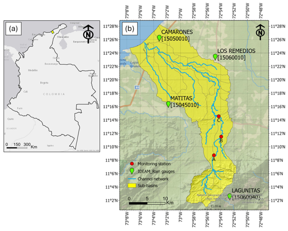
Figure 2.
Morphometric and geological characteristics of the watershed. (a) DEM-based (ALOS) topography and longitudinal profile of the main river channel. (b) Chronostratigraphic map showing the spatial distribution of the main geological units. Unit details are provided in the summarized geological table (Source: Atlas Geologico Colombiano at https://www.colombiaenmapas.gov.co).
Figure 2.
Morphometric and geological characteristics of the watershed. (a) DEM-based (ALOS) topography and longitudinal profile of the main river channel. (b) Chronostratigraphic map showing the spatial distribution of the main geological units. Unit details are provided in the summarized geological table (Source: Atlas Geologico Colombiano at https://www.colombiaenmapas.gov.co).
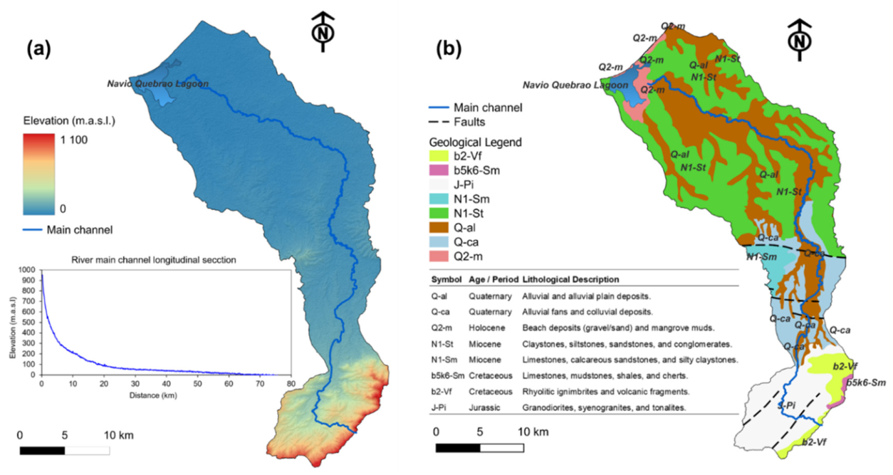
Figure 3.
Two emblematic faces of the Tomarrazón-Camarones basin: left) instream, manual but widespread sediment mining; right) the flora&fauna sanctuary Los Flamencos (Camarones coastal lagoon).
Figure 3.
Two emblematic faces of the Tomarrazón-Camarones basin: left) instream, manual but widespread sediment mining; right) the flora&fauna sanctuary Los Flamencos (Camarones coastal lagoon).
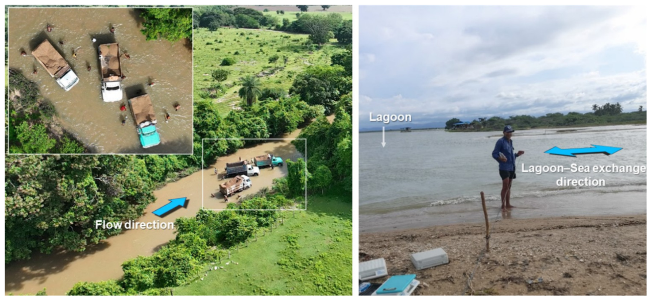
Figure 4.
The methodology adopted.
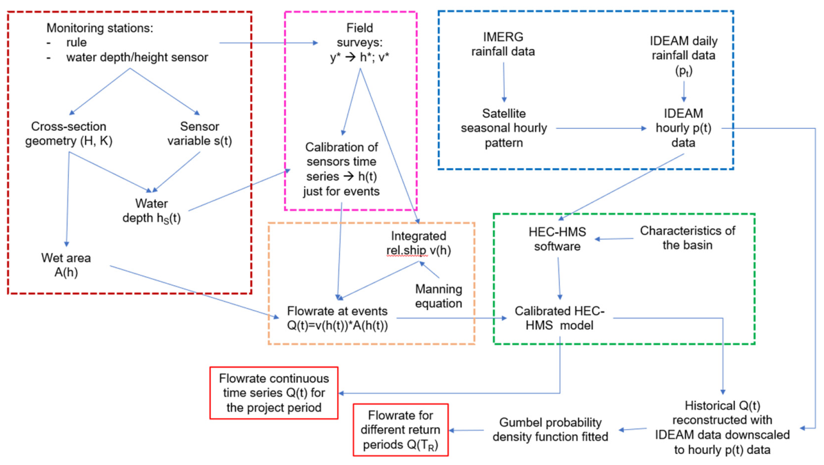
Figure 5.
Station B -Nueva Vida (as way of example): left) looking downstream; middle) the hydrometer during a slightly higher flowrate than normal, but yet not reaching the sensor; right) the Sonlist sensor installed (detail: 42 cm is the distance between the hanging hook and the zero of the rule).
Figure 5.
Station B -Nueva Vida (as way of example): left) looking downstream; middle) the hydrometer during a slightly higher flowrate than normal, but yet not reaching the sensor; right) the Sonlist sensor installed (detail: 42 cm is the distance between the hanging hook and the zero of the rule).
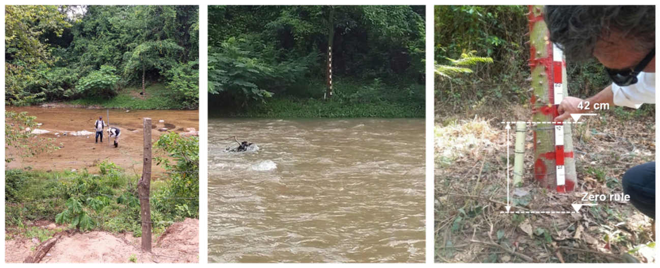
Figure 6.
A typical geometric cross section (Station A -Nueva Vida). All parameters are mentioned in the paragraph below.
Figure 6.
A typical geometric cross section (Station A -Nueva Vida). All parameters are mentioned in the paragraph below.
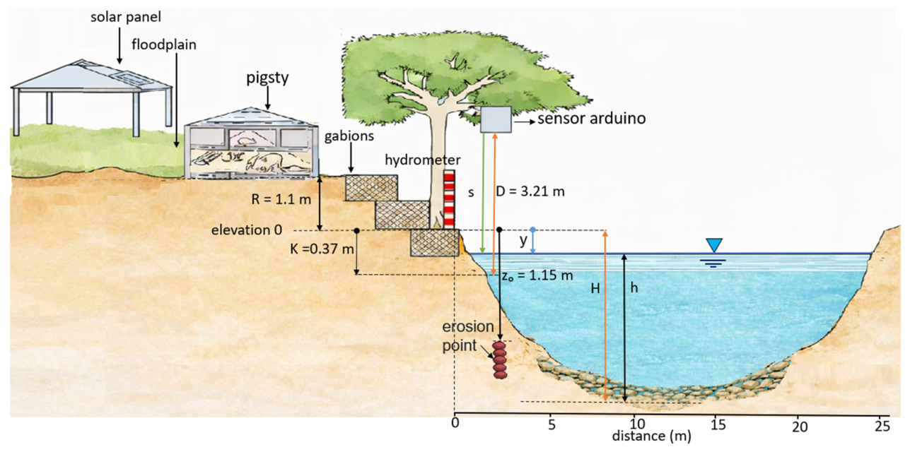
Figure 7.
Translating relevant variables into analogous ones at the Sonlist sensor cross section in the case of current flowing from the hydrometer towards the sensor cross section: (a) hydrometer section; (b) sensor section (some decameter downstream). Symbols defined below. Notice that in this case the zero of the hydrometer is particularly high (top) and hence y, y” are negative. More information regarding the parameters can be found in the section below.
Figure 7.
Translating relevant variables into analogous ones at the Sonlist sensor cross section in the case of current flowing from the hydrometer towards the sensor cross section: (a) hydrometer section; (b) sensor section (some decameter downstream). Symbols defined below. Notice that in this case the zero of the hydrometer is particularly high (top) and hence y, y” are negative. More information regarding the parameters can be found in the section below.
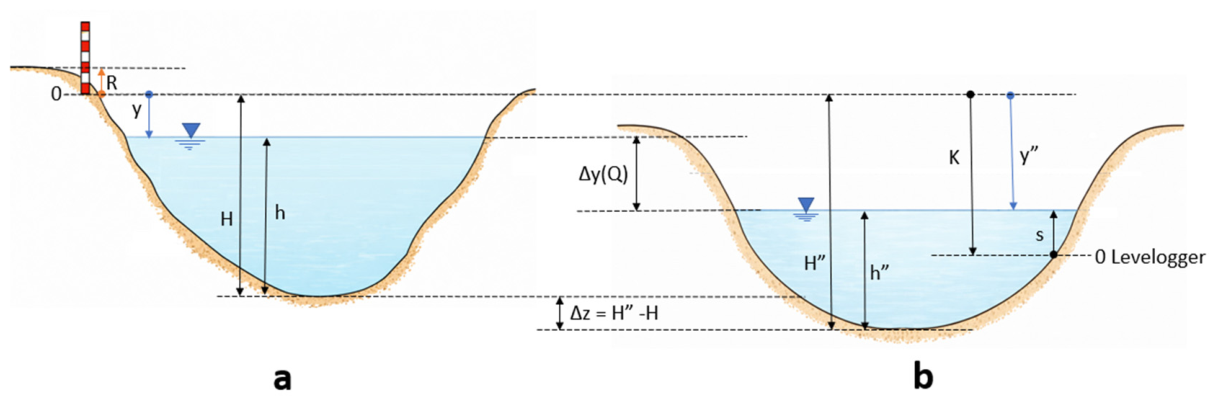
Figure 8.
Example of “calibration” of the water depth time series hs”(t) in station B geometrically derived from the sensor time series s(t) for the June 2025 events, into the corrected series h”(t) by time shift (the blue point belongs to the upstream station A and its blue curve does not fully capture it because it tradeoff has been searched among the different measures to be matched; it falls exactly on the red curve just by chance). Med A stands for discharge measurement.
Figure 8.
Example of “calibration” of the water depth time series hs”(t) in station B geometrically derived from the sensor time series s(t) for the June 2025 events, into the corrected series h”(t) by time shift (the blue point belongs to the upstream station A and its blue curve does not fully capture it because it tradeoff has been searched among the different measures to be matched; it falls exactly on the red curve just by chance). Med A stands for discharge measurement.
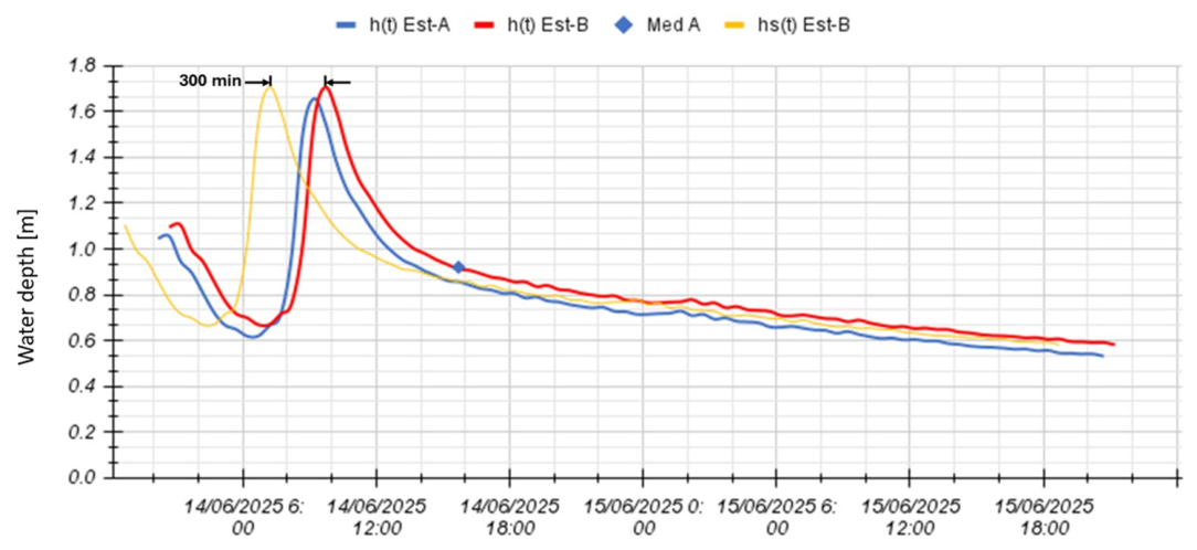
Figure 9.
Example of A(h) and v(h) functional relationships in station A.
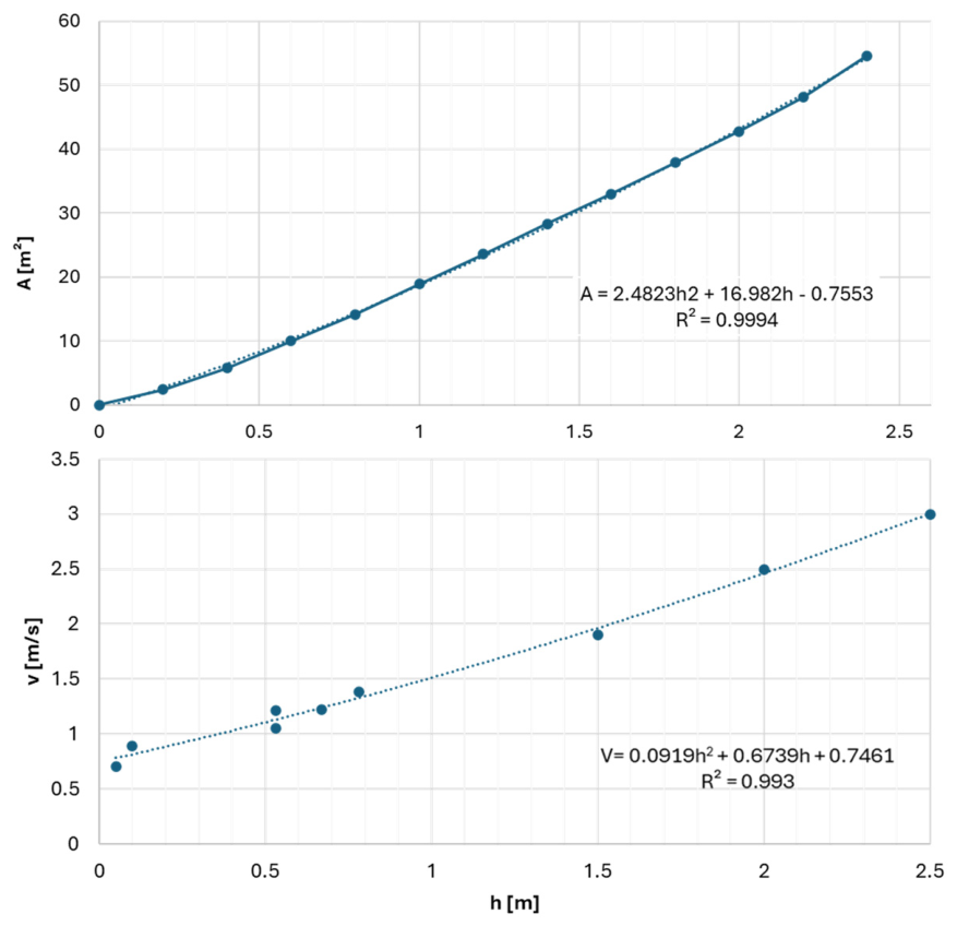
Figure 10.
Hourly distribution of precipitation in the Tomarrazón basin. (a) Daily distribution of precipitation, averaged over the whole IMERG data set available, in four discrete time portions for each month: morning (06-12h), afternoon (12-18h), evening (18-24h) and night (00-06h). As an example, considering November, the most intense rainy period, it is apparent that only a small fraction of the total precipitation occurs in daily hours (morning and afternoon); (b) Example of the hourly precipitation pattern in a average day of November.
Figure 10.
Hourly distribution of precipitation in the Tomarrazón basin. (a) Daily distribution of precipitation, averaged over the whole IMERG data set available, in four discrete time portions for each month: morning (06-12h), afternoon (12-18h), evening (18-24h) and night (00-06h). As an example, considering November, the most intense rainy period, it is apparent that only a small fraction of the total precipitation occurs in daily hours (morning and afternoon); (b) Example of the hourly precipitation pattern in a average day of November.
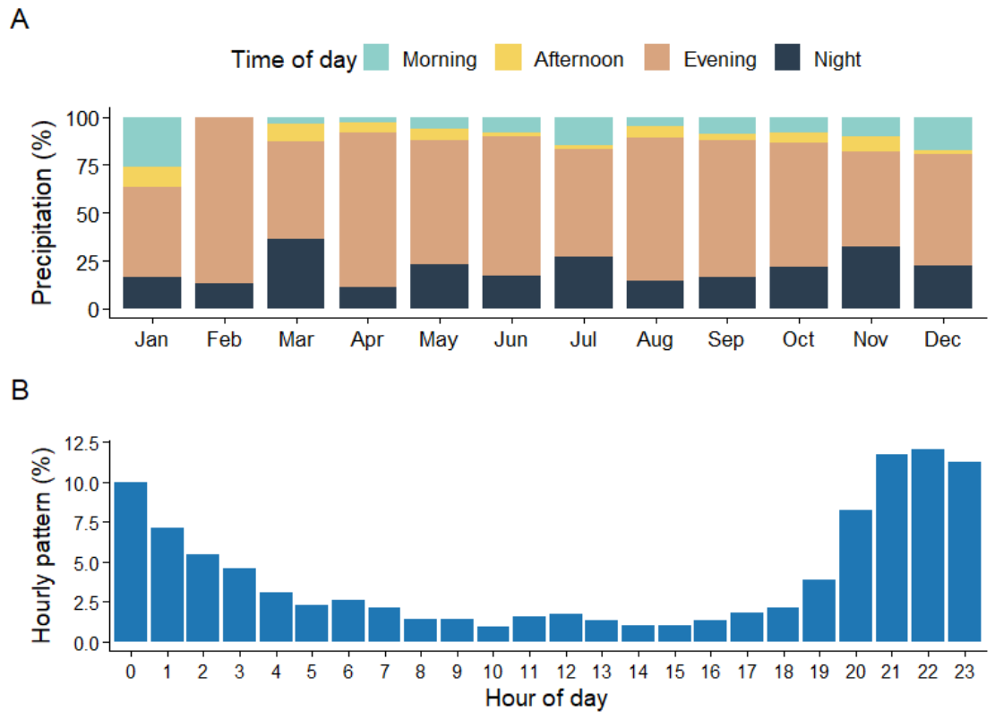
Figure 11.
Hydrograph recorded in the three stations A, B, C (from top to bottom), light blue, and flow rate time series Q(t) reconstructed by the calibrated model (black line). The grey areas identify time Interval where there are no sensors measurements (too low flows or device anomalies). Stations A, B were used in calibration while C in validation.
Figure 11.
Hydrograph recorded in the three stations A, B, C (from top to bottom), light blue, and flow rate time series Q(t) reconstructed by the calibrated model (black line). The grey areas identify time Interval where there are no sensors measurements (too low flows or device anomalies). Stations A, B were used in calibration while C in validation.
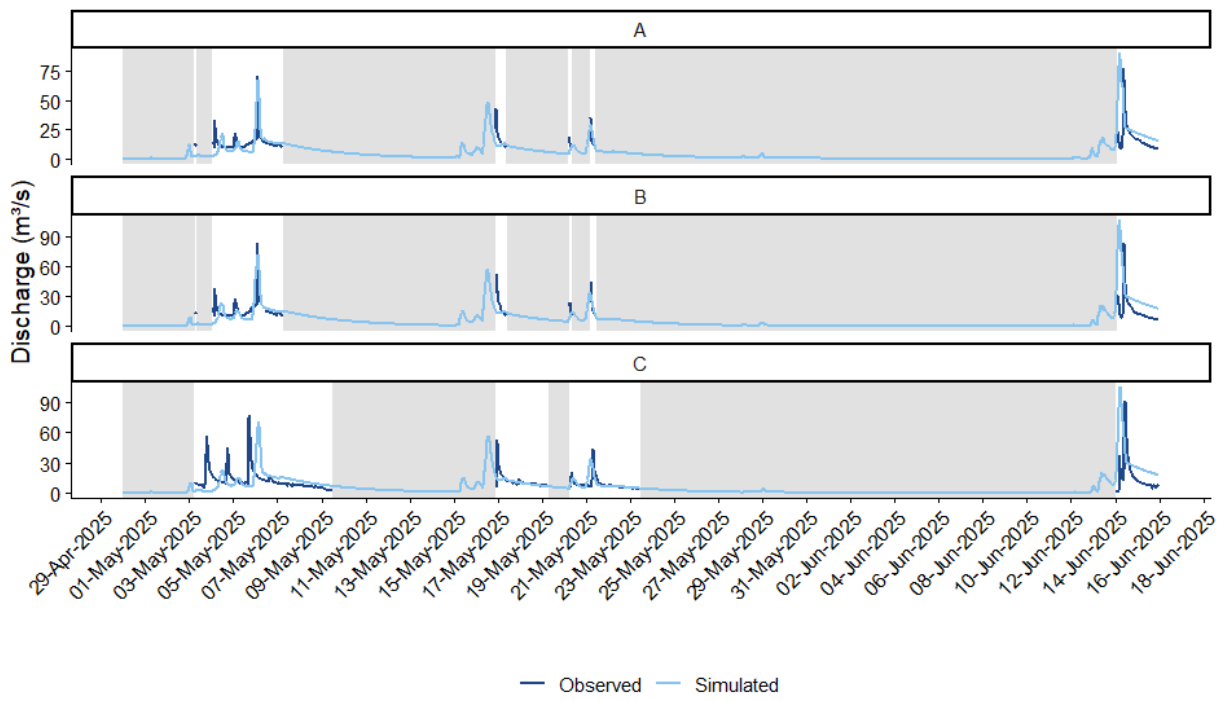
Figure 12.
Calibration: left) performance of different attempts in the two criteria plan (the Pareto frontier is identified) and the parametrization eventually selected. The grey area represents a break in the y-axis, from 0.2 to 0.9. Right) the indicative overall performance (square root of quadratic normalized indices) of the attempts explored. NOTE that the preferred parametrization is not, in principle, the one that minimizes the overall index square root of the sum of the two indices adopted: that is just an indicative choice of a particular multi-objective choice criterion that implies having given a certain relative preference to the indices. It is shown in the figure just for ease of representation.
Figure 12.
Calibration: left) performance of different attempts in the two criteria plan (the Pareto frontier is identified) and the parametrization eventually selected. The grey area represents a break in the y-axis, from 0.2 to 0.9. Right) the indicative overall performance (square root of quadratic normalized indices) of the attempts explored. NOTE that the preferred parametrization is not, in principle, the one that minimizes the overall index square root of the sum of the two indices adopted: that is just an indicative choice of a particular multi-objective choice criterion that implies having given a certain relative preference to the indices. It is shown in the figure just for ease of representation.
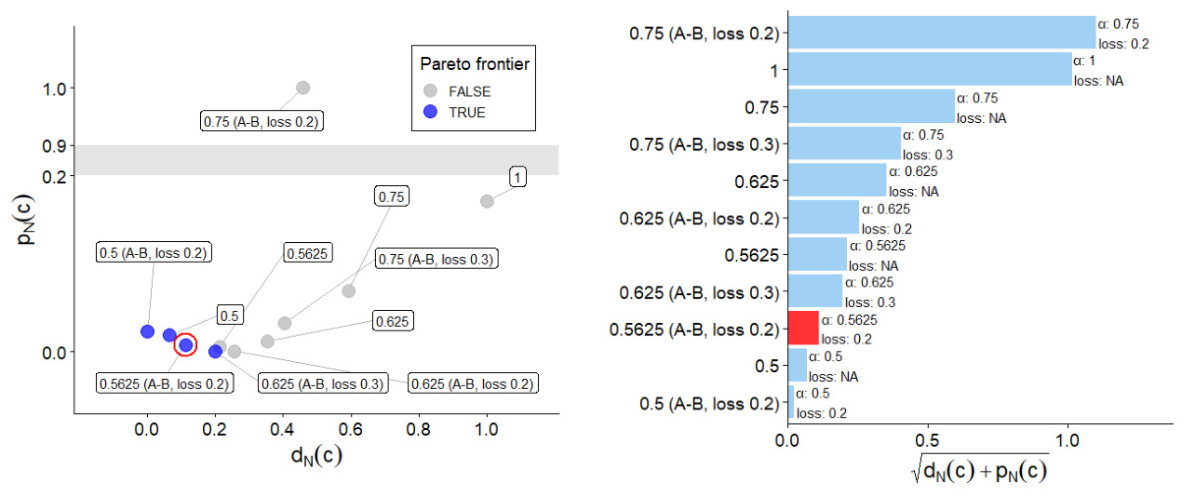
Figure 13.
Performance in calibration (duration curves at station A+B on the left) and validation (duration curves at station C, in the middle, and peaks deviation on the right). Notice that the duration curves are not reliable for low flows (about Q<10 m3/s because the sensors do not detect them).
Figure 13.
Performance in calibration (duration curves at station A+B on the left) and validation (duration curves at station C, in the middle, and peaks deviation on the right). Notice that the duration curves are not reliable for low flows (about Q<10 m3/s because the sensors do not detect them).
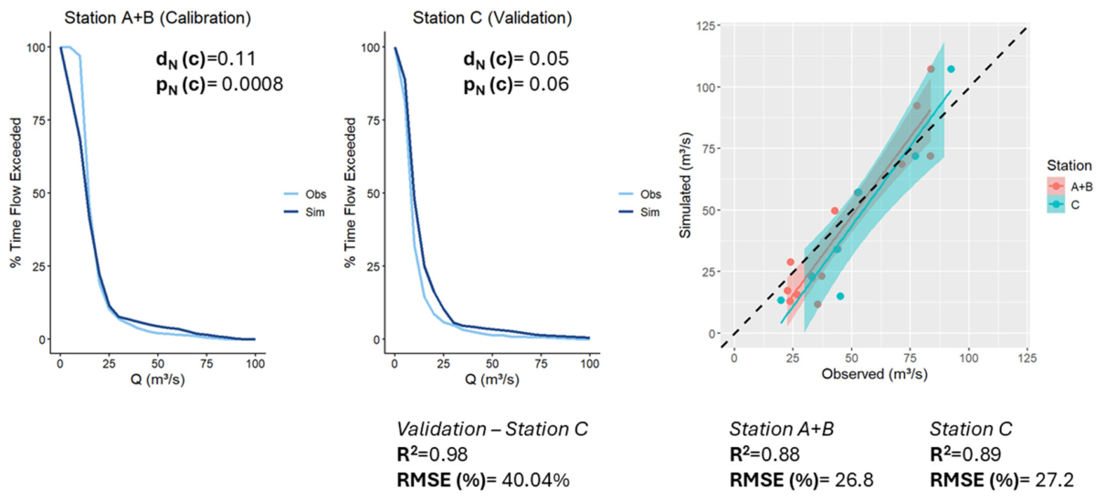
Figure 14.
Historical hydrology: A) fitted probability distribution and corresponding return periods of characteristic magnitude; B) reconstructed flowrate QH(t) time pattern.
Figure 14.
Historical hydrology: A) fitted probability distribution and corresponding return periods of characteristic magnitude; B) reconstructed flowrate QH(t) time pattern.
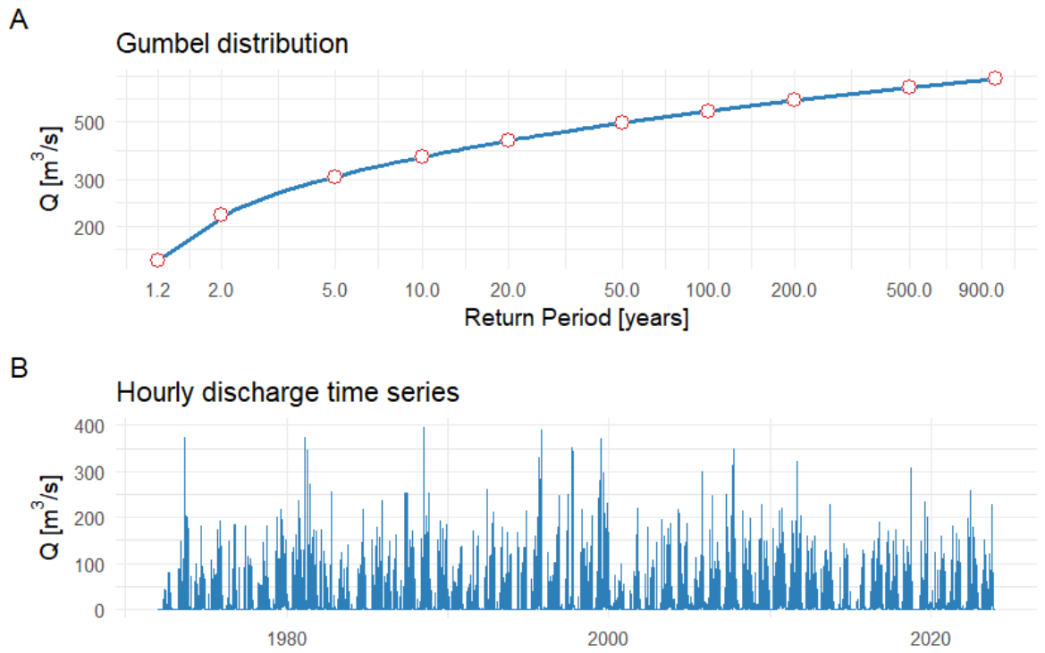

Table 1.
Satellite data used to identify the hourly time pattern of precipitation inside the basin of interest.
Table 1.
Satellite data used to identify the hourly time pattern of precipitation inside the basin of interest.
| Product name | Spatial resolution | Temporal | Period |
Free access |
access platform |
Required Processing |
|
IMERG |
0.1° × 0.1° (~10 km) | 30 min | Jan 2014 -Dec 2023 | Yes | GE® | Basin-scale spatial extraction and aggregation (spatialization) |
Disclaimer/Publisher’s Note: The statements, opinions and data contained in all publications are solely those of the individual author(s) and contributor(s) and not of MDPI and/or the editor(s). MDPI and/or the editor(s) disclaim responsibility for any injury to people or property resulting from any ideas, methods, instructions or products referred to in the content. |
© 2026 by the authors. Licensee MDPI, Basel, Switzerland. This article is an open access article distributed under the terms and conditions of the Creative Commons Attribution (CC BY) license (http://creativecommons.org/licenses/by/4.0/).
Copyright: This open access article is published under a Creative Commons CC BY 4.0 license, which permit the free download, distribution, and reuse, provided that the author and preprint are cited in any reuse.


