A Comparative Study of Machine Learning Algorithms for Type 2 Diabetes Stage Classification Using Clinical and Lifestyle Features

1. Introduction

Type 2 diabetes mellitus (T2DM) has emerged as one of the most critical non-communicable disease crises of the twenty-first century. The 11th edition of the International Diabetes Federation (IDF) Diabetes Atlas reports that 589 million adults aged 20-79 years were living with diabetes in 2024 - representing one in nine of the global adult population - with projections indicating a rise to 853 million by 2050 [1]. The disease caused an estimated 3.4 million deaths and generated USD 1.015 trillion in global health expenditure in the same year [1]. In Southeast Asia, Indonesia bears a disproportionate burden, ranking fourth globally with over 19.5 million cases recorded in 2021 [2], making it an unavoidable public health priority.

Effective management of T2DM is fundamentally dependent on accurate clinical staging at the earliest possible point. The American Diabetes Association (ADA) defines pre-diabetes as a fasting plasma glucose level of 100-125 mg/dL or HbA1c of 5.7-6.4%, and confirmed T2DM at fasting plasma glucose >= 126 mg/dL or HbA1c >= 6.5% [3]. Stratification into these three clinical classes carries high therapeutic significance: targeted lifestyle interventions at the pre-diabetic stage have been demonstrated to prevent or delay progression to overt T2DM [4,5]. Yet conventional screening continues to rely on laboratory investigations interpreted by specialists - a model fundamentally ill-suited to resource-constrained primary healthcare settings, precisely where the diabetes burden is growing most rapidly.

Machine learning (ML) offers a compelling and scalable route to automated population-level staging, through its capacity to identify complex, non-linear patterns in heterogeneous clinical and behavioural data. A growing body of literature has explored ML-based diabetes classification, producing valuable but methodologically varied findings. Iparraguirre-Villanueva et al. [7] applied seven classical classifiers to an augmented version of the Pima Indians dataset and reported Decision Tree as the best binary classifier at 80.2% accuracy, while k-NN performance was sensitive to neighbourhood size with optimal results at k=5. Al Sadi and Balachandran [8] compared seven ML algorithms on an Omani pre-diabetic cohort of 502 patients and found that Random Forest and k-NN (k=5) achieved the best performance, though evaluation was restricted to a single 70/30 split. Chen et al. [9] applied six models to a large Chinese clinical cohort, with a backpropagation neural network achieving 93.7% accuracy and AUC = 0.977, corroborating the primacy of glycaemic biomarkers as predictors. Ordóñez-Guillén et al. [10] addressed T2DM subtype classification using ML on combined NHANES and ENSANUT datasets (N = 10,077), achieving 88.3% accuracy via 5-fold cross-validation. Rashid et al. [11] proposed a CNN-BiLSTM deep learning architecture achieving 96.7% accuracy on a binary task, though at the cost of interpretability and computational overhead. Most directly comparable to the present work, Datta et al. [12] applied supervised ensemble voting to multi-class diabetes staging and reported 90.1% accuracy, yet relied on a single-institution dataset without systematic cross-algorithm comparison.

Collectively, these studies reveal three persistent methodological gaps: (i) the majority of investigations frame diabetes classification as a binary problem, obscuring the pre-diabetes stage as a clinically distinct class [6,7]; (ii) performance estimates are frequently derived from a single validation split, rendering them susceptible to selection bias [8]; and (iii) cross-algorithm benchmarking under multiple validation paradigms on large-scale, multinational datasets remains scarce [9,10]. This study is designed to address all three gaps through three principal contributions. First, diabetes classification is explicitly formulated as a three-class problem - Normal, Pre-diabetes, and Diabetes - in alignment with the WHO/ADA clinical taxonomy. Second, four classification algorithms - k-NN (five configurations of k), Decision Tree (DT), Gaussian Naive Bayes (NB), and Multi-Layer Perceptron Neural Network (MLP-NN) - are rigorously benchmarked under four validation strategies (5-fold CV, 10-fold CV, 80/20 hold-out, and 90/10 hold-out) to produce robust and reproducible performance estimates. Third, the most discriminative clinical predictors are identified to provide actionable insight for the design of ML-based clinical decision support systems.

2. Methods

2.1. Research Design and Methodology Overview

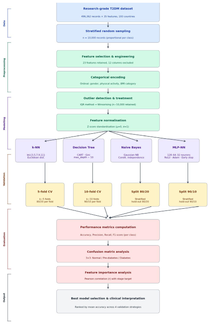
The overall research methodology is structured as a six-phase sequential pipeline. The phases comprise: (1) data acquisition and stratified sampling, (2) feature selection and engineering, (3) pre-processing, (4) model training across four classification algorithms and five k-NN configurations, (5) multi-strategy validation, and (6) performance evaluation and model selection.

2.2. Dataset

The Type 2 Diabetes Risk Dataset v3, publicly available on Kaggle [26], was employed in this study. Curated by Mubashar Ahmed Rabbani, the dataset aggregates longitudinal clinical records from 193 countries spanning the period 1976-2026, yielding 496,362 patient observations across 35 variables. The target variable 'stage' encodes three mutually exclusive classes: Normal (stage 0), Pre-diabetes (stage 2), and Diabetes (stage 3), aligned with ADA (2023) clinical taxonomy. A stratified random sample of 10,000 records yielded a class distribution of 2,776 Normal (27.8%), 2,871 Pre-diabetes (28.7%), and 4,353 Diabetes (43.5%) instances. No class falls below 10%, supporting the use of overall accuracy as a primary performance metric.

Figure 1. End-to-end research methodology flowchart. Phases are colour-coded: blue (data), teal (pre-processing), purple (modelling), amber (validation), red (evaluation), and gray (output).

Figure 1. End-to-end research methodology flowchart. Phases are colour-coded: blue (data), teal (pre-processing), purple (modelling), amber (validation), red (evaluation), and gray (output).

2.3. Pre-Processing Pipeline

2.3.1. Feature Selection

Twelve columns were excluded prior to analysis: patient identifier, observation year, onset year, binary diabetes onset indicator, five-year diabetes risk projection, composite risk score, prior-year glucose, prior-year BMI, survival indicator, and country code. The retained 23-feature set spans five clinical domains: anthropometric indices, glycaemic biomarkers, metabolic/endocrine markers, lipid profile, and lifestyle/psychosocial factors.

2.3.2. Categorical Encoding

Three object-type variables were converted to ordinal integer representations: (i) gender: Female = 0, Male = 1; (ii) physical_activity: low = 0, medium = 1, high = 2; (iii) BMI_category: Underweight = 0, Normal = 1, Overweight = 2, Obese = 3, aligned with WHO body weight classification.

2.3.3. Outlier Detection and Treatment

Outlier detection was performed using the Interquartile Range (IQR) method on 12 continuous features. For each feature x, outlier boundaries were defined as:

Lower bound = Q1 - 1.5 x IQR

(1)

Upper bound = Q3 + 1.5 x IQR, where IQR = Q3 - Q1

(2)

Values exceeding these bounds were treated via Winsorising. The fasting plasma glucose variable exhibited the highest outlier count (n = 127; upper bound = 204.3 mg/dL).

2.3.4. Feature Normalisation

All 23 features were standardised using Z-score normalisation prior to model training. For each feature x, the transformation is:

x’ = (x - mu) / sigma

(3)

where mu is the feature mean and sigma is the standard deviation computed on the training set.

2.4. Classification Algorithms

2.4.1. k-Nearest Neighbour (k-NN)

The k-NN algorithm classifies an unseen instance x_q by majority vote over its k nearest neighbours in the training set [13]. Five values of k were evaluated: k in {3, 5, 7, 9, 11}. All values are odd to eliminate tie-breaking ambiguity.

y_hat = argmax_{c in C} |{x_i in N_k(x_q) : y_i = c}|

(4)

$$d(x\_q,x\_i)=sqrt(sum\_\{j1\}^\{p\left\}\right(x\_\{q,j\}-x\_\{i,j\})^2)$$

(5)

2.4.2. Decision Tree (CART)

The CART algorithm [14] recursively partitions the feature space by selecting the split that maximises the reduction in Gini impurity:

Gini(t) = 1 - sum_{c in C} p(c|t)^2

(6)

DeltaGini = Gini(t) - (n_L/n_t)*Gini(t_L) - (n_R/n_t)*Gini(t_R)

(7)

A maximum depth of 10 was imposed to mitigate overfitting.

2.4.3. Gaussian Naive Bayes (NB)

The Gaussian NB classifier [15] applies Bayes' theorem under the assumption of conditional feature independence:

y_hat = argmax_{c} P(c) * prod_{j} P(x_j|c)

(8)

P(x_j|c) = (1/sqrt(2*pi*sigma_{jc}^2)) * exp(-(x_j-mu_{jc})^2 / (2*sigma_{jc}^2))

(9)

2.4.4. Multi-Layer Perceptron Neural Network (MLP-NN)

The MLP-NN [16] is a feedforward neural network with three fully connected hidden layers of 128, 64, and 32 neurons respectively. The output of hidden layer l is:

h^(l) = f( W^(l) * h^(l-1) + b^(l) )

(10)

f(z) = max(0, z)

(11)

P(y=c|x) = exp(z_c) / sum_{k} exp(z_k)

(12)

L = -sum_i sum_c y_{ic} * log P(y_i=c|x_i)

(13)

The network is trained using the Adam optimiser [17] with default hyperparameters. A maximum of 1,000 training epochs was specified with early stopping (patience=10, validation fraction=10%).

2.5. Validation Strategy

Four complementary validation strategies were employed: (i) stratified 5-fold CV, (ii) stratified 10-fold CV, (iii) hold-out 80%/20%, and (iv) hold-out 90%/10% with random state 42. Estimated cross-validation accuracy:

ACC_CV = (1/k) * sum_{i=1}^{k} ACC_i

(14)

2.6. Evaluation Metrics

Model performance was assessed using overall accuracy, per-class precision, recall, and F1-score:

ACC = (TP + TN) / (TP + TN + FP + FN)

(15)

Precision_c = TP_c / (TP_c + FP_c)

(16)

Recall_c = TP_c / (TP_c + FN_c)

(17)

F1_c = 2*(Precision_c * Recall_c) / (Precision_c + Recall_c)

(18)

3. Results and Discussions

3.1. Descriptive Statistics

Table 1 summarises descriptive statistics for 12 principal continuous features of the 10,000-record analytical sample. The mean fasting plasma glucose of 111.86 mg/dL (SD = 38.07) places the sample in the ADA pre-diabetic range. Mean HOMA-IR of 4.35 substantially exceeds the normal threshold of 2.5, indicating pervasive insulin resistance.

3.2. Feature Correlation Analysis

Table 2 presents Pearson correlation coefficients between continuous features and the target variable, providing empirical support for the feature set.

3.3. Classification Performance

Table 3 presents classification accuracy (%) for all model configurations across the four validation strategies. The MLP-NN achieved the highest mean accuracy of 91.38%, closely followed by the Decision Tree at 91.10%.

3.4. Per-Class Performance of the Best Model

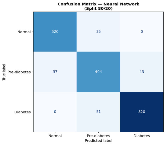
Table 4 reports per-class precision, recall, and F1-score for the MLP-NN on the 80/20 hold-out split. The Diabetes class achieved the highest F1-score (0.946), while Pre-diabetes showed the lowest (0.856).

3.5. Effect of Neighbourhood Size on k-NN

A monotonically increasing relationship was observed between k and classification accuracy. Accuracy improved from 83.73% (k=3) to 87.09% (k=11), a 3.36 percentage-point gain. The improvement rate decelerated with increasing k, suggesting approach to a local optimum within the tested range.

Figure 2. Effect of neighbourhood size k on k-NN accuracy across four validation strategies.

Figure 2. Effect of neighbourhood size k on k-NN accuracy across four validation strategies.

Figure 3. Comparative accuracy for all model configurations under four validation strategies.

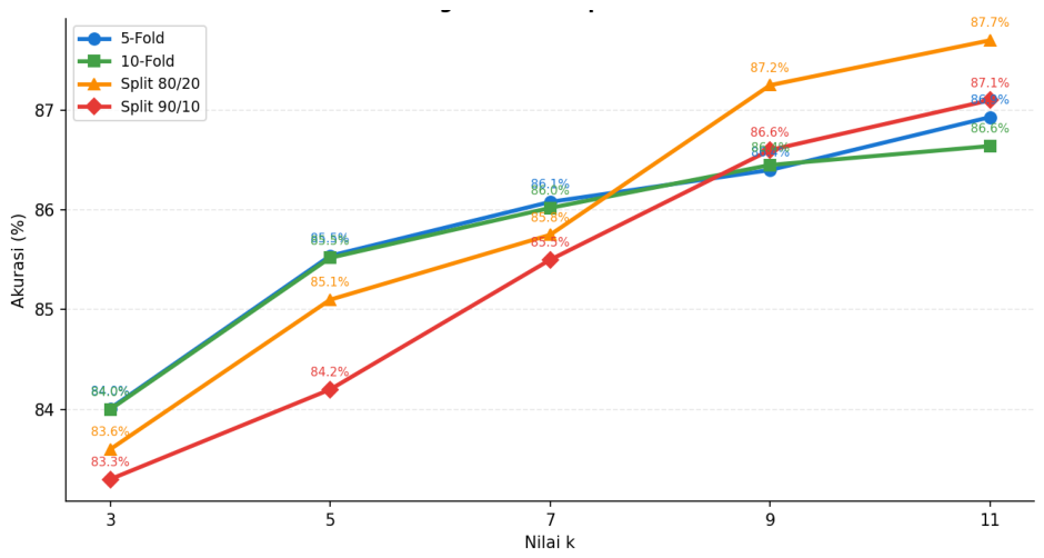
Figure 3. Comparative accuracy for all model configurations under four validation strategies.

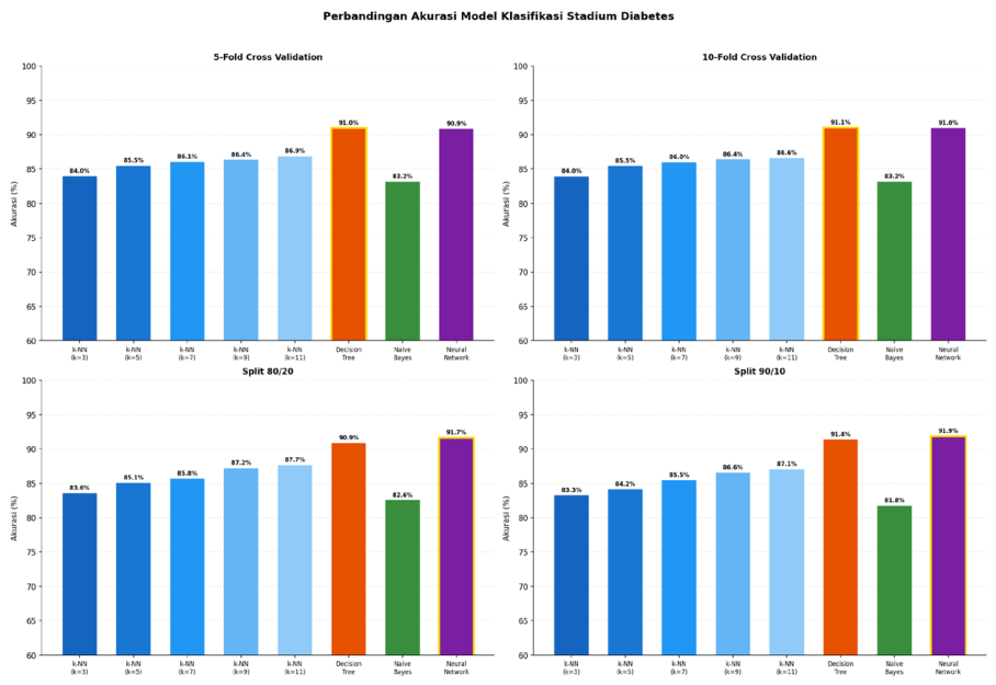
Figure 4. Confusion matrix for MLP-NN on 80/20 hold-out split (n = 2,000).

Figure 4. Confusion matrix for MLP-NN on 80/20 hold-out split (n = 2,000).

3.6. Statistical Significance Testing

To validate that observed performance differences are not attributable to sampling variability, four complementary statistical analyses were conducted: Friedman test, Wilcoxon signed-rank post-hoc test with Holm-Bonferroni correction, Cohen's kappa coefficient, and McNemar's test [18,19].

3.6.1. Friedman Test (Global Comparison)

The Friedman test is a non-parametric test comparing k classifiers across n independent evaluation folds without normality assumptions [18]:

FF = [(12n)/(k(k+1))] * [sum_j Rj^2 - k(k+1)^2/4] / [1 - SSe/SSt]

(19)

Table 5. Friedman test results: mean accuracy, standard deviation, and average rank per classifier across 10 folds.

Model	Mean Acc. (%)	SD (%)	Avg. Rank	Rank
Neural Network	90.93	0.74	1.200	1st
Decision Tree	90.93	0.72	1.800	2nd
k-NN (k=11)	86.82	0.89	3.700	3rd
k-NN (k=9)	86.51	0.70	4.000	4th
k-NN (k=7)	86.12	0.98	4.600	5th
k-NN (k=5)	85.52	0.73	5.700	6th
k-NN (k=3)	83.69	0.79	7.400	7th
Naive Bayes	83.15	0.93	7.600	8th

Table 5. Friedman test results: mean accuracy, standard deviation, and average rank per classifier across 10 folds.

Model	Mean Acc. (%)	SD (%)	Avg. Rank	Rank
Neural Network	90.93	0.74	1.200	1st
Decision Tree	90.93	0.72	1.800	2nd
k-NN (k=11)	86.82	0.89	3.700	3rd
k-NN (k=9)	86.51	0.70	4.000	4th
k-NN (k=7)	86.12	0.98	4.600	5th
k-NN (k=5)	85.52	0.73	5.700	6th
k-NN (k=3)	83.69	0.79	7.400	7th
Naive Bayes	83.15	0.93	7.600	8th

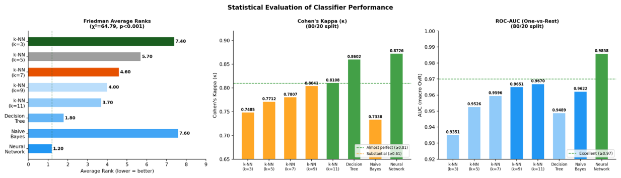
The Friedman test yielded chi-squared(7) = 64.79, p < 0.001, providing overwhelming evidence to reject H0. Neural Network ranked best (1.200), Naive Bayes worst (7.600).

3.6.2. Wilcoxon Signed-Rank Post-hoc Test

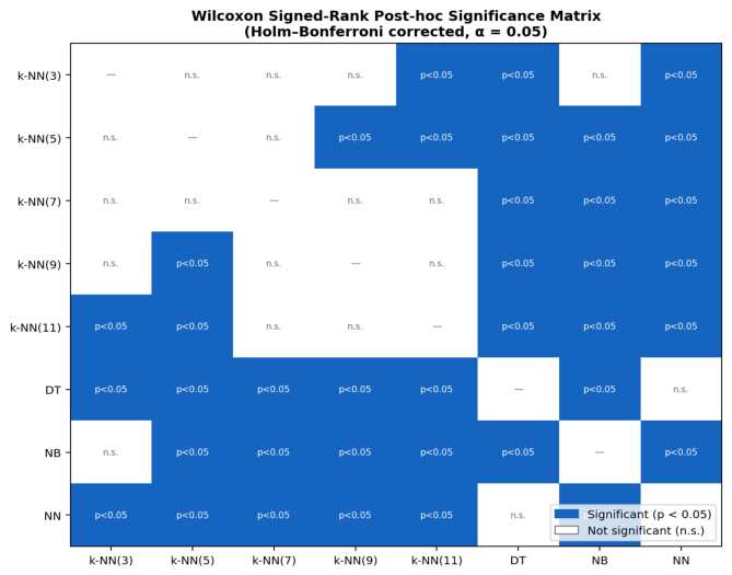
Pairwise Wilcoxon signed-rank tests were applied to all 28 model pairs across 10 per-fold accuracy vectors. Holm-Bonferroni correction was applied. Key findings: Neural Network and Decision Tree are statistically indistinguishable (adj. p = 0.762); both are significantly superior to all k-NN configurations and Naive Bayes.

Figure 5. Wilcoxon post-hoc significance matrix (Holm-Bonferroni, alpha = 0.05). Blue = significant (p < 0.05); white = n.s.

Figure 5. Wilcoxon post-hoc significance matrix (Holm-Bonferroni, alpha = 0.05). Blue = significant (p < 0.05); white = n.s.

3.6.3. Cohen's Kappa Coefficient

Cohen's kappa quantifies classifier agreement beyond chance:

kappa = (P_o - P_e) / (1 - P_e)

(20)

Table 6. Cohen's kappa (kappa) for all classifiers on 80/20 hold-out split.

Model	Accuracy (%)	Cohen's kappa	Interpretation
Neural Network	91.70	0.8726	Almost perfect
Decision Tree	90.90	0.8602	Almost perfect
k-NN (k=11)	87.70	0.8108	Almost perfect
k-NN (k=9)	87.25	0.8041	Almost perfect
k-NN (k=7)	85.75	0.7807	Substantial
k-NN (k=5)	85.10	0.7712	Substantial
k-NN (k=3)	83.60	0.7485	Substantial
Naive Bayes	82.60	0.7338	Substantial

Table 6. Cohen's kappa (kappa) for all classifiers on 80/20 hold-out split.

Model	Accuracy (%)	Cohen's kappa	Interpretation
Neural Network	91.70	0.8726	Almost perfect
Decision Tree	90.90	0.8602	Almost perfect
k-NN (k=11)	87.70	0.8108	Almost perfect
k-NN (k=9)	87.25	0.8041	Almost perfect
k-NN (k=7)	85.75	0.7807	Substantial
k-NN (k=5)	85.10	0.7712	Substantial
k-NN (k=3)	83.60	0.7485	Substantial
Naive Bayes	82.60	0.7338	Substantial

3.6.4. McNemar's Test

McNemar's test evaluates whether two classifiers make statistically different error patterns on the same test set. The continuity-corrected statistic is:

chi2 = (|b - c| - 1)^2 / (b + c)

(21)

Table 7. McNemar's test: Neural Network vs all other classifiers (80/20 split).

Comparison	chi-squared	p-value	Decision
NN vs k-NN (k=3)	93.917	< 0.001***	NN significantly better
NN vs k-NN (k=5)	69.198	< 0.001***	NN significantly better
NN vs k-NN (k=7)	59.760	< 0.001***	NN significantly better
NN vs k-NN (k=9)	36.701	< 0.001***	NN significantly better
NN vs k-NN (k=11)	32.170	< 0.001***	NN significantly better
NN vs Decision Tree	1.264	0.261 (n.s.)	No significant difference
NN vs Naive Bayes	108.480	< 0.001***	NN significantly better

Neural Network is significantly superior to all k-NN configurations and Naive Bayes (p < 0.001), but not to the Decision Tree (p = 0.261). This confirms that Neural Network and Decision Tree are statistically equivalent despite the 0.80% accuracy gap.

Table 7. McNemar's test: Neural Network vs all other classifiers (80/20 split).

Comparison	chi-squared	p-value	Decision
NN vs k-NN (k=3)	93.917	< 0.001***	NN significantly better
NN vs k-NN (k=5)	69.198	< 0.001***	NN significantly better
NN vs k-NN (k=7)	59.760	< 0.001***	NN significantly better
NN vs k-NN (k=9)	36.701	< 0.001***	NN significantly better
NN vs k-NN (k=11)	32.170	< 0.001***	NN significantly better
NN vs Decision Tree	1.264	0.261 (n.s.)	No significant difference
NN vs Naive Bayes	108.480	< 0.001***	NN significantly better

Neural Network is significantly superior to all k-NN configurations and Naive Bayes (p < 0.001), but not to the Decision Tree (p = 0.261). This confirms that Neural Network and Decision Tree are statistically equivalent despite the 0.80% accuracy gap.

3.6.5. ROC-AUC Analysis

Macro-averaged One-vs-Rest ROC-AUC was computed for the three-class problem:

Table 8. Macro-averaged ROC-AUC (OvR) for all classifiers on 80/20 hold-out split.

Model	AUC (OvR macro)	Interpretation
Neural Network	0.9858	Outstanding
k-NN (k=11)	0.9670	Excellent
k-NN (k=9)	0.9651	Excellent
Naive Bayes	0.9622	Excellent
k-NN (k=7)	0.9596	Excellent
k-NN (k=5)	0.9526	Excellent
Decision Tree	0.9489	Excellent
k-NN (k=3)	0.9351	Excellent

Table 8. Macro-averaged ROC-AUC (OvR) for all classifiers on 80/20 hold-out split.

Model	AUC (OvR macro)	Interpretation
Neural Network	0.9858	Outstanding
k-NN (k=11)	0.9670	Excellent
k-NN (k=9)	0.9651	Excellent
Naive Bayes	0.9622	Excellent
k-NN (k=7)	0.9596	Excellent
k-NN (k=5)	0.9526	Excellent
Decision Tree	0.9489	Excellent
k-NN (k=3)	0.9351	Excellent

Figure 6. Statistical metrics: (A) Friedman average ranks, (B) Cohen's kappa with interpretive thresholds, (C) Macro-averaged ROC-AUC.

Figure 6. Statistical metrics: (A) Friedman average ranks, (B) Cohen's kappa with interpretive thresholds, (C) Macro-averaged ROC-AUC.

3.6.6. Consolidated Statistical Summary

Table 9. Consolidated statistical summary: all four tests across all classifiers.

Model	Avg. Rank	kappa	AUC	McNemar vs NN	Verdict
Neural Network	1.200	0.8726	0.9858	—	Best / top cluster
Decision Tree	1.800	0.8602	0.9489	n.s.	Equiv. to NN
k-NN (k=11)	3.700	0.8108	0.9670	p<0.001	Below top-2
k-NN (k=9)	4.000	0.8041	0.9651	p<0.001	Below top-2
k-NN (k=7)	4.600	0.7807	0.9596	p<0.001	Below top-2
k-NN (k=5)	5.700	0.7712	0.9526	p<0.001	Below top-2
k-NN (k=3)	7.400	0.7485	0.9351	p<0.001	Below top-2
Naive Bayes	7.600	0.7338	0.9622	p<0.001	Below top-2

Converging evidence from all four tests confirms two statistically distinct performance clusters: (1) Neural Network and Decision Tree form a superior cluster, statistically equivalent to each other but significantly better than all other classifiers; (2) k-NN and Naive Bayes form a lower-performing cluster.

Table 9. Consolidated statistical summary: all four tests across all classifiers.

Model	Avg. Rank	kappa	AUC	McNemar vs NN	Verdict
Neural Network	1.200	0.8726	0.9858	—	Best / top cluster
Decision Tree	1.800	0.8602	0.9489	n.s.	Equiv. to NN
k-NN (k=11)	3.700	0.8108	0.9670	p<0.001	Below top-2
k-NN (k=9)	4.000	0.8041	0.9651	p<0.001	Below top-2
k-NN (k=7)	4.600	0.7807	0.9596	p<0.001	Below top-2
k-NN (k=5)	5.700	0.7712	0.9526	p<0.001	Below top-2
k-NN (k=3)	7.400	0.7485	0.9351	p<0.001	Below top-2
Naive Bayes	7.600	0.7338	0.9622	p<0.001	Below top-2

Converging evidence from all four tests confirms two statistically distinct performance clusters: (1) Neural Network and Decision Tree form a superior cluster, statistically equivalent to each other but significantly better than all other classifiers; (2) k-NN and Naive Bayes form a lower-performing cluster.

3.7. Discussion

The central finding of this study is that the MLP-NN achieved the highest mean accuracy (91.38%) for three-stage T2DM classification across all validation strategies, closely followed by the Decision Tree (91.10%). These results carry several important implications.

The marginal superiority of MLP-NN over the Decision Tree (0.28 percentage points) warrants careful interpretation. The MLP-NN demonstrated a positive trend across validation strategies, indicating that the model benefits from larger training sets. By contrast, the Decision Tree showed near-constant performance, suggesting it had reached its representational capacity at 80% training data with max_depth = 10. In contexts where model interpretability is paramount, the Decision Tree may be preferred given its ability to be expressed as explicit if-then rules that clinicians can directly audit.

The high accuracy of both models is primarily attributable to the strong discriminative power of glycaemic biomarkers. Fasting plasma glucose (r = 0.67) and HbA1c (r = 0.59) both correspond directly to WHO/ADA diagnostic thresholds, creating relatively well-separated class distributions. The MLP-NN captures the same boundaries and additionally models higher-order feature interactions between glycaemia, insulin resistance (HOMA-IR), and anthropometric variables.

The k-NN algorithm's monotonic improvement with increasing k reflects the bias-variance tradeoff for instance-based learners. The k=11 configuration (87.09%) remained well below the top two models, likely due to the curse of dimensionality in a 23-dimensional space [20]. Dimensionality reduction or distance-weighted variants may improve k-NN in this context.

Gaussian Naive Bayes yielded the lowest accuracy (82.70%), consistent with the known limitation of its conditional independence assumption in the presence of correlated clinical biomarkers. The declining accuracy from cross-validation (83.20%) to the 90/10 split (81.80%) indicates further sensitivity to training set size.

The lower F1-score for the Pre-diabetes class (0.856 vs. 0.935-0.946 for Normal and Diabetes) merits clinical attention. Pre-diabetes represents the highest-priority intervention stage because lifestyle modification at this point has demonstrated efficacy in preventing T2DM onset [4,5]. Cost-sensitive learning approaches represent a promising direction for future work.

Several limitations should be acknowledged. First, the dataset was synthetically augmented from real clinical sources. Second, the analysis is confined to classical ML algorithms; gradient boosting methods and attention-based architectures may yield higher accuracy. Third, feature importance was assessed via Pearson correlation; SHAP values would provide more nuanced attribution.

4. Conclusions

This study presented a rigorous comparative evaluation of k-NN (k in {3,5,7,9,11}), Decision Tree, Gaussian Naive Bayes, and MLP-NN for three-stage T2DM classification on a research-grade dataset of 10,000 clinical records under four validation strategies. The MLP-NN achieved the highest mean accuracy of 91.38%, supported by its ability to model non-linear feature interactions. The Decision Tree followed closely at 91.10%, offering comparable accuracy with clinical interpretability. k-NN exhibited consistent improvement with neighbourhood size, while Naive Bayes was constrained by inter-feature dependency violations. The clinical significance of these findings lies in the explicit preservation of the Pre-diabetes stage as a distinct classification target, enabling ML models to support early intervention at the most actionable point in the T2DM progression. Future research will investigate gradient boosting and transformer-based architectures, cost-sensitive loss functions to maximise Pre-diabetes recall, SHAP-based explainability analysis, and prospective validation on de-identified hospital EHR data.

References

- Genitsaridi, I., Salpea, P., Salim, A., et al. (2026). 11th edition of the IDF Diabetes Atlas: Global, regional, and national diabetes prevalence estimates for 2024 and projections for 2050. The Lancet Diabetes & Endocrinology, 14(2), 149-156. [CrossRef]
- IDF (International Diabetes Federation). (2021). IDF Diabetes Atlas (10th ed.). International Diabetes Federation.
- ADA (American Diabetes Association). (2023). Standards of medical care in diabetes-2023. Diabetes Care, 46(Suppl 1), S1-S267. [CrossRef]
- Knowler, W. C., Barrett-Connor, E., Fowler, S. E., et al. (2002). Reduction in the incidence of type 2 diabetes with lifestyle intervention or metformin. New England Journal of Medicine, 346(6), 393-403.
- Tuomilehto, J., Lindstrom, J., Eriksson, J. G., et al. (2001). Prevention of type 2 diabetes mellitus by changes in lifestyle among subjects with impaired glucose tolerance. New England Journal of Medicine, 344(18), 1343-1350.
- Swapna, G., Karthik, B., Vinayakumar, R., & Soman, K. P. (2022). Diabetes mellitus disease prediction using machine learning classifiers with oversampling and feature augmentation. Advances in Human-Computer Interaction, 2022, Article 9220560. [CrossRef]
- Iparraguirre-Villanueva, O., Espinola-Linares, K., Flores-Castaneda, R. O., & Cabanillas-Carbonell, M. (2023). Application of machine learning models for early detection and accurate classification of type 2 diabetes. Diagnostics, 13(14), 2383. [CrossRef]
- Al Sadi, K., & Balachandran, W. (2023). Prediction model of type 2 diabetes mellitus for Oman prediabetes patients using artificial neural network and six machine learning classifiers. Applied Sciences, 13(4), 2344. [CrossRef]
- Chen, R., Wang, S., Wang, S., Li, Y., Yang, Y., Liu, M., & Zheng, X. (2023). Comparative study on risk prediction model of type 2 diabetes based on machine learning theory: A cross-sectional study. BMJ Open, 13(8), e069018. [CrossRef]
- Ordonez-Guillen, N. E., Gonzalez-Compean, J. L., Lopez-Arevalo, I., Contreras-Murillo, M., & Aldana-Bobadilla, E. (2023). Machine learning based study for the classification of type 2 diabetes mellitus subtypes. BioData Mining, 16(1), 24. [CrossRef]
- Rashid, J., Batool, S., Kim, J., Nisar, M. W., Hussain, A., Juneja, S., & Kushwaha, R. (2022). An augmented artificial intelligence approach for chronic diseases prediction. Frontiers in Public Health, 10, 860396. [CrossRef]
- Datta, D., Bhattacharya, M., Rajesh, S. S., Shynu, T., Regin, R., & Priscila, S. S. (2023). Development of a predictive model of diabetic using supervised machine learning classification algorithm of ensemble voting. International Journal of Bioinformatics Research and Applications, 19(3), 151-169.
- Cover, T., & Hart, P. (1967). Nearest neighbor pattern classification. IEEE Transactions on Information Theory, 13(1), 21-27.
- Breiman, L., Friedman, J., Stone, C. J., & Olshen, R. A. (1984). Classification and Regression Trees. Wadsworth.
- Russell, S., & Norvig, P. (2020). Artificial Intelligence: A Modern Approach (4th ed.). Pearson.
- LeCun, Y., Bengio, Y., & Hinton, G. (2015). Deep learning. Nature, 521(7553), 436-444.
- Kingma, D. P., & Ba, J. (2015). Adam: A method for stochastic optimization. In Proceedings of ICLR 2015. arXiv:1412.6980.
- Demsar, J. (2006). Statistical comparisons of classifiers over multiple data sets. Journal of Machine Learning Research, 7, 1-30.
- Rainio, O., Teuho, J., & Klén, R. (2024). Evaluation metrics and statistical tests for machine learning. Scientific Reports, 14, 6086. [CrossRef]
- Bellman, R. (1961). Adaptive Control Processes: A Guided Tour. Princeton University Press.
- Pedregosa, F., Varoquaux, G., Gramfort, A., et al. (2011). Scikit-learn: Machine learning in Python. Journal of Machine Learning Research, 12, 2825-2830.
- IDF (International Diabetes Federation). (2025). IDF Diabetes Atlas (11th ed.). International Diabetes Federation. https://diabetesatlas.org.
- Landis, J. R., & Koch, G. G. (1977). The measurement of observer agreement for categorical data. Biometrics, 33(1), 159-174.
- Yuhefizar, R. Watrianthos, and R. Komalasari, "An LDA Analysis for Topic Modeling of the RESTI Journal," in 2024 2nd International Symposium on Information Technology and Digital Innovation (ISITDI), IEEE, Jul. 2024, pp. 46-52. [CrossRef]
- Ronal Watrianthos and Y. Yuhefizar, "Exploring Research Trends and Impact: A Bibliometric Analysis of RESTI Journal from 2018 to 2022," Jurnal RESTI, vol. 7, no. 4, pp. 970-981, Aug. 2023. [CrossRef]
- M. A. Rabbani, "Type 2 Diabetes Risk Dataset," Kaggle, 2026. [Online]. Available: https://www.kaggle.com/datasets/mubasharahmedrabbani/type-2-diabetes-risk-dataset. [Accessed: May 2026].