
Submitted:
25 May 2026
Posted:
27 May 2026
You are already at the latest version
Abstract
Solving the 3D Point Cloud Place Recognition (3D-PCPR) task is essential for the localization and mapping of depth-based perception systems. Visual Place Recognition methods are highly dependent on image texture information, while the limited number of available point cloud datasets for 3D-PCPR causes the methods to overfit to specific data. Our objective is to use the latest foundation models for 3D point clouds. These models are trained using enormous 3D object datasets where the density is nearly uniform. However, the point clouds produced by the LiDAR sensors are sparse and non-uniformly distributed. We propose a new approach, Unified Point Cloud 3D Place Recognition (Uni-PCPR), effectively maintaining the expressiveness of features generated by the foundation model. We have evaluated the performance of Uni-PCPR on several datasets and found that it generalizes well to unseen data, outperforming other methods. The code will be available upon acceptance.
Keywords:
place recognition
; transferring knowledge
; point cloud
; remote sensing
; lidar
1. Introduction
Place recognition is one of the key tasks in computer vision and robotics. It plays an important role in simultaneous localization and mapping (SLAM) frameworks, which identify previously visited locations using visual, structural, and/or semantic cues. There are different solutions for place recognition, and most of them are based on image information – Visual Place Recognition (VPR) methods [1]. Despite the success of VPR methods, their performance is affected by various environmental factors such as limited field of view, viewpoint variations, etc.
Alternatively, 3D Point Cloud-based Place Recognition (3D-PCPR) is a promising approach motivated by the relative invariance of the point cloud structure to changes in illumination, weather, seasons, etc. 3D-PCPR is also of interest due to the widespread use of light detection and ranging (LiDAR) sensors in robots and autonomous vehicles [2]. Due to the limited number of data for 3D-PCPR and the difficulties in collecting them, existing approaches rely on specific datasets. For this reason, there is no guarantee that the methods will work with the same accuracy outside of the training set. In order to deal with unseen scenes, our work has been dedicated to increasing the generalizability of 3D-PCPR.
Place recognition has traditionally been viewed as an instance retrieval task, where the location of the query is estimated using the locations of the most similar instances obtained by querying a large geotagged database. Given a point-cloud query, the 3D-PCPR method will predict an embedding such that the query will be close to the most structurally similar point clouds in the embedding space [3,4].
In contrast to images, where pixels are regularly distributed on an image plane, point clouds have irregular density, and in real-time scenarios they are sparse. For this reason, many methods rely on sparse convolution [5,6,7,8]. Another group of methods [9,10] replaces the cubical neighborhood in convolution with the k-nearest neighbor and performs a reduction using max pooling instead of summation.
In real-world scenarios, the quality of point cloud data depends on specific LiDAR, and point cloud density varies over space. In our work, we use the domain shift to adjust our model for the 3D-PCPR task (see Figure 1). This brings high generalizability to our approach. We have achieved comparable accuracy for a small number of training-tuning epochs. We also tested several techniques that take into account the density variation in different regions of the point cloud. For example, by measuring the local distance variation or the mean distance, we can estimate the local density in the area. This idea is motivated by graph theory [11,12] and other recent works [13,14,15].
We contribute by adapting a 3D backbone and aggregation features from the foundation model to the 3D-PCPR task in order to increase generalizability across different datasets.
2. Related Works
2.1. Learning-Based Methods for 3D-PCPR
The latest 3D-PCPR methods are based on the use of specific datasets such as HeLiPR [16], Oxford RobotCar [17], CS-Campus3D [18], etc. One of the first methods [19] for solving 3D-PCPR is based on PointNet, where the local feature descriptors obtained from the network are fed into the NetVLAD layer. NetVLAD interprets the output of a neural network as local descriptors for VLAD (Vector of Locally Aggregated Descriptors) [20], which maps an input point cloud P to a compact discriminative global descriptor vector . MinkLoc3D [5] extracts local features with a 3D Feature Pyramid Network (FPN) architecture and uses generalized mean pooling (GEM) [21] to produce a global point cloud descriptor. CrossLoc3D [18] solves the representation gap in cross-source 3D place recognition using multi-grained features, adaptive kernels, and an iterative refinement process that gradually shifts embedding spaces from different sources to a single embedding space. HeLiOS [22] is a recent work that emphasizes the Lidar Place Recognition problem. HeLiOS utilizes overlap mining and guided-triplet loss to overcome incorrect pairing. Its architecture is based on the Spherical Transformer proposed by [23].
2.2. Foundation Models for 2D and 3D Understanding
Due to the diversity of the open world, the collected annotated 3D data contain a large number of “unseen” objects, and many existing place recognition solutions perform poorly outside the training distribution. The issue of low generalizability has been resolved (trained on an enormous amount of data from the Internet) in 2D vision by Contrastive Vision-Language Pre-training (CLIP) [24], which proposes to learn transferable visual features with natural language supervision. The authors of [25] introduce the AnyLoc model for image-based 2D place recognition without specific training. AnyLoc explores the properties of dense foundation model features and combines them with unsupervised feature aggregation techniques. Foundation models encode rich visual features that serve as the right substrate upon which a universal VPR solution may be built. A universal solution must be applicable anywhere (in any environment), anytime (day-night or seasonal variations), anyview (robust to perspective viewpoint variations). A universal approach to 3D-PCPR should satisfy the same requirements.
There are many unannotated object datasets consisting of point cloud and image pairs. Inspired by CLIP-based adaption methods, many papers [26,27,28,29,30,31] rely on transferring the 2D knowledge from the CLIP model to the 3D space. For example, the Uni3D foundation model [31] is trained on large-scale 3D data [29], which consists of four object datasets: Objaverse [32], ShapeNet [33], 3D-FUTURE [34], and ABO [35]. The point clouds in such datasets are uniformly dense. The point cloud is partitioned into several point patches with farthest point sampling (FPS) [36] and k nearest neighbors (kNN). Then, from the point patches mini-PointNet obtains a sequence of point embeddings, which can be treated as input to standard transformers [37]. Due to the analogy of point patches to image patches, 2D VIT can be used as a 3D backbone to encode the point cloud [29,30,31]. Instead of training 2D ViT from scratch for point clouds, the authors of [31] use structurally equivalent ViT from the foundation model.
2.3. Point Cloud Sampling
Point clouds are very memory-intensive, especially with a large batch size, and point sampling is a necessity to make deep learning methods possible. According to topological data analysis [11,38], a subset is called a -sample of a metric space (), if , there exists a , so that . Also, Q is called -sparse if with . Approximation Q of point cloud P can be expressed by covering and packing conditions: and . If , Q is called as of P at resolution .
Many voxel-based approaches rely on sampling, assuming that each voxel has a homogeneous point density [15]. It is common practice to partition the point cloud data into several voxels and perform random sampling in each voxel to build a training set with the maximum number of points allowed by the architecture. In object-wise datasets, points are compact, and the density distribution slightly changes over the different regions. Since point cloud datasets typically have a very high number of points, deep learning models are unable to include every data point simultaneously. The two most popular methods for point cloud downsampling are farthest point sampling (FPS) and random sampling (RS). FPS is an iterative method that maximizes point cloud coverage by selecting the farthest points from those already chosen.
Recent methods [13,14,39,40] exploit advancements in deep learning for downsampling purposes. Despite their relatively good performance, these methods are highly dependent on the dataset. The works [13] and [14] underscore the importance of differentiating between the various points to sample. They distinguish edge and non-edge points by calculating the correlation of distances to k-neighborhoods.
2.4. Heterogeneous Point Cloud
Geomapping with point clouds collected by airborne or close-range scanning LiDARs is complicated because of heterogeneity. For instance, LiDAR sensors (e.g., Velodyne units) employ rotating beams mounted on the autonomous vehicle, creating spatial heterogeneity (the further from LiDAR origin the distance is, the less dense the points become). The standard sampling techniques with the voxelization method [15] can lead to accuracy degradation because LiDARs can produce non-informative points and regions. In [15] uniform grid-based sampling is used, followed by calculation of the average point density per grid. It creates more balanced training sets to learn [41]. In order to estimate density for patch-based methodology to form input, codensities and correlation maps can be used [12,13,14]. They measure compactness and irregularity in point cloud, respectively. Due to a fixed hyperparameter in nearest neighbors (), receptive field decreases in denser regions [42]. High value of k allows to capture the global information about a scene (not only local structures).
3. Problem Definition
The goal of 3D-PCPR is to retrieve the highest-probability place from a pre-built database of places. It is based on the calculation of similarities between global descriptors. Global descriptors should have a certain discriminativeness: discriminative for different places but keeping similar for places close to each other.
Problem Statement:Considering a query point cloud and a database , where s is the number of point clouds in the database, the goal of 3D-PCPR is to retrieve the point cloud that is structurally most similar to and the one that covers the same location.
We aim to generate a global descriptor for each point cloud . A point cloud can be defined as an unordered set of points , where are the Cartesian coordinates for the point in the 3-dimensional space. The point cloud is encoded with some mapping function , where the feature extractor derives local embeddings from N points, and the aggregation function compresses these embeddings into a global descriptor. The task of point cloud-based retrieval is to find a global descriptor in the database that gives the minimum difference with the global descriptor of the query.
4. Method
The idea of our pipeline is shown in Figure 2. It can be separated into three main steps: grouping – to organize the point cloud into several patches and encoding (mini-PointNet plus ViT) – to create representative tokens; and optimal transport – to aggregate output tokens in order to form the final global feature vector. The foundation model increases generalizability across different datasets.
Grouping
This step consists of sampling and k-nearest neighbors (kNN). The farthest point sampling selects the data points that are the farthest from each other. These points serve as centers for the patches, maximizing the coverage and diversity. First, we sample the G farthest points in the cloud using the farthest point sampling (FPS) method, where G is the number of points for the downsampled representation. These downsampled points play the role of centers for forming groups (patches). Then, for each center, we find k neighbors with the kNN algorithm. In this stage, we tested other different sampling strategies to select “the best” centers. The points in the th patch are centered as , where , are neighbor and center coordinates, and . We artificially add a zero constant channel to the point cloud, treating all regions equally in terms of color.
Encoding
We use a standard approach [31,43] to calculate neighbor features:
where is a shared MLP as described in PointNet [19,44]. A neural network must yield consistent results regardless of the sequence order of the input points (permutation invariance). For this reason, we use max pooling as a symmetric function to encode patches:
Optimal Transport
The output from the foundation model: – local feature tokens, – class token (global scene representation). We aggregate the output (feature and cls tokens), assigning a set of features to a set of clusters. Our minimalist approach is based on one linear layer to reduce the dimensionality of local features: where and – the corresponding bias vector. We learn a score matrix and add a dustbin column to neglect non-informative features:
4.1. Combined Rank-Triplet Loss
As in [22], we find the balance between ranking and the distance of relevant scans to make the training model more robust. The goal of the Truncated Smooth-AP (TSAP) loss [22,48] is to maximize the average precision for the top positives. Although it works well, it does not directly control the distance between the positives and negatives, resulting in unstable training. Triplet margin loss [5,18,19,49] is defined as follows:
where is a distance in the embedding space; are the anchor, positive, and negative elements of the training triplet; and m is a hyperparameter (margin). Since global feature vectors are normalized, we can easily select an appropriate value for the margin.
Finally, our combined rank-triplet loss can be expressed as follows:
where w is the relative weight of a triplet margin loss.
5. Experiments
5.1. Datasets and Evaluation Metric
We use a standard Oxford RobotCar dataset [19] for 3D-PCPR in the outdoor environment and three in-house datasets of a university sector (U.S.), a residential area (R.A.), and a business district (B.D.). Originally, Oxford RobotCar [17] was collected in a vehicle with LiDAR sensors while driving on urban and suburban roads. Each 3D scan consists of triplets of , which are the 3D Cartesian coordinates of the LiDAR return relative to the sensor (in meters). Oxford RobotCar has a wide coverage of the city as well as repetitive routes in different weather conditions at different times. The total number of maps is 24741.
The CS-Campus3D dataset [18] is a cross-source dataset consisting of point cloud data from both aerial and ground LiDAR maps, which are tagged with UTM coordinates. The aerial data are collected by an airborne LiDAR sensor mounted on an airplane. The ground maps are collected on a Boston Dynamic Spot and a Clearpath Husky equipped with a Velodyne VLP 16 LiDAR. Similarly to a modified version of the Oxford RobotCar dataset [19], the map coordinates are shifted and scaled to . The total number of maps is 27520 and 7705 for aerial and ground data, respectively. We refer to Table 1 in [18] for a more detailed comparison of the datasets.
HeLiPR [16] is a large dataset that captures diverse environments: a narrow residential area, an urban cityscape, and environments with high dynamic change. The dataset was acquired over 37 days, with data collection occurring 3 to 4 times. It includes heterogeneous LiDARs, with OS2-128, VLP-16, Livox Avia, and Aeries II, while other existing datasets involve only spinning LiDARs. HeLiPR has twice as many points as other considered datasets, providing more object-type points to consider. It is also normalized to the range [22].
A robot is successfully localized if the retrieved place is close to the ground truth position (). The threshold d is a user-defined parameter and is related to the resolution of the submap. We retrieve the top N matched places in the database for each query for further geometric verification [19,50]. is defined as the percentage of true neighbors for the query that are correctly retrieved based on the top N neighbors predicted from the network. equals to if N equals one percent of the total number of places in the database. As in [5,18,19,22,48], we use and for evaluation, where is defined as the averaged on all localized queries.
5.2. Knowledge Transferring
Our approach inherits knowledge from the object point cloud domain. We compare our approach based on the foundation model with different pipelines that are specifically trained for the 3D-PCPR task. According to the Table 1 and Table 2, it is demonstrated the successful transfer of knowledge. Figure 3 shows the approximate dependency of the average recall of the top-1 candidate on the number of patches and their size. We use a high value of k to achieve a larger receptive field.
5.3. Density Variation
The FPS algorithm intends to cover the entire scene to provide more geometrical understanding and treats all samples equally. We discovered that patches of the scene can have different impacts on global geometric awareness. When we sample points in the regions with low codensity, we start to lose geometric awareness of the scene. In contrast, sampling in the regions with high codensity can lead to a loss of local details.
where are proposals (centers) generated with the FPS algorithm. We select the centers with highest / lowest codensity to increase global geometric awareness / local details. Figure 4 shows that losing geometric awareness can be critical for 3D point cloud place recognition.
5.4. Uni-PCPR
Our approach, using standard sampling methods and a foundational model as a 3D backbone with knowledge transferring from uniformly dense 3D object point clouds, showed impressive results in terms of generalizability across different datasets (see Table 1 and Table 2). We solve the optimal transport on Oxford RobotCar dataset with minimal convolution layers to prove that not all output features should be equally treated to form the final descriptor. Uni-PCPR is based on the domain shift and optimal transport aggregation technique. We achieved comparable accuracy with the state-of-the-art approach without specific training on 3D-PCPR domain.
We do not train the entire pipeline (Uni-PCPR backbone is frozen), but only the final part with optimal transport, aggregating the feature and class tokens to form the final output global feature vector. We focused our attention on high generalizability, knowledge transfer and restricted ourselves to using more layers to aggregate features. As a remark, we want to note that these results are received without long tuning and with a substantial dimensionality reduction to improve efficiency.
6. Discussion
We investigate different strategies for intra-modal representational maximization in order to further improve the representational capability of our approach. Although we noticed slight improvement by more careful selection of the sampling set (centers) as initial input to the neural network, our experiments showed that finding the balance between geometric awareness and noise reduction is not a trivial task. Selection of “diverse” encoded point patches in feature space does not guarantee good spatial coverage. However, many works rely on the idea of diversity of tokens. We refer to several works, which can be promising for future study [10,13,51,52,53].
Also, as it was mentioned previously, we did not use the full potential of training to adapt to specific data for point cloud place recognition. Although potential techniques for a more adaptive approaches can be developed and investigated. Our results showed the high potential for future development of 3D-PCPR methods with high generalizability across different environments.
7. Conclusions
Place recognition is a crucial SLAM task that should be solvable in any environment. However, there is a shortage of geotagged point cloud data collected under different conditions. Due to the diversity of point cloud data from other domains, we propose a knowledge-transferring method. Although point clouds obtained from LiDAR in real time are sparse and nonuniformly distributed, we demonstrate in this work that more careful feature aggregation can optimize the foundational backbone for point cloud recognition tasks. This paper presents a new approach to solving the 3D place recognition task by transferring knowledge from other domains. Transporting features more carefully from the foundation model yields one of the best results in terms of generalizability across different datasets. This work is a first step toward a unified solution for place recognition in any environment.
Author Contributions
Conceptualization, A.N. and G.F.; methodology, A.N.; software, A.N.; validation, A.N.; formal analysis, A.N.; investigation, A.N.; resources, G.F.; data curation, A.N.; writing—original draft preparation, A.N.; writing—review and editing, A.N. and G.F.; visualization, A. N.; supervision, G.F. All authors have read and agreed to the published version of the manuscript.
Funding
The work was supported by the grant for research centers in the field of AI provided by the Ministry of Economic Development of the Russian Federation in accordance with the agreement 000000C313925P4F0002 and the agreement with Skoltech №139-10-2025-033.
Institutional Review Board Statement
Not applicable.
Informed Consent Statement
Not applicable.
Conflicts of Interest
Arthur Nigmatzyanov and Gonzalo Ferrer are employed by the company Applied AI Institute. The remaining authors declare that the research was conducted in the absence of any commercial or financial relationships that could be construed as a potential conflict of interest.
References
- Schubert, S.; Neubert, P.; Garg, S.; Milford, M.; Fischer, T. Visual Place Recognition: A Tutorial [Tutorial]. IEEE Robot. Autom. Mag. 2023, 31, 139–153. [Google Scholar] [CrossRef]
- Luo, K.; Yu, H.; Chen, X.; Yang, Z.; Wang, J.; Cheng, P.; Mian, A. 3D point cloud-based place recognition: A survey. Artif. Intell. Rev. 2024, 57, 83. [Google Scholar] [CrossRef]
- Yang, F.; Ismail, N.A.; Pang, Y.Y.; Kebande, V.R.; Al-Dhaqm, A.; Koh, T.W. A systematic literature review of deep learning approaches for sketch-based image retrieval: Datasets, metrics, and future directions. IEEE Access 2024, 12, 14847–14869. [Google Scholar] [CrossRef]
- Wu, S.; Xiong, Y.; Cui, Y.; Wu, H.; Chen, C.; Yuan, Y.; Huang, L.; Liu, X.; Kuo, T.W.; Guan, N.; et al. Retrieval-augmented generation for natural language processing: A survey. arXiv 2024, arXiv:2407.13193. [Google Scholar]
- Komorowski, J. Minkloc3d: Point cloud based large-scale place recognition. In Proceedings of the Proceedings of the IEEE/CVF Winter Conference on Applications of Computer Vision, 2021; pp. 1790–1799. [Google Scholar]
- Tang, H.; Liu, Z.; Li, X.; Lin, Y.; Han, S. Torchsparse: Efficient point cloud inference engine. Proc. Mach. Learn. Syst. 2022, 4, 302–315. [Google Scholar]
- Graham, B.; Engelcke, M.; Van Der Maaten, L. 3d semantic segmentation with submanifold sparse convolutional networks. In Proceedings of the Proceedings of the IEEE conference on computer vision and pattern recognition, 2018; pp. 9224–9232. [Google Scholar]
- Yan, Y.; Mao, Y.; Li, B. Second: Sparsely embedded convolutional detection. Sensors 2018, 18, 3337. [Google Scholar] [CrossRef]
- Qi, C.R.; Yi, L.; Su, H.; Guibas, L.J. Pointnet++: Deep hierarchical feature learning on point sets in a metric space. Adv. Neural Inf. Process. Syst. 2017, 30. [Google Scholar]
- Yang, Z.; Sun, Y.; Liu, S.; Jia, J. 3dssd: Point-based 3d single stage object detector. In Proceedings of the Proceedings of the IEEE/CVF conference on computer vision and pattern recognition, 2020; pp. 11040–11048. [Google Scholar]
- Dey, T.K.; Wang, Y. Computational topology for data analysis; Cambridge University Press, 2022. [Google Scholar]
- Carlsson, G.; Vejdemo-Johansson, M. Topological data analysis with applications; Cambridge University Press, 2021. [Google Scholar]
- Wu, C.; Wan, Y.; Fu, H.; Pfrommer, J.; Zhong, Z.; Zheng, J.; Zhang, J.; Beyerer, J. SAMBLE: Shape-Specific Point Cloud Sampling for an Optimal Trade-Off Between Local Detail and Global Uniformity. In Proceedings of the Proceedings of the Computer Vision and Pattern Recognition Conference, 2025; pp. 1342–1352. [Google Scholar]
- Wu, C.; Zheng, J.; Pfrommer, J.; Beyerer, J. Attention-based point cloud edge sampling. In Proceedings of the Proceedings of the IEEE/CVF Conference on Computer Vision and Pattern Recognition, 2023; pp. 5333–5343. [Google Scholar]
- Arief, H.A.; Arief, M.; Bhat, M.; Indahl, U.G.; Tveite, H.; Zhao, D. Density-Adaptive Sampling for Heterogeneous Point Cloud Object Segmentation in Autonomous Vehicle Applications. In Proceedings of the CVPR Workshops, 2019; pp. 26–33. [Google Scholar]
- Jung, M.; Yang, W.; Lee, D.; Gil, H.; Kim, G.; Kim, A. HeLiPR: Heterogeneous LiDAR dataset for inter-LiDAR place recognition under spatiotemporal variations. Int. J. Robot. Res. 2024, 43, 1867–1883. [Google Scholar] [CrossRef]
- Maddern, W.; Pascoe, G.; Linegar, C.; Newman, P. 1 year, 1000 km: The oxford robotcar dataset. Int. J. Robot. Res. 2017, 36, 3–15. [Google Scholar] [CrossRef]
- Guan, T.; Muthuselvam, A.; Hoover, M.; Wang, X.; Liang, J.; Sathyamoorthy, A.J.; Conover, D.; Manocha, D. CrossLoc3D: Aerial-Ground Cross-Source 3D Place Recognition. In Proceedings of the Proceedings of the IEEE/CVF International Conference on Computer Vision, 2023; pp. 11335–11344. [Google Scholar]
- Uy, M.A.; Lee, G.H. Pointnetvlad: Deep point cloud based retrieval for large-scale place recognition. In Proceedings of the Proceedings of the IEEE conference on computer vision and pattern recognition, 2018; pp. 4470–4479. [Google Scholar]
- Arandjelovic, R.; Zisserman, A. All about VLAD. In Proceedings of the Proceedings of the IEEE conference on Computer Vision and Pattern Recognition, 2013; pp. 1578–1585. [Google Scholar]
- Radenović, F.; Tolias, G.; Chum, O. Fine-tuning CNN image retrieval with no human annotation. IEEE Trans. Pattern Anal. Mach. Intell. 2018, 41, 1655–1668. [Google Scholar] [CrossRef] [PubMed]
- Jung, M.; Jung, S.; Gil, H.; Kim, A. HeLiOS: Heterogeneous LiDAR Place Recognition via Overlap-based Learning and Local Spherical Transformer. arXiv 2025, arXiv:2501.18943. [Google Scholar]
- Lai, X.; Chen, Y.; Lu, F.; Liu, J.; Jia, J. Spherical Transformer for LiDAR-based 3D Recognition. In Proceedings of the CVPR, 2023. [Google Scholar]
- Radford, A.; Kim, J.W.; Hallacy, C.; Ramesh, A.; Goh, G.; Agarwal, S.; Sastry, G.; Askell, A.; Mishkin, P.; Clark, J.; et al. Learning transferable visual models from natural language supervision. In Proceedings of the International conference on machine learning. PMLR, 2021; pp. 8748–8763. [Google Scholar]
- Keetha, N.; Mishra, A.; Karhade, J.; Jatavallabhula, K.M.; Scherer, S.; Krishna, M.; Garg, S. Anyloc: Towards universal visual place recognition. IEEE Robotics and Automation Letters, 2023. [Google Scholar]
- Zhu, X.; Zhang, R.; He, B.; Guo, Z.; Zeng, Z.; Qin, Z.; Zhang, S.; Gao, P. Pointclip v2: Prompting clip and gpt for powerful 3d open-world learning. In Proceedings of the Proceedings of the IEEE/CVF International Conference on Computer Vision, 2023; pp. 2639–2650. [Google Scholar]
- Hess, G.; Tonderski, A.; Petersson, C.; Åström, K.; Svensson, L. Lidarclip or: How i learned to talk to point clouds. In Proceedings of the Proceedings of the IEEE/CVF Winter Conference on Applications of Computer Vision, 2024; pp. 7438–7447. [Google Scholar]
- Zeng, Y.; Jiang, C.; Mao, J.; Han, J.; Ye, C.; Huang, Q.; Yeung, D.Y.; Yang, Z.; Liang, X.; Xu, H. CLIP2: Contrastive language-image-point pretraining from real-world point cloud data. In Proceedings of the Proceedings of the IEEE/CVF conference on computer vision and pattern recognition, 2023; pp. 15244–15253. [Google Scholar]
- Liu, M.; Shi, R.; Kuang, K.; Zhu, Y.; Li, X.; Han, S.; Cai, H.; Porikli, F.; Su, H. Openshape: Scaling up 3d shape representation towards open-world understanding. Adv. Neural Inf. Process. Syst. 2024, 36. [Google Scholar]
- Xue, L.; Yu, N.; Zhang, S.; Panagopoulou, A.; Li, J.; Martín-Martín, R.; Wu, J.; Xiong, C.; Xu, R.; Niebles, J.C.; et al. Ulip-2: Towards scalable multimodal pre-training for 3d understanding. In Proceedings of the Proceedings of the IEEE/CVF Conference on Computer Vision and Pattern Recognition, 2024; pp. 27091–27101. [Google Scholar]
- Zhou, J.; Wang, J.; Ma, B.; Liu, Y.S.; Huang, T.; Wang, X. Uni3d: Exploring unified 3d representation at scale. arXiv 2023, arXiv:2310.06773. [Google Scholar] [CrossRef]
- Deitke, M.; Schwenk, D.; Salvador, J.; Weihs, L.; Michel, O.; VanderBilt, E.; Schmidt, L.; Ehsani, K.; Kembhavi, A.; Farhadi, A. Objaverse: A universe of annotated 3d objects. In Proceedings of the Proceedings of the IEEE/CVF Conference on Computer Vision and Pattern Recognition, 2023; pp. 13142–13153. [Google Scholar]
- Chang, A.X.; Funkhouser, T.; Guibas, L.; Hanrahan, P.; Huang, Q.; Li, Z.; Savarese, S.; Savva, M.; Song, S.; Su, H.; et al. Shapenet: An information-rich 3d model repository. arXiv 2015, arXiv:1512.03012. [Google Scholar]
- Fu, H.; Jia, R.; Gao, L.; Gong, M.; Zhao, B.; Maybank, S.; Tao, D. 3d-future: 3d furniture shape with texture. Int. J. Comput. Vis. 2021, 129, 3313–3337. [Google Scholar] [CrossRef]
- Collins, J.; Goel, S.; Deng, K.; Luthra, A.; Xu, L.; Gundogdu, E.; Zhang, X.; Vicente, T.F.Y.; Dideriksen, T.; Arora, H.; et al. Abo: Dataset and benchmarks for real-world 3d object understanding. In Proceedings of the Proceedings of the IEEE/CVF conference on computer vision and pattern recognition, 2022; pp. 21126–21136. [Google Scholar]
- Moenning, C.; Dodgson, N.A. Fast marching farthest point sampling. Technical report, 2003. [Google Scholar]
- Yu, X.; Tang, L.; Rao, Y.; Huang, T.; Zhou, J.; Lu, J. Point-bert: Pre-training 3d point cloud transformers with masked point modeling. In Proceedings of the Proceedings of the IEEE/CVF conference on computer vision and pattern recognition, 2022; pp. 19313–19322. [Google Scholar]
- Cavanna, N.J.; Jahanseir, M.; Sheehy, D.R. A geometric perspective on sparse filtrations. arXiv 2015, arXiv:1506.03797. [Google Scholar] [CrossRef]
- Lang, I.; Manor, A.; Avidan, S. SampleNet: Differentiable Point Cloud Sampling. In Proceedings of the Proceedings of the IEEE/CVF Conference on Computer Vision and Pattern Recognition (CVPR), 2020; pp. 7578–7588. [Google Scholar]
- Qian, Y.; Hou, J.; Zhang, Q.; Zeng, Y.; Kwong, S.; He, Y. Mops-net: A matrix optimization-driven network fortask-oriented 3d point cloud downsampling. arXiv 2020, arXiv:2005.00383. [Google Scholar]
- Wang, P.S. Octformer: Octree-based transformers for 3d point clouds. ACM Trans. Graph. (TOG) 2023, 42, 1–11. [Google Scholar] [CrossRef]
- Jack, D.; Maire, F.; Denman, S.; Eriksson, A. Sparse convolutions on continuous domains for point cloud and event stream networks. In Proceedings of the Proceedings of the Asian Conference on Computer Vision, 2020. [Google Scholar]
- Liu, S.; Zhang, M.; Kadam, P.; Kuo, C. 3D Point cloud analysis; Springer, 2021. [Google Scholar]
- Qi, C.R.; Su, H.; Mo, K.; Guibas, L.J. Pointnet: Deep learning on point sets for 3d classification and segmentation. In Proceedings of the Proceedings of the IEEE conference on computer vision and pattern recognition, 2017; pp. 652–660. [Google Scholar]
- Xue, L.; Gao, M.; Xing, C.; Martín-Martín, R.; Wu, J.; Xiong, C.; Xu, R.; Niebles, J.C.; Savarese, S. Ulip: Learning a unified representation of language, images, and point clouds for 3d understanding. In Proceedings of the Proceedings of the IEEE/CVF conference on computer vision and pattern recognition, 2023; pp. 1179–1189. [Google Scholar]
- Cuturi, M. Sinkhorn distances: Lightspeed computation of optimal transport. Adv. Neural Inf. Process. Syst. 2013, 26. [Google Scholar]
- Izquierdo, S.; Civera, J. Optimal transport aggregation for visual place recognition. In Proceedings of the Proceedings of the ieee/cvf conference on computer vision and pattern recognition, 2024; pp. 17658–17668. [Google Scholar]
- Komorowski, J. Improving point cloud based place recognition with ranking-based loss and large batch training. In Proceedings of the 2022 26th international conference on pattern recognition (ICPR); IEEE, 2022; pp. 3699–3705. [Google Scholar]
- Hermans, A.; Beyer, L.; Leibe, B. In defense of the triplet loss for person re-identification. arXiv 2017, arXiv:1703.07737. [Google Scholar] [CrossRef]
- Yin, H.; Xu, X.; Lu, S.; Chen, X.; Xiong, R.; Shen, S.; Stachniss, C.; Wang, Y. A survey on global lidar localization: Challenges, advances and open problems. Int. J. Comput. Vis. 2024, 1–33. [Google Scholar] [CrossRef]
- Zhang, H.; Lyu, M.; He, C.; Ao, Y.; Lin, Y. Trimtokenator: Towards adaptive visual token pruning for large multimodal models. arXiv 2025, arXiv:2509.00320. [Google Scholar] [CrossRef]
- Wen, C.; Yu, B.; Tao, D. Learnable skeleton-aware 3d point cloud sampling. In Proceedings of the Proceedings of the IEEE/CVF Conference on Computer Vision and Pattern Recognition, 2023; pp. 17671–17681. [Google Scholar]
- Zhang, Y.; Hu, Q.; Xu, G.; Ma, Y.; Wan, J.; Guo, Y. Not all points are equal: Learning highly efficient point-based detectors for 3d lidar point clouds. In Proceedings of the Proceedings of the IEEE/CVF conference on computer vision and pattern recognition, 2022; pp. 18953–18962. [Google Scholar]
Figure 1.
The idea of transferring knowledge from the point cloud object domain toward 3D scene understanding. Point patches can be treated as words in NLP formed with sampling and k-nearest neighboring. The algorithm processes patches to obtain the global feature vector, which represents the entire scene. Finally, we compare feature vectors to find the nearest scene to the query.
Figure 1.
The idea of transferring knowledge from the point cloud object domain toward 3D scene understanding. Point patches can be treated as words in NLP formed with sampling and k-nearest neighboring. The algorithm processes patches to obtain the global feature vector, which represents the entire scene. Finally, we compare feature vectors to find the nearest scene to the query.
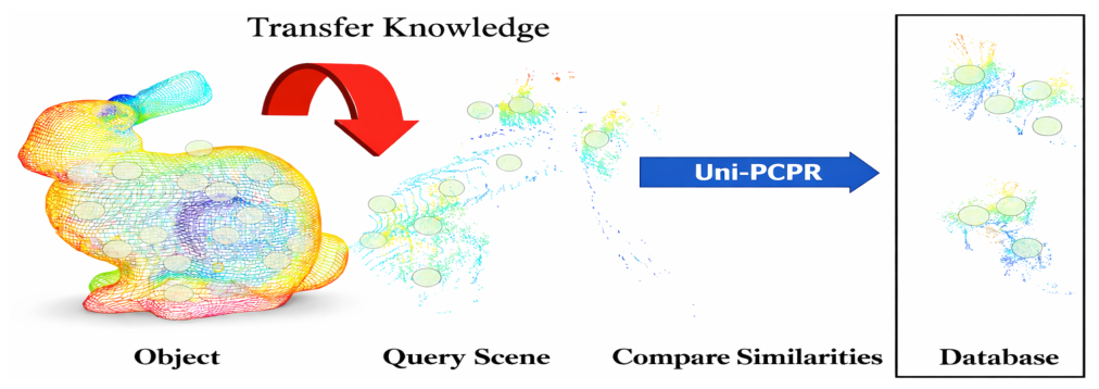
Figure 2.
In Uni-PCPR we use the farthest point sampling to determine the centers and k-nearest neighbors to form the patches. For illustrative purposes, the centers are shown in red. An input is transferred into mini-PointNet and the foundation model to form the tokens that represent the scene. Finally, tokens are aggregated with optimal transport into one global feature vector.
Figure 2.
In Uni-PCPR we use the farthest point sampling to determine the centers and k-nearest neighbors to form the patches. For illustrative purposes, the centers are shown in red. An input is transferred into mini-PointNet and the foundation model to form the tokens that represent the scene. Finally, tokens are aggregated with optimal transport into one global feature vector.
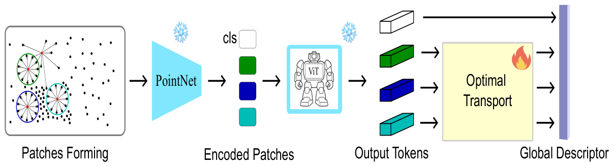
Figure 3.
The evaluation of adapted Uni3D (a pretrained model from other domain) using different numbers of patches and k-neighbors in to form patches.
Figure 3.
The evaluation of adapted Uni3D (a pretrained model from other domain) using different numbers of patches and k-neighbors in to form patches.
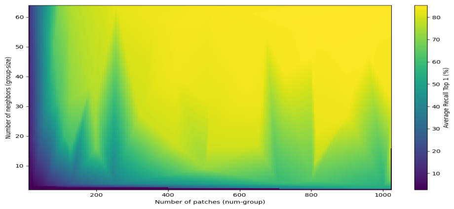
Figure 4.
In this figure, you can see that global geometric awareness is crucial for localization. Point cloud regions with low codensity provide specific local details and can be less important than global awareness.
Figure 4.
In this figure, you can see that global geometric awareness is crucial for localization. Point cloud regions with low codensity provide specific local details and can be less important than global awareness.
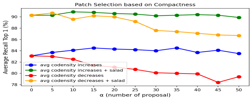

Table 1.
Generalizability comparison on Oxford RobotCar and indoor datasets (Part 1). Methods are evaluated on AR@1% and AR@1 metrics. HeLiOS and Uni-PCPR represent specialized approaches; Uni3D variants show foundational model performance.
Table 1.
Generalizability comparison on Oxford RobotCar and indoor datasets (Part 1). Methods are evaluated on AR@1% and AR@1 metrics. HeLiOS and Uni-PCPR represent specialized approaches; Uni3D variants show foundational model performance.
| Oxford | R.A. | B.D. | ||||
|---|---|---|---|---|---|---|
| Method | AR@1% | AR@1 | AR@1% | AR@1 | AR@1% | AR@1 |
| SOLID | 21.4 | 11.4 | 33.2 | 21.8 | 28.3 | 22.4 |
| PointNetVLAD | 46.4 | 31.6 | 61.6 | 51.0 | 60.9 | 53.8 |
| MinkLoc3Dv2 | 78.0 | 62.3 | 90.7 | 85.7 | 89.5 | 85.9 |
| CASSPR | 44.3 | 30.2 | 49.3 | 40.9 | 48.7 | 43.0 |
| CrossLoc3D | 74.8 | 55.7 | 94.0 | 65.6 | 91.5 | 65.6 |
| HeLiOS | 80.8 | 65.9 | 97.5 | 93.9 | 96.2 | 92.7 |
| Uni-PCPR | 95.7 | 89.0 | 95.5 | 90.3 | 92.7 | 88.4 |
| Uni3D-base | 84.6 | 72.1 | 91.3 | 84.3 | 87.8 | 82.4 |
| Uni3D-tuned | 91.8 | 81.7 | 90.3 | 83.1 | 86.6 | 81.9 |
Table 2.
Generalizability comparison on Oxford RobotCar and indoor datasets (Part 2). Continuation of Table 1 with remaining datasets. Best results per column in bold.
Table 2.
Generalizability comparison on Oxford RobotCar and indoor datasets (Part 2). Continuation of Table 1 with remaining datasets. Best results per column in bold.
| U.S. | CS3D | |||
|---|---|---|---|---|
| Method | AR@1% | AR@1 | AR@1% | AR@1 |
| SOLID | 44.2 | 26.5 | 56.7 | 36.4 |
| PointNetVLAD | 69.4 | 55.9 | 68.8 | 44.6 |
| MinkLoc3Dv2 | 92.4 | 85.0 | 65.7 | 38.2 |
| CASSPR | 55.5 | 44.8 | 58.3 | 37.2 |
| CrossLoc3D | 96.9 | 66.8 | 58.0 | 45.8 |
| HeLiOS | 98.2 | 92.2 | 65.2 | 51.8 |
| Uni-PCPR | 98.3 | 92.4 | 63.6 | 50.2 |
| Uni3D-base | 95.6 | 86.4 | 57.8 | 45.0 |
| Uni3D-tuned | 94.7 | 87.9 | 59.1 | 48.2 |
Disclaimer/Publisher’s Note: The statements, opinions and data contained in all publications are solely those of the individual author(s) and contributor(s) and not of MDPI and/or the editor(s). MDPI and/or the editor(s) disclaim responsibility for any injury to people or property resulting from any ideas, methods, instructions or products referred to in the content. |
© 2026 by the authors. Licensee MDPI, Basel, Switzerland. This article is an open access article distributed under the terms and conditions of the Creative Commons Attribution (CC BY) license (http://creativecommons.org/licenses/by/4.0/).
Copyright: This open access article is published under a Creative Commons CC BY 4.0 license, which permit the free download, distribution, and reuse, provided that the author and preprint are cited in any reuse.