

Submitted:
24 May 2026
Posted:
25 May 2026
You are already at the latest version
Abstract
The formation and development of gullies is a pervasive driver of hillslope degradation, yet forecasting where and at what elevation gullies begin remains challenging. This study proposes a morphometric–energetic framework to anticipate gully initiation zones in catchments developed on low-permeability lithologies and limited tectonic control, across contrasting climatic and geomorphic settings. Using GIS analyses and morphometric parameters, some of these derived from hypsometric curves, our objective is to link basin-scale morphology and energy distribution to the propensity for linear incision, thereby defining an altitudinal belt and stream network positions most susceptible to gully initiation. The framework is designed to be quantitative, transferable among landscapes, and parsimonious in data requirements. By prioritizing diagnostics that can be computed from standard topographic datasets, the approach aims to support land-use planning and sediment-risk mitigation, offering a practical pathway for early identification and management of areas vulnerable to gullying.
Keywords:
gully erosion
; hypsometric curve
; morphometric analysis
; water energy potential
1. Introduction
Linear erosion processes, particularly those caused by concentrated overland flow, are widely recognized as one of the dominant mechanisms behind global land degradation. These processes involve the removal of soil along preferential flow paths, leading to channel incision and the formation of rills and gullies. In the context of the Anthropocene, such erosive dynamics have intensified dramatically. This escalation is primarily attributed to the combined influence of climate change, land use shifts (e.g., deforestation, urbanization, and agricultural expansion), and unsustainable land management practices (Morgan, 1995; Poesen et al., 2003; Valentin et al., 2005; Webster, 2005). Among the various forms of linear erosion, gully erosion stands out for its severity and geomorphic impact. It represents an advanced stage of surface incision where ephemeral or permanent channels become deeply entrenched, often irreversibly altering the hydrological and sediment transport regimes of catchments. Gully erosion not only results in substantial topsoil loss and reduced land productivity but also poses a significant threat to downstream environments by contributing disproportionately to sediment yields. Empirical studies indicate that gully systems can contribute up to 90% or more of the total sediment load delivered by fluvial systems, especially in degraded or semi-arid landscapes (Dube et al., 2020; García-Ruiz et al., 2013, 2015; Hooke, 2000; Huon et al., 2005; Krause et al., 2003; Poesen et al., 2003; de Vente and Poesen, 2005; Wasson et al., 2002). This type of erosion is further exacerbated by the increasing frequency of extreme rainfall events, linked to global climate variability, which enhances runoff generation and stream power.
Despite their recognized environmental and geomorphological importance, linear erosion processes, such as rill and gully formation, have historically received significant scientific attention but yielded limited results particularly regarding their initiation mechanisms and temporal evolution. This research gap is mainly attributable to the intrinsic complexity of these processes, which involve a broad range of interacting geomorphological, hydrological, and pedological factors. The genesis and dynamics of gully systems, in particular, are influenced by variables such as rainfall intensity, soil erodibility, slope morphology, vegetation cover, and anthropogenic disturbances. These factors are difficult to quantify and integrate into reliable predictive models. As highlighted by several authors (Gomez et al., 2003; Sidorchuk, 2006; Siepel et al., 2002; Torri et al., 2018), the lack of consistent field data, along with the spatial heterogeneity of erosion-prone areas, has posed significant challenges to model calibration and validation.
To address this complexity, morphometric analysis has emerged as one of the earliest and most robust quantitative frameworks for interpreting the form and function of drainage basins. By quantifying key metrics such as drainage density, stream frequency, bifurcation ratio, relief, and hypsometric integral, morphometric studies provide insight into catchment erosional maturity, sediment transport potential, and susceptibility to linear erosion. The foundation of this approach can be traced back to the seminal work of Horton (Horton, 1945, 1932), who pioneered the mathematical characterization of drainage networks and set the stage for the evolution of modern geomorphometry.
Subsequent advancements by researchers such as Strahler (Strahler, 1952, 1964), (Leopold et al., 1964; Schumm, 1956), significantly expanded the theoretical and methodological framework, enabling more refined assessments of basin evolution and erosional energy. These methods are now complemented by GIS and remote sensing technologies, which have revolutionized morphometric research by enabling high-resolution, spatially explicit analysis across large, inaccessible terrains.
Topographic parameters, particularly the relationship between local slope gradient (S) and drainage area (A), have proven to be key indicators in understanding the spatial initiation and development of gully erosion. Numerous studies have highlighted how this S–A relationship effectively governs the location of gully heads across a wide range of geomorphic settings, especially in hillslopes subject to diffused hydrological and erosive pressures (Li et al., 2004; Montgomery and Dietrich, 1992; Poesen et al., 2003; Torri and Poesen, 2014; Wu and Cheng, 2005). This relationship is often expressed through threshold equations of the form ; where the coefficient and the exponent are empirically derived and reflect local environmental conditions, such as lithology, vegetation cover, rainfall intensity, and land use (Montgomery and Foufoula-Georgiou, 1993; Tucker et al., 2001). Recent applications of this model, have yielded specific threshold curves that delineate the critical conditions under which concentrated overland flow transitions into channelized erosion, providing valuable predictive insights for erosion risk mapping and landscape evolution modeling.
This study follows a previous research conducted by the same authors (Ciccolini et al., 2024). Using an original morphometric approach and basic GIS tools, they identified the transition between catchment sectors with different erosive capacities of running water, confirming Strahler’s (Strahler, 1952) insigth about the important geomorphological role of the inflection point of the hypsometric curve.
The above approach has been applied on 35 sample basins across three test areas: one in central Italy, another in the Mountain States (U.S.A., Wyoming) and a third in New Zealand. All these basins are characterized by different climatic, morphometric, geomorphological and land-use conditions, as well as different degrees of anthropization; the only similarities are the less permeable bedrock, which allows the formation of a well-developed hydrographic network, and the low degree of tectonic conditioning.
The study also demonstrates that the triggering altitude of the deepening processes (gullies) is strictly related to the basin’s mean elevation and, among other things, to the relative maximum of the energy potential distributed downwards from the watershed.
2. Materials and Methods
2.1. Study Areas
In this study, as already mentioned, 35 sample basins were selected in three study areas from three different continents (North America—USA, Europe—Italy, and Oceania—New Zealand) (Figure 1); this choice was motivated by the desire to test the proposed methodology in areas characterised by different geomorphological and climatic conditions, but with a similar low permeability bedrock and a low degree of tectonic conditioning.
2.1.1. Area 1—North America
The first study area covers a sector of about 2100 km2 within the Gillette coalfield in northeastern Wyoming (Figure 2a). The landscape is defined by a broad highland with gentle ridges and limited elevation differences, ranging between 1400 and 1500 m a.s.l. Human impact in the area is minimal, restricted to scattered buildings mainly located across the plains; the slopes remain largely uncultivated, with sparse vegetation (predominantly shrubs) concentrated within river valleys. The bedrock is relatively homogeneous, consisting primarily of Paleocene and Eocene siltstones and shales, locally overlain by weathered silty-clay deposits (especially on hilltops and ridges) or fine colluvium (Luppens et al., 2008; Robinson et al., 1964). Stratigraphically, these formations exhibit a highly regular structure, with nearly continuous, horizontal layers and little to no tectonic influence.
Due to its elevation, this part of Wyoming experiences a relatively cool and arid climate, with average annual maximum temperatures around 15 °C and minimum values close to 1 °C. The presence of mountain ridges that intercept humid air masses from the Pacific Ocean contributes to the generally low precipitation levels, averaging between 400 and 450 mm per year (US Climate Data, usclimatedata.com). In this sector, gully erosion processes are particularly effective due to the poor soil cover and the near absence of tall vegetation (Figure 2b).
2.1.2. Area 2—Central Italy
This area covers a sector of about 1200 km2 on the Adriatic side of central Italy (Figure 3a). It is characterised by a predominantly high-hilly and hilly landscape with altitudes (generally below 500–600 m a.s.l.) that decrease progressively eastward to the coastal belt. The slopes are mainly used for agriculture, while small urban settlements and inhabited centres are mainly located along the watersheds. The essentially homogeneous bedrock is characterised by Plio-Pleistocene formations consisting of alternating shale and sandy-conglomeratic layers (Centamore and Deiana, 1986; Gentili et al., 2017); these formations are locally covered by medium-fine continental deposits (colluvial and/or fluvial). The structural framework of the Plio-Pleistocene formations is expressed at the surface as a regular, eastward-dipping monocline, formed as a result of the regional tectonic uplift that began in the Early Pleistocene (D’Agostino et al., 2001). Overall, the monoclinal structure is offset by a few dip-slip faults, mainly oriented NNW–SSE and WSW–ENE, with displacements rarely exceeding 10 m (Gentili et al., 2017). These tectonic features, however, do not produce significant morphological evidence at the surface, nor do they exert a notable influence on the hydrographic network.
From a climatic perspective, the area represents a transition zone between the Mediterranean climate, typical of southern Italy, and the humid subtropical (or temperate oceanic) climate, which is widespread across much of the territory (Gentilucci et al., 2020, 2021). The study area records an average annual temperature of about 14 °C, with maximums in July and August and minimums in January. Precipitation ranges from around 600 mm along the coast to 1000 mm in the higher hilly sector. The relationship between temperature and rainfall indicates a slight summer aridity in the low-hilly and coastal zones from July to mid-September. Under these conditions, gully erosion processes are fairly common (Buccolini et al., 2014; Gentili et al., 1998), although dense perifluvial vegetation (Figure 3b) sometimes obscures their activity. On the other hand, this vegetation makes the transition between these processes and the slope areas dominated by widespread rill erosion more clearly visible.
2.1.3. Area 3—New Zealand
The third study area covers two different sectors, totaling approximately 400 km2 on the eastern side of the North Island, New Zealand (Figure 4a and b). The landscape, in general is characterised by a typical high-hilly terrain with altitudes between 200 and 600 m a.s.l., which progressively decrease towards the east and the coastal belt. In the northernmost sector land use is dominated by intensive horticulture and viticulture, supported by the region’s highly productive soils and favorable climate, alongside significant areas of pastoral farming, forestry, and increasingly, urban development. In the southernmost sector, the territory is mainly exploited for livestock grazing, primarily sheep and bulls. However, in several areas, the slopes are entirely uncultivated or covered by forests (data from Operative Hastings District Plan at https://eplan.hdc.govt.nz/eplan).
The whole area occupies a now-uplifted part of a late Neogene forearc basin and associated inboard margin of an accretionary wedge, which are all part of the actively deforming Hikurangi subduction margin, inferred to have commenced between 40 and 24 Ma (Bache et al., 2012; Stagpoole and Nicol, 2008). From a lithologic point of view, the bedrock in the northernmost sector is mainly characterized by the presence of alternating mudstones sandstones and conglomerates belonging to the Mangaheia Group, a shallow-marine, limestone-bearing Pliocene succession up to 1.5 km thick; the southernmost sector, on the other hand, is characterized by the presence of prevalent mudstones and sandstones of different age (Cretaceous to Miocene). Despite the complex geological setting, its influence on the hydrographic network and, in general, on surface geomorphological processes appears rather limited (Bland et al., 2019).
Sheltered by the mountain ranges to the west, this area benefits from a predominantly dry and sunny climate. Summer is usually characterized by warm, stable, and dry weather, while during winter frost may occasionally occur. Typical daytime maximum temperatures in summer range between 20 °C and 28 °C, with occasional peaks above 30 °C. High heat is a common feature of the season and can be intensified by strong, dry föhn winds blowing from the northwest. Extreme values up to 39 °C have been recorded. In winter, conditions are milder in the northern part of the region and cooler in the southern areas, with usual daytime highs between 10 °C and 16 °C. Heavy rainfall can develop under easterly or southeasterly flows (data from National Institute of Water and Atmospheric Research-NZ at https://niwa.co.nz/). In such conditions gully erosion is widespread (Figure 4c), affecting some 10% of the land area (Eyles, 1985).
3. Methodology
The study has been organized in several steps:
- -
- Calculation of the basic morphometric parameters of all the subbasins.
- -
- Construction of the hypsometric curve.
- -
- Analytical determination of the energy potential of running waters within the individual subbasin.
- -
- Calculation of Şen’s “energy index” (Şen, 2019) for gully head formation.
- -
- Detection of gully heads within the sample basins through satellite image interpretation.
3.1. Calculation of the Basic Morphometric Parameters of All the Subbasins
Basic morphometric parameters have been calculated using the ArcGIS Pro software (ESRI, v.3.5.3) and using DTMs with a resolution of 10 m; the latter can be downloaded free of charge from the links https://doi.org/10.13127/tinitaly/1, https://portal.opentopography.org/, and https://maps.gns.cri.nz/ for the Italian, US, and New Zealand catchments, respectively. Selecting a DTM with an appropriate resolution is a crucial aspect. Today, global datasets of comparatively high resolution are accessible (around 10–30 m), while local or regional sources, such as LiDAR, can provide even finer detail. Our primary objective was to use the highest-resolution DTMs available, but also to design a processing approach adaptable to a wide DTM represents an excellent option for morphometric analysis (Ciccolini et al., 2024; Fornaciai et al., 2012; Vörös et al., 2022). In this study, we deliberately did not use 1 m resolution LiDAR data, as they can generate “false” elevation variations in semi-urbanized areas, often caused by features such as roads or pathways (Ciccolini et al., 2024). These anomalies may introduce inaccuracies in GIS-based determination of “flow direction”.
After acquiring the DTMs and refining them by clipping along the basin boundaries, we removed all sinks using the “Fill tool” (Spatial Analyst) to obtain “hydrologically” correct DTMs. We then calculated a series of basic morphometric parameters, including area, perimeter, mean slope, maximum and minimum elevation, and the “Circularity ratio”, defined as the ratio between the basin area and that of a circle with the same perimeter (Miller, 1953). The drainage network was classified using the (Strahler, 1957) method, which assigns orders to streams based on their hierarchy. From the reconditioned DTM, flow direction and flow accumulation rasters were generated in GIS, with a 10-cell threshold applied to define the stream network. Finally, the ArcGIS “Stream Order” and “Stream to Feature” tools were used to produce stream order rasters and polyline features representing river reaches by order.
After defining the hydrographic network, we produced a flow contribution curve (FCC, Ciccolini et al., 2024) for each stream order, showing the number of river segments distributed across different elevations. This value, denoted as Nuz, corresponds to the number of stream sections intercepted at a given elevation z (Figure 5a). It was obtained by counting the intersections between the hydrographic network vector file and the contour lines extracted from the DTM (Figure 5b), with a contour interval set at 10 m for consistency with previously derived parameters. Therefore, we represented the number of reaches by order (Nuz_I for first-order streams, Nuz_II for second-order, etc.), which allowed us to analyze the distribution and quantity of reaches at different elevations; to make this representation comparable with other parameters described later, we generated semi-dimensional curves with normalised basin area values (a/A between 0 and 1, Figure 5c). This graphical representation highlights elevation ranges corresponding to peak values, which indicate where fluvial erosion was particularly effective. Finally, we calculated the mean of the contribution areas upstream of the third-order streams obtained previously. As will be explained in detail below, this can be considered the area necessary for the activation of significant erosive processes.
3.2. Construction of the Hypsometric Curve
To estimate the mean elevation of each basin and compare the previously obtained FCC trends, we constructed the hypsometric curves (Strahler, 1952), using the ArcGIS “CalHypso” tool (Pérez-Peña et al., 2009); These curves represent the proportion of basin area above a given elevation. Typically expressed in non-dimensional form (relative height h/H vs. relative area a/A), these curves allow comparison among different basins. For this study, to better highlight correlations between other relative elevations, we also created semi-dimensional curves with normalized basin area values (Figure 6). The hypsometric curve, modeled with a 3rd-degree polynomial, identifies two oblique inflection points (OIPs): one within the basin, where slope energy shifts from rapid to slower mass loss (Strahler, 1952), and another outside the diagram, which is only a mathematical solution with no physical meaning, as it lies below the basin outlet. These special points are therefore calculated for each subbasin.
3.3. Analytical Determination of the Energy Potential of Running Waters Within the Individual Subbasin
The hypsometric curve can also be used to define the energy potential of each point within a drainage basin. Starting from simple physical-mathematical relationships, it is known that if a water particle of mass m moves without friction and descends by a value dh, by the principle of conservation of potential and kinetic energy, we have:
where is the velocity (L/T) and is the gravitational acceleration (L/T2).
Simplifying for , once the square of the binomial has been developed at the second term, and taking into account that the quantity is very small and can be neglected we obtain:
Integrating the two terms of the equation, respectively in and in , we have:
Finally, substituting v in the formula for the power (), where F is the force we have:
This formula tells us that in the hypsometric curve for , the power and that for , with expressed in watts. Evidently, this is an “ideal” system that does not take into account the energy dissipated by friction, but in absolute terms, it can be compared with the morphometric evaluations.
To apply the method to each basin in GIS, we used the following procedure. Starting from the DTM (10m resolution, Figure 7a), a raster of the h/H values of the hypsometric integral, divided into 20 classes between 0 and 1 (Figure 7b) and a raster of the slope in radians (Figure 7c) were created. Applying the formula, a raster of the power P values per unit mass m is obtained (Figure 7d).
3.4. Calculation of Şen’s “Energy Index” for Gully Head Formation
The value of the power , although significant, cannot be directly related to the relationship between height and relative area (such as in a hypsometric curve) and energy in a drainage basin.
One possible solution is to use a method commonly used to measure the electric potential in a drainage basin (for example, in the presence of a dam). The “single-point” method, which relates the hydroelectric energy , the specific density of water , the flow rate , and the head , is the most widely used alternative (Şen, 2019).
This approach does not take into account the difference in elevation of the drainage basin, but depends only on the water height at a single point along the main drainage channel. Theoretically, the differences in power gain , elevation , and flow rate can be obtained from the Equation 6:
One way to relate discharge to basin area and the “energy” of the water, such as rainfall intensity, is to use a formula like the Rational Method (Cronshey, 1986), a simple but widely used hydrological technique for estimating peak discharge from small drainage basins. It relates rainfall intensity (), catchment area (), and a runoff coefficient () to calculate the maximum flow rate ().
Substituting these terms into Equation (6) we get:
If we assume the density of water is 1, the runoff coefficient is 1 (considering only the drainage area and altitude, without geological influences), and the rainfall intensity is also 1 (i.e., the drainage basin, effective over the entire area, can be adjusted according to rainfall intensity), we can write
The product of the infinitesimal increase in drainage area and the decrease in elevation is defined as the Energy Index () of the drainage basin (Şen, 2022), where hydrometeorological and geological effects play no role. In practice, Ei can be defined as the infinitesimal energy per unit density of a basin subjected to constant rainfall intensity and a unit runoff coefficient.
The Energy Index can therefore be easily adapted to the hypsographic curve of a basin by normalising the values of the heights and the relative contributing areas to 1.
This approximation allows us to consider the energy associated with the action of surface running water within a hydrographic basin in absolute terms and, consequently, to compare basins of very different sizes and morphometric characteristics.
3.5. Detection of Gully Heads Within the Sample Basins Through Satellite Image Interpretation
The correspondence between the results of the analytical procedures described above and the presence on the field of erosive processes linked to gullies, was verified using high-resolution satellite images from Google Earth (© Google, 2025); data sources include Landsat/Copernicus and Maxar Technologies.
More specifically, within each river basin, the gully heads were selected (Figure 8a and b) and a 20% trimmed mean of the relative elevations was obtained in order to exclude anomalous values linked to possible (although minimal as mentioned in the introduction to this study) influences of anthropogenic and/or geological-structural origin on the development of these processes.
4. Results
The results of the steps a, b, and e described above are summarized in Table 1. By comparing some parameters obtained from the analysis it is possible to identify relatively narrow sectors within each catchment that can be directly linked to the erosive processes associated with surface running waters. The graphs in Figure 9. for nine sample catchments (three from each study area) show, in semi-dimensional form, the FCCs for the first three order reaches and the corresponding hypsometric curve. The FCCs all display a general bell-shaped distribution with respect to elevation, indicating that the greatest number of network segments develop in relatively limited sectors of the catchment. The highest-order reaches (second- and third-order) also exhibit more pronounced peaks corresponding to specific heights within the catchment. Once the hypsometric curve was plotted, it was possible to determine two further heights: the mean basin height (Hmean in Table1, dashed light green line in the graph) and the corresponding OIP (oblique inflection point). As shown in the graphs, these two elevations and the one corresponding to the most pronounced peak of the FCCs (generally that of the third-order reaches—dashed red line, Hmean_III FCC in Table1) have very similar values, in some cases almost coinciding; this specific stream order, as mentioned above, is purely indicative since it is known to depend on the scale of representation. Even the standard deviation σ calculated for the “heights” of each basin is consistently below or around 10 m (the acceptable error for the resolution of the chosen DTM); only five of the selected basins show a standard deviation between 15 and 20 m. The dashed black line, on the other hand, indicates the mean height of the gullies identified through satellite imagery analysis (Hmean_gullies field in Table 1). In most of the analyzed basins, this elevation is very close to those described previously, while in some it differs by even a few dozen meters, as in the case of basin 1 within Area 1 (USA), or basins 3 and 8 in Area 2 (Italy).
This apparent discrepancy, as will be explained in more detail later in the manuscript, may be associated with local “inhomogeneities” of lithological and/or structural or anthropogenic origin within the individual basin.
The data on the mean contribution areas of the III-order reaches (Amean_III contr in Table 1) are also very interesting; all these areas fall within a relatively narrow range, with values between 10,000 and 20,000 m2 (between 1 and 2 hectares).
The results of the analyses described above enable us to identify, as mentioned, specific sectors within a catchment area where processes related to surface running waters are concentrated. However, these assessments are essentially based on morphometric analyses or direct observations, without any information on the energy required to activate these processes. The calculation procedure described in point c) of the previous paragraph, therefore, enables us to identify the sectors of the catchment characterised by the highest values of water potential energy (in terms of power per unit mass). Observing the results (some examples are shown in Figure 10), the correspondence between the maximum energy values and the areas of gully activation within the catchments is very clear.
Equally significant is the fact that these sectors are generally located at the mean height of the catchment area, as calculated from the hypsometric curve. This correspondence, therefore, allows us to link the energy to the other “elevations” determined with a semi-quantitative procedure from the morphometric analyses. However, the power P value (in watts), while providing a quantitative indication of the energy of the water at each point in a generic hydrographic basin, is actually a function of parameters such as the mass and slope of the basin and cannot be treated in absolute terms as a function of the hypsometric curve trend.
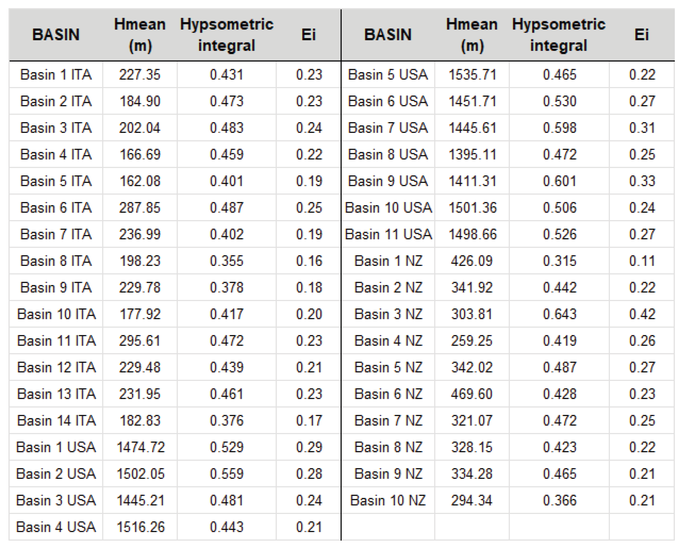
The Şen’s “Energy Index” Ei, on the other hand, by using normalized (between 0 and 1) areas and elevations allows to compare basins of very different sizes and morphometric characteristics. Table 2 presents the Ei values for all 35 basins analysed, alongside their respective mean height values.
Examining the results, the average Ei value is 0.24, with a small standard deviation of 0.05. Specifically, the interquartile range (IQR)—the interval between the 25th and 75th percentiles, which indicates the width of the central band of the data—yields a value of 0.045; consequently, this band lies between 0.21 and 0.25. The significance of this result is also highlighted from a statistical perspective; it is noteworthy that the Ei values follow a normal distribution (Figure 11a), confirming the high probability of observing a certain range of values. Similar indications are evident from the frequency distribution graph (Figure 11b), which clearly shows that the majority of values are concentrated within a relatively narrow band.
The Ei values obtained fall within the “Low” class as defined by (Şen, 2022), who classifies Energy Index values into five categories, from very low to very high (ranging between 0 and 1). However, this classification originates from studies evaluating the hydroelectric potential of river basins. As it is necessary to define a minimum energy required to activate erosive processes, the obtained Ei values in this study can be considered largely justified.
Very interesting information can be obtained by comparing the Energy Index values with other basin morphometric parameters. As shown in the graph in Figure 12a, there is a close correlation between Ei and the hypsometric integral while there is no correlation between the Energy Index and basin area, basin slope, mean height or circularity ratio (Figure 12 b, c, d, and e).
5. Discussion
The analyses described in the previous paragraphs provide valuable and original insights for defining, within a generic river basin, the areas most susceptible to triggering “intense” erosion processes (i.e., gully-type erosion).
One of the most notable findings is the strong correlation between heights calculated using different methods (i.e., satellite imagery, GIS, and statistical analyses) and the mean heights derived from hypsometric curves (Table1). The standard deviation (σ), as noted in the previous paragraph, generally remains below or around 10–15 metres, which is an acceptable margin of error given the resolution of the used DTM. Of the five σ values above 15, four are found in Italian basins, which, compared to the other two selected areas, are characterised by a higher degree of anthropisation. The inclusion of the “height” corresponding to the activation of third-order reaches among these is considered a secondary aspect, influenced solely by the resolution of the DTM (Ciccolini et al., 2024). However, this hierarchical order remains consistent across the basins in all the test areas and appears unaffected by the main morphometric parameters of the basins (such as area, perimeter, shape, slope, etc.).
The observed similarities can be explained by the fact that gullies constitute the prevailing morphodynamic mechanism in the highest parts of the basins. Accordingly, the hypsometric curves display the OIPs, where the curve shifts from concave to convex, at essentially the same elevation. These inflection points mark a threshold between low-intensity, areal erosion (sheet and rill) and deep incision processes (gully formation), and likely correspond to the elevation at which the greatest decline in potential energy is coupled with the greatest rise in kinetic energy. This concept was already noted by (Strahler, 1952), who identified a transition between zones with relatively higher and lower mass-change rates.
Another interesting finding from the study is that the contributing areas upstream of the third-order streams in all basins exhibit comparable characteristics. Calculating the mean contributing areas for the reaches discussed above (Amean_III contr) reveals a consistent pattern: despite belonging to basins that vary widely in size and morphometric traits, these areas cluster within a relatively narrow interval, about 10,000–20,000 m2 (1–2 ha; Table1). Given the distinct rainfall regimes characterizing the three test areas, this similarity is pivotal for interpreting slope-scale erosion mechanisms, as it allows the “position” factor to be treated as the sole effective driver of these processes. Although identifying topographic thresholds for gully-head development is well established in the literature, where threshold conditions are typically expressed as log–log relationships between slope area (A) and slope gradient (S), the procedure adopted here produced valuable values although not always comparable (Ciccolini et al., 2024; McNamara et al., 2006; Vandekerckhove et al., 2000; Wu and Cheng, 2005). By contrast, it departs substantially from approaches that rely on composite topographic indices to describe catchment hydro-geomorphology, for example, the RUSLE LS factor (sediment-transport capacity,Moore & Wilson, 1992), the Stream Power Index (SPI) (potential channel erosion,Wilson & Gallant, 2000), the Terrain Characterization Index (TCI) (transport capacity, Park et al., 2001), and the Topographic Wetness Index (TWI) (topographic control on hydrological processes, Conoscenti et al., 2008; Wilson & Gallant, 2000). Such indices often delineate zones susceptible to various erosion and deposition processes, which do not necessarily coincide with the elevation at which gully heads are initiated.
The most interesting innovation of the study, however, is the ability to quantify in terms of energy the process that leads to the activation of gullies or other intense erosive processes. The Şen’s “Energy Index” Ei value, in particular, consistent with what has been highlighted in studies evaluating hydroelectric energy potential in some river basins, allows us to determine which sector of the basin, when expressed as a function of its hypsometric curve, exhibits the highest values. These areas are consistently located in the range close to the mean height, confirming that this elevation represents a key point in the geomorphological evolution of the basin. The values obtained (between 0.21 and 0.25), considered in absolute terms, are purely indicative; when compared with the efficiency classes proposed by (Şen, 2022), they would fall into the “low” class (between 0.1 and 0.3), noting that, as repeatedly mentioned, those classes describe the maximum potential for electricity production. In the case of erosional processes, the energy required is certainly lower, and the values obtained can be considered the minimum energy necessary to initiate them. Further confirmation of the utility of the hypsometric curve for identifying the sectors of a basin most susceptible to the initiation of intense erosional processes is provided from the strong correlation between Ei and the value of the basin’s hypsometric integral. Indeed, higher values are associated with geomorphologically younger basins and, consequently, with greater “residual” erosive potential. No correlation was found when comparing Ei with the basin area, average slope, or mean height, demonstrating that the triggers for these processes are not a function of absolute values but rather of reciprocal values within the individual basin. The lack of correlation between Ei and the basin circularity ratio is also not surprising; this parameter, although directly related to a catchment’s predisposition to produce significant discharge peaks during flood events, does not actually express the energy of the water, but rather the characteristic of the hydrographic network to generate flows with a similar concentration time.
6. Conclusions
The aim of this study was to demonstrate that, by relying solely on morphometric analysis and a digital terrain model of suitable resolution, it is possible to estimate the elevation and average contributing area required to trigger accelerated erosion processes classified as gullies in basins that are relatively homogeneous in lithological terms and only weakly, or not at all, influenced by geological–structural factors. A similar procedure also allows quantification of water potential (Power in watts), and the definition of a dimensionless energy index, normalised as a function of the heights and relative areas within a hydrographic basin. Compared with approaches that require a larger set of parameters and/or targeted field surveys, this method is much more flexible and straightforward to apply, especially given the growing availability of powerful IT tools (GIS) and high-resolution digital terrain models. The findings of this study indicate that gully erosion processes require a minimum energy threshold to begin, and that this threshold can be associated with a specific contributing area or elevation. Consequently, morphometric analysis can be considered an effective and adaptable tool for quickly identifying where erosive processes are likely to occur and, when combined with other methods, for quantifying them and planning soil erosion control measures.
More specifically, the study highlighted that:
- -
- The gully’s triggering altitude, determined through both GIS procedures and satellite image interpretation, corresponds to the basin’s mean height (as indicated by the hypsometric curve) and the highest elevation where the reaches show a peak in their frequency distribution. When a 10 m DTM is used, the elevation typically aligns with the heads of third-order reaches.
- -
- A similar correspondence is found between these relative heights and the more elevated inflection point of each basin’s hypsometric curve. This level also marks the transition from low-intensity erosional processes (sheet and rill erosion) to deep incision (gully formation).
- -
- The contributing area of the basin required to trigger these high-energy erosive processes consistently falls within approximately 1–2 ha, or at least within a narrow range, regardless of the basin’s overall size and morphometric characteristics.
- -
- This characteristic elevation belt can also be expressed in energetic terms, both in absolute units (Power, W) and as a relative metric (Energy index, Ei). The latter provides a value independent of basin area, mean slope, mean elevation, and planimetric shape, making it particularly suitable for comparing basins with markedly different geometries.
Data Availability Statement
The data that support the findings of this study are available on request from the corresponding author. The data are not publicly available due to privacy or ethical restrictions. All data processing necessary to produce the maps was performed using ESRI-ArcGisPRO 3.6.0. The Figures in the document were created using CorelDraw Home&Student 2019.
Conflicts of Interest
The authors declare no conflict of interest.
References
- Bache, F.; Sutherland, R.; Stagpoole, V.; Herzer, R.; Collot, J.; Rouillard, P. Stratigraphy of the southern Norfolk Ridge and the Reinga Basin: A record of initiation of Tonga–Kermadec–Northland subduction in the southwest Pacific. Earth Planet Sci. Lett. 2012, 321–322, 41–53. [Google Scholar] [CrossRef]
- Bland, K. J.; Nicol, A.; Kamp, P. J. J.; Nelson, C. S. Stratigraphic constraints on the late Miocene–Pleistocene evolution of the North Island Fault System and axial ranges in the central Hikurangi subduction margin, New Zealand. New Zealand J. Geol. Geophys. 2019, 62, 248–272. [Google Scholar] [CrossRef]
- Buccolini, M.; Materazzi, M.; Aringoli, D.; Gentili, B.; Pambianchi, G.; Scarciglia, F. Late Quaternary catchment evolution and erosion rates in the Tyrrhenian side of central Italy. Geomorphology 2014, 204. [Google Scholar] [CrossRef]
- Centamore, E. and Deiana, G.: LA GEOLOGIA DELLE MARCHE, edited by: Univerisità di Camerino, D. di S. della T., 145 pp., 1986.
- Ciccolini, U.; Bufalini, M.; Materazzi, M.; Dramis, F. Gully Erosion Development in Drainage Basins: A New Morphometric Approach. Land 13, 792. [CrossRef]
- Conoscenti, C.; Di Maggio, C.; Rotigliano, E. GIS analysis to assess landslide susceptibility in a fluvial basin of NW Sicily (Italy). Geomorphology 2008, 94. [Google Scholar] [CrossRef]
- Cronshey, R. Urban Hydrology for Small Watersheds (No.55); US Department of Agriculture, Soil Conservation Service, Engineering Division, 1986. [Google Scholar]
- D’Agostino, N.; Jackson, J. A.; Dramis, F.; Funiciello, R. Interactions between mantle upwelling, drainage evolution and active normal faulting: an example from the central Apennines (Italy). Geophys J. Int. 2001, 147, 475–497. [Google Scholar] [CrossRef]
- Dube, H. B.; Mutema, M.; Muchaonyerwa, P.; Poesen, J.; Chaplot, V. A global analysis of the morphology of linear erosion features. Catena (Amst) 2020, 190. [Google Scholar] [CrossRef]
- Eyles, G. O. 1985. The New Zealand Land Resource Inventory Erosion Classification Edizione 85 di Water & soil miscellaneous publication. In National Water and Soil Conservation Authority. 60 pp.
- Fornaciai, A.; Favalli, M.; Karátson, D.; Tarquini, S.; Boschi, E. Morphometry of scoria cones, and their relation to geodynamic setting: A DEM-based analysis. J. Volcanol. Geotherm. Res. 2012, 217–218. [Google Scholar] [CrossRef]
- García-Ruiz, J. M.; Nadal-Romero, E.; Lana-Renault, N.; Beguería, S. Erosion in Mediterranean landscapes: Changes and future challenges. Geomorphology 2013, 198, 20–36. [Google Scholar] [CrossRef]
- García-Ruiz, J. M.; Beguería, S.; Nadal-Romero, E.; González-Hidalgo, J. C.; Lana-Renault, N.; Sanjuán, Y. A meta-analysis of soil erosion rates across the world. 2015. [Google Scholar] [CrossRef]
- Gentili, B.; Materazzi, M.; Pambianchi, G.; Scalella, G.; Aringoli, D.; Cilla, G.; Farabollini, P. The slope deposits of the Ascensione Mount (Southern Marche, Italy). In Geografia fisica e dinamica quaternaria; 1998. [Google Scholar]
- Gentili, B.; Pambianchi, G.; Aringoli, D.; Materazzi, M.; Giacopetti, M. Pliocene-Pleistocene geomorphological evolution of the Adriatic side of Central Italy. Geol. Carpathica 2017, 68, 6–18. [Google Scholar] [CrossRef]
- Gentilucci, M.; Materazzi, M.; Pambianchi, G.; Burt, P.; Guerriero, G. Temperature variations in Central Italy (Marche region) and effects on wine grape production. Theor. Appl. Climatol. 2020, 140. [Google Scholar] [CrossRef]
- Gentilucci, M.; Bufalini, M.; D’aprile, F.; Materazzi, M.; Pambianchi, G. Comparison of data from rain gauges and the IMERG product to analyse precipitation in mountain areas of central Italy. ISPRS Int. J. Geoinf. 2021, 10. [Google Scholar] [CrossRef]
- Gomez, B.; Banbury, K.; Marden, M.; Trustrum, N. A.; Peacock, D. H.; Hoskin, P. J. Gully erosion and sediment production: Te Weraroa Stream, New Zealand. Water Resour. Res. 2003, 39. [Google Scholar] [CrossRef]
- Hooke, R.L. On the history of human as geomorphic agents. Geology 2000, 28. [Google Scholar] [CrossRef]
- Horton, B. Y. R. E.: MORPHOLOGY, 56, 275–370, 1945.
- Horton, R. E. Drainage-basin characteristics. Eos Trans. Am. Geophys. Union 1932, 13, 350–361. [Google Scholar] [CrossRef]
- Huon, S.; Bellanger, B.; Bonté, P.; Sogon, S.; Podwojewski, P.; Girardin, C.; Valentin, C.; de Rouw, A.; Velasquez, F.; Bricquet, J.-P.; et al. Monitoring Soil Organic Carbon Erosion with Isotopic Tracers: Two Case Studies on Cultivated Tropical Catchments with Steep Slopes (Laos, Venezuela). Soil. Eros. Carbon Dyn. 2005, 301–328. [Google Scholar] [CrossRef]
- Krause, A. K.; Franks, S. W.; Kalma, J. D.; Loughran, R. J.; Rowan, J. S. Multi-parameter fingerprinting of sediment deposition in a small gullied catchment in SE Australia. Catena (Amst) 2003, 53. [Google Scholar] [CrossRef]
- Leopold, L. B.; Wolman, M. G.; Miller, J. P. Fluvial processes in geomorphology; Dover Publications, Inc: New York, NY, 1964; 544 pp. [Google Scholar]
- Li, G.; Klik, A.; Wu, F. Gully erosion features and its causes of formation on the (Yuan) land in the Loess Plateau, China. In Gully Erosion Under Global Change; Li, Y., Poesen, C. V. J., Eds.; Sichuan Science and Technology Press: Chengdu, China, 2004; pp. 131–142. [Google Scholar]
- Luppens, J. A.; Scott, D. C.; Haacke, J. E.; Osmonson, L. M.; Rohrbacher, T. J.; Ellis, M. Assessment of Coal Geology, Resources, and Reserves in the Gillette Coalfield, Powder River Basin, Wyoming. Geol. Surv. Open-File Rep. 2008, 1202, 1–127. [Google Scholar]
- McNamara, J. P.; Ziegler, A. D.; Wood, S. H.; Vogler, J. B. Channel head locations with respect to geomorphologic thresholds derived from a digital elevation model: A case study in northern Thailand. For Ecol. Manag. 2006, 224. [Google Scholar] [CrossRef]
- Miller, V. A quantitative geomorphic study of drainage basin characteristics in the Clinch mountain area, Virginia and Tennessee; Department of Geology Columbia University: New York, 1953. [Google Scholar]
- Montgomery, D. R.; Dietrich, W. Channel initiation and the problem of landscape scale. Science 1992, 255. [Google Scholar] [CrossRef]
- Montgomery, D. R.; Foufoula-Georgiou, E. Channel network source representation using digital elevation models. Water Resour. Res. 1993, 29, 3925–3934. [Google Scholar] [CrossRef]
- Moore, I. D.; Wilson, J. P. Length-slope factors for the revised universal soil loss equation: simplified method of estimation. J. Soil. Water Conserv 1992, 47, 423–428. [Google Scholar] [CrossRef]
- Morgan, R. Soil Erosion and Conservation, 2nd Edition; Longman Group: Essex, 1995. [Google Scholar]
- Park, S. J.; McSweeney, K. K.; Lowery, B. Identification of the spatial distribution of soils using a process-based terrain characterization. Geoderma 2001, 103. [Google Scholar] [CrossRef]
- Pérez-Peña, J. V.; Azañón, J. M.; Azor, A. CalHypso: An ArcGIS extension to calculate hypsometric curves and their statistical moments. Applications to drainage basin analysis in SE Spain. Comput Geosci. 2009, 35, 1214–1223. [Google Scholar] [CrossRef]
- Poesen, J.; Nachtergaele, J.; Verstraeten, G.; Valentin, C. Gully erosion and environmental change: Importance and research needs. In Catena; 2003. [Google Scholar] [CrossRef]
- Robinson, C. S.; Mapel, W. J.; Bergendahl, M. H. Stratigraphy and structure of the northern and western flanks of the Black Hills uplift, Wyoming, Montana, and South Dakota. 1964. [Google Scholar] [CrossRef]
- Schumm, S. Evolution of drainage systems and slopes in badlands at Perth Amboy, New Jersey. Bull. Geol. Soc. Am. 1956, 67. [Google Scholar] [CrossRef]
- Şen, Z. Innovative methodologies in renewable energy: A review. Int. J. Energy Res. 2019, 43, 5621–5658. [Google Scholar] [CrossRef]
- Şen, Z. Hydroelectric energy potential classification via hypsographical curve concept. Int. J. Energy Res. 2022, 46, 20425–20436. [Google Scholar] [CrossRef]
- Sidorchuk, A. Stages in gully evolution and self-organized criticality. Earth Surf. Process Landf. 2006, 31, 1329–1344. [Google Scholar] [CrossRef]
- Siepel, A. C.; Steenhuis, T. S.; Rose, C. W.; Parlange, J. Y.; McIsaac, G. F. A simplified hillslope erosion model with vegetation elements for practical applications. J. Hydrol. (Amst) 2002, 258. [Google Scholar] [CrossRef]
- Stagpoole, V.; Nicol, A. Regional structure and kinematic history of a large subduction back thrust: Taranaki Fault, New Zealand. J. Geophys Res. Solid Earth 2008, 113. [Google Scholar] [CrossRef]
- Strahler, A. Hypsometric (area-altitude) analysis of erosional topography. Bull. Geol. Soc. Am. 1952, 63, 1952. [Google Scholar] [CrossRef]
- Strahler, A. Quantitative analysis of watershed geomorphology. Eos Trans. Am. Geophys. Union 1957, 38, 913–920. [Google Scholar] [CrossRef]
- Strahler, A. Quantitative Geomorphology of Drainage Basins and Channel Networks; Applied Hydrology: New York, 1964; pp. 439–476. [Google Scholar]
- Torri, D.; Poesen, J. A review of topographic threshold conditions for gully head development in different environments. Earth Sci. Rev. 2014, 130, 73–85. [Google Scholar] [CrossRef]
- Torri, D.; Poesen, J.; Rossi, M.; Amici, V.; Spennacchi, D.; Cremer, C. Gully head modelling: A Mediterranean badland case study. Earth Surf. Process Landf. 2018, 43, 2547–2561. [Google Scholar] [CrossRef]
- Tucker, G. E.; Catani, F.; Rinaldo, A.; Bras, R. Statistical analysis of drainage density from digital terrain data. Geomorphology 2001, 36, 187–202. [Google Scholar] [CrossRef]
- Valentin, C.; Poesen, J.; Li, Y. Gully erosion: Impacts, factors and control. Catena (Amst) 2005, 63, 132–153. [Google Scholar] [CrossRef]
- Vandekerckhove, L.; Poesen, J.; Oostwoud Wijdenes, D.; Nachtergaele, J.; Kosmas, C.; Roxo, M. J.; de Figueiredo, T. Thresholds for gully initiation and sedimentation in Mediterranean Europe. Earth Surf. Process Landf. 2000, 25, 1201–1220. [Google Scholar] [CrossRef]
- de Vente, J.; Poesen, J. Predicting soil erosion and sediment yield at the basin scale: Scale issues and semi-quantitative models. Earth Sci. Rev. 2005, 71, 95–125. [Google Scholar] [CrossRef]
- Vörös, F.; de Vries, B. van Wyk; Guilbaud, M. N.; Görüm, T.; Karátson, D.; Székely, B. DTM-Based Comparative Geomorphometric Analysis of Four Scoria Cone Areas—Suggestions for Additional Approaches. Remote Sens. 2022, 14. [Google Scholar] [CrossRef]
- Wasson, R. J.; Caitcheon, G.; Murray, A. S.; McCulloch, M.; Quade, J. Sourcing sediment using multiple tracers in the catchment of Lake Argyle, Northwestern Australia; 2002. [Google Scholar] [CrossRef]
- Webster, R.; Morgan, R.P.C. Soil Erosion and Conservation. Eur. J. Soil. Sci. 2005, 56, 686–686. [Google Scholar] [CrossRef]
- Wilson, J. P.; Gallant, J. Digital Terrain Analysis; Wilson, J.P., Gallant, J.C., Eds.; John Wiley & Sons: New York, 2000; pp. 1–27. [Google Scholar]
- Wu, Y.; Cheng, H. Monitoring of gully erosion on the Loess Plateau of China using a global positioning system. In Catena; 2005. [Google Scholar] [CrossRef]
Figure 1.
Location map of the study areas with indication of the catchments analyzed (red polygons).
Figure 1.
Location map of the study areas with indication of the catchments analyzed (red polygons).
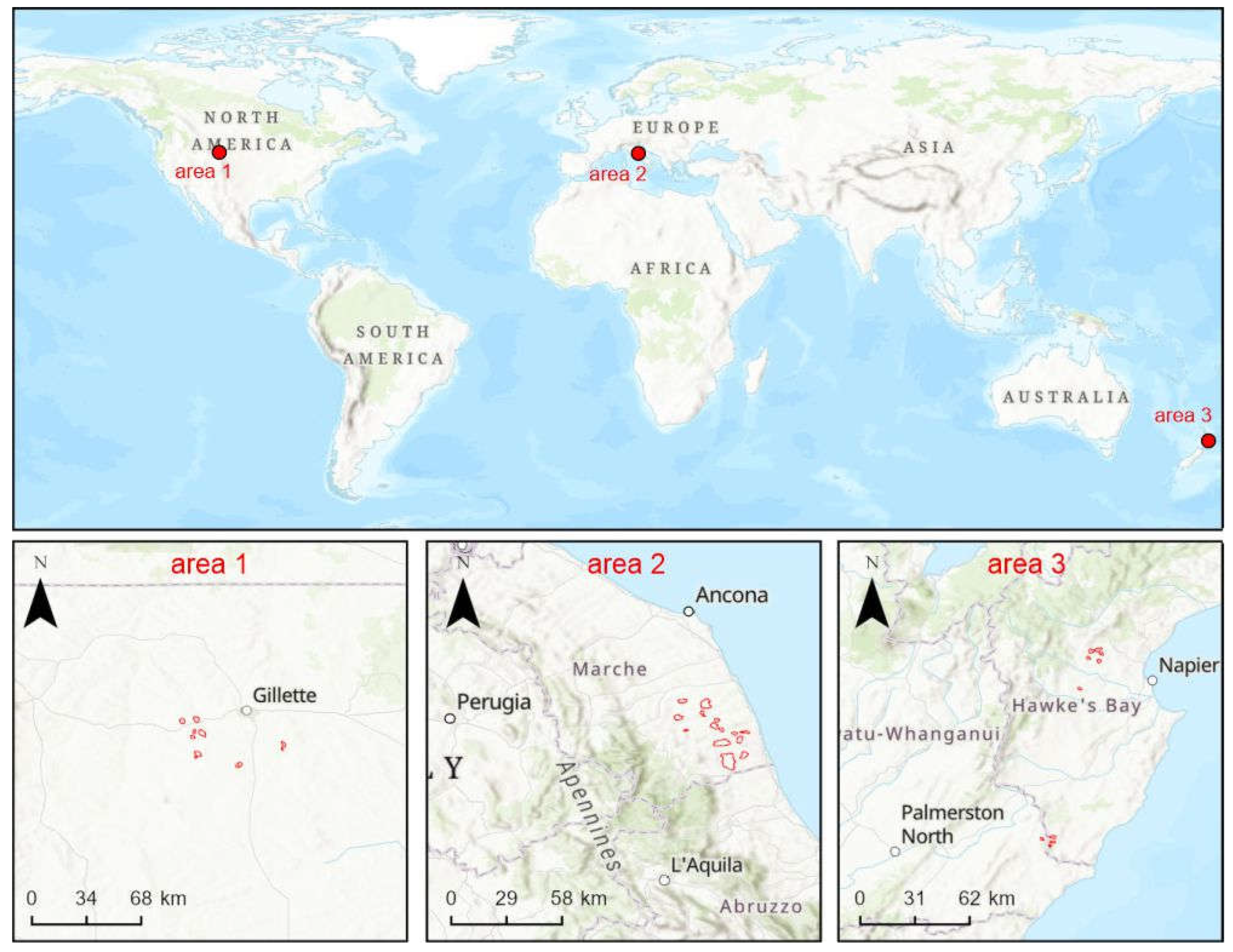
Figure 2.
(a) Lithological sketch of the Area 1 with the location of the basins investigated; (b) typical gullies visible from satellite image (top, source © Google Earth, 2025) and the ground (bottom). Modified from Ciccolini et al. 2024,.
Figure 2.
(a) Lithological sketch of the Area 1 with the location of the basins investigated; (b) typical gullies visible from satellite image (top, source © Google Earth, 2025) and the ground (bottom). Modified from Ciccolini et al. 2024,.
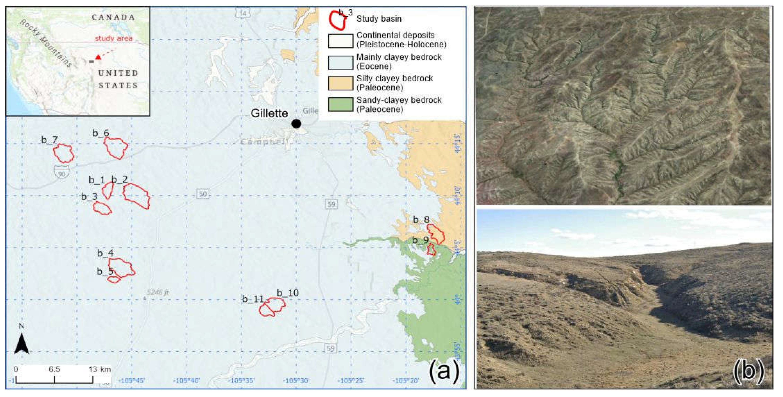
Figure 3.
(a) Lithological sketch of the Area 2 with the location of the basins investigated; (b) typical gullies visible from satellite image (top, source © Google Earth, 2025) and the ground (bottom). (Modified from Ciccolini et al. 2024).
Figure 3.
(a) Lithological sketch of the Area 2 with the location of the basins investigated; (b) typical gullies visible from satellite image (top, source © Google Earth, 2025) and the ground (bottom). (Modified from Ciccolini et al. 2024).
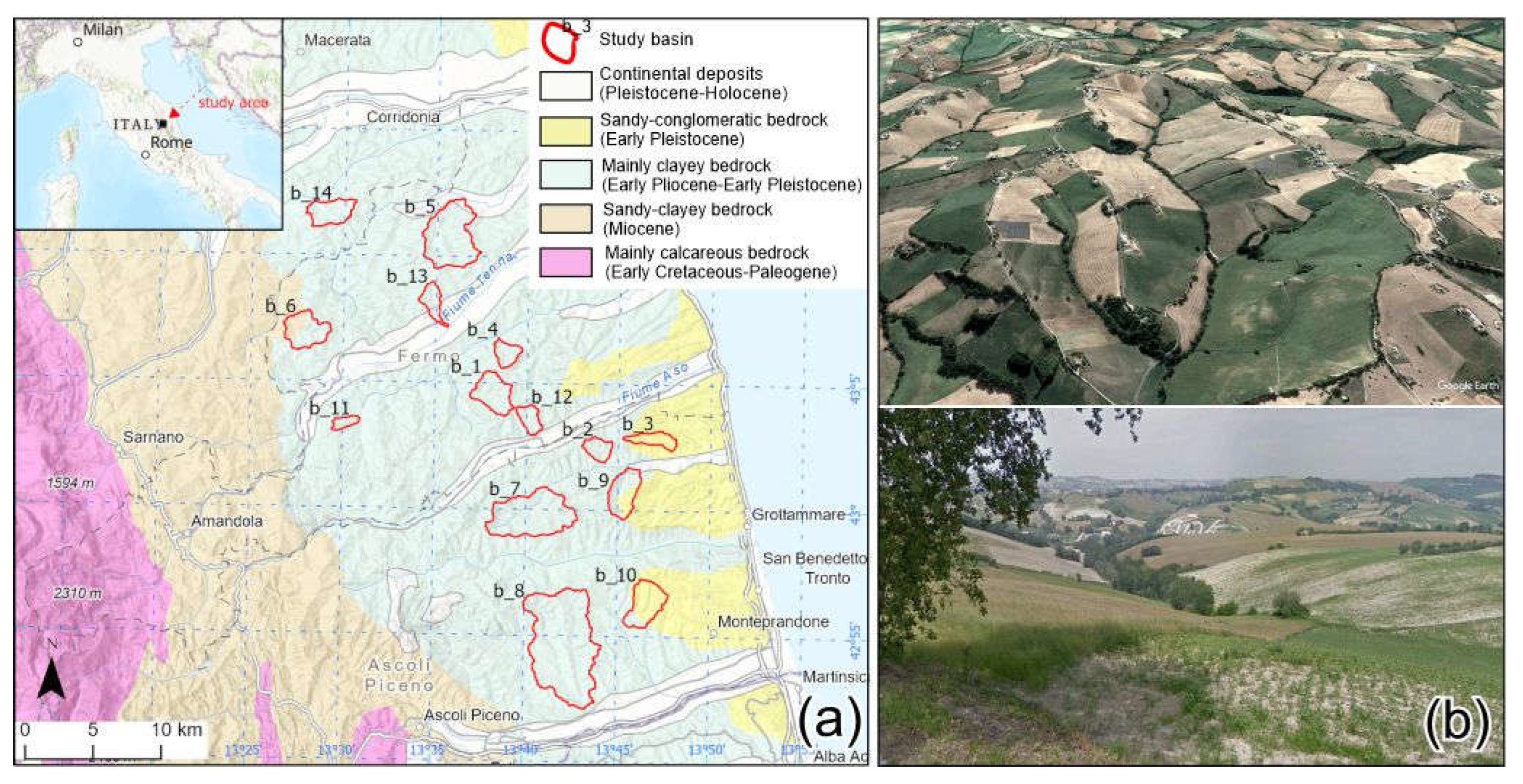
Figure 4.
Lithological sketch of the Area 3—(a) northern sector, (b) southern sector—with the location of the basins investigated; (c) typical gullies visible from satellite image (top, source © Google Earth, 2025) and the ground (bottom).
Figure 4.
Lithological sketch of the Area 3—(a) northern sector, (b) southern sector—with the location of the basins investigated; (c) typical gullies visible from satellite image (top, source © Google Earth, 2025) and the ground (bottom).
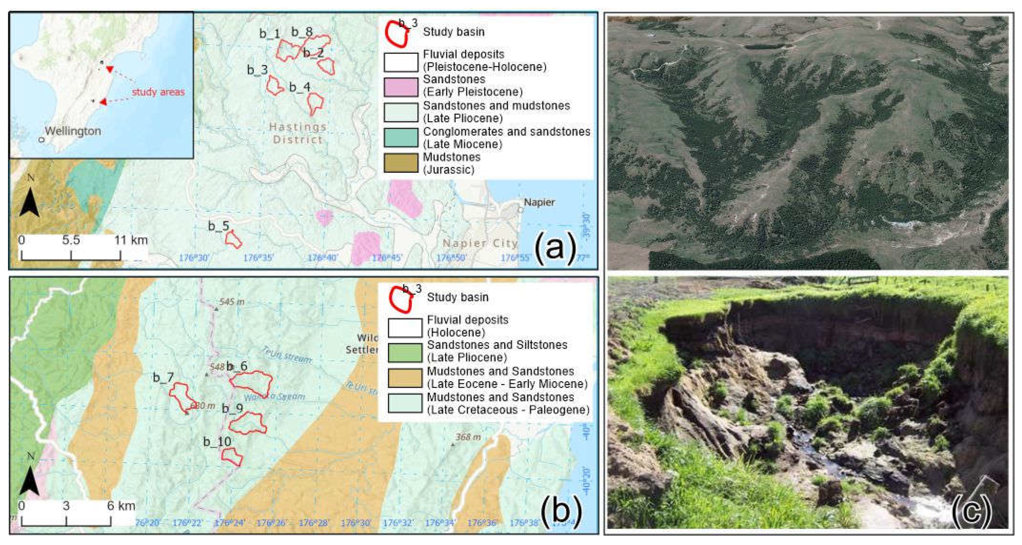
Figure 5.
a) Frequency distribution histogram showing the number of reaches (Nuz_i) divided per order; b) Example of basin with the points of intersection between the vector file of the hydrographic network and the vector file of the contour lines extracted from the DTM; c) Example of flow contribution curve (FCC) relating to the first three orders of hydrographic network.
Figure 5.
a) Frequency distribution histogram showing the number of reaches (Nuz_i) divided per order; b) Example of basin with the points of intersection between the vector file of the hydrographic network and the vector file of the contour lines extracted from the DTM; c) Example of flow contribution curve (FCC) relating to the first three orders of hydrographic network.
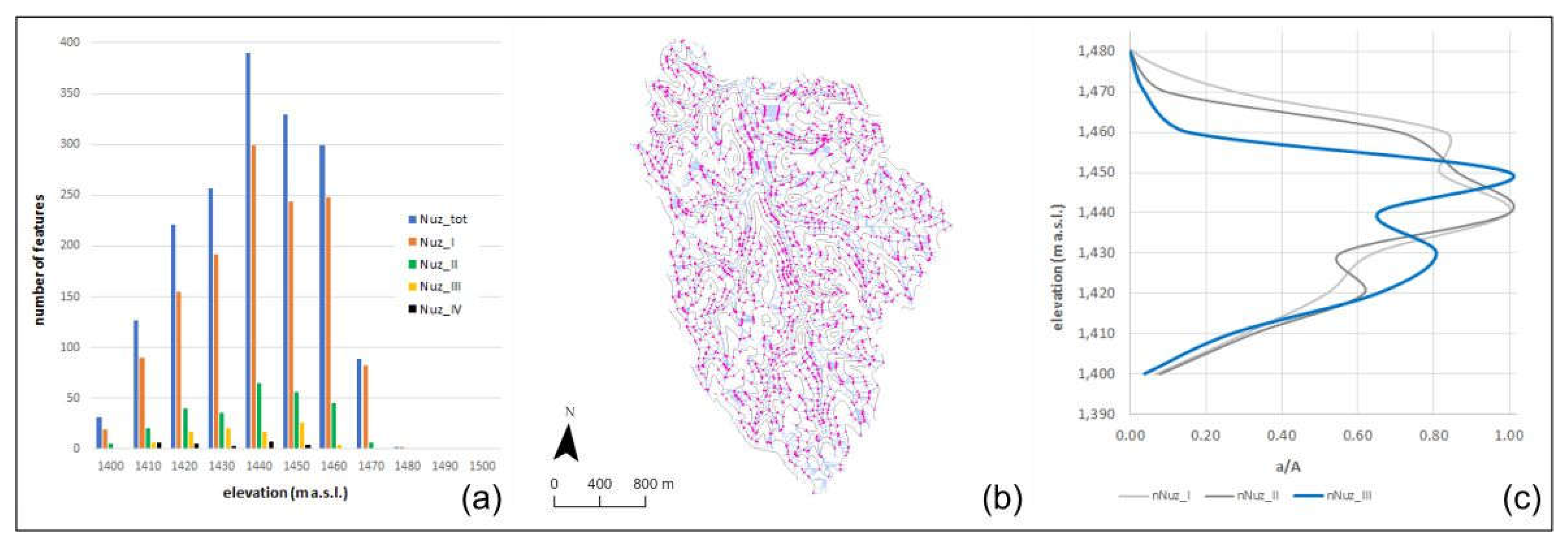
Figure 6.
Example of hypsometric curve with indication of value and location of the relating oblique inflection points (OIPs).
Figure 6.
Example of hypsometric curve with indication of value and location of the relating oblique inflection points (OIPs).
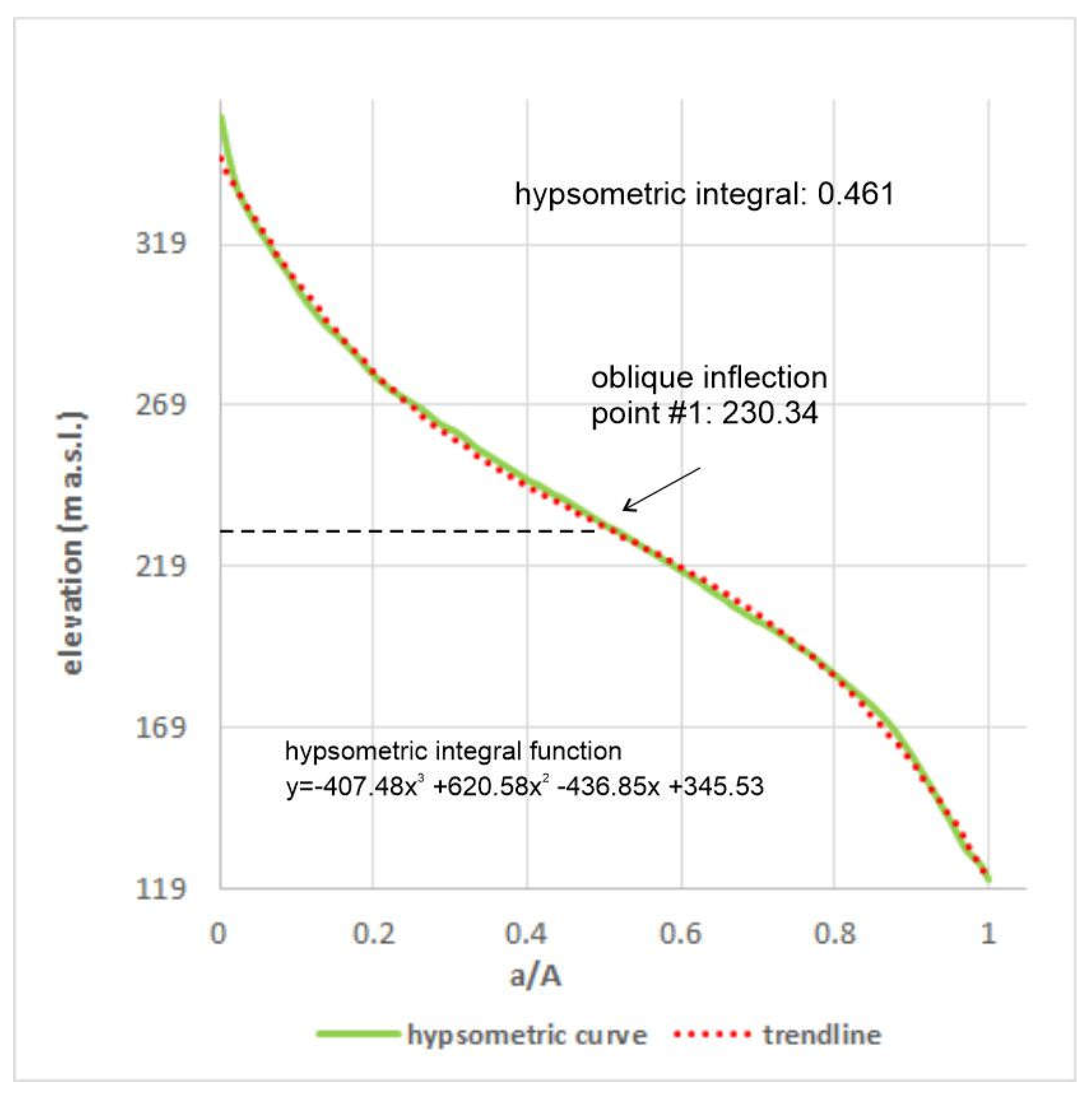
Figure 7.
Procedure for calculating the energy potential of running waters: a) DTM with 10m resolution; b) h/H raster; c) basin slope in radians; power P of the basin expressed in watts.
Figure 7.
Procedure for calculating the energy potential of running waters: a) DTM with 10m resolution; b) h/H raster; c) basin slope in radians; power P of the basin expressed in watts.
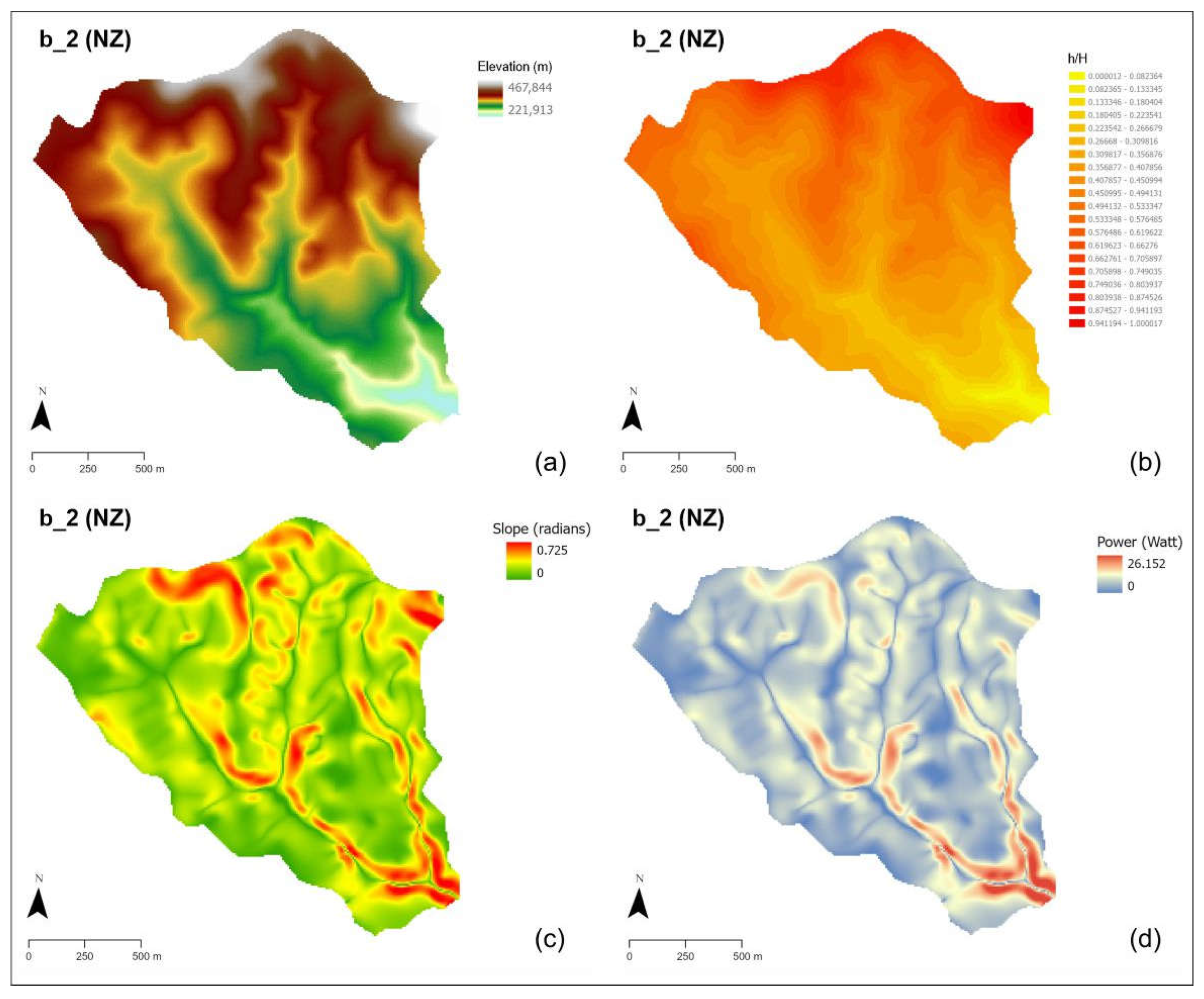
Figure 8.
Mapping of the gullies heads through the analysis of satellite images (source © Google Earth, 2025).
Figure 8.
Mapping of the gullies heads through the analysis of satellite images (source © Google Earth, 2025).
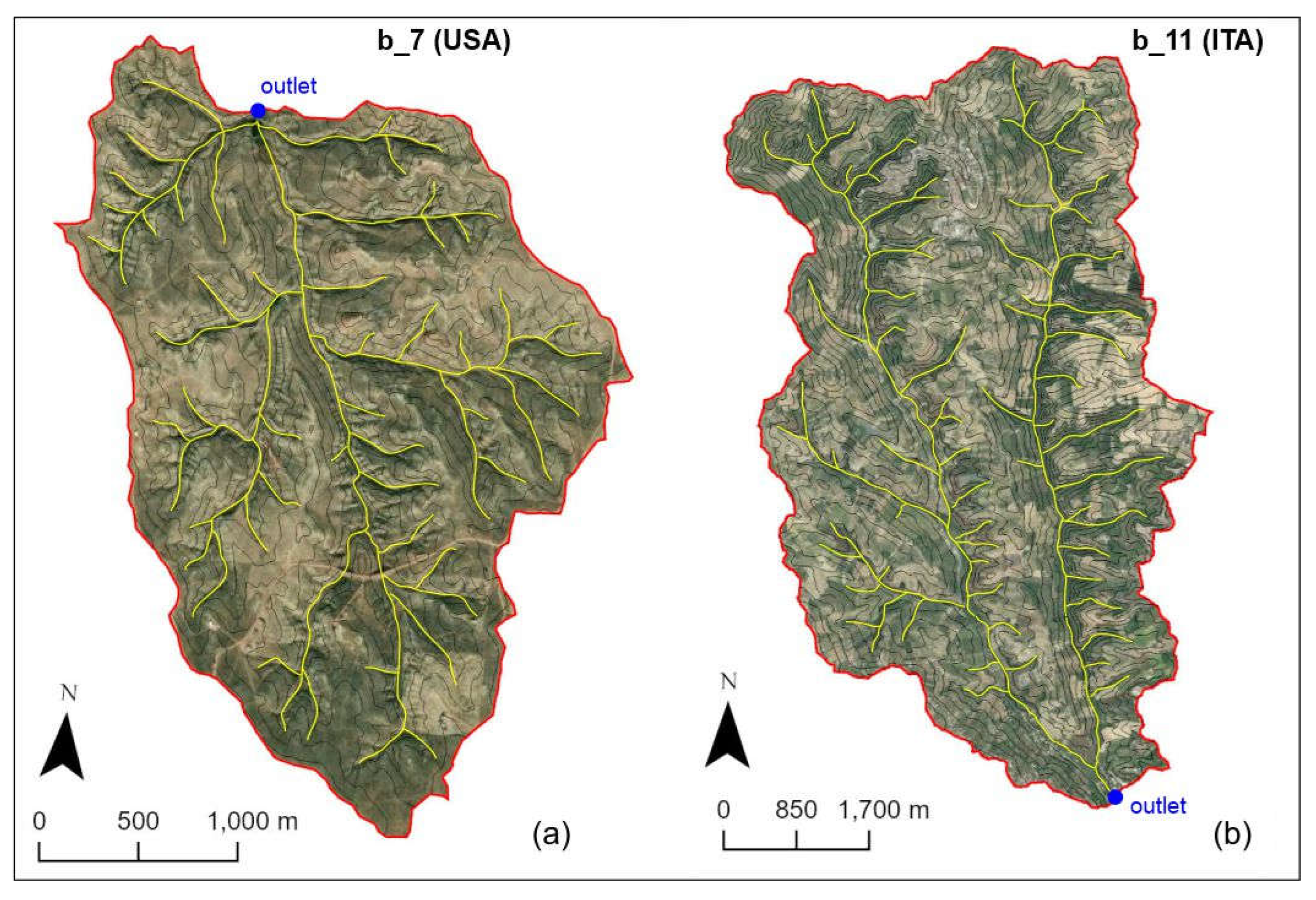
Figure 9.
Flow Contribution Curves (FCCs) of the first three order reaches and the corresponding hypsometric curves related to nine sample basins. Dashed lines of different colors indicate the mean heights of the gullies calculated with different methods; inside each figure the corresponding Oblique Inflection Point (OIP) is also reported.
Figure 9.
Flow Contribution Curves (FCCs) of the first three order reaches and the corresponding hypsometric curves related to nine sample basins. Dashed lines of different colors indicate the mean heights of the gullies calculated with different methods; inside each figure the corresponding Oblique Inflection Point (OIP) is also reported.
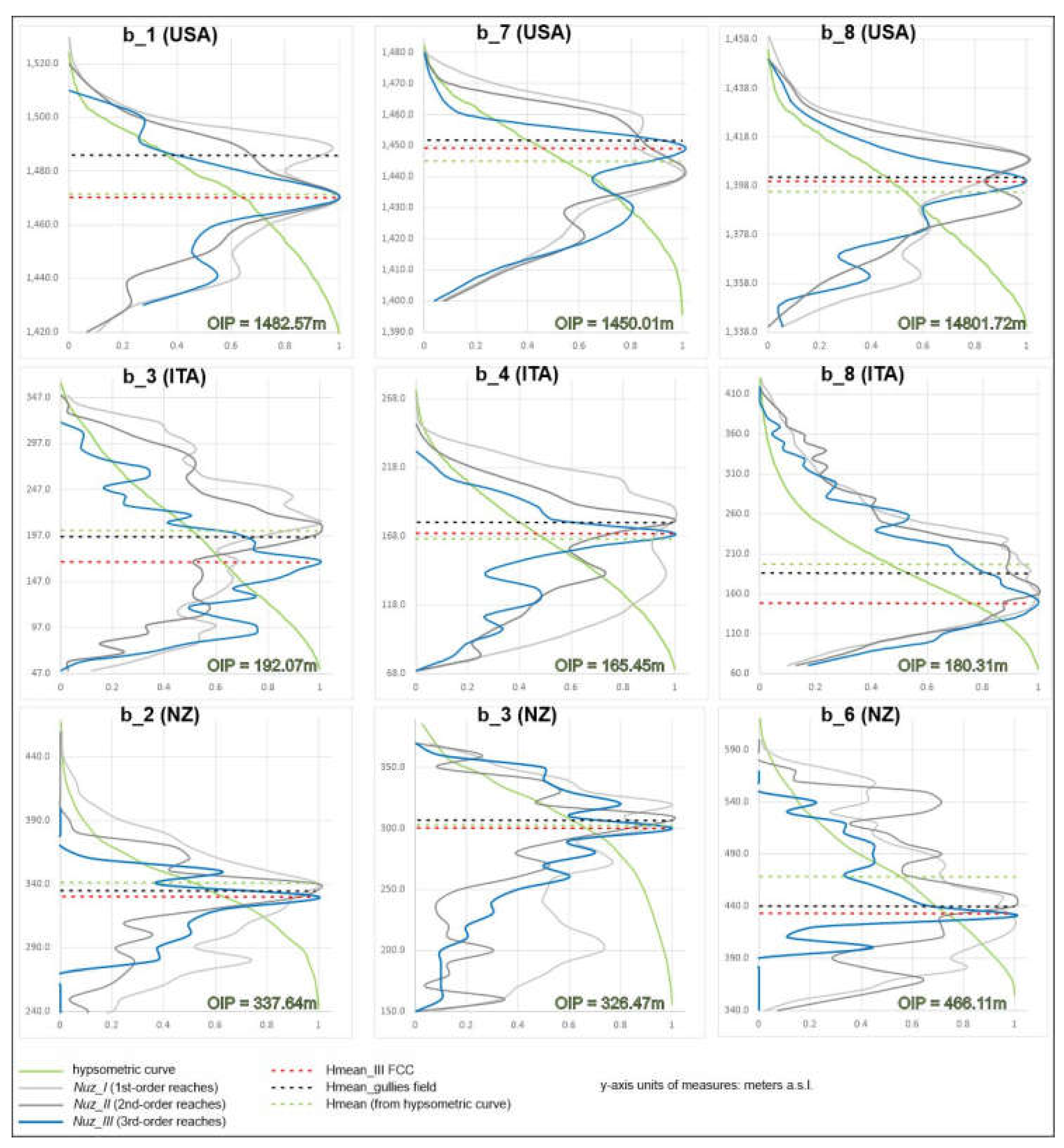
Figure 11.
Normal distribution a) and frequency distribution b) of the calculated Ei values.
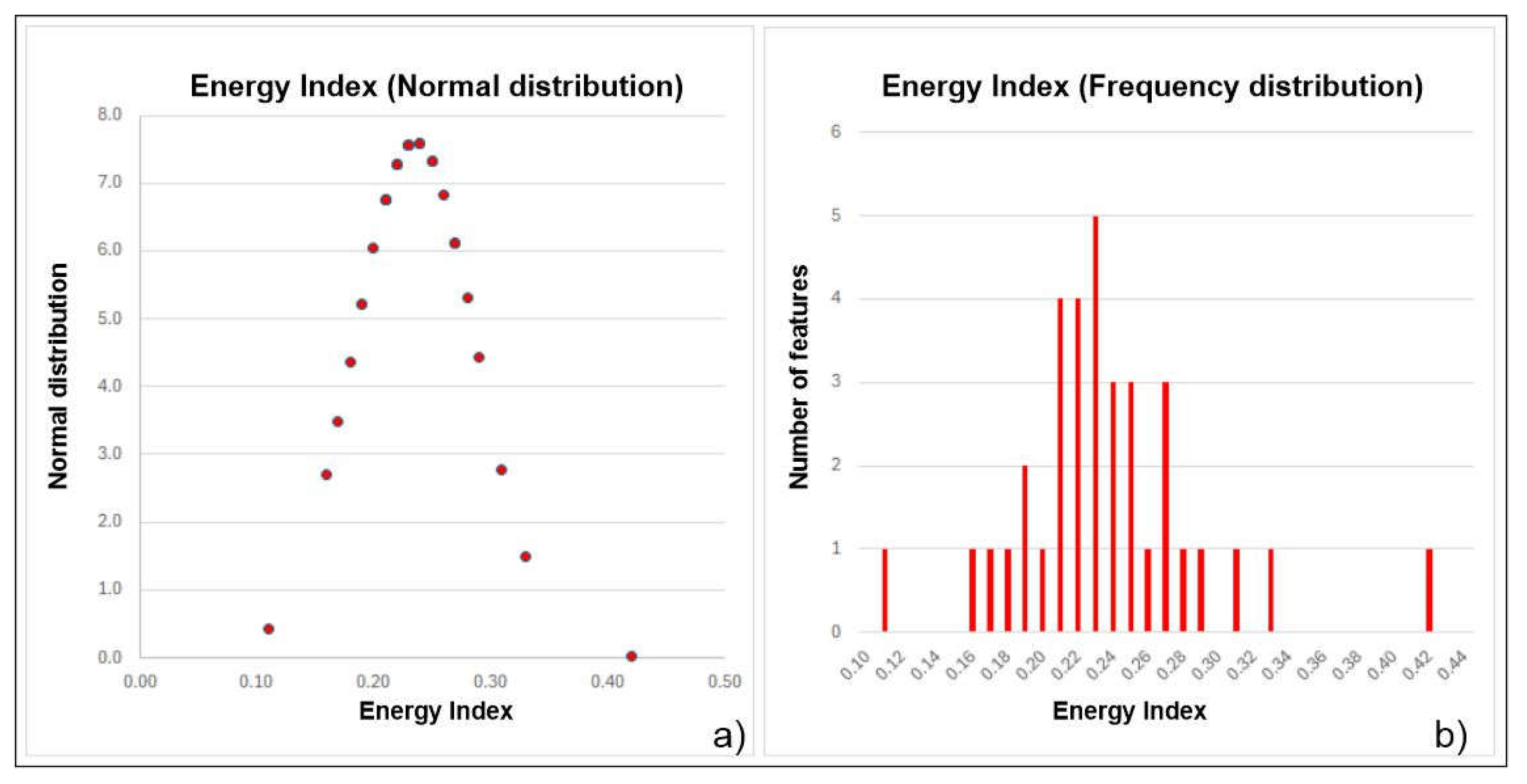
Figure 10.
a), c) and e) rasters of the water potential (expressed in watts) for three sample basins; b), d) and f) related satellite images (source © Google Earth, 2025); the yellow line indicates the contourline of the mean height of the basin.
Figure 10.
a), c) and e) rasters of the water potential (expressed in watts) for three sample basins; b), d) and f) related satellite images (source © Google Earth, 2025); the yellow line indicates the contourline of the mean height of the basin.
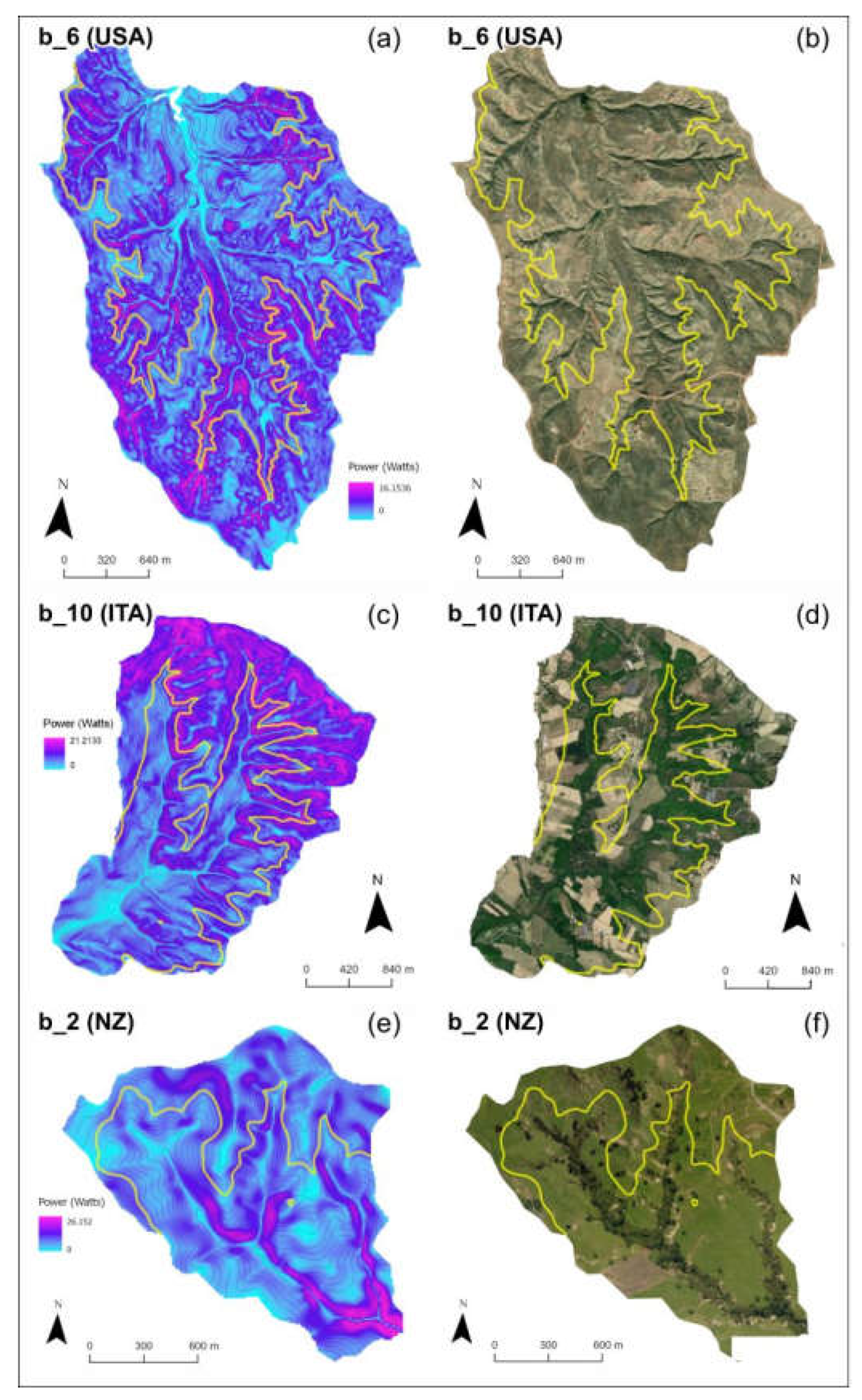
Figure 12.
Comparison between Energy Index and some basic morphometric parameters: a) hypsometric integral; b) basin area; c) mean height; d) average slope; e) circularity ratio.
Figure 12.
Comparison between Energy Index and some basic morphometric parameters: a) hypsometric integral; b) basin area; c) mean height; d) average slope; e) circularity ratio.
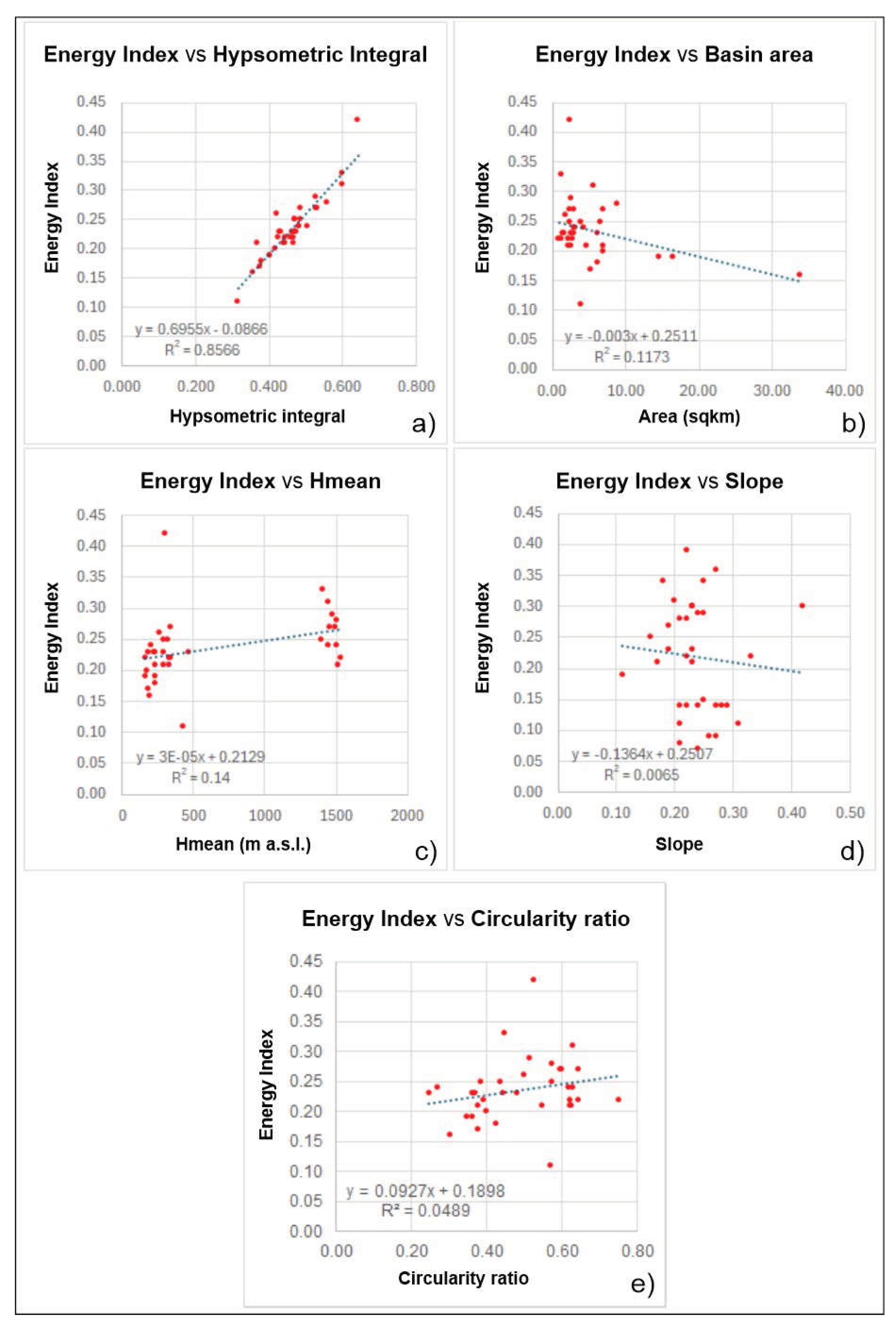

Table 1.
Summary table with all the processing results described in the text.
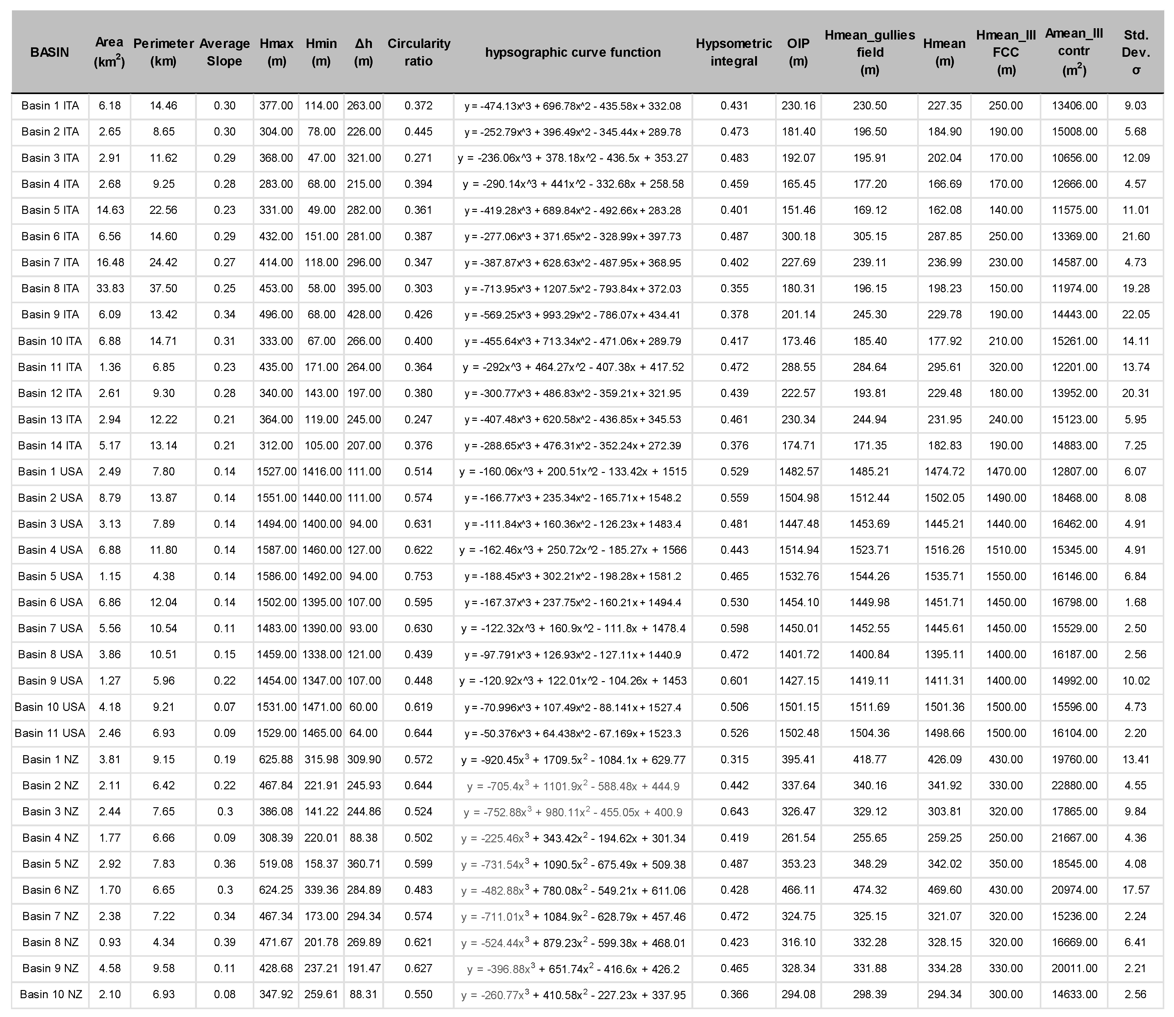
Table 2.
Şen’s “Energy Index” (Ei) calculated for all the basins analyzed.
Disclaimer/Publisher’s Note: The statements, opinions and data contained in all publications are solely those of the individual author(s) and contributor(s) and not of MDPI and/or the editor(s). MDPI and/or the editor(s) disclaim responsibility for any injury to people or property resulting from any ideas, methods, instructions or products referred to in the content. |
© 2026 by the authors. Licensee MDPI, Basel, Switzerland. This article is an open access article distributed under the terms and conditions of the Creative Commons Attribution (CC BY) license (http://creativecommons.org/licenses/by/4.0/).
Copyright: This open access article is published under a Creative Commons CC BY 4.0 license, which permit the free download, distribution, and reuse, provided that the author and preprint are cited in any reuse.


