
Submitted:
07 August 2026
Posted:
07 August 2026
Read the latest preprint version here
Abstract
FEFLOW is used to provide a design stage analysis of seepage flow through a tailings storage facility constructed by on-dam cycloning, including phreatic surface level, drain flows, and water balance. Significant differences between simulation results and measurements of dam crest piezometer data and foundation flows highlight possible structural issues with hydraulic conductivity gradient of the tailings beaches, hydraulic conductivity of the downstream shells, and internal erosion. Partial saturation of tailings beach material is accounted for by solving Richards’ transient flow equation throughout facility staged construction, using MATLAB seepage analysis of an idealized 1D staged construction processes as an initial benchmark for setting FEFLOW time stepping and mesh size parameters. Seepage analysis of an idealized 2D staged construction process is used to clarify the importance of solving Richards’ transient flow equation for accurate tailings dam phreatic surface location.
Keywords:
tailings dams
; staged construction
; transient seepage analysis
; Richards’ equation
1. Introduction
On-dam cycloning is a common method of constructing tailings storage facilities (TSFs) whereby total tailings and/or cyclone overflow spigotted from the facility periphery settles out across one or more tailings beaches with decreasing grain size towards the tailings pond. The Kareerand TSF in Matlosana, South Africa is an example of a TSF constructed by this method [12]. To correctly assess slope stability of TSF dams, including those constructed by on-dam cycloning, it is of critical importance to analyze the seepage of water through TSFs [15]. For example, after breach of the Jagersfontein TSF in 2022, an investigation panel identified several factors contributing to failure including high phreatic surface level caused by the reprocessed tailings deposition method and absence of a decant facility [24]. This fact points to the importance of using seepage analysis during TSF design phase to conservatively predict the effect of phreatic surface level and pore water pressure on dam stability, and of using seepage analysis to explain deviations of as-built phreatic conditions from design phase predictions.
Figure 1 shows an example of a TSF design layout with 2D cross sectional geometry and 3D geometry based on the design of a currently operational TSF constructed by on-dam cycloning. The TSF is a cross valley copper tailings impoundment with two tailings dams, West and East, providing containment. The layout in Figure 1 is a bird’s eye view of the TSF whose 3D geometry is constrained by the valley topography. The TSF is reactivated, in that the TSF was inactive for 15 years 1997-2011 before being used for another 14 years 2012-2025. Each dam is constructed on top of a 30[m] thick sand and gravel foundation with clay lenses, and contains a foundation underdrain, starter dam, cycloned sand downstream shell, tailings beach, and tailings slimes. The top of the foundation is assumed to coincide with the local groundwater table at the start of TSF construction, at elevation 800[m], except where 2.5[m] thick underdrains have been constructed with excavation of foundation material. The original TSF, used for 25 years before 1997, was built up to a dam crest elevation of 850[m] by centreline construction, followed by upstream construction until 1997. By the end of 2025, the reactivated TSF was built up to a dam crest elevation of 983[m] and tailings pond elevation of 973[m] by centreline construction, starting from a dam crest elevation of 913[m] at the beginning of 2012. Sloping sidewalls of the valley create a longitudinal dam cross section that is 750[m] wide at elevation 973[m] and 250[m] wide at the bottom of the TSF foundation at elevation 770[m]. West and East Dam tailings beaches of the TSF are assumed to have been maintained at widths of 525[m] and 560[m] throughout construction, although Figure 1 does not delineate boundaries of the beaches prior to 1997.
Important factors determining the location of phreatic surface level through a TSF dam include the length of the tailings beach between the dam crest and tailings pond, the gradient of hydraulic conductivity across the tailings beach, drainage, and the rate of TSF construction, which in the case of construction by on-dam cycloning controls the spigotting water recharge rate. An appreciation for the qualitative influence of beach hydraulic conductivity gradient and spigotting recharge rate on dam phreatic surface level can be obtained using the Dupuit-Forchheimer approximation for seepage flow, in which seepage is assumed to be horizontal, and the phreatic surface height along the length of the dam satisfies the differential equation:
where is the distance to the edge of the tailings pond, is the saturated horizontal hydraulic conductivity of dam material, and is the spigotting recharge rate [5]. Solutions to the Dupuit-Forchheimer equation subject to the boundary conditions [m] and [m] are shown in Figure 2 for hydraulic conductivities and recharge rates of: (a)[m/s] and 0[m/year], (b) [m/s] and 2.5[m/year], (c) [m/s] and 0[m/year], and (d) [m/s] and 2.5[m/year]. A difference in concavity of the phreatic surface is evident between uniform and exponentially increasing hydraulic conductivity cases (a) and (c) where recharge rate is 0, and increase in phreatic surface occurring with non-zero recharge rate is evident in cases (b) and (d). The exponentially increasing hydraulic conductivity is selected so that and [1]. Note that the phreatic surface level computed by Dupuit-Forchheimer approximation for the case of exponentially increasing hydraulic conductivity and non-zero recharge is not physically realistic, in that the phreatic surface rises above the level of the tailings pond at 100m as the distance to the tailings pond increases from 0m, so more accurate description of seepage through saturated tailings beach material deposited near the pond edge is required to obtain physically meaningful results.
Figure 2 suggests accurate description of how tailings beach hydraulic conductivity and recharge rate influence seepage flow is necessary during the TSF design process for accurately approximating phreatic surface level in slope stability factor of safety computations. In theory, this requires solution of the Richards’ transient flow (RTF) equation through partially saturated regions of the TSF such as the tailings beaches, coupled to solution of solid mechanics equations describing tailings dam structural deformation. However, while it is generally accepted that analysis of groundwater contamination beneath a tailings dam requires solution of Richards’ transient flow (RTF) equation, it has been stated that for the purpose of slope stability analysis, solution of saturated flow equations often provides a conservative estimate of phreatic surface level within tailings dams [26]. This statement is reinforced by seepage analysis methods employed by investigators of high profile tailings dam failures such as the Fundão tailings dam, whose analysis involved solution of the saturated transient flow (STF) equation using the commercial finite element solftware FEFLOW [18]. Moreover, slope stability analyses of tailings dams throughout staged construction often use empirical phreatic surfaces specified by piezometer data rather than numerically simulated phreatic surfaces to ensure realistic results [19]. Perhaps for these reasons, while previous work has used solution of the RTF equation to analyze slope stability of a hydropower embankment dam under changes in reservoir level, examples of solving the RTF equation to analyze seepage flow throughout staged construction of tailings dams are difficult to find [27]. Nevertheless, it remains possible that at the TSF design stage, solution of the RTF equation offers some practical engineering advantage in seepage analysis accuracy over solution of saturated flow equations, particularly for facilities that are reactivated and/or contain partially saturated tailings beaches as a result of dam construction by on-dam cycloning with hydraulic segregation of tailings. For this reason, the purpose of this article is to apply the FEFLOW RTF solver, previously applied to simulate tailings dam groundwater contamination, to provide a design stage seepage analysis of a TSF that is both reactivated and constructed in stages by on-dam cycloning, and to compare the results of this analysis with as-built TSF measurements as an initial diagnosis of any structural problems [7].
The outline of the article is as follows. Chapter 2 describes MATLAB finite difference solution of the 1D RTF equation for a 1D tailings beach staged construction process for benchmarking FEFLOW simulation of staged construction, and discusses selection of TSF staged construction simulation input parameters for FEFLOW. Chapter 3 compares FEFLOW solutions of the 2D RTF and STF equations for seepage flow throughout an idealized 2D staged construction process to justify importance of solving the RTF equations, and provides 2D FEFLOW simulation results for seepage flow through a TSF with two tailings dams constructed in stages by on-dam cycloning. These results include phreatic surface level, drain flows, water balance, with comparsion to reported measurements of dam crest piezometer readings and total foundation flows. Chapter 4 summarizes the article results.
2. Materials and Methods
Transient Flow Equations
The STF equation is:
where is pore water pressure head, is the saturated material hydraulic conductivity tensor, is material specific storage, and is a fluid source/sink term. Typical parameter values assigned to different tailings dam construction materials are shown in Table 1 [5,21]. In this table, and are the saturated horizontal and vertical material hydraulic conductivities.
The RTF equation describing unsaturated transient pore water flow is:
where is pressure head, is elevation head, is the unsaturated hydraulic conductivity tensor, is the volumetric water content, and is a fluid source/sink term. The Van Genuchten equation:
expresses the volumetric water content in terms of the residual volumetric water content , saturated volumetric water content (i.e. unsaturated-flow porosity) , air entry , and pore size distribution , with taking a value between 0 and 1. The Mualem-Van Genuchten equation:
expresses the unsaturated hydraulic conductivity tensor in terms of the saturated hydraulic conductivity tensor and effective saturation:
1D Staged Construction Benchmark
Although FEFLOW provides a well established Richards’ equation solver, numerical accuracy of the solver output still depends on problem mesh size and time step, and should be verified against analytic solution if at all possible [23]. More specifically, even when the mixed head-saturation formulation of Richards’ equation is used, fluid mass balance errors can persist with poor convergence of the FEFLOW nonlinear iterative (e.g. Picard) solution for saturation and pressure head at each time step, particularly when the solution involves propagation of a wetting front with a sharp drop off in hydraulic conductivity from saturated to unsaturated regions [4]. For this reason, a 1D MATLAB RTF finite difference solver, verified against 1D analytic solutions for Gardner evaporative drying and Philip short-time infiltration with Van Genuchten unsaturated flow material parameters, has been used to benchmark FEFLOW simulation of seepage flow through a column of tailings beach material for an idealized 1D staged construction process [6,11,14]. Writing this solver allows for detailed examination of how time stepping and spatial discretization parameters influence Picard solver stability in a way that is not currently possible through any commercial FEFLOW user interface, and for quicker computation of 1D RTF equation solutions on a true 1D grid.
The 1D staged construction process occurs with annual 5m tailings beach lifts for 20 years on top of a drain at elevation 0m. The 1D RTF equation is solved in mixed head-saturation form by finite differences using the implicit Euler method in MATLAB. Explicitly, the nonlinear equation to be solved at each time step by Picard iteration can be written as:
where indexes space and indexes time. Between construction lifts, 0 hydraulic head and 0 flow boundary conditions are imposed at elevation 0m and the 1D column surface elevation. Total hydraulic head within newly added saturated material is initialized to be constant at the column’s new surface elevation except within a boundary layer of thickness [cm] between newly deposited saturated material and previously deposited unsaturated material at elevation , where a pressure head gradient:
is defined to improve stability of the finite difference Picard nonlinear solver [9]. The finite difference grid spacing is [cm], and the time step is adaptively increased from 0.1[s] immediately after new construction to a maximum value of 1.5 days by factors of 2 whenever the number of Picard iterations required for pressure head convergence within [m] is less than 14.
Figure 3 shows pressure head and water content profiles for a 1D staged construction process after stages 14 and 20, computed by finite difference solution of the 1D RTF equation for a tailings beach material with [m/s],
[1/m], , , and . This solution suggests that away from the top and bottom of the column of material, water content remains at a constant value as construction proceeds beyond the first 10 stages of construction. Similar water content profiles are observed when saturated vertical hydraulic conductivity is varied between values [m/s] and [m/s], as indicated by Figure 4-left where at stage 20 is plotted against . Figure 4-right shows a plot of annual average drain flow for stage 20 against . For all conductivity values:
where is the rate of construction 5[m/year], and an upper bound for drain flow as is increased beyond [m/s] is [L/s]. For the plotted range of saturated vertical hydraulic conductivities, the drain flow at [m] is approximately constant throughout stage 20 at the value , and approximately linear dependence of follows from solving the equation:
and using the fact that the Mualem-Van Genuchten hydraulic conductivity function satisfies:
for.
Using MATLAB finite difference simulation results as a benchmark, FEFLOW simulations of seepage flow during 1D staged construction were conducted using a 2D geometry of final height 100[m] and width 50[m] with no lateral variation of material parameters and equilateral triangular meshes of side length 1.44[m], .072[m], and 0.36[m]. Simulation results are anticipated to depend on finite difference grid spacing or finite element mesh size when this distance is greater than approximately 20 percent of the wetting front thickness length scale . As shown in Figure 5 for , the 0.36[m] element side length FEFLOW solution of the 2D RTF equation for water content profile showed good agreement with the 0.1[m] grid spaced MATLAB finite difference solution of the 1D RTF equation for water content profile after stage 20. Mean absolute error between these water content profile was calculated to be . Similar agreement between MATLAB and FEFLOW computed water content profiles was found for a range of saturated vertical hydraulic conductivities [m/s], with a maximum difference in values of less than 0.01 across this range.
2D TSF Staged Construction Input Parameters
Initial Conditions
To specify phreatic conditions within the TSF existing at the time of reactivation, the effect of 15 years of TSF inactivity on phreatic conditions is simulated using the FEFLOW RTF solver starting from a conservative 1997 condition of complete water saturation of the TSF for which the pressure head of all materials in the TSF above elevation 0[m] is initialized to 0[m] and the hydraulic head of the underdrains and foundation is initialized to 0[m]. Seepage collection ponds with surface elevation 0m are present downstream of both West and East Dams, whereby 0[m] hydraulic head boundary conditions are assigned to the left edges of the West Dam underdrain and foundation and right edges of the East Dam underdrain and foundation, and no flow boundary conditions are assigned elsewhere under the assumption no tailings pond is present during deactivation. Depth dependent void ratio and hydraulic conductivity of tailings slimes are assigned based on 1D self weight consolidation simulation, and depth dependent tailings beach hydraulic conductivities are assumed to decay exponentially with distance from the dam crest to tailings slimes values at the material boundaries. TSF material parameters used to simulate phreatic conditions within the TSF during 15 years of inactivity are shown in Table 1 and Table 2.
Staged Construction Boundary Conditions
After reactivation, the TSF impoundment is increased in height by 5[m] each year. This height increase is modeled in FEFLOW by activating a new 5[m] layer of the TSF geometry each year. Within each newly activated layer, the hydraulic head at each location at time of deposition is initialized to a constant equal to the height of TSF at that location, under the assumption consolidation of newly deposited material occurs immediately, except at the interface between newly and previously deposited material where pressure heads are matched with a gradient smoothing function. No flow boundary conditions are specified on all TSF boundaries except at the location of the tailings pond where a constant hydraulic head equal to the height of the TSF is imposed, at the left edges of the West Dam underdrain and foundation where 0m hydraulic head boundary conditions are imposed, and at the right edges of the East Dam underdrain and foundation where 0[m] hydraulic head boundary conditions are imposed. Using the FEFLOW Python Interface Manager (IFM), depth dependent void ratio and hydraulic conductivity of tailings slimes are updated with activation of each new construction stage based on 1D self weight consolidation simulation, and depth dependent tailings beach hydraulic conductivities are updated with each new construction stage to decay exponentially with dam crest distance from dam crest values to tailings slimes values. The transient effect of undrained construction loading on TSF pore water pressure is not considered in the analysis, whose primary objectives are to compute phreatic surface level, underdrain flows, and TSF water balance.
Consolidation Water
While undrained construction loading occurs suddenly without change in underlying material porosity, consolidation is the gradual process by which the porosity of material decreases in delayed drainage response to construction loading. Authors of the Fundão investigative report used 1D FSConsol simulation of tailings sands and slimes consolidation to update the porosity and consolidation water production of tailings dam structural elements at each time step of the FEFLOW STF solver with an external program tracking changes in effective stress within the dam. Here, to avoid numerical instability of the FEFLOW RTF solver, a different 1D approximation of tailings slimes consolidation is used, whereby 1D self weight consolidation of tailings slimes is simulated by solving the 1D finite strain consolidation equation by finite differences, and the resulting time dependent porosity profile is used to adjust the porosity of tailings slimes elements each time a new tailings lift occurs [20,22]. So that fluid mass balance is preserved, a consolidation water source is introduced for each tailings slimes element with a water production rate specified by the annual change in element porosity. This approximation accounts for consolidaton water production in TSF transient seepage analysis without directly coupling RTF and consolidation equation solutions. However, it should be noted that because the geometry of newly activated layers is fixed in FEFLOW, this approximation does not account for consolidation settlement of slimes, and for this reason annual adjustments to structural element porosity are based on linear interpolation of void rato vs height curves for the end of each year 2012-2024 from end of 2011 and end of 2025 curves obtained by simulation.
1D consolidation equations expressing void ratio and saturated vertical hydraulic conductivity in terms of vertical effective stress:
are used with copper tailings slimes constants to simulate self weight consolidation of tailings slimes [2]. A maximum void ratio of 1.46 is assigned to slimes at the surface of the TSF. Figure 6 shows 1D simulation results for (a) tailings slimes impoundment total height across the history of TSF staged construction starting from 1973, and end of 2025 vertical profiles for tailings slimes saturated vertical hydraulic conductivity, void ratio, and excess pore pressure. 1D consolidation water flux out of the top and bottom of the impoundment is computed to be 1.6[m/year] and less than 0.1[m/year] at the end of 2025.
3. Results
2D RTF/STF Seepage Analysis Comparison
To justify the importance of solving the RTF equation to 2D tailings dam seepage analysis, a comparison of 2D STF and RTF seepage flow solutions for a 2D tailings beach staged construction process is provided. The beach embankment is constructed over 14 years in annual 5m lifts to a final dimension of 70m high by 400m wide.
Steady State
Figure 7-top shows (a) RTF quasi-steady state and (b) STF steady state phreatic surface levels after the final construction stage of a 70m high by 400m wide tailings beach embankment, computed using FEFLOW transient solvers to obtain stable convergence of the solution to steady state. In both cases, the upstream boundary condition is a constant hydraulic head of 70m, and the downstream boundary condition is a constant hydraulic head of 0m along a 100m long drain, with all other boundary conditions on the rectangular domain being Neumann 0 flow. Saturated horizontal hydraulic conductivity of tailings beach material increases exponentially from 1e-7[m/s] to 1e-5[m/s] as distance from the upstream boundary increases from 0[m] to 300[m], and the vertical to horizontal saturated hydraulic conductivity ratio is 0.1. Material specific storage is 1e-4[1/m], and for RTF solution, Van Genuchten parameters , , and are selected. The FEFLOW mesh used for solving the RTF and STF equations has 9483 nodes and 18576 triangular elements with side lengths between 1.2[m] and 2.5[m] and a typical side length of 1.75[m]. Refinement of this mesh was not observed to alter the RTF phreatic surface level for .
The computed STF steady state solution pressure head is roughly approximated by the analytic expression:
which solves the STF steady state equation on the rectangular domain with a non-zero Dirichlet boundary condition along the underdrain. Semi-analytic solution for the RTF steady state pressure head is obtained for by noting that in this limit:
whereby the expansion:
for the RTF steady state pressure head implies:
upon substitution in the RTF equation. Solving this differential equation with a MATLAB 2D finite difference solver gives the plot of shown in Figure 7-bottom, providing evidence that the difference between RTF and STF steady state phreatic surfaces observable in Figure 7-top is reasonable.
Figure 8 shows plots of total water content vs time and average pressure head vs time for FEFLOW quasi-steady and steady state solutions of the RTF and STF equations initiated from STF steady state and RTF quasi-steady state solutions. The STF solution fit (d) shows exponential decay of average pressure head to a constant value with time constant 14.28[days], in approximate agreement with the longest decay time constant of 13.70[days] computed in MATLAB by solving a Helmholtz linear eigenvalue problem with mixed homogeneous Dirichlet and Neumann boundary conditions on the solution domain. The RTF solution fit (c) shows approximately exponential decay of total water content to a constant value over the first 20 years of simulation, with fitting time constant 8.69[years], before continuing to increase at a rate in disagreement with exponential decay. Deviation of RTF transient decay time constants from STF transient decay time constants is not explained by analyzing transient corrections to the STF steady state solution of order , since these transients decay with STF decay time constants. A possible explanation for disagreement of long term RTF transient decay with exponential decay is that for Van Genuchten/Mualem material parameters, the RTF long term description of the dry capillary fringe water content decreases to 0 in time by a power law in rather than an exponential, so exponential fitting is not generally valid and cannot be assumed to return the same transient decay time constant for all initial pressure head conditions.
As a practical rule of thumb, and as evidenced by 1D staged construction benchmarking, a finite element mesh element size of at most 1 is recommended when solving the RTF equation to accurately resolve capillary wetting of unsaturated material. However, to achieve TSF staged construction simulation times on the order of hours on a Microsoft Azure FEFLOW licensed virtual machine with 8vCPUs and 64GB of RAM, it is necessary to use a significantly larger mesh size. Table 3 shows the effect of refining triangular element side length from 1.44[m] to 0.36[m] on phreatic surface level, drain flow, and water content. Differences in phreatic surface level and water content are tabulated in terms of mean absolute error and max absolute error with respect to the element size 0.36[m] simulation result. In all cases, the RTF quasi-steady state drain flow is [day], approximately half of the STF steady state drain flow []. When the value of is increased to 1, 2, and 4, inspection of the RTF quasi-steady state solution suggests it is necessary that the mesh size be at most 3.5 to avoid occurrence of spurious
Staged Construction
Figure 9-top shows the end of construction RTF transient phreatic surface level and saturation computed throughout 14 stages of 5[m] height increase each year. Figure 9-bottom shows the final stage quasi-steady state phreatic surface level and saturation. In both cases, complete saturation is indicated by red coloration, near residual saturation is indicated by violet/blue coloration, and transition between complete and residual saturation is indicated by green coloration. Close inspection of solutions (a) and (c) in the FEFLOW GUI indicates that the RTF transient phreatic surface is nearly identical to the RTF steady state phreatic surface. However, it is also clear from the figure that the water content of unsaturated material within the tailings beach, equal to half the saturation for material porosity 0.5, is different between RTF staged construction and quasi-steady state solutions.
Based on 1D MATLAB finite difference simulations the initial FEFLOW simulation time step is selected as 0.1[s] with maximum adaptive time step increase of up to a maximum time step of 1.5[days]. With these settings, and , the FEFLOW solver shows no indication of Picard iteration instability, meaning the residual rate balance:
remains less than the FEFLOW default specified error tolerance of 0.0001[day]. However, when the Van Genuchten parameter is decreased from 2 to 1.5, FEFLOW indicates Picard iteration instability during stage 11, due to increased water retention in unsaturated material increasing the residual rate balance. If the parameter is not too close to 1, this problem can be solved by increasing the FEFLOW default number of Picard iterations, as is the case for if the number of iterations is increased from 12 to 30.
2D TSF Staged Construction Seepage Analysis
Quasi-Steady State Phreatic Surface Level and Water Balance
As a point of reference for staged construction simulation results, the end of 2025 TSF quasi-steady state RTF phreatic surface level and drain flows have been computed using a 10 year approach to steady state. Figure 10 (a) shows the FEFLOW computed RTF phreatic surface level, using a mesh with 109205 nodes and 217044 triangular elements. The pond inflow rate is 0.65 [day], and the total drain/foundation outflow rate is 2.42[day], indicating that after 10 years of approach to steady state and stabilization of the phreatic surface, water storage in unsaturated parts of the dam remains far from steady state. Note that this geometry implies underdrain material is always saturated, thereby avoiding unphysical oscillatory switching of underdrain hydraulic conductivity that may otherwise occur with simulation of unsaturated flow. Also note that for this and subsequent TSF simulations, a value 0.5 of the Van Genuchten parameter was assigned to the foundation and downstream shell materials to account for greater retention behavior expected in heterogeneous field materials and to the underdrains, acting as highly conductive boundaries, to obtain approximate convergence of total outflow for computationally feasible mesh element side lengths [25]. Table 4 shows the effect of mesh refinement on TSF phreatic surface mean absolute error and total outflow. The effect of sidewall sloping on cross sectional seepage flow is not considered for the purpose of 2D TSF seepage analysis.
For sake of comparison, Figure 10 (b) shows the FEFLOW computed STF phreatic surface level, for which the total outflow and pond inflow are both 1.34[day] . The significant difference in RTF and STF phreatic surfaces and drain flows suggests an STF seepage analysis of the TSF staged construction process may be criticized as being inaccurate, justifying solution of the RTF equation during TSF design screening.
Staged Construction Phreatic Surface Level
TSF staged construction simulations use a mesh with 32485 nodes and 64064 triangular elements. The simulation maximum time step is reset to 0.1[s] after each new lift with maximum adaptive time step increase by a factor of up to a maximum time step of 1.5[days]. Figure 11 shows end of 2025 TSF phreatic surfaces for 4 different material parameter settings:
- I: Horizontal hydraulic conductivities of tailings beach at dam crest and entire uncompacted cycloned sand shell are [m/s] and [m/s]
- II: Horizontal hydraulic conductivity of tailings beach at dam crest decreased from [m/s] to [m/s].
- III: Horizontal hydraulic conductivity of uncompacted cycloned sand shell existing before TSF reactivation decreased from [m/s] to [m/s].
- IV: Both settings II and III.
Figure 11.
End of 2025 TSF phreatic surface levels for 4 different material parameter settings I-IV.
Figure 11.
End of 2025 TSF phreatic surface levels for 4 different material parameter settings I-IV.
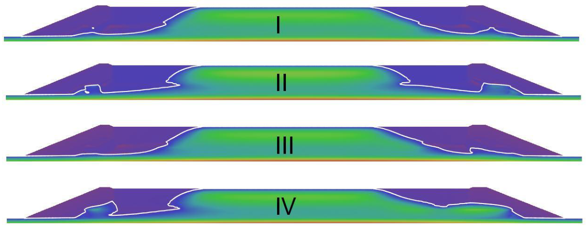
Setting II is imposed to simulate the effect of constructing the tailings beach with some mixture of total tailings and cyclone overflow, rather than total tailings alone, whereby the ratio of saturated horizontal hydraulic conductivity of cyclone underflow to adjacent tailings beach hydraulic conductivity is increased from 10 to 100 [15]. Setting III is imposed to simulate the reduction in void ratio of the 2011 downstream cycloned sand shell due to reactivated TSF construction [8]. The color coding in Figure 11 indicates different values of pressure head throughout the TSF, with the phreatic surface level in white corresponding to pressure head 0, violet/blue coloration of the downstream shells corresponding to saturation in the range of 0.2-0.4, and green coloration of the tailings slimes impoundment and tailings beaches corresponding to saturation 1 and approximately constant pressure head associated with a downward total hydraulic head gradient. Accordingly, the figure demonstrates how condition II influences phreatic surface level through the tailings beaches, and how conditions II and III together have a greater influence on dam crest phreatic surface level than conditions II or III alone. Given dam crest piezometer readings of approximately 900[m] for both the West or East Dam reported in 2024, and dam crest phreatic surface levels below 860[m] for simulations I, II, and III, these simulation results highlight the possibility that condition IV and/or perching/ponding of water near the dam crests is occurring [13].
Staged Construction Water Balance
Table 5 presents Case I annually averaged rates [day] of underdrain and foundation outflow, pond inflow, pond outflow, consolidation water inflow, and TSF total water content change including change in specific storage. The table demonstrates that for working underdrains, the West+East underdrain outflow is more than an order of magnitude greater than West+East foundation outflow bypassing the drains, and that the majority of seepage outflow is attributable to change in water storage of the dam shells and tailings beaches and consolidation water inflow rather than direct seepage from the tailings pond.
The 2D seepage analysis results, extruded to widths 250m and 750m, can be used to approximate lower and upper bounds on the 3D TSF design-intended underdrain and foundation flows. For 2025, the 2D staged construction seepage flows in Table 5 suggest lower and upper bounds on total underdrain and foundation flow are (657[day],1972[day])-West and (614[day],1842[day])-East, or (7.6[Ls],22.8[Ls])-West and (7.1[Ls],21.3[Ls])-East. More quantitatively, Figure 12 shows the end of 2025 3D phreatic surface through the TSF obtained by solving for the 3D RTF quasi-steady state in FEFLOW on a mesh with 46972 nodes and 230503 elements, for which total West and East foundation flows were computed to be 219.74[day] and 204.64[day]. Notably, these seepage flows are lower than the 2D RTF quasi-steady state seepage flows extrapolated to a dam width of 250[m], but greater than the 2D STF steady state seepage flows extrapolated to a dam width of 250[m], because the 3D RTF simulation was ran for more than 10 years to reach a true quasi-steady state condition. This quasi-steady state simulation result, as an approximation of a solution to the RTF equation for 3D staged construction seepage flow, highlights the possibility that 2019 reported total foundation flows of 60[L/s] and 130[L/s] for the West and East Dams are indicative of as-built TSF structural problems such as internal erosion [17]. 2D and 3D simulations performed with reduced underdrain hydraulic conductivity can further be used to analyze drain clogging problems that may be detected by piezometers in practice [16].
4. Discussion
While seepage analysis of TSFs often proceeds via solution of saturated flow equations, semi-analytic solution of Richards’ equation in 2D clarifies that differences can exist between RTF and STF solutions that may be relevant to slope stability factor of safety computations. In particular, 2D steady state solutions of the RTF and STF equations for seepage flow through an idealized tailings beach embankment have been verified against semi-analytic and analytic solutions, demonstrating differences between RTF and STF phreatic surface levels on the order of 10[m], and two orders of magnitude difference in transient decay time to steady state. Applied to analyze seepage through a TSF constructed by on-dam cycloning with long tailings beaches and a permeable foundation, FEFLOW 2D RTF simulation results demonstrate that phreatic surface, drain flows, and water balance can be computed with an accuracy useful for initial TSF dam design screening and highlighting possible as-built structural problems such as inadequate hydraulic segregation of tailings and internal erosion deserving of further attention by dam safety reviewers. While simulation results have been obtained for an idealized 2D TSF geometry with reference Van Genuchten parameters, it may be of value to perform a field study of tailings dam unsaturated flow parameters and obtain parallel results for more realistic 3D topography for more comprehensive design screening.
Funding
The author received no external funding for this research.
Statements and Declarations
The author declares they have no competing interests or funding.
Acknowledgments
Thanks to my family and DHI Group FEFLOW technical support.
References
- Blight, G.E.; Thomson, R.R.; Vorster, K. Profiles of hydraulic-fill tailings beaches, and seepage through hydraulically sorted tailings. J. S. Afr. Inst. Min. Metall. 1985, 85(5), 157–161. [Google Scholar]
- Brink, N.; Zurakowski, Z. Calibration of tailing consolidation parameters using field measurements. In Proceedings of the Tailings and Mine Waste 2020, Virtual Event, 2020; pp. 125–134. [Google Scholar]
- Caputo, J.J.; Stepanyants, Y.A. Front solutions of Richards' equation. Transp. Porous Media 2008, 74(1), 1–20. [Google Scholar]
- Celia, M.A.; Bouloutas, E.T.; Zarba, R.L. A general mass-conservative numerical solution for the unsaturated flow equation. Water Resour. Res. 1990, 26(7), 1483–1496. [Google Scholar] [CrossRef]
- Cherry, J.A.; Freeze, R.A. Groundwater; Prentice-Hall: Englewood Cliffs, NJ, 1979. [Google Scholar]
- Chetti, A.; Trouzine, H.; Korichi, K.; Hakmi, M.A. Investigation of numerical and analytical solutions of 1D steady and transient flow in unsaturated layered soils. Geol. Acta 2024, 22(8), 1–12. [Google Scholar] [CrossRef]
- Compère, F.; Kern, G.; Bellenfant, G. A 3D FEFLOW hydrogeological uranium underground mine model, France. In Proceedings of the FEFLOW User Conference, 2021. [Google Scholar]
- Das, B.M. Principles of Geotechnical Engineering; Cengage Learning: Stamford, CT, 2011. [Google Scholar]
- Farthing, M.W.; Ogden, F.L. Numerical solution of Richards' equation: A review of advances and challenges. Soil Sci. Soc. Am. J. 2017, 81(6), 1257–1269. [Google Scholar] [CrossRef]
- Fredlund, D.G.; Rahardjo, H.; Fredlund, M.D. Unsaturated Soil Mechanics in Engineering Practice; John Wiley & Sons: Hoboken, NJ, 2012. [Google Scholar]
- Gardner, W.R. Solutions of the flow equation for drying of soils and other porous media. Soil Sci. Soc. Am. J. 1959, 23(3), 183–187. [Google Scholar] [CrossRef]
- Harmony Gold Mining Company Limited: Harmony delivers phase 1 of Kareerand TSF extension on time and within budget. 2024. Available online: https://www.harmony.co.za/media/announcements/2024/ (accessed on 3 Mar 2026).
- Hudbay Minerals Inc.; Copper Mountain Mine (BC) Ltd. Copper Mountain Mine Tailings Management Facility 2024 Annual Facility Performance Report; Copper Mountain Mine, British Columbia, Canada, 2025. [Google Scholar]
- Huyakorn, P.S.; Pinder, G.F. Computational Methods in Subsurface Flow; Academic Press: New York, 1983. [Google Scholar]
- International Commission on Large Dams (ICOLD). Tailings Dam Design—Technology Update; Bulletin 121; ICOLD: Paris; 2019.
- Klohn, E.J. Seepage control for tailings dams. In Proceedings of the First International Conference on Mine Drainage; Miller Freeman Publications: San Francisco, 1979; pp. 671–725. [Google Scholar]
- Klohn Crippen Berger. Copper Mountain Mine (BC) Ltd.—Copper Mountain Mine Tailings Management Facility—2019 Integrated Life of Mine Plan Expansion Design; Technical Report prepared for Copper Mountain Mine (BC) Ltd., April 2020. [Google Scholar]
- Morgenstern, N.R.; Vick, S.G.; Viotti, C.B.; Watts, B.D. Report on the Immediate Causes of the Failure of the Fundão Dam; 2016. [Google Scholar] [CrossRef] [PubMed]
- Ormann, L.; Zardari, M.A.; Mattsson, H.; Bjelkevik, A.; Knutsson, S. Numerical analysis of strengthening by rockfill embankments on an upstream tailings dam. Can. Geotech. J. 2013, 50(4), 391–399. [Google Scholar] [CrossRef]
- Priscu, C. Behavior of Mine Tailings Dams under High Tailings Deposition Rates. Ph.D. Thesis, McGill University, Montréal, 1999. [Google Scholar]
- Tetra Tech Canada Inc. Copper Mountain Mine Tailings Management Facility 2021 Dam Safety Review; Report No. 704-ENG.VMIN03199-01; Tetra Tech Canada Inc.: Kelowna, BC, 2022. [Google Scholar]
- Tito, A.A. Numerical Evaluation of One-Dimensional Large-Strain Consolidation of Mine Tailings. Ph.D. Thesis, Colorado State University, Fort Collins, CO, 2015. [Google Scholar]
- Tracy, F.T. Clean two- and three-dimensional analytical solutions of Richards' equation for testing numerical solvers. Water Resour. Res. 2006, 42(8). [Google Scholar] [CrossRef]
- University of Pretoria; University of the Witwatersrand; Departments of Civil Engineering. Study into the Causes of the Jagersfontein Fine Tailings Storage Dam Failure on 11 September 2022; Report prepared for the Department of Water and Sanitation; 2024. [Google Scholar]
- Vereecken, H.; Kasteel, R.; Vanderborght, J.; Harter, T. Upscaling Hydraulic Properties and Soil Water Flow Processes in Heterogeneous Soils: A Review. Vadose Zone J. 2007, 6(1), 1–28. [Google Scholar] [CrossRef]
- Vick, S.G. Planning, Design, and Analysis of Tailings Dams; BiTech Publishers Ltd.: Vancouver, BC, 1990. [Google Scholar]
- Zhou, C.; Shen, Z.; Xu, L.; Sun, Y.; Zhang, W.; Zhang, H.; Peng, J. Global sensitivity analysis method for embankment dam slope stability considering seepage–stress coupling under changing reservoir water levels. Mathematics 2023, 11(13), 2836. [Google Scholar] [CrossRef]
Figure 1.
TSF (a) design layout, (b) 2D cross sectional geometry along the green longitudinal line, and (c) 3D geometry identifying where construction and foundation materials have been deposited within the sloping valley. Elevations of tailings impoundment surface 973[m], dam crest 983[m], and bottom of foundation 770[m] are indicated.
Figure 1.
TSF (a) design layout, (b) 2D cross sectional geometry along the green longitudinal line, and (c) 3D geometry identifying where construction and foundation materials have been deposited within the sloping valley. Elevations of tailings impoundment surface 973[m], dam crest 983[m], and bottom of foundation 770[m] are indicated.
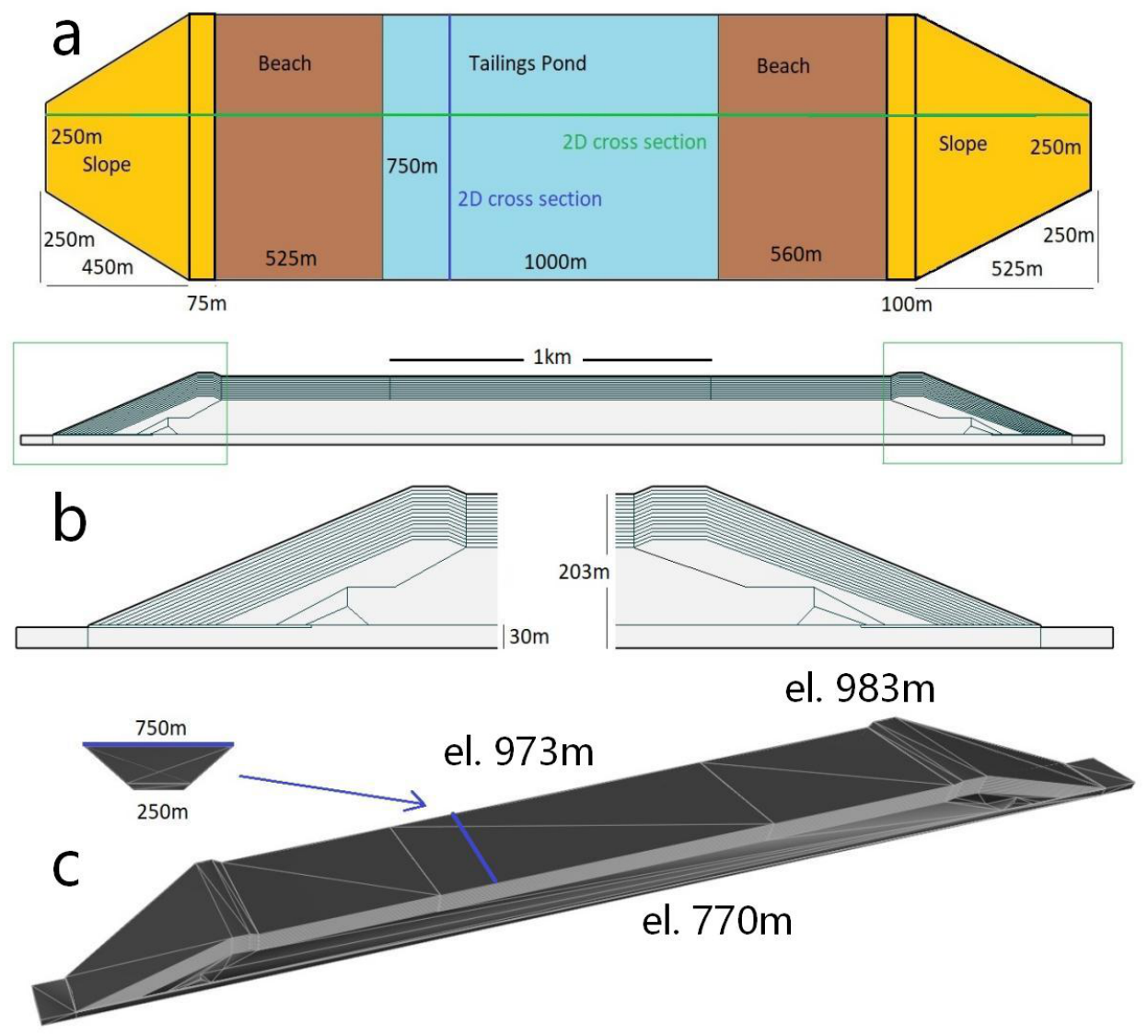
Figure 2.
Phreatic surface computation using Dupuit-Forchheimer approximation assuming saturated horizontal hydraulic conductivity and recharge rate of: (a)[m/s] and 0[m/year], (b)[m/s] and 2.5[m/year], (c)[m/s] and 0[m/year], and (d)[m/s] and 2.5[m/year].
Figure 2.
Phreatic surface computation using Dupuit-Forchheimer approximation assuming saturated horizontal hydraulic conductivity and recharge rate of: (a)[m/s] and 0[m/year], (b)[m/s] and 2.5[m/year], (c)[m/s] and 0[m/year], and (d)[m/s] and 2.5[m/year].
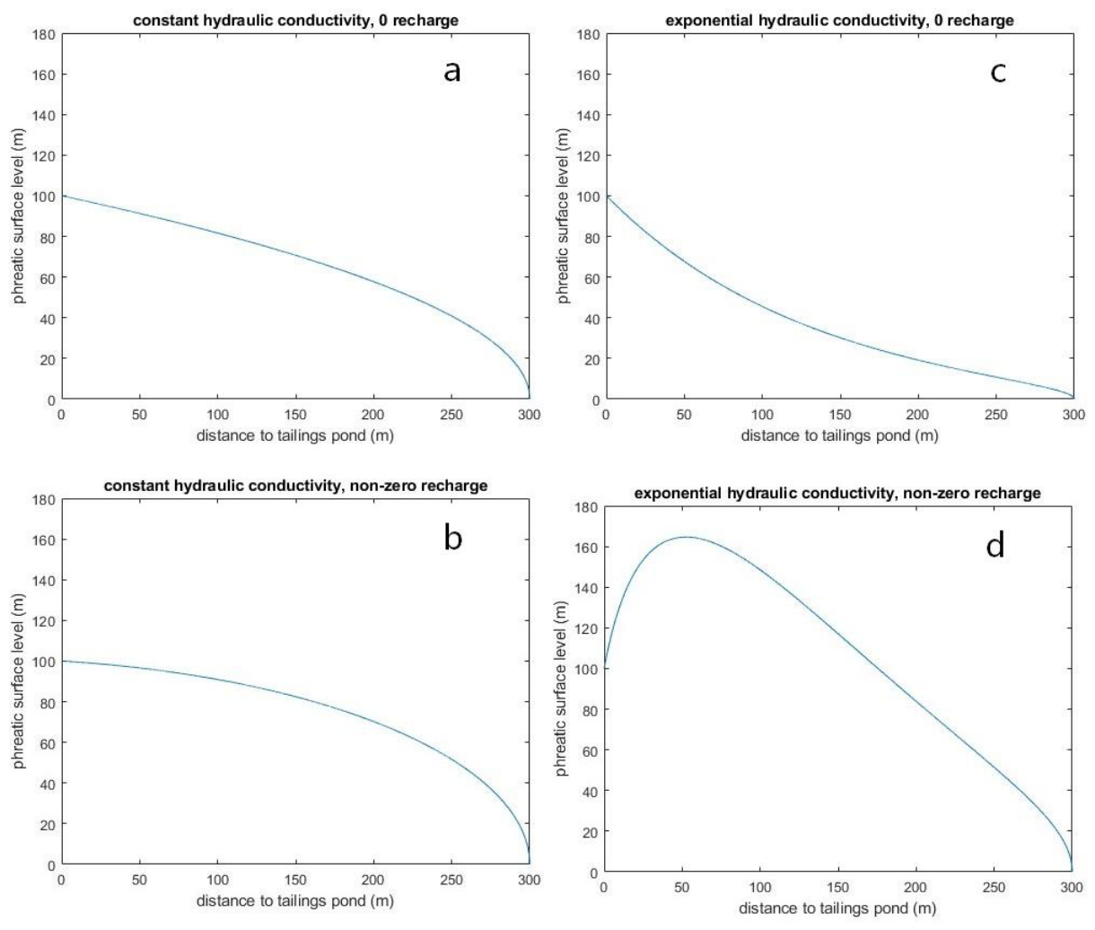
Figure 3.
Pressure head and water content profiles for 1D staged construction process with saturated vertical hydraulic conductivity [m/s].
Figure 3.
Pressure head and water content profiles for 1D staged construction process with saturated vertical hydraulic conductivity [m/s].
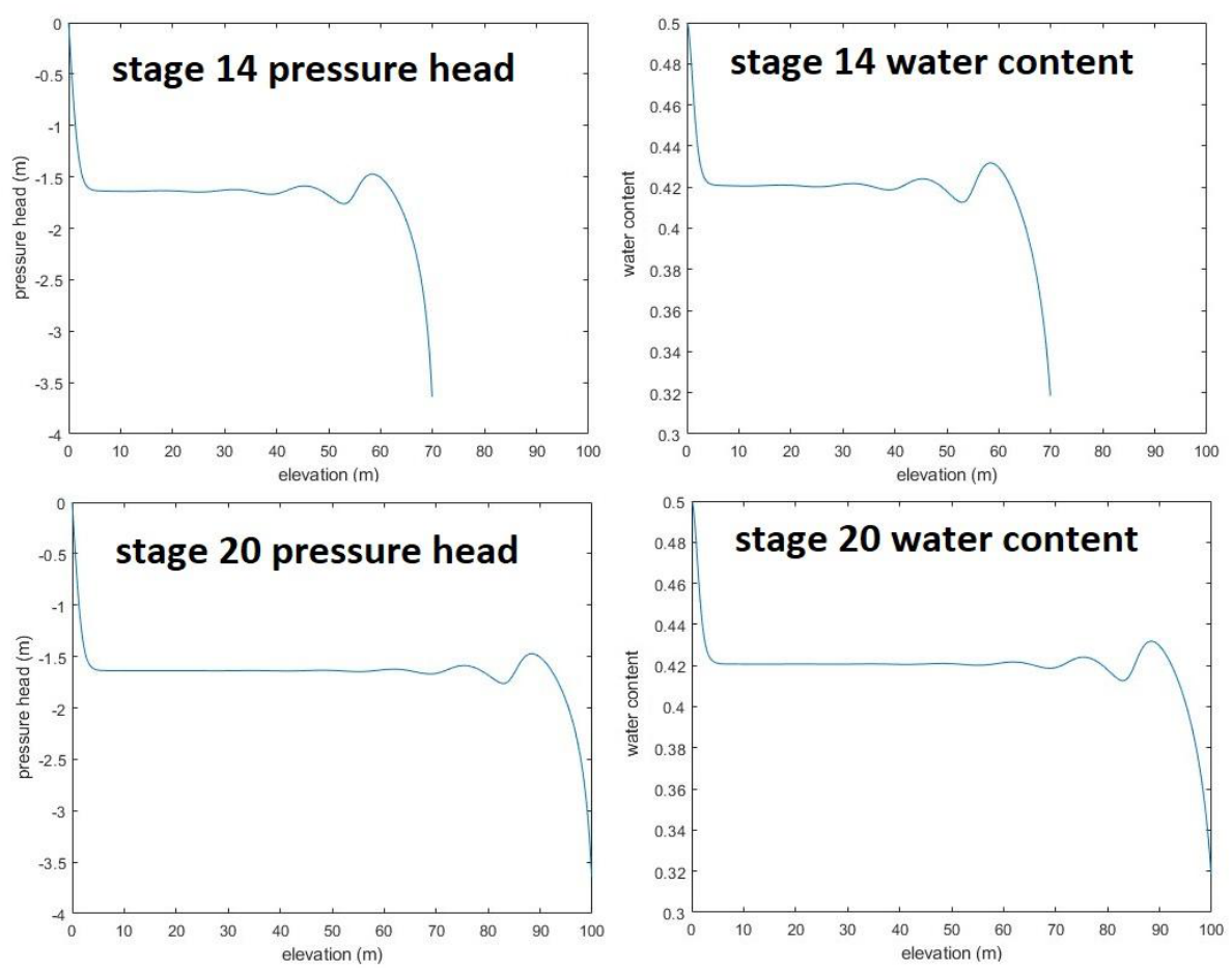
Figure 4.
(a) Water content and (b) annual average drain flow (stage 20) for 1D staged construction process plotted against saturated vertical hydraulic conductivity.
Figure 4.
(a) Water content and (b) annual average drain flow (stage 20) for 1D staged construction process plotted against saturated vertical hydraulic conductivity.
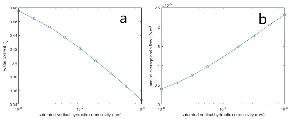
Figure 5.
Comparison of MATLAB finite difference and FEFLOW water content profiles through column of tailings beach material with [m/s] after stage 20. and correspond to water contents and for material porosity .
Figure 5.
Comparison of MATLAB finite difference and FEFLOW water content profiles through column of tailings beach material with [m/s] after stage 20. and correspond to water contents and for material porosity .
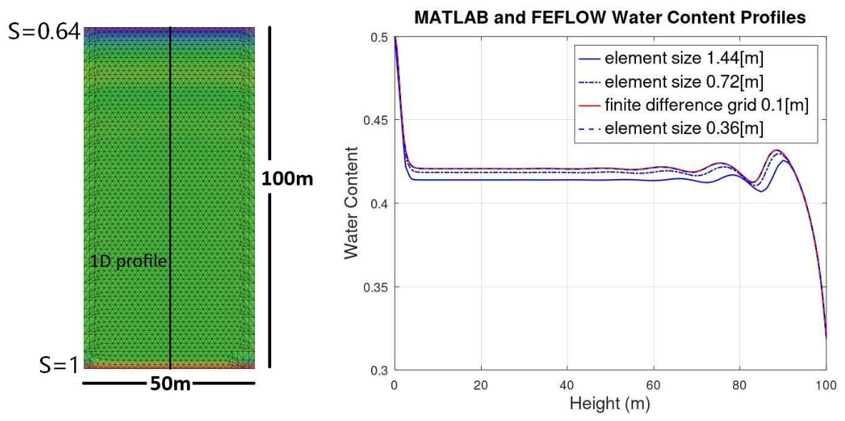
Figure 6.
Simulated (a) 1973-2025 tailings slimes impoundment total height and end of 2025 profiles of tailings slimes (b) saturated vertical hydraulic conductivity, (c) void ratio, and (d) excess pore pressure versus height.
Figure 6.
Simulated (a) 1973-2025 tailings slimes impoundment total height and end of 2025 profiles of tailings slimes (b) saturated vertical hydraulic conductivity, (c) void ratio, and (d) excess pore pressure versus height.
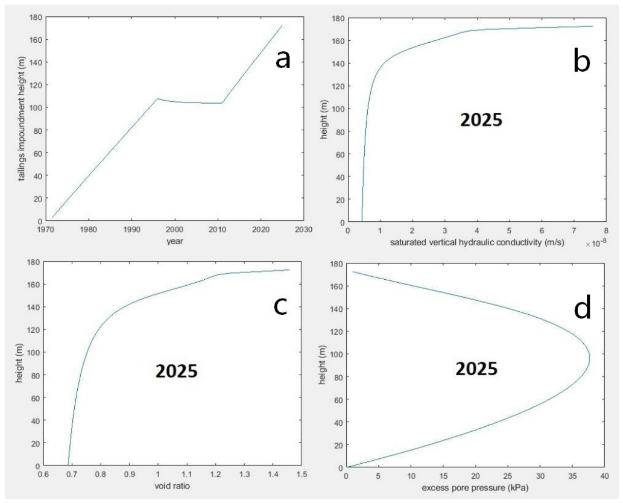
Figure 7.
Top: (a) RTF quasi-steady state and (b) STF steady state phreatic surfaces computed using FEFLOW. Bottom: (c) Plot of the perturbation quantifying where RTF and STF solution pressure heads differ for small .
Figure 7.
Top: (a) RTF quasi-steady state and (b) STF steady state phreatic surfaces computed using FEFLOW. Bottom: (c) Plot of the perturbation quantifying where RTF and STF solution pressure heads differ for small .
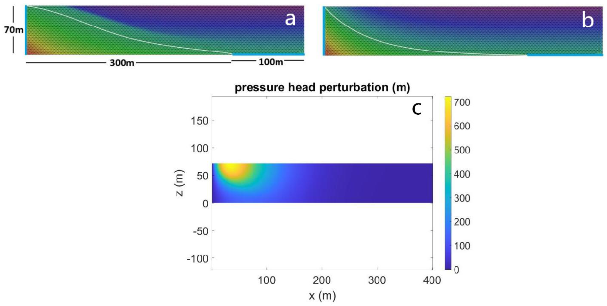
Figure 8.
(a) RTF transient solution water content and (b) STF transient solution average pressure head vs time plotted against exponential fit curves.
Figure 8.
(a) RTF transient solution water content and (b) STF transient solution average pressure head vs time plotted against exponential fit curves.
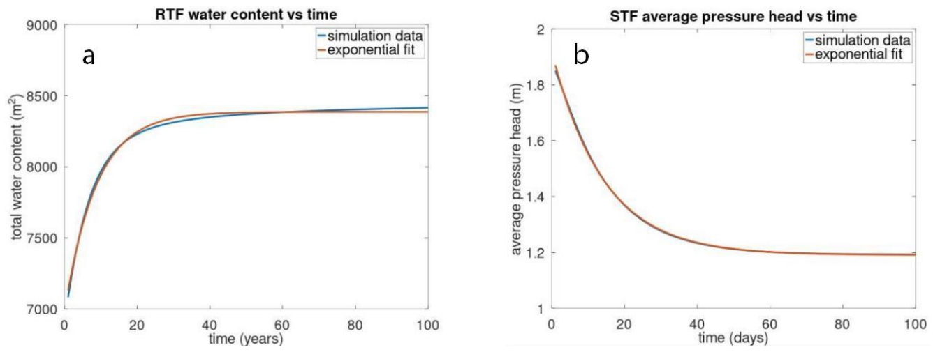
Figure 9.
Top: Staged construction RTF solution (a) phreatic surface and (b) saturation. Bottom: Final stage quasi-steady state RTF solution (a) phreatic surface and (b) saturation oscillations of the phreatic surface.
Figure 9.
Top: Staged construction RTF solution (a) phreatic surface and (b) saturation. Bottom: Final stage quasi-steady state RTF solution (a) phreatic surface and (b) saturation oscillations of the phreatic surface.

Figure 10.
End of 2025 TSF (a) quasi-steady state RTF and (b) steady state STF phreatic surfaces. .

Figure 12.
Influence of valley slopes on 3D phreatic surface through TSF and foundation flows approximated by solving the 3D RTF equation in FEFLOW for end of 2025 quasi-steady state flow.
Figure 12.
Influence of valley slopes on 3D phreatic surface through TSF and foundation flows approximated by solving the 3D RTF equation in FEFLOW for end of 2025 quasi-steady state flow.
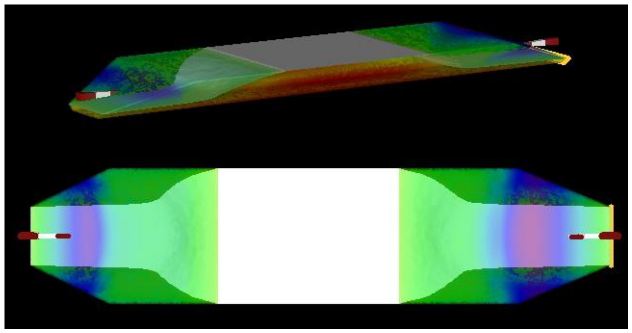

Table 1.
Typical saturated transient flow equation parameters for different tailings dam construction materials.
Table 1.
Typical saturated transient flow equation parameters for different tailings dam construction materials.
| Material | Conductivity [m/s] | Anisotropy / | Specific storage [1/m] |
|---|---|---|---|
| Uncompacted cycloned sand | 0.5 | ||
| Compacted cycloned sand | 0.5 | ||
| Starter dam (impervious) | 1 | ||
| Tailings beach | to | 0.2 | |
| Tailings slimes | to | 0.1 | |
| Foundation (sand/gravel/clay) | 0.01 | ||
| Underdrain (gravel) | 1 |
Table 2.
Typical Van Genuchten parameters for different tailings dam construction materials.
| Material | [1/m] | |||
|---|---|---|---|---|
| Uncompacted cycloned sand | 2 | 3 | 0.45 | 0.1 |
| Compacted cycloned sand | 2 | 3 | 0.4 | 0.1 |
| Starter dam (impervious) | 0.1 | 1.5 | 0.4 | 0.25 |
| Tailings beach | 0.5 | 2 | 0.45 | 0.15 |
| Tailings slimes | 0.1 | 1.5 | 0.4 to 0.6 | 0.25 |
| Foundation (sand/gravel/clay) | 2 | 2 | 0.35 | 0.1 |
| Underdrain (gravel) | 10 | 3 | 0.35 | 0.05 |
Table 3.
Mesh refinement effect on phreatic surface, drain flow, and water content. Mean and max absolute errors measured with respect to the element side length 0.36[m] RTF quasi-steady state solution.
Table 3.
Mesh refinement effect on phreatic surface, drain flow, and water content. Mean and max absolute errors measured with respect to the element side length 0.36[m] RTF quasi-steady state solution.
| Element Side Length [m] | Phreatic Surface Mean AE [m] | Drain Flow [] | Water Content Max AE |
|---|---|---|---|
| 1.44 | 0.52 | 0.329 | 0.21 |
| 0.72 | 0.14 | 0.332 | 0.03 |
| 0.36 | 0 | 0.334 | 0 |
Table 4.
Mesh refinement effect on TSF phreatic surface and total underdrain and foundation outflow. Mean absolute error measured with respect to the RTF quasi-steady state solution with 217044 elements.
Table 4.
Mesh refinement effect on TSF phreatic surface and total underdrain and foundation outflow. Mean absolute error measured with respect to the RTF quasi-steady state solution with 217044 elements.
| Number of Elements | Element Side Length [m] | Phreatic Surface Mean AE [m] | Total Outflow [] |
|---|---|---|---|
| 13647 | 5-30 | 4.4 | 2.85 |
| 54370 | 2.5-15 | 2.0 | 2.58 |
| 217044 | 1.25-7.5 | - | 2.42 |
Table 5.
TSF Water Balance Table. Quantities expressed in units [day].
| Stage | Underdrains | Foundation | Pond In | Pond Out | Consolidation | Total Water | Residual |
|---|---|---|---|---|---|---|---|
| 2012 | 2.25 | 0.29 | -0.90 | 0.00 | -0.28 | -1.20 | 0.16 |
| 2013 | 2.38 | 0.28 | -0.38 | 0.00 | -0.78 | -1.39 | 0.12 |
| 2014 | 2.55 | 0.27 | -0.19 | 0.00 | -0.93 | -1.62 | 0.09 |
| 2015 | 2.70 | 0.27 | -0.12 | 0.03 | -1.01 | -1.80 | 0.06 |
| 2016 | 2.87 | 0.27 | -0.12 | 0.06 | -1.06 | -1.98 | 0.04 |
| 2017 | 2.99 | 0.27 | -0.13 | 0.08 | -1.10 | -2.11 | 0.01 |
| 2018 | 3.26 | 0.30 | -0.13 | 0.10 | -1.13 | -2.41 | -0.02 |
| 2019 | 3.63 | 0.34 | -0.14 | 0.10 | -1.15 | -2.80 | -0.03 |
| 2020 | 3.94 | 0.36 | -0.15 | 0.10 | -1.18 | -3.12 | -0.03 |
| 2021 | 4.11 | 0.38 | -0.16 | 0.11 | -1.20 | -3.27 | -0.03 |
| 2022 | 4.26 | 0.38 | -0.16 | 0.10 | -1.21 | -3.41 | -0.03 |
| 2023 | 4.41 | 0.39 | -0.17 | 0.10 | -1.23 | -3.53 | -0.03 |
| 2024 | 4.54 | 0.40 | -0.18 | 0.10 | -1.25 | -3.64 | -0.04 |
| 2025 | 4.68 | 0.41 | -0.19 | 0.10 | -1.26 | -3.76 | -0.04 |
Disclaimer/Publisher’s Note: The statements, opinions and data contained in all publications are solely those of the individual author(s) and contributor(s) and not of MDPI and/or the editor(s). MDPI and/or the editor(s) disclaim responsibility for any injury to people or property resulting from any ideas, methods, instructions or products referred to in the content. |
© 2026 by the authors. Licensee MDPI, Basel, Switzerland. This article is an open access article distributed under the terms and conditions of the Creative Commons Attribution (CC BY) license (http://creativecommons.org/licenses/by/4.0/).
Copyright: This open access article is published under a Creative Commons CC BY 4.0 license, which permit the free download, distribution, and reuse, provided that the author and preprint are cited in any reuse.