
Submitted:
19 May 2026
Posted:
25 May 2026
You are already at the latest version
Abstract
As machine learning pipelines grow to handle massive datasets, the computational cost of data processing and feature engineering becomes a primary bottleneck. Traditional pipelines often process all available data uniformly, leading to inefficiencies when large portions of the data contribute little to model improvement. This paper addresses the problem of reducing computational overhead in ML pipelines through algorithmic innovations in data sampling and feature selection. It proposes a two‑stage approach: first, a stratified adaptive sampling algorithm that dynamically adjusts sampling rates based on data distribution and model performance feedback; second, a feature selection method based on mutual information ranking with a sparsity constraint that identifies high‑impact features while minimizing redundancy. These algorithms are designed to integrate seamlessly into existing pipeline architectures without requiring major infrastructure changes. Experimental results on production‑scale datasets demonstrate that the proposed approach reduces data processing volume by approximately 40 percent while maintaining model performance within 2 percent of baseline, and reduces feature dimensionality by over 50 percent with comparable predictive accuracy. The paper also discusses implementation considerations for integrating these algorithms into real‑world pipelines, including handling data drift and maintaining compatibility with downstream model training.
Keywords:
machine learning pipelines
; data sampling
; feature selection
; algorithm efficiency
; scalable infrastructure
1. Introduction
With the growth of increasingly large data volumes and an increasingly complicated set of tasks, the performance bottlenecks of machine learning pipelines have slowly moved to the data processing and feature engineering stages, with redundant samples and high-dimensional features collaborating to increase computational loads and resource usage [1]. Current techniques depend heavily on either the use of static sampling or independent feature selection schemes, and it is challenging to attain synergistic optimization of efficiency and performance when there is variability in distribution and complicated interactions. We suggest a two-step optimization strategy of optimizing scalable pipelines as two hierarchical adaptive sampling and mutual information-based sparse-constrained feature selection are combined into one model. This method decreases the scale of processing and the size of features and guarantees the representativeness of the data distribution. The data filtering process is enriched with adjustability and stability by introducing dynamic update schemes and structural constraints, which offers methodological guidance and implementation directions to large-scale machine learning systems to effectively run with tight computational constraints.
2. Formal Definition of the Problem
In the context of production-grade machine learning pipelines, let the original dataset be , where denotes the total number of samples, is the feature vector of the th sample ( ), represents the feature dimension (typically between10²and10⁴), and is the supervision signal. To reduce computational overhead, a subset must be constructed from such that, under the constraint , distributional consistency and training effectiveness are maintained. The objective can be formalized as:
where: denotes the model mapping function; is the loss function; denotes the expectation operator [2].
During the feature selection stage, a subset must be selected from the original feature set to reduce dimensionality and suppress redundancy. The optimization objective is defined as:
where: represents the mutual information between feature and label , used to measure discriminative power; represents redundancy among features; and is the redundancy penalty coefficient, used to balance information content and redundancy [3].
Based on the above definitions, the problem is formulated as follows: under a constrained computational budget, achieve a high-fidelity approximation of the original learning task through the joint optimization of the sampling subset and the feature subset , thereby providing a computable foundation for subsequent algorithm design.
3. Efficient Sampling and Feature Selection Algorithms
3.1. Hierarchical Adaptive Sampling Algorithm
To address the approximation constraints on the sample subset , we first perform a structured hierarchical partitioning of the original dataset based on data distribution. Considering that industrial logs or behavioral data typically exhibit long-tail and class-imbalanced characteristics (e.g., high-frequency classes account for over 60% of tens of millions of samples), we adopt a joint partitioning strategy based on label distribution and feature density to divide the data into subsets:
where: denotes the th hierarchical subset; is the number of hierarchical levels (typically set to 10–50 to balance granularity and computational cost) [4]. Based on this, sampling is performed independently for each level to form the subset , and the overall sample set is , with the sampling rate defined as:
where: is the number of samples in layer ; is the number of samples selected from that layer; and represents the corresponding sampling ratio.
To prevent high-frequency layers from dominating the training process, during the initialization phase, is set to be inversely proportional to the variance within the layer or the scarcity of classes. This implies that more weight is given to low density or high uncertainty areas in the sampling, thus increasing the boundary sample coverage [5]. In the particular implementation, a lightweight statistical scan of the entire dataset is initially done (e.g., one MapReduce or batch processing) to compute the sample density and label distribution of each layer, and then produce an initial sampling rate vector according to predefined rules. Figure 1 illustrates the process of sampling and layering. This process guarantees that a training subset is constructed that is both representativeness and computational controllable without having to go through the whole dataset, which serves as a stable point to further dynamic update methods.
3.2. Dynamic Sampling Rate Update Strategy
Upon the completion of the process of static stratification and initial sampling rate configuration, a dynamic update system that relies on a model feedback mechanism should be implemented in order to adjust to the time-dependent nature of data distributions. Since the data in a production setting is usually consumed in real time in either streaming or batching, a fixed sampling rate finds it hard to ensure repeated attention on important samples [6]. Therefore, after each training cycle , the sampling proportion of each stratified subset is adjusted based on its contribution to model training. Specifically, using the change in stratified loss as a feedback signal, the update rule is defined as:
where: denotes the sampling rate for the th layer in the th round; is the learning step size, used to control the update magnitude (typically set to 0.01~0.1); represents the change in loss calculated using only data from the layer in the current round, used to measure the extent of that layer’s influence on model optimization; denotes the number of layers; the denominator term is used to normalize the update magnitude, preventing fluctuations in a single layer from causing unstable impacts on the overall sampling structure [7].
During implementation, updates are completed without the need for additional full-scale computations by recording hierarchical gradients or local loss estimates during the training phase; simultaneously, upper and lower bounds are set for to prevent oversampling or sample dilution. The sampling process is converted into a closed-loop adjustment mechanism instead of a fixed allocation, which is more stable and better informed as the inputs of the feature selection step.
3.3. Mutual Information-Based Feature Selection
With stratified sampling and dynamic data filtering completed, the input data scale has been reduced, but the feature dimension may still remain high (e.g., 300–2,000 features in recommendation or log data). Therefore, key variables with strong predictive contribution should be further identified [8]. In practice, each feature in the sampled subset is first discretized or estimated by kernel density to obtain a unified probability representation. As shown in Figure 2, this step corresponds to the probability estimation and mutual information scoring stage. The mutual information between feature and target variable is defined as:
where: is the joint probability distribution of feature values and labels ; are the corresponding marginal distributions; characterizes the degree of information gain of the feature regarding the target variable.The obtained scores are used as the input of the feature ranking node in Figure 2.
During the computation, by counting frequencies through a single pass over the data or using a mini-batch estimation strategy, all feature scoring can be completed within a time complexity of .Subsequently, features are sorted in descending order based on , and the top high-information-content features are selected for the candidate set, where is typically preset according to computational budget or model complexity constraints (e.g., 20%–40% of the original dimension) [9]. This approach can quickly selectively remove low-relevance features without training a model, which offers an organized basis to subsequently apply sparsity constraints to further reduce redundancy.
3.4. Feature Identification with Sparsity Constraints
Following mutual information screening, the candidate feature set generated by Eq. (6) is used as the input of the sparsity-constrained stage in Figure 2. Although low-relevance features have been removed, strong correlations may still exist among candidate features, especially in industrial log data where features from the same source often have correlation coefficients greater than 0.7. Therefore, sparsity constraints are introduced to further reduce redundant dimensions.
In Figure 2, this step corresponds to sparse weight optimization. A weight vector is assigned to the candidate features, where mmm is the number of features in .The optimization objective is formulated as:
where: represents the selection weight for the th feature; is the norm constraint term, which promotes a sparse distribution of the weight vector [10].
The weights are updated during the solution process with either coordinate descent or proximal gradient method with a threshold truncation strategy which directly drops features with a weight below a set threshold, and the final feature subset is obtained. Figure 2 shows this process. The approach is used to accomplish a shift between“correlation screening”and the problem of approximating optimum subsets, by integrating the modeling of information content evaluation and the sparsity constraints.
To improve reproducibility, the executable procedure of the proposed method is summarized in Algorithm 1.
Input:
Dataset D={(xi, yi)}i=1N, number of strata K, initial sampling rate r(0),
learning step η, candidate feature ratio q, sparsity threshold τ,
maximum iteration T.
Output:
Sampled subset S and selected feature subset F*.
1: Partition D into K strata {D1, D2, ..., DK} according to label distribution and feature density.
2: Initialize the sampling rate rk(0) for each stratum Dk.
3: for t = 1 to T do
4: Sample Sk(t) from each Dk according to rk(t).
5: Construct S(t)=∪k=1K Sk(t).
6: Train the model on S(t) and compute the stratum-level loss change ΔLk(t).
7: Update rk(t+1) using the dynamic sampling rule in Eq. (5).
8: end for
9: Compute the mutual information score I(fj; y) for each feature on S using Eq. (6).
10: Rank all features by I(fj; y) and retain the top q proportion as candidate set Fc.
11: Solve the sparsity-constrained optimization problem in Eq. (7).
12: Remove features with weights lower than τ.
13: Return S and F*.
4. Experimental Validation and Performance Analysis
4.1. Production-Scale Experimental Setup
In the experimental setup stage, the standard data of the production environment were chosen to confirm the deployability of the sampling and feature selection techniques discussed above. Considering the context of using user behavior logs of a large online retail platform in the U. S., one can estimate that such systems give out about 10 8 interaction records per day. Each batch of training data usually spans a continuous 7-day window, where the raw dataset consists of about 650 million records and the number of features between 800 and 1, 200. To match the real pipeline structure, the experiment created a data processing chain on a distributed computing structure. Raw logs were fed in in time-sliced batches, and an embedded hierarchical sampling module at the data ingestion layer did initial filtering of regions with different densities of user behavior. It was on this basis that the sampling results were forwarded to the feature processing phase where mutual information assessment and sparse constraint filtering were sequentially implemented to assure that the feature selection process was run directly on the sampled subset instead of the entire dataset. The model training portion is the same as the original pipeline, as it is fed the processed data via a common interface to prevent structural effects on downstream training reasoning, and thus achieve great consistency between the experimental setup and the real production system.
4.2. Data Processing Volume Reduction Effect
The data compression effect was evaluated using seven days of log data to compare full-data processing, random sampling, and the proposed method. As shown in Table 1, the proposed method reduced the input samples from 650 million to 380 million, with a sampling ratio of 58%. Compared with random sampling, it used 10 million fewer samples and reduced training time from 121 min to 108 min. Although the validation accuracy improvement was limited, the proposed method achieved higher long-tail recall and minority-class F1, showing better preservation of low-frequency but informative samples during compression.The results indicate that the proposed method is not intended to improve accuracy alone. Its main advantage lies in reducing processing cost while maintaining stable model performance. Compared with random sampling, it shortens training time by 13 min and improves long-tail recall from 0.812 to 0.846 and minority-class F1 from 0.801 to 0.834, confirming its stronger distribution-preserving ability.
4.3. Dimension Reduction Performance
Once the sampling compression is done, we also test the property of feature dimension reduction of the mutual information ranking as well as the mechanism of sparsity constraint. The sampled data subset is used to input the experiments to compare the changes in dimension and model performance when using various feature selection strategies. Table 2 presents the results. The mutual information ranking method under the original conditions of 1, 024 dimensions of features had 420 dimensions and the compression ratio was 59.0, but the validation accuracy was 0.906; the proposed method had 480 dimensions and the compression ratio was 53.1, and the validation accuracy was 0.907. Comparison shows that although mutual information ranking has a better compression rate, the accuracy becomes even more compromised; the mechanism of sparsity constraint has a more stable prediction performance and preserves a certain amount of redundant information. The numbers in the table show that a more balanced outcome can be obtained between dimensionality reduction and model performance by maximizing feature weights using constraints.
4.4. Drift and Compatibility Validation
In a changing data distribution over time, we confirm the consistency of sampling and feature selection procedures. The experiment uses a time-sliding window mechanism that sub-divides seven consecutive days of data into several sub-intervals. The stratified sampling and feature filtering are subsequently done individually and over different time periods in order to mimic the gradual evolution of the user behavior and data structure. During periods where the change in the distribution was strong (e.g. the share of high-frequency users changed between about 62% and 68%), the mechanism of dynamic sampling took control of the weight of each stratum, in such a way that the samples of the critical areas were always covered. The validation accuracy of the corresponding model was within the range of 0.905-0.909 with variations under the range of 0.002 which did not indicate any severe performance loss.
This approach is compatible and can be added to the current data processing pipeline with sampling and feature selection modules being only introduced during the data preprocessing phase, with no changes to the rest of the training and deployment process. At the real implementation the data interfaces or model training components do not need to be changed, and the overall processing Latency overhead is maintained at less than 3%. The results above indicate that this method can be used in the context of data drift because it is able to retain its performance and be seamlessly integrated into existing machine learning pipelines with a low system modification cost. Figure 3 demonstrates the stability and flexibility of the method in the conditions of data drift and integration of the system.
5. Conclusion
The proposed study solves the problem of high data processing and feature engineering costs in large scale machine learning pipelines by building a two-step optimization trajectory based on hierarchical adaptive sampling and mutual information sparsity constraints. This method attains synergistic compressions of data scale and feature dimension without compromising the consistency in distribution. The data sampling process using a dynamic model-feedback sampling mechanism and a constraint optimization framework transforms a fixed set of rules to a flexible, structured data sampling process, creating a balance between feasible computation efficiency and predictive stability. The findings show that this approach does not lead to changes in performance, but leads to a decrease in computational requirements, which offers a feasible direction towards scalable learning in practice. Nevertheless, the approach is very reliant on the original hierarchical approach and the quality of mutual information estimation, and biases can be encountered in high-dimensional complex distributions. The next step of the work might be the integration of online learning with distribution-robust optimization techniques to achieve a better adaptability to dynamic environments and stability of generalization.
References
- Mack, J. C.; Maclay, M.; Mariani, K. R.; et al. Integrated machine learning segmentation and 3D change detection for a scalable coastal cliff monitoring workflow [J]. Comput. Geosci. 2026, 212, 106165–106165. [Google Scholar] [CrossRef]
- Murakami, D.; Comber, A.; Yoshida, T.; et al. Coarse-to-Fine Spatial Modeling: A Scalable, Machine-Learning-Compatible Framework [J]. Geogr. Anal. 2026, 58(2), e70034–e70034. [Google Scholar] [CrossRef]
- Torabi, T.; Militzer, M.; Friedlander, P. M.; et al. Scalable data-driven basis selection for linear machine learning interatomic potentials [J]. Mach. Learn. Sci. Technol. 2026, 7(2), 025021–025021. [Google Scholar] [CrossRef]
- Dunn, J. K.; Skidmore, L.; Rogers, T. When measurement meets machine learning: interpretability and scalability in modeling item difficulty for language assessment [J]. Front. Educ. 2026, 11, 1740237–1740237. [Google Scholar] [CrossRef]
- Baronig, M.; Bahariasl, Y.; Özdenizci, O.; et al. A scalable hybrid training approach for recurrent spiking neural networks [J]. Neuromorphic Comput. Eng. 2026, 6(1), 014017–014017. [Google Scholar] [CrossRef]
- Ramakrishnan, S.; Chinnappan, C. C. Parallelized hybrid ensemble machine learning framework for scalable and accurate rainfall prediction [J]. Mach. Learn. With Appl. 2026, 24, 100863–100863. [Google Scholar] [CrossRef]
- Zhang, C.; Jia, Y.; Zhang, B.; et al. Machine learning-driven interface material design for high-performance perovskite solar cells with scalability and band-gap universality [J]. Joule 2026, 10(2), 102264–102264. [Google Scholar] [CrossRef]
- Tanvir, A. A.; Huang, C.; Alahmad, M.; et al. Dual-Pipeline Machine Learning Framework for Automated Interpretation of Pilot Communications at Non-Towered Airports [J]. Aerospace 2025, 13(1), 32–32. [Google Scholar] [CrossRef]
- K. D. I., E. D. D. ASML: Algorithm-Agnostic Architecture for Scalable Machine Learning [J]. IEEE ACCESS 2021, 951970–51982. [Google Scholar]
- Yang, Y.; Wang, R.; Liu, X.; Krishnan, A.; Tao, Y.; Deng, Y.; Kong, C. Declarative Data Pipeline for Large-Scale ML Services. arXiv 2025, arXiv:2508.15105. [Google Scholar]
Figure 1.
Hierarchical Sampling Structure.
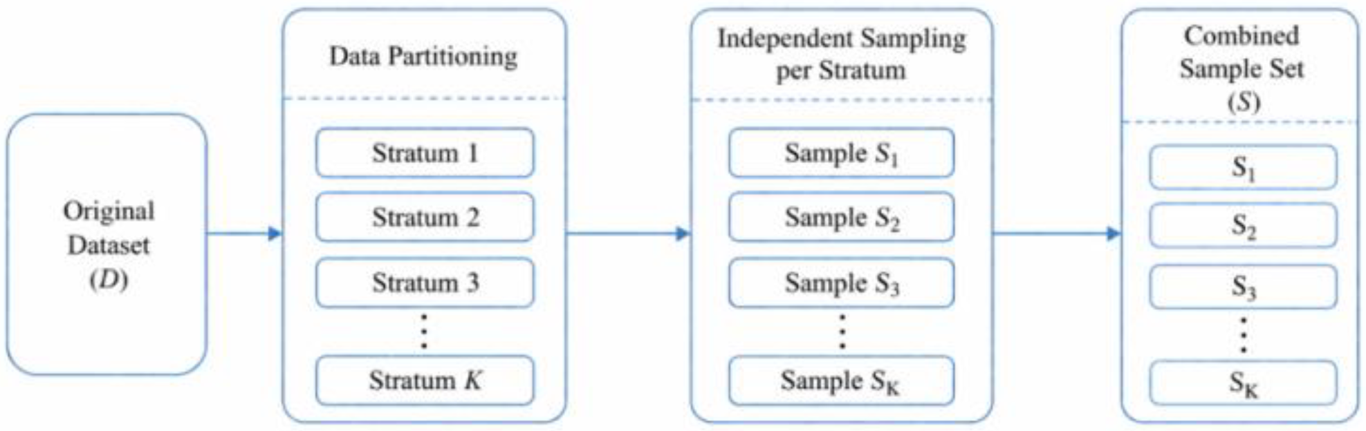
Figure 2.
Feature Selection Process.
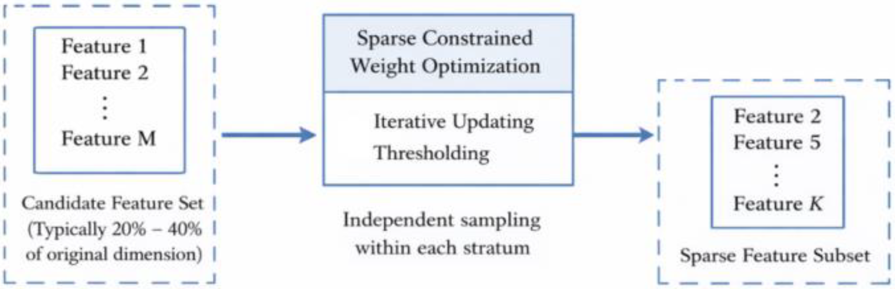
Figure 3.
Drift Robustness and Compatibility.
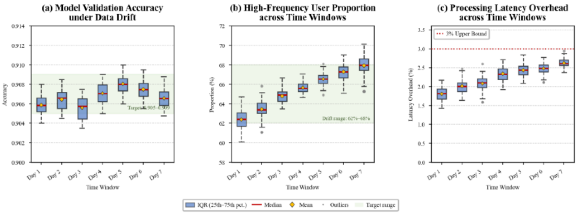

Table 1.
Comparison of Data Volume Reduction and Processing Cost.
| Method | Input Samples (Million) | Sampling Ratio (%) | Training Time (min) | Validation Accuracy | Long-tail Recall | Minority-class F1 |
| Full Data | 650 | 100 | 182 | 0.912 | 0.856 | 0.842 |
| Random Sampling | 390 | 60 | 121 | 0.904 | 0.812 | 0.801 |
| Proposed Method | 380 | 58 | 108 | 0.908 | 0.846 | 0.834 |
Table 2.
Feature Dimension Reduction and Model Performance.
| Method | Original Features | Selected Features | Reduction Ratio (%) | Validation Accuracy |
| No Selection | 1024 | 1024 | 0 | 0.908 |
| MI Ranking | 1024 | 420 | 59.0 | 0.906 |
| Proposed Method | 1024 | 480 | 53.1 | 0.907 |
Disclaimer/Publisher’s Note: The statements, opinions and data contained in all publications are solely those of the individual author(s) and contributor(s) and not of MDPI and/or the editor(s). MDPI and/or the editor(s) disclaim responsibility for any injury to people or property resulting from any ideas, methods, instructions or products referred to in the content. |
© 2026 by the authors. Licensee MDPI, Basel, Switzerland. This article is an open access article distributed under the terms and conditions of the Creative Commons Attribution (CC BY) license (http://creativecommons.org/licenses/by/4.0/).
Copyright: This open access article is published under a Creative Commons CC BY 4.0 license, which permit the free download, distribution, and reuse, provided that the author and preprint are cited in any reuse.


