Submitted:
21 May 2026
Posted:
22 May 2026
You are already at the latest version
Abstract
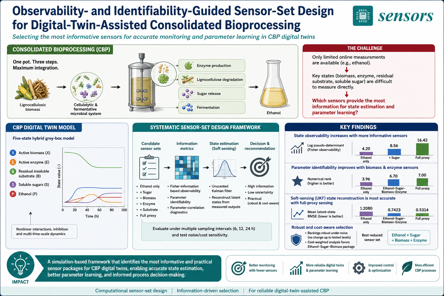
Consolidated bioprocessing (CBP) is difficult to monitor because enzyme production, lignocellulose degradation, sugar release, and fermentation occur simultaneously under sparse measurements, feedstock variability, and plant--model mismatch. This study proposes a computational sensor-set design framework for digital-twin-assisted CBP monitoring. A five-state virtual plant, consisting of active biomass, cellulolytic enzyme activity, remaining insoluble substrate, soluble sugars, and ethanol, was used to evaluate measurement packages ranging from ethanol-only sensing to full-proxy sensing. Candidate sensor sets were assessed using finite-difference output sensitivities, Fisher-information-based state observability and parameter identifiability analysis, parameter-correlation diagnostics, and unscented Kalman filter soft-sensing reconstruction. The results show that ethanol-only sensing is insufficient for state-aware CBP digital twins. At 6 h sampling, the state-observability log-pseudo determinant increased from 4.20 with ethanol-only sensing to 8.56 after adding soluble sugar, and to 16.42 with full-proxy sensing. Biomass and enzyme proxies contributed strongly to parameter learning, and the ethanol--sugar--biomass--enzyme package provided the best parameter identifiability across the sampling intervals. In the soft-sensing analysis, full-proxy sensing reduced the mean latent-state RMSE from 1.2080 to 0.5314 and gave the highest aggregate sensor value of 0.8144. The ethanol--sugar--biomass--enzyme package gave the best reduced sensor set, with a score of 0.7423 and lower measurement burden. Noise sensitivity analysis showed no ranking change under the tested noise levels, while cost-weight sensitivity analysis indicated ethanol--sugar--biomass as the preferred cost-sensitive package. The proposed framework provides a simulation-based method for prioritizing informative measurement packages before implementing CBP digital twins in laboratory and pilot-plant settings.
Keywords:
consolidated bioprocessing
; digital twin
; sensor-set design
; observability analysis
; parameter identifiability
; fisher information matrix
; soft sensing
; unscented Kalman filter
; hybrid grey-box model
; measurement uncertainty
1. Introduction
Consolidated bioprocessing (CBP) is a process-intensified route for producing ethanol and other biochemical products through the simultaneous biological integration of enzyme production, biomass deconstruction, and fermentation [1,2]. Its appeal lies in the potential to reduce dependence on externally supplied cellulases and to simplify the biomass-to-products chain compared with separated enzyme production, hydrolysis, and fermentation schemes. However, CBP remains technically challenging because its performance depends on host engineering, cellulosome biosynthesis, microbial consortia design, enzyme delivery, substrate accessibility, and feedstock deconstruction. Recent studies have therefore focused on CBP strains and genetic manipulation, synthetic cellulosomes and extracellular polymeric substances, microbial communities and co-cultures, enzyme delivery strategies, substrate accessibility, and process intensification [3,4,5,6,7]. From a monitoring perspective, CBP is not only a biochemical conversion process whose product yield should be maximized; it is also a nonlinear, partially observed dynamic system in which growth, enzyme synthesis, insoluble-substrate deconstruction, sugar release, sugar consumption, fermentation, and inhibition-related effects evolve on different time scales.
A central difficulty in developing digital-twin-assisted CBP is the limited availability of informative online measurements. Ethanol concentration is often one of the most accessible measurements, but it is a delayed product signal and cannot directly reveal whether poor batch performance originates from weak biomass growth, insufficient enzyme production, poor substrate accessibility, slow hydrolysis, sugar limitation, or product inhibition. In contrast, states that are more useful for process decision-making, such as living biomass concentration, active enzyme concentration, residual insoluble substrate, and soluble sugar concentration, are difficult to measure directly, continuously, or non-invasively. Similar measurement limitations have motivated the use of hybrid models, soft sensors, and online state-estimation methods in bioprocess monitoring and control [8,9,10,11]. Recent studies have also shown the value of soft-sensor recalibration, metabolic-heat-based soft sensing, spectroscopic monitoring, real-time biomass estimation, and Kalman-filter-based state–parameter estimation for improving the information content of bioprocess measurements [12,13,14,15,16,17,18]. In parallel, digital bioprocessing and digital chemical engineering studies emphasize accurate process measurements, model integration, predictive modelling, enabling digital technologies, and the progressive introduction of process analytical technology tools during process development [19,20,21,22,23,24,25]. For nonlinear systems, unscented Kalman filtering provides a convenient way to propagate uncertainty through nonlinear dynamics without local linearization [26,27]; therefore, the quality of soft sensing depends strongly on the informativeness of the available measurements.
The problem of choosing measurements for CBP cannot be reduced to the selection of a state-estimation algorithm. It is also necessary to determine whether the available measurements contain sufficient information for state reconstruction and parameter learning. State observability describes the extent to which hidden process states can be reconstructed from measured outputs, whereas parameter identifiability describes the extent to which model parameters can be estimated from available data. These concepts are especially important in partially observed biochemical systems, where unmeasured states and uncertain parameters can compensate for each other and produce similar measured trajectories [28,29]. Fisher-information and sensitivity-based metrics provide practical tools for quantifying measurement informativeness, observability, and identifiability. For CBP, this issue is particularly important because candidate measurements differ substantially in their measurement burden, cost, delay, and online implementation difficulty. For example, ethanol, soluble sugar, biomass proxies, enzyme-activity proxies, and residual-substrate proxies are not equally easy to obtain, and their value for digital-twin deployment should be evaluated before laboratory or pilot-scale implementation.
Although CBP has been widely studied from biological, biochemical, and process-intensification perspectives [3,6,7,30,31], systematic evaluation of measurement sets for CBP digital twins remains limited. Existing soft-sensing and bioprocess-control literature demonstrates that software sensors and nonlinear state-estimation methods can improve process monitoring [8,9,10,11]. More recent work has further highlighted the importance of soft-sensor generalizability, sensor recalibration, biomass monitoring, spectroscopic data streams, and joint state–parameter estimation for reliable model-assisted monitoring [12,13,14,16,17,18]. However, there is still no systematic comparison of CBP measurement packages with respect to state observability, parameter identifiability, soft-sensor reconstruction performance, measurement burden, and robustness to measurement uncertainty and alternative scoring priorities. In particular, it remains unclear whether ethanol-only sensing is sufficient for constructing a state-aware CBP digital twin, whether ethanol and sugar measurements provide an adequate minimal package, or whether additional biomass, enzyme, and substrate proxies are required.
To address this gap, this study proposes a computational framework for evaluating candidate CBP sensor sets according to state observability, parameter identifiability, soft-sensor reconstruction performance, measurement cost, and robustness to noise and scoring assumptions. A compact hybrid grey-box CBP model is used as a virtual plant for generating finite-difference output sensitivities, Fisher-information-based observability and identifiability scores, parameter-correlation diagnostics, and approximate uncertainty measures. The candidate sensor sets are then evaluated using a Monte Carlo unscented Kalman filter reconstruction test under model–plant mismatch and measurement noise. Finally, the sensitivity of the sensor-set ranking to measurement-noise scaling and alternative scoring weights is assessed.
The contribution of this paper is threefold. First, it provides a pre-experimental computational pipeline for ranking CBP measurement candidates before wet-lab or pilot-plant implementation. Second, it combines state observability and parameter identifiability analysis with soft-sensor performance rather than relying only on endpoint prediction or product monitoring. Third, it evaluates the robustness of the resulting sensor ranking with respect to measurement noise and alternative weighting of information, reconstruction, and cost criteria. The results are intended to support digital-twin readiness assessment and experimental planning for CBP, rather than to claim experimental validation of a specific organism or process.
2. Model, Sensor Sets, and Information-Based Analysis
2.1. Hybrid CBP Digital-Twin Model
A compact hybrid grey-box model was used as the computational digital-twin core for consolidated bioprocessing (CBP). The model was formulated to include the most significant dynamic couplings inherent to CBP, namely, growth of microorganism biomass, synthesis of cellulolytic enzymes, hydrolysis of insoluble substrate, accumulation and consumption of soluble sugars, and ethanol synthesis. Simplified mechanistic and hybrid models are common choices for bioprocess monitoring, state estimation, and control due to their interpretation potential and computationally-efficient structures [8,9,10]. In addition, modern bioprocess digital twins and hybrid models place particular emphasis on model compactness required for online state estimation and uncertainty analysis [11,19,20,32,33,34]. The state vector was defined as
where X is biomass activity, E is enzymatic activity, B is residual insoluble substrate, C is soluble sugars concentration, and P is ethanol concentration. The operating variables included temperature and pH:
The model described CBP as three continuously-varying regimes. The first one was the regime of growth and enzyme production; the second one was the regime of substrate hydrolysis; the third one was the regime of ethanol fermentation. This phase-based structure corresponds to the well-known view of CBP as a process consisting of four consecutive steps in which cellulase production, cellulose deconstruction, sugar release, and ethanol fermentation were performed in a coupled way in a single operation [30,31]. Contemporary works on CBP stress the role of this coupling in lignocellulosic conversion processes [5,6,7]. The phase weights were calculated using logistic functions:
where , h, and h. Normalization of the weight functions provided their summation to unity. It should be stressed that this formulation does not cover all the regulatory mechanisms within the process as it was intended for use as a controlled dynamic benchmark in which the latent states were characterized by different timescales and levels of measurement relevance for observability and identifiability assessment.
The equations describing the nominal behaviour of the system were written as
where was the biomass carrying capacity constant. All growth, enzyme, hydrolysis, and fermentation dynamics depended on temperature and pH activity profiles. Hydrolysis and fermentation rates were computed as follows:
where was a small constant ensuring division by a non-zero number. Hydrolysis rate increased with residual substrate amount and enzymatic activity but was also limited by the factor. Fermentation rate transformed soluble sugar into ethanol with a feedback-dependent effect on product-inhibition dynamics. Despite its simplicity, the model preserved the crux of the monitoring problem related to CBP: ethanol was a late product, and the reasons for poor batch performance could be traced in biomass, enzymes, substrate, and sugar states.
Seven log-multiplicative uncertainty factors were used to facilitate the parameter identifiability analysis:
They scaled growth rate, enzyme yield coefficient, hydrolysis capacity, ethanol yield, decay rate, inhibition rate, and feedstock accessibility, respectively. The logarithmic parameter transformation made sense due to multiplicative character of kinetic uncertainties and possible identifiability degeneracy under simultaneous effects of multiple biochemical mechanisms [28,29].
The assumed initial condition was
where and thus in the present study. The batch cycle duration was 96 h, while numerical integration was done by means of the fourth-order Runge–Kutta method with a 2-h internal time step. In order to conduct the observability and identifiability analysis, the open-loop control input was scheduled in such a way that all growth/enzyme synthesis, hydrolysis, and fermentation modes were activated:
This profile was not designed for optimal production of ethanol. The objective was to create a sufficiently representative trajectory to compare potential sensor suites. Excitation is vital in this respect as information-theoretic and sensitivity measures of identifiability are trajectory dependent [35,36]. In other words, the model can be considered an experimental template for sensor suite design but not as a fully developed organism-specific CBP model.
2.2. Candidate Sensor Sets and Measurement Assumptions
The sensor library included not only commonly made process measurements but also potential proxy measurements for latent CBP states. Five measurements were considered:
where P is ethanol, C is soluble sugar, X is a biomass proxy, E is an enzyme activity proxy, and B is a substrate proxy. Such an approach reflects the common monitoring problem in CBP where the product is straightforward to monitor while underlying biological and enzymatic states are sparse or difficult to monitor online. Soft sensing approaches and process analytical technologies have been proposed to overcome similar monitoring limitations in bioprocess development [8,9,10,11,19,24]. The nominal measurement standard deviations and relative costs are summarized in Table 1. Here, the cost represents a dimensionless estimate of the measurement burden related to sampling efforts, assay time latency, and online implementation difficulty rather than an exact cost amount.
Seven sensor sets were considered, from monitoring only product to monitoring all available states and proxies:
The ethanol-only set was taken as the baseline because it represents the most straightforward configuration. The ethanol-sugar set represented the most minimal biochemical measurements package. The other sets explored whether adding measurements of biological and hydrolysis proxies improved state observability and parameter identifiability. Such an approach helped to assess both the importance of monitoring product, biochemical intermediates, biological, and hydrolysis states. In addition, recent advances in soft sensing and state estimation in lignocellulosic and fermentation processes suggest such an approach is necessary, because hybrid sensors and state estimators rely heavily on which state variables are monitored [37,38,39].
Measurement sensitivities were computed with the sampling periods of 6, 12, and 24 h. They corresponded to increasingly sparse sampling scenarios in the lab and pilot plants. For a given sensor set and sampling period , the model outputs were obtained by concatenating the measurements made at each sample point into a single vector,
where denotes the selection of states corresponding to the sensors in the set . Each output component was weighted by the corresponding measurement standard deviation, thus more accurate measurement provided higher weights.
2.3. State Observability Analysis
State observability was determined by evaluating the sensitivity of the output vector to perturbations in the initial state. Given a sensor set , the finite-difference sensitivity w.r.t. to j-th initial state was estimated as
where is the j-th unit vector and is the state dependent perturbation,
When the perturbation was negative and caused violation of nonnegativity, the perturbation value was clipped and the actual perturbation distance was reported. Next, the matrix of weighted sensitivities was estimated as
where is the diagonal matrix of measurement standard deviations repeated over the whole time window.
Then, Fisher information was approximated by computing the matrix
This matrix cannot be considered the structural observability matrix in the pure differential geometric sense. Rather, it is a matrix of experimentally obtainable information about the initial states encoded in the measurements. This approach corresponds to Fisher information approximation, widely applied in analyzing observability of complex biological systems [29,35,36].
The following measures were taken from : numerical rank, log pseudo-determinant, minimal active eigenvalue, condition number, and correlation analysis. The log pseudo-determinant is calculated as
where are the eigenvalues of and is the numerical eigenvalue threshold. The minimal active eigenvalue, , denotes the direction with the weakest information content, while the condition number,
measures the level of anisotropy in the information content. The state covariance was estimated by means of a regularized pseudoinverse:
Using such criteria, sensor ensembles can be ranked not only based on their aggregate information quantity but also on whether some aspects of the system state remain ill-defined.
2.4. Parameter Identifiability Analysis
The problem of parameter identifiability was analyzed using an identical information-based approach, but with sensitivities computed with respect to logarithmically scaled model parameters instead of initial states. The parameter vector was
where all nominal values of the log-parameters were zero, corresponding to multiplicative scales of one. The finite difference derivative of the output vector with respect to the jth log-parameter was
The exponential mapping guarantees that variations are equivalent to relative changes in the kinetics and feedstock input terms. The weighted parameter sensitivity matrix and Fisher information matrix were
and
The same metrics for state observability were also computed for parameter identifiability. Approximate parameter uncertainty was derived from
with the standard error of the jth log-parameter estimated by
The associated approximate multiplicative 95% uncertainty factor was
Correlations between parameters were defined by
Large off-diagonal correlation factors denote parameter pairs that are problematic to estimate due to their non-separability using the proposed measurements. In this context, the issue of non-identifiability is relevant for partially observed bio-processes, for which alternative kinetic models could result in nearly identical observed ethanol or sugar time courses. In cases where the data obtained is scarce, noisy, or lacks diversity [28,29], identifiability analysis plays the role of a computational filter that aids in choosing the packages of CBP measurements that have potential for useful parameter inference.
3. Soft-Sensor Evaluation, Sensor Ranking, and Robustness Assessment
3.1. Soft-Sensor Reconstruction Test
After the observability and identifiability analyses, each candidate sensor set was evaluated for nonlinear soft-sensing reconstruction under modelling errors, initial-state uncertainty, and measurement noise. An unscented Kalman filter (UKF) was used because it can propagate mean and covariance information through nonlinear and phase-dependent dynamics without local linearization, which is important when some process states are only partially measured. Recent bioprocess monitoring studies emphasize that soft sensors, hybrid models, and model-based state-estimation methods are essential for digital bioprocessing because key physiological states are often unavailable from direct online measurements [11,37,38,39,40]. Related work on sensor-assisted bioprocess monitoring has also demonstrated the value of metabolic-heat-based soft sensing, spectroscopic monitoring, biomass estimation, soft-sensor recalibration, and joint state–parameter estimation for improving process-state reconstruction [12,13,14,15,16,17,18].
For the five-state CBP model, the UKF estimates and covariance matrices at time are denoted by and , respectively. The sigma points are generated as follows,
with and
The UKF parameters are , , and . Every sigma point was propagated over one plant step using the fourth order Runge–Kutta integration scheme used previously in the plant,
where represents the CBP model integrated over the time-step. The predicted mean and covariance for the next step would be
and
where Q is the process noise covariance matrix and and are the conventional UKF mean and covariance weights respectively.
At the sampling instants, the measurement function used at each iteration considered states corresponding to sensor set :
where is the diagonal covariance matrix associated with the measurement noise. The predicted measurement sigma points and mean were given by
and
The innovation covariance matrix and state–measurement cross-covariance matrix were calculated via
Kalman gain and measurement update step were done as follows:
The use of the pseudoinverse matrix helped ensure numerical stability.
The estimation accuracy was checked via Monte Carlo simulation experiment. For each sensor set configuration, simulation experiments were run. For each simulation run, multiplicative mismatch was assumed for growth, enzyme yield, hydrolysis capacity, ethanol yield, decay, inhibition, and feedstock accessibility parameters. The UKF used the nominal model and thus could not know about any perturbation specific to the actual plant. Similarly, initial-state uncertainty was induced through deviations in the estimator’s initial state relative to the true initial state of the plant. Such a design captures the real-world scenario where the mathematical structure of the model is known, while the plant parameters and its initial state remain uncertain.
In each experiment, the reconstruction error of state j was defined as
where r indicates the index of the experiment, and represents the total number of time instances within the simulation. Latent-state RMSE was computed across the non-product states as
However, ethanol was not considered in calculating the average above since it is always measured using any combination of sensors and hence poses no challenge regarding reconstructing a hidden state. Some other statistics calculated include the absolute estimation error at the end of the time horizon,
mean absolute error, and the trace of the covariance matrix at the final step,
Comparison between each non-baseline set of sensors and ethanol-only monitoring was made via the replicate-specific latent-state RMSE values. The difference in comparison to the baseline was calculated by
where a positive value of denotes smaller reconstruction error compared to the baseline. Because the signed-rank test is a nonparametric test that does not assume normality of RMSE differences, it was employed as an additional analysis [41]. The test was not used to rank the sensors, as its purpose was only to serve as an additional analysis to the information-based/reconstruction-based sensor value assessment.
3.2. Scoring Sensor Values and Rankings
The last step in assigning sensor rankings considered four factors in concert: state observability, parameter identifiability, UKF reconstruction accuracy, and cost. Since each quantity has units and spans a different range, normalization was applied to transform their ranges to lie in the unit interval . For a metric for which higher values are desirable, the normalized score is defined as follows:
Whereas a score for a metric with low preference was calculated as:
In case the range was zero, the normalized scores of all sensor sets were set to 0.5. This method, commonly known as min–max normalization, is an efficient way to rank different sensors according to multi-factor criteria by putting information value and measurement cost on the same scale. The idea behind composite scoring is extensively utilized when designing experiments in which informativeness, uncertainty reduction, robustness, and engineering constraints play equally important roles [11,24,35,36].
To rank a sensor set with regard to observability, the amount of information provided by the measurements and the quality of information in the worst resolved state directions were considered:
Similarly, parameter identifiability was ranked using a linear combination:
Here, the pseudo-determinant factor incentivizes total information volume, while the minimum-eigenvalue factor penalizes configurations that do not provide adequate information for at least one state or parameter. This helps to avoid a situation where a sensor set can receive a very high information score based purely on its performance in a few selected directions.
The UKF reconstruction score was derived from the Monte Carlo average latent-state RMSE:
with being the mean latent-state RMSE across Monte Carlo runs. Finally, the measurement burden score was
with being the cost index of sensor set .
The overall score was given by
In this expression, the identifiability factor received a marginally larger weight than the observability factor, since the envisioned applications of the framework include both state reconstruction and digital twin learning with parameter refinement. The cost term was included to prevent a bias toward the most measurement-intensive solution.
A second measure of value per unit cost was calculated:
This score was not used as a criterion for ranking. It was used to analyze the trade-offs between information gain and measurement burden. The best-scoring full sensor suite can be characterized as the one with the highest total score, while the best-scoring subset could be defined as a high-score configuration that avoids the full measurement burden associated with measuring five states.
3.3. Noise and Cost-Weight Sensitivity Analyses
A robustness analysis was done to assess whether the sensor set hierarchy strongly depends on either the measurement quality assumption or on the choice of score weights. Robustness analysis is important since the quality of measurements, cost per assay, as well as the relative significance of observability, identifiability, and reconstruction performance can vary greatly among laboratories and development stages.
For this purpose, a measurement noise sensitivity analysis was done using three uniform noise multipliers :
In this experiment, all nominal values of the sensor standard deviations are scaled as follows:
Finally, weighted sensitivity matrix and the corresponding metrics of information gain were recalculated. Since Fisher information gain explicitly depends on noise scaling, this experiment tests whether the order of the sets remains the same.
The second step was a reevaluation of the aggregate score using alternative weighting schemes. For each weighting scheme, let
In this notation, the total score was calculated as follows:
A few alternative weight vectors were considered:
These cases correspond to various criteria: balanced performance, observation-oriented design, identification-oriented design, reconstruction-oriented design, cost-sensitive preference, and cost-averse preference.
The robustness evaluation under noise and weight variation was conducted as a computational benchmarking test for the proposed ranking criterion. A CBP sensor suite that maintains high ranking for all noise levels and weight schemes is more likely to be a preferred choice for pre-experimental CBP digital twin design. On the other hand, a preferred CBP sensor suite at one specific weight scheme should be considered objective-specific, not necessarily optimal.
The workflow for pre-ranking CBP sensors prior to individual modeling and analysis is presented in Figure 1.
3.4. Computational Reproducibility
All simulations, state-estimation routines, sensitivity analyses, statistical comparisons, tables, and figures were implemented in Python 3.13.5 using a fixed random seed of 42. The final production run for this paper was executed from the Visual Studio Code integrated terminal and used NumPy 2.3.5, pandas 2.2.3, Matplotlib 3.10.8, SciPy 1.17.0, OpenPyXL 3.1.5, and PyTorch 2.10.0. The hybrid CBP virtual plant was simulated using a fixed-step fourth-order Runge–Kutta scheme. The same numerical integration approach was used consistently for trajectory simulation, finite-difference sensitivity analysis, and UKF prediction. The production run used Monte Carlo replicates for each candidate sensor set.
4. Results and Discussion
4.1. Nominal CBP Trajectory Under the Excitation Schedule
As expected, the nominal CBP trajectory under the excitation temperature-pH profile yielded phase-dependent responses (Figure 2). Biomass and enzymes increased in the early phase, hydrolysis caused soluble sugar accumulation in the intermediate phase, and ethanol production dominated in the later phases. Consistent with the view of CBP as a coupling of several processes, namely growth, enzymatic activity, deconstruction, sugar release, and product generation, occurring within different time scales [6,7,30,31], the delayed appearance of ethanol shows that its concentration is insufficient to characterize previous steps involved in bioconversion.
4.2. State-Observability Enhancement with Increasingly Informative Sensors
With an increasing number of sensors, state observability information was enhanced (Figure 3). Monitors consisting of ethanol provided relatively little information content in all sampling periods. Adding soluble sugar to the ethanol monitor was shown to significantly increase observability with log pseudo-determinant rising from 4.20 to 8.56 with 6 h sampling period. Further addition of biomass and enzyme monitors further enhanced state observability to a level of 16.42, 15.06, and 13.81 at 6, 12, and 24 h, respectively, whereas adding insoluble substrate proxy resulted in the least observable states due to its relatively low contribution to CBP process dynamics.
In summary, the proposed method is able to help select more effective monitoring sensors that go beyond traditional product-only measurement for CBP digital twin. This result is consistent with findings in other areas of bioprocess monitoring, where it is challenging to infer hidden physiological states based only on end-point data, whereas monitoring intermediates and using proxies can greatly improve soft-sensor performance [8,9,10,11]. The combination of ethanol, sugar, biomass, and enzyme was found to be sufficient for achieving almost optimal state observability without using the less useful residual substrate proxy.
4.3. Parameter-Identifiability Improvement with Biomass and Enzyme Sensors
Unlike state observability, the pattern of information gain regarding parameter identifiability showed a preference for the ethanol-sugar-biomass-enzyme monitor set (Figure 4) rather than the full proxy monitoring. Specifically, the log pseudo-determinants with ethanol-sugar-biomass-enzyme monitors were 10.83, 9.06, and 6.70 at 6, 12, and 24 h sampling periods, respectively, compared to those for full proxy monitoring being 8.69, 6.63, and 3.96, and the numerical identifiability rank also showed variation in relation to sensor type and sampling interval (Figure 5).
While observability and identifiability information may share many similarities, the difference is significant. An effective sensor configuration for improving state reconstruction does not imply that the same configuration is optimal for improving parameter identification because identifiability depends on how distinct responses the system is able to generate from parameter variations. For instance, in the current case where biomass and enzyme concentrations were considered as additional measurements, such information could complement each other in separating kinetic models of growth, enzyme yield, and hydrolysis processes from the model of ethanol inhibition, yield, and feedstock degradation.
The inclusion of biomass and enzymes surrogates lowered the uncertainty of parameters related to growth, enzyme yield, and hydrolysis processes (Figure 6). However, highly correlated parameters were still observed within selected pairs (Figure 7), namely, growth and decay, ethanol yield and inhibition, as well as hydrolysis ability and feedstock accessibility. In summary, even though enhanced proxy observation increases parameter reliability, not all non-uniqueness issues could be avoided since some biological processes still have equivalent responses in terms of output trajectory. Therefore, Fisher information and parameter correlation diagnostics serve as valuable tools prior to sensor placement in experiments [28,35,36].
4.4. Impact of the Sensor Set on the UKF Reconstruction Quality
It was demonstrated that more informative sensor sets resulted in better estimation of the latent state vector in the case of model–process mismatch. The weakest reconstruction performance was observed for ethanol-only monitoring and manifested itself as the highest RMSE of the latent state equal to 1.2080. By introducing a soluble sugar sensor, the RMSE dropped to 1.0434, which did not yet allow to fully reconstruct the values of the hidden biomass, enzyme, and residual substrate. The improvement in state-wise performance corresponded to their observation. Namely, the addition of a biomass proxy decreased the RMSE of the biomass estimation from 0.94 to 0.11, the addition of an enzyme proxy lowered the RMSE of the enzyme from 0.42 to 0.07, while the inclusion of the substrate proxy led to a decrease in RMSE from 3.15 to 1.24. Such tendencies are consistent with the observability analysis results and are corroborated by the previous studies of bioprocess soft sensing, which proved that the estimator’s quality critically depends on the availability of information about the direction of latent variables changes [8,9,10,11]. Statistical distributions of RMSE obtained via Monte Carlo simulation and mean errors for each state are depicted in Figure 8 and Table 2, respectively.
Paired Wilcoxon tests were conducted to compare each setup against ethanol-only monitoring on the assumption that RMSE differences are not normally distributed [41]. The largest reduction was achieved by full proxy monitoring, where the mean latent-state RMSE was lowered from 1.2080 to 0.5314 (). In addition, the setups involving ethanol, sugar, and either substrate and/or biomass and enzyme also showed significant improvements with and , respectively (Table 3).
4.5. Recommended Sensor-Set Ranking and Measurement-Burden Trade-Off
With respect to the aggregate sensor-value score, full proxy monitoring gave the highest overall score, followed by ethanol-sugar-biomass-enzyme and ethanol-sugar-biomass monitoring packages (Table 4). On the other hand, ethanol-only monitoring proved the least efficient, indicating the inadequacy of pure product-only sensing when state-reconstruction and parameter learning have to be taken into account. This result further reinforces the digital bioprocessing paradigm, according to which the integration of process analytical measurements, estimation techniques, and uncertainty-aware decision support precedes the deployment of closed-loop digital twins [11,19,20,24].
This ordering reveals the tradeoff between the two criteria. Total proxy monitoring produced the highest overall score yet also entailed the highest cost index. The ethanol-sugar-biomass-enzyme combination kept most of that advantage yet did so at a significantly lower cost, making it the top choice in reduced monitoring. The ethanol-sugar-biomass combination yielded the best relative compromise among the important multi-sensor options by achieving the highest value per cost ratio.
4.6. Robustness to Measurement Noise and Scoring Weights
Noise sensitivity analysis revealed the stability of the ranking when a uniform change is made on measurement noise assumption. Full proxy monitoring kept its lead in both low-noise, nominal-noise, and high-noise scenarios (Figure 9; Table 5). The Spearman rank correlation compared to the nominal ranking is 1.0 in all cases, without any shift in ranks. While the top score decreases slightly from 0.8235 at low noise to 0.8052 at high noise, there was no change in the order of sensors. Robustness to sensor quality, assay uncertainty, and data availability is vital for digital bioprocesses [11,19,24].
The analysis on weight sensitivity showed that only the change in the optimization objective caused a change in the preference of sensor set (Figure 10; Table 6). Under all formulations, except when parameter identifiability was the highest priority, full proxy monitoring emerged as the most attractive sensor set. When parameter identifiability took the lead, the second-best combination emerged as the most favorable one. In a strongly cost-averse formulation, full proxy monitoring became less preferred than the next-best sensor sets. These findings help to distinguish three practical objectives: maximizing available information, maximizing learning potential, and minimizing sensor burden [19,20,25].
4.7. Implications for Practical CBP Digital-Twin Development
These results support a hierarchical approach to measurement selection for CBP digital-twin development. Ethanol-only monitoring is the least informative configuration because ethanol is a delayed product signal and cannot indicate whether limited batch performance originates from biomass limitation, enzyme insufficiency, substrate scarcity, slow hydrolysis, sugar accumulation, or product inhibition. This is consistent with bioprocess soft-sensing studies showing that delayed quality indicators and hidden physiological states can limit real-time monitoring and control [8,9,10,11,42].
Adding soluble sugar provides a useful low-cost improvement because sugar links substrate hydrolysis to ethanol formation. However, the ethanol–sugar package should be regarded as a minimal measurement configuration rather than a complete digital-twin sensor package, since it does not directly capture biomass growth, enzyme activity, or residual substrate availability. This interpretation is consistent with process analytical technology and digital-bioprocessing approaches, where intermediate measurements are informative but often need to be combined with soft sensors, model-based estimation, and digital-twin architectures [11,19,22,24,43,44].
The most informative reduced measurement package is the ethanol–sugar–biomass–enzyme set. Biomass provides information about the biological state of the process, whereas enzyme activity provides information about hydrolytic capability. Their combined inclusion improves both state observability and parameter identifiability without requiring the full measurement burden associated with all proxies. Full-proxy monitoring is preferred when the highest information content is required, while the ethanol–sugar–biomass–enzyme set is more appropriate for parameter learning and model-refinement studies. Under strong cost constraints, the ethanol–sugar–biomass package provides a practical compromise. This staged interpretation agrees with recent sensor-centered bioprocess monitoring studies, which emphasize that physical measurements combined with software-sensor or model-based layers can improve process understanding and support more informative decision-making [42,44].
In practice, low-cost screening experiments could begin with ethanol–sugar–biomass measurements, while model-refinement experiments should include enzyme activity to improve the identifiability of growth- and hydrolysis-related parameters. High-quality benchmark experiments should use full-proxy monitoring when the measurement burden is acceptable. This staged development route is consistent with digital-bioprocessing and digital chemical engineering roadmaps, in which digital twins evolve through improved modelling, state estimation, process analytics, enabling digital technologies, and control-oriented decision support [19,20,21,23,24,25,43,44].
The proposed ranking should therefore be interpreted as a pre-experimental design result based on computational analysis. Different model structures, excitation schedules, sensor costs, and scoring priorities may alter the exact ranking. Nevertheless, the robustness analysis indicates that the main hierarchy is stable under uniform noise scaling and changes in a physically meaningful way when the scoring objective is shifted.
4.8. Limitations
Several limitations apply to the current work. First, the computational virtual plant was used to generate the observations and perform the analysis, without experimental data. The findings therefore provide guidance for sensor-set design and digital-twin readiness evaluation, but they do not represent experimental validation. Real CBP systems may involve organism-specific regulation, feedstock variability, mass-transfer limitations, inhibitor formation, contamination, evaporation, measurement delay, and assay-specific bias. Future work should verify the proposed hierarchy using synchronized measurements of ethanol, dissolved sugars, biomass proxies, enzyme activity, and remaining solids.
Second, the five-state hybrid system is a concise representation of lignocellulosic CBP. It captures the information flows required to analyze observability and identifiability, but it does not resolve all biochemical details. Extended models could explicitly include cellulose, hemicellulose, glucose, xylose, cellobiose, enzyme classes, inhibition mechanisms, and organism-specific metabolic states. Such refinements could change the relative importance of the candidate sensors and may introduce additional identifiability challenges unless richer data are collected [28,29].
Third, the observability and identifiability criteria are local and trajectory-dependent. They were evaluated around a nominal trajectory generated using a prescribed temperature–pH excitation schedule. Other feedstocks, organisms, operating strategies, pretreatment severities, or batch durations may produce different sensitivity patterns. This is a known limitation of sensitivity-based experimental design and practical identifiability analysis [35,36].
Fourth, the assumed measurement-noise levels and cost indices are hypothetical and were not calibrated from a specific experimental platform. Although the robustness analysis showed that the ranking was stable under uniform noise scaling, real measurements can involve nonuniform noise, systematic bias, missing data, assay delay, sensor drift, and platform-specific economic costs. Future studies should replace the abstract cost index with experimentally grounded measures of sampling effort, assay latency, sensor maintenance, operator time, and data quality [21,23,42].
Fifth, the UKF case study evaluated state estimation under model–plant mismatch, but it did not assess experimental closed-loop control performance. Estimator quality is only one requirement for digital-twin deployment. Successful control also requires suitable actuators, acceptable measurement latency, physical feasibility, controller robustness, and reliable implementation. The present framework should therefore be viewed as a precursor to control-layer development rather than as a closed-loop control validation. This distinction is important because practical digital twins require reliable links among the physical process, measurement system, virtual model updates, and operator or controller actions [43,44].
Finally, the aggregate ranking depends on the normalized multi-criteria scoring scheme. Although the sensitivity analysis showed limited dependence on the chosen weights, the most appropriate sensor package depends on the intended use of the digital twin. A parameter-learning study would benefit from the ethanol–sugar–biomass–enzyme package, whereas a resource-constrained screening study may prioritize ethanol–sugar–biomass monitoring.
5. Summary and Conclusions
This paper presented a computational methodology for selecting informative measurement packages for digital-twin-assisted consolidated bioprocessing (CBP). The proposed framework combines state observability analysis, parameter identifiability analysis, UKF-based soft-sensor reconstruction, measurement-burden assessment, noise-sensitivity analysis, and scoring-weight sensitivity analysis. The objective was to support pre-experimental sensor-set design before laboratory or pilot-scale digital-twin validation.
The results show that ethanol-only sensing is not adequate for state-aware CBP digital twins. Ethanol is a delayed product signal and cannot by itself indicate whether limited batch performance is caused by poor biomass development, insufficient enzyme activity, substrate limitation, slow hydrolysis, sugar accumulation, or inhibitory effects. At 6 h sampling, the state-observability log-pseudo determinant increased from 4.20 with ethanol-only sensing to 8.56 after adding soluble sugar, and to 16.42 with full-proxy monitoring. This confirms that intermediate and latent-state proxies provide important information for reconstructing the internal state of the process.
Biomass and enzyme proxies were especially valuable for parameter learning. The ethanol–sugar–biomass–enzyme package gave the best parameter identifiability, with log-pseudo-determinant values of 10.83, 9.06, and 6.70 at 6, 12, and 24 h sampling intervals, respectively. Full-proxy monitoring gave the highest aggregate sensor value of 0.8144 and produced the best soft-sensor reconstruction performance, reducing the mean latent-state RMSE from 1.2080 for ethanol-only monitoring to 0.5314. However, full-proxy monitoring also had the highest measurement burden. Therefore, the ethanol–sugar–biomass–enzyme package represents the best reduced sensor set, while ethanol–sugar–biomass provides a practical compromise when measurement cost is a major constraint.
The robustness analyses supported these conclusions. The sensor-set ranking remained unchanged under low-, nominal-, and high-noise assumptions, with full-proxy monitoring remaining the top-ranked package. Weight-sensitivity analysis showed that the preferred package depends on the intended design objective: full-proxy monitoring is preferred for maximum information, ethanol–sugar–biomass–enzyme is preferred for parameter-identifiability maximization, and ethanol–sugar–biomass is preferred for cost-sensitive screening.
Overall, the results support a staged approach to sensor design for CBP digital twins. Ethanol–sugar–biomass sensing is suitable for limited-resource screening, ethanol–sugar–biomass–enzyme sensing is suitable for model refinement and parameter identification, and full-proxy monitoring is recommended for benchmark experiments where measurement burden is acceptable. The main contribution of this work is a simulation-based sensor-selection methodology for prioritizing informative measurements before implementing digital twins in laboratory or pilot-plant CBP systems.
Author Contributions
Mark Korang Yeboah: Conceptualization, Methodology, Validation, Formal analysis, Investigation, Data curation, Visualization, Writing – original draft, Writing – review & editing. Ahmad Addo: Validation, Writing – review & editing, Supervision. Nana Yaw Asiedu: Investigation, Writing – review & editing, Supervision.
Funding
This work was partly supported by the German Academic Exchange Service (DAAD) under the programme Research Grants – Bi-nationally Supervised Doctoral Degrees/Cotutelle (Grant No. 57693451).
Institutional Review Board Statement
Not applicable.
Informed Consent Statement
Not applicable.
Data Availability Statement
The original contributions presented in this study are included in the article. Further inquiries can be directed to the corresponding author.
Acknowledgments
The authors acknowledge support from the German Academic Exchange Service (DAAD), and the KNUST Engineering Education Project (KEEP).
Conflicts of Interest
The authors declare that they have no known competing financial interests or personal relationships that could have appeared to influence the work reported in this paper.
References
- Yeboah, M.K.; Asiedu, N.Y.; Dogbe, S.; Addo, A. Performance of Machine Learning Based-Modelling Approach in Consolidated Bioprocessing with Microbial Consortium for Bioethanol Production. Industrial Biotechnology 2024, 20, 77–97.
- Yeboah, M.K.; Söffker, D. Consolidated Bioprocessing of Lignocellulosic Biomass: A Review of Experimental Advances and Modeling Approaches. Bioresources and Bioproducts 2026, 2. [CrossRef]
- Singhania, R.R.; Patel, A.K.; Singh, A.; Haldar, D.; Soam, S.; Chen, C.W.; Tsai, M.L.; Dong, C.D. Consolidated bioprocessing of lignocellulosic biomass: Technological advances and challenges. Bioresource Technology 2022, 354, 127153. [CrossRef]
- Tsai, S.L.; Sun, Q.; Chen, W. Advances in consolidated bioprocessing using synthetic cellulosomes. Current Opinion in Biotechnology 2022, 78, 102840. [CrossRef]
- Sharma, J.; Kumar, V.; Prasad, R.; Gaur, N.A. Engineering of Saccharomyces cerevisiae as a consolidated bioprocessing host to produce cellulosic ethanol: Recent advancements and current challenges. Biotechnology Advances 2022, 56, 107925. [CrossRef]
- Periyasamy, S.; Beula Isabel, J.; Kavitha, S.; Karthik, V.; Mohamed, B.A.; Gizaw, D.G.; Sivashanmugam, P.; Aminabhavi, T.M. Recent advances in consolidated bioprocessing for conversion of lignocellulosic biomass into bioethanol – A review. Chemical Engineering Journal 2023, 453, 139783. [CrossRef]
- Li, Z.; Waghmare, P.R.; Dijkhuizen, L.; Meng, X.; Liu, W. Research advances on the consolidated bioprocessing of lignocellulosic biomass. Engineering Microbiology 2024, 4, 100139. [CrossRef]
- Bastin, G.; Dochain, D. On-line Estimation and Adaptive Control of Bioreactors; Elsevier: Amsterdam, 1990.
- Kadlec, P.; Gabrys, B.; Strandt, S. Data-driven soft sensors in the process industry. Computers & Chemical Engineering 2009, 33, 795–814. [CrossRef]
- Randek, J.; Mandenius, C.F. On-line soft sensing in upstream bioprocessing. Critical Reviews in Biotechnology 2018, 38, 106–121. [CrossRef]
- Brunner, V.; Siegl, M.; Geier, D.; Becker, T. Challenges in the development of soft sensors for bioprocesses: A critical review. Frontiers in Bioengineering and Biotechnology 2021, 9, 722202. [CrossRef]
- Paulsson, D.; Gustavsson, R.; Mandenius, C.F. A Soft Sensor for Bioprocess Control Based on Sequential Filtering of Metabolic Heat Signals. Sensors 2014, 14, 17864–17882. [CrossRef]
- Tamburini, E.; Marchetti, M.G.; Pedrini, P. Monitoring Key Parameters in Bioprocesses Using Near-Infrared Technology. Sensors 2014, 14, 18941–18959. [CrossRef]
- Faassen, S.M.; Hitzmann, B. Fluorescence Spectroscopy and Chemometric Modeling for Bioprocess Monitoring. Sensors 2015, 15, 10271–10291. [CrossRef]
- Konakovsky, V.; Yagtu, A.C.; Clemens, C.; Müller, M.M.; Berger, M.; Schlatter, S.; Herwig, C. Universal Capacitance Model for Real-Time Biomass in Cell Culture. Sensors 2015, 15, 22128–22150. [CrossRef]
- Grigs, O.; Bolmanis, E.; Galvanauskas, V. Application of In-Situ and Soft-Sensors for Estimation of Recombinant P. pastoris GS115 Biomass Concentration: A Case Analysis of HBcAg (Mut+) and HBsAg (MutS) Production Processes under Varying Conditions. Sensors 2021, 21, 1268. [CrossRef]
- Siegl, M.; Kämpf, M.; Geier, D.; Andreeßen, B.; Max, S.; Zavrel, M.; Becker, T. Generalizability of Soft Sensors for Bioprocesses through Similarity Analysis and Phase-Dependent Recalibration. Sensors 2023, 23, 2178. [CrossRef]
- Iglesias, C.F.; Bolic, M. How Not to Make the Joint Extended Kalman Filter Fail with Unstructured Mechanistic Models. Sensors 2024, 24, 653. [CrossRef]
- Gargalo, C.L.; de las Heras, S.C.; Jones, M.N.; Udugama, I.; Mansouri, S.S.; Krühne, U.; Gernaey, K.V. Towards the development of digital twins for the bio-manufacturing industry. In Digital Twins: Tools and Concepts for Smart Biomanufacturing; Springer, 2020; pp. 1–34.
- Sinner, P.; Daume, S.; Herwig, C.; Kager, J. Usage of digital twins along a typical process development cycle. In Digital Twins: Tools and Concepts for Smart Biomanufacturing; Springer, 2020; pp. 55–73.
- Udugama, I.A.; Kelton, W.; Bayer, C. Digital twins in food processing: A conceptual approach to developing multi-layer digital models. Digital Chemical Engineering 2023, 7, 100087. [CrossRef]
- Yatipanthalawa, B.S.; Gras, S.L. Predictive models for upstream mammalian cell culture development: A review. Digital Chemical Engineering 2024.
- Pietrasik, M.; Wilbik, A.; Grefen, P. The enabling technologies for digitalization in the chemical process industry. Digital Chemical Engineering 2024, 12, 100161. [CrossRef]
- Isoko, K.; Cordiner, J.L.; Kis, Z.; Moghadam, P.Z. Bioprocessing 4.0: A pragmatic review and future perspectives. Digital Discovery 2024. [CrossRef]
- Mu’azzam, K.; da Silva, F.V.S.; Murtagh, J. A roadmap for model-based bioprocess development. Biotechnology Advances 2024.
- Julier, S.J.; Uhlmann, J.K. A new extension of the Kalman filter to nonlinear systems. In Proceedings of the Signal Processing, Sensor Fusion, and Target Recognition VI, 1997, Vol. 3068, pp. 182–193. [CrossRef]
- Julier, S.J.; Uhlmann, J.K. Unscented filtering and nonlinear estimation. Proceedings of the IEEE 2004, 92, 401–422. [CrossRef]
- Raue, A.; Kreutz, C.; Maiwald, T.; Bachmann, J.; Schilling, M.; Klingmüller, U.; Timmer, J. Structural and practical identifiability analysis of partially observed dynamical models by exploiting the profile likelihood. Bioinformatics 2009, 25, 1923–1929. [CrossRef]
- Villaverde, A.F. Observability and structural identifiability of nonlinear biological systems. Complexity 2019, 2019, 8497093. [CrossRef]
- Lynd, L.R.; van Zyl, W.H.; McBride, J.E.; Laser, M. Consolidated bioprocessing of cellulosic biomass: An update. Current Opinion in Biotechnology 2005, 16, 577–583. [CrossRef]
- Olson, D.G.; McBride, J.E.; Shaw, A.J.; Lynd, L.R. Recent progress in consolidated bioprocessing. Current Opinion in Biotechnology 2012, 23, 396–405. [CrossRef]
- Agharafeie, R.; Ramos, J.R.C.; Mendes, J.M.; Oliveira, R. From Shallow to Deep Bioprocess Hybrid Modeling: Advances and Future Perspectives. Fermentation 2023, 9. [CrossRef]
- Moser, A.; Appl, C.; Pörtner, R.; Baganz, F.; Hass, V.C. A new concept for the rapid development of digital twin core models for bioprocesses in various reactor designs. Fermentation 2024, 10, 463.
- Herrera-Ruiz, J.F.; Fontalvo, J. Hybrid Modeling for Bioprocesses: Architectures, Applications, and Perspectives. Engineering Reports 2025. [CrossRef]
- Walter, É.; Pronzato, L. Qualitative and quantitative experiment design for phenomenological models—A survey. Automatica 1990, 26, 195–213. [CrossRef]
- Franceschini, G.; Macchietto, S. Model-based design of experiments for parameter precision: State of the art. Chemical Engineering Science 2008, 63, 4846–4872. [CrossRef]
- Zhang, X.; Wang, R.; Oliveira, R. Soft sensing of microbial fermentation processes using hybrid state-space modeling and Gaussian processes. Biochemical Engineering Journal 2023, 190, 108765. [CrossRef]
- Li, H.; Prata, D.; Peres, J.; Oliveira, R. State estimation and dynamic soft sensing for lignocellulosic consolidated bioprocessing. Biotechnology and Bioengineering 2024, 121, 1023–1039. [CrossRef]
- Herrmann, L.; Sousa, M.; Oliveira, R. Hybrid soft-sensor development for enzyme and metabolite estimation in consolidated bioprocesses. Computers & Chemical Engineering 2025, 194, 108742. [CrossRef]
- Pérez, P.A.L.; Lopez, R.A.; Femat, R. Control in bioprocessing: Modeling, estimation and the use of soft sensors; John Wiley & Sons: Chichester, UK, 2020.
- Wilcoxon, F. Individual comparisons by ranking methods. Biometrics Bulletin 1945, 1, 80–83. [CrossRef]
- Reyes, S.J.; Durocher, Y.; Pham, P.L.; Henry, O. Modern Sensor Tools and Techniques for Monitoring, Controlling, and Improving Cell Culture Processes. Processes 2022, 10, 189. [CrossRef]
- Chen, Y.; Yang, O.; Sampat, C.; Bhalode, P.; Ramachandran, R.; Ierapetritou, M. Digital Twins in Pharmaceutical and Biopharmaceutical Manufacturing: A Literature Review. Processes 2020, 8, 1088. [CrossRef]
- Zhao, B.; Li, X.; Sun, W.; Qian, J.; Liu, J.; Gao, M.; Guan, X.; Ma, Z.; Li, J. BioDT: An Integrated Digital-Twin-Based Framework for Intelligent Biomanufacturing. Processes 2023, 11, 1213. [CrossRef]
Figure 1.
Schematic representation of the proposed sensor-set design workflow for digital-twin-assisted consolidated bioprocessing. The procedure begins with a hybrid grey-box virtual plant, defines candidate sensor packages, evaluates state observability and parameter identifiability, assesses latent-state reconstruction through UKF-based Monte Carlo simulations, and examines robustness under alternative noise and cost/weight assumptions. The workflow ultimately produces a ranked list of sensor packages for assessing CBP digital-twin readiness.

Figure 2.
Nominal CBP trajectory under the temperature-pH excitation schedule, showing biomass growth, enzyme formation, residual insoluble-substrate conversion, soluble sugar, and ethanol formation.
Figure 2.
Nominal CBP trajectory under the temperature-pH excitation schedule, showing biomass growth, enzyme formation, residual insoluble-substrate conversion, soluble sugar, and ethanol formation.

Figure 3.
State-observability information by sensor set and sampling interval, measured using the log pseudo-determinant of the Fisher-information-type observability matrix.
Figure 3.
State-observability information by sensor set and sampling interval, measured using the log pseudo-determinant of the Fisher-information-type observability matrix.

Figure 4.
Parameter-identifiability information by sensor set and sampling interval, measured using the log pseudo-determinant of the Fisher information matrix.
Figure 4.
Parameter-identifiability information by sensor set and sampling interval, measured using the log pseudo-determinant of the Fisher information matrix.

Figure 5.
Numerical parameter-identifiability rank by sensor set and sampling interval.

Figure 6.
Approximate parameter uncertainty estimated from the inverse Fisher information matrix. Lower values indicate better parameter precision.
Figure 6.
Approximate parameter uncertainty estimated from the inverse Fisher information matrix. Lower values indicate better parameter precision.

Figure 7.
Parameter correlation matrix for the full proxy monitoring set. Strong positive or negative off-diagonal values indicate parameter pairs that remain difficult to distinguish.
Figure 7.
Parameter correlation matrix for the full proxy monitoring set. Strong positive or negative off-diagonal values indicate parameter pairs that remain difficult to distinguish.

Figure 8.
Monte Carlo distribution of mean latent-state UKF reconstruction RMSE by sensor set.

Figure 9.
Sensitivity of sensor-set ranking to variations in measurement noise.

Figure 10.
Sensor-set ranking under different weighting schemes for scoring.


Table 1.
Sensor library for CBP sensor-set design.
| Key | Measurement | Cost | |
|---|---|---|---|
| P | Ethanol | 0.18 | 1.0 |
| C | Sugar | 0.20 | 1.5 |
| X | Biomass proxy | 0.05 | 2.0 |
| E | Enzyme proxy | 0.06 | 3.0 |
| B | Substrate proxy | 0.40 | 2.5 |
Table 2.
Mean UKF RMSE by sensor set.
| Sensor set | X | E | B | C | P |
|---|---|---|---|---|---|
| EtOH | 0.94 | 0.42 | 3.15 | 0.29 | 0.17 |
| EtOH–C | 0.77 | 0.34 | 2.92 | 0.19 | 0.15 |
| EtOH–C–X | 0.11 | 0.21 | 3.95 | 0.21 | 0.16 |
| EtOH–C–E | 0.44 | 0.07 | 4.01 | 0.21 | 0.16 |
| EtOH–C–B | 0.84 | 0.42 | 1.24 | 0.20 | 0.15 |
| EtOH–C–X–E | 0.13 | 0.08 | 3.24 | 0.19 | 0.15 |
| Full | 0.11 | 0.07 | 1.25 | 0.20 | 0.16 |
X: biomass, E: enzyme activity, B: substrate, C: sugar, P: ethanol; EtOH: ethanol.
Table 3.
Wilcoxon test against ethanol-only monitoring.
| Sensor set | RMSE | Mean red. | p-value |
|---|---|---|---|
| EtOH–C | 1.0434 | 0.1646 | |
| EtOH–C–X | 1.0089 | 0.1991 | |
| EtOH–C–X–E | 0.8839 | 0.3240 | |
| EtOH–C–E | 1.0536 | 0.1544 | |
| EtOH–C–B | 0.7647 | 0.4433 | |
| Full | 0.5314 | 0.6766 |
Baseline ethanol-only RMSE = 1.2080. C: sugar, X: biomass, E: enzyme, B: substrate.
Table 4.
Primary sensor-set ranking.
| Rank | Sensor set | Cost | Score | Value/cost |
|---|---|---|---|---|
| 1 | Full proxy | 10.0 | 0.8144 | 0.0814 |
| 2 | EtOH–C–X–E | 7.5 | 0.7423 | 0.0990 |
| 3 | EtOH–C–X | 4.5 | 0.6183 | 0.1374 |
| 4 | EtOH–C–B | 5.0 | 0.4613 | 0.0923 |
| 5 | EtOH–C–E | 5.5 | 0.3414 | 0.0621 |
| 6 | EtOH–C | 2.5 | 0.3053 | 0.1221 |
| 7 | EtOH | 1.0 | 0.1323 | 0.1323 |
EtOH: ethanol, C: sugar, X: biomass, E: enzyme, B: substrate.
Table 5.
Summary of noise sensitivity analysis results.
| Noise scenario | Multiplier | Top score |
|---|---|---|
| Low noise | 0.5 | 0.8235 |
| Nominal noise | 1.0 | 0.8144 |
| High noise | 2.0 | 0.8052 |
Top sensor set was Full proxy in all scenarios; maximum rank shift was 0.
Table 6.
Results for ranking of best sensor sets under different weighing schemes.
| Weighting scheme | Top sensor set | Top score | Cost |
|---|---|---|---|
| Primary | Full proxy | 0.8144 | 10.0 |
| Equal weights | Full proxy | 0.6888 | 10.0 |
| Observability oriented | Full proxy | 0.8504 | 10.0 |
| Identifiability oriented | EtOH-C-X-E | 0.7830 | 7.5 |
| Reconstruction oriented | Full proxy | 0.8510 | 10.0 |
| Cost conscious | Full proxy | 0.6388 | 10.0 |
| Cost intolerant | EtOH-C-X | 0.5919 | 4.5 |
EtOH: ethanol, C: sugar, X: biomass, E: enzyme.
Disclaimer/Publisher’s Note: The statements, opinions and data contained in all publications are solely those of the individual author(s) and contributor(s) and not of MDPI and/or the editor(s). MDPI and/or the editor(s) disclaim responsibility for any injury to people or property resulting from any ideas, methods, instructions or products referred to in the content. |
© 2026 by the authors. Licensee MDPI, Basel, Switzerland. This article is an open access article distributed under the terms and conditions of the Creative Commons Attribution (CC BY) license (http://creativecommons.org/licenses/by/4.0/).
Copyright: This open access article is published under a Creative Commons CC BY 4.0 license, which permit the free download, distribution, and reuse, provided that the author and preprint are cited in any reuse.


