diffct: Differentiable CT Operators from Circular Orbits to Arbitrary Trajectories

1. Introduction

CT software must connect three operations with different mathematical roles: a forward projector predicts measurements, an adjoint maps measurement residuals into image space, and an inverse or approximate inverse reconstructs an attenuation field. Learning and calibration require derivatives of these operations as well. A backprojection that produces a plausible image need not be the transpose required for optimization, and a correct transpose need not reconstruct an image by itself. Keeping these roles separate is the starting point of diffct [1,2,3].

The first release line used circular-orbit parameters. Arbitrary orbits were subsequently developed through explicit per-view source and detector arrays. The 2.x interface brings these arrays into the released library rather than maintaining a separate mathematical contract for circular and non-circular scans. A circular generator is now one way to construct a trajectory; calibrated poses can be supplied directly. Geometry calibration and curved detector sampling reuse the same ray integrator. For fixed geometry, repeated calls use a configured Projector object, avoiding repeated setup in iterative solvers.

Large reconstructions introduce another constraint. A complete volume and all projections may exceed a GPU’s capacity, and sometimes host RAM as well. We retain the cell-constant model when dividing a computation into spatial tiles, view batches and detector rectangles. Distributed execution then assigns ownership of either views or volume slabs. The division is a change in execution and storage, not a different reconstruction model.

This report develops these choices in detail. The mathematical description targets release 2.2.1 at source revision 4ac2e15. Timing measurements have their own version identifiers: the distributed scaling data are from 2.2.0, while the new single-GPU reconstruction examples use the 2.2.1 source. The repository is https://github.com/sypsyp97/diffct; software releases are available at https://pypi.org/project/diffct/.

2. Related Work

The analytical part follows parallel-beam FBP, circular fan-beam reconstruction, Parker short-scan weighting and the Feldkamp–Davis–Kress cone-beam approximation [2,4,5]. Data completeness remains a property of the acquisition. The Tuy and Smith conditions explain why accepting arbitrary rays is less restrictive than providing exact cone-beam inversion for arbitrary orbits [6,7].

Siddon’s grid-plane traversal provides the discrete ray model used here [8]. Separable footprints instead approximate the finite detector-domain footprint of a voxel [9]. These are different discretizations. Historical circular-only diffct releases included separable-footprint options, but the 2.x arbitrary-geometry interface does not expose sf, sf_tr or sf_tt backends. A parameterized curved detector still samples one ray per pixel; it does not restore finite-area footprint integration.

ASTRA and TIGRE provide GPU projection, backprojection and iterative reconstruction tools [10,11]. Memory-saving decomposition across multiple GPUs has also been developed in TIGRE [12].

PYRO-NN and LEAP connect CT operators to learning frameworks [13,14,15]. Geometry-learning work shows how acquisition parameters can be optimized through reconstruction [16]; DRACO addresses differentiable reconstruction for arbitrary CBCT orbits [17]. The present report concentrates on the implemented discrete operators, their derivatives and storage contracts, rather than proposing a new continuous inversion formula. Iterative examples use established least-squares and SIRT methods [18,19]. TV minimization is also established in cone-beam CT [20]; our example uses a smoothed penalized objective and projected Adam updates, rather than the constrained ASD-POCS algorithm.

3. Interface and Numerical Contract

The public native interface is Projector(trajectory, volume_shape, detector_shape, ...), followed by project(x) or backproject(y). Construction records shapes, pitches, beam type and execution choices. Geometry without trainable components is cloned; if any trajectory component requires gradients, the geometry is read live on each call and the values needed for backward are saved. Trainable components must therefore be marked before construction. Rebuilding the object is necessary after editing geometry that was configured as fixed.

Native operations return float32 data on the input device. CPU-backed execution still computes on CUDA; it is not a CPU projector. Data gradients are returned in the input dtype. Geometry second derivatives raise an error. Analytical entry points also reject trainable acquisition geometry and isocenter rather than silently returning an incomplete derivative. Table 1 distinguishes these restrictions from the more general native path.

4. Acquisition Geometry and Sampling

4.1. Coordinates, Shapes and Physical Units

World coordinates are $(x,y)$ or $(x,y,z)$, while image arrays use $(H,W)$ and volume arrays use $(D,H,W)$, corresponding to $(y,x)$ and $(z,y,x)$. Cone sinograms use $(N_{\mathrm{views}},U,V)$, with detector-u before detector-v. There are no implicit batch or channel dimensions. Positions, detector pitches and the isotropic voxel spacing share one physical length unit; direction vectors have unit length.

The volume is centered on the origin. On an axis with N cells and spacing s, voxel i has center $(i+\frac{1}{2}-N/2)s$ and faces at $(i-N/2)s$ and $(i+1-N/2)s$. A flat detector uses

$$u_k=\left(k-{\displaystyle \frac{U-1}{2}}\right)\mathrm{\Delta }u,v_{\mathcal{l}}=\left(\mathcal{l}-{\displaystyle \frac{V-1}{2}}\right)\mathrm{\Delta }v.$$

(1)

A detector offset belongs in the per-view center, or in the corresponding offset argument of a weighting helper. This half-cell-centered convention is shared by the native and analytical paths. The $k-U/2$ convention described in the earlier report is obsolete and would move an even-sized detector by half a pixel.

4.2. Parallel, Fan and Cone Rays

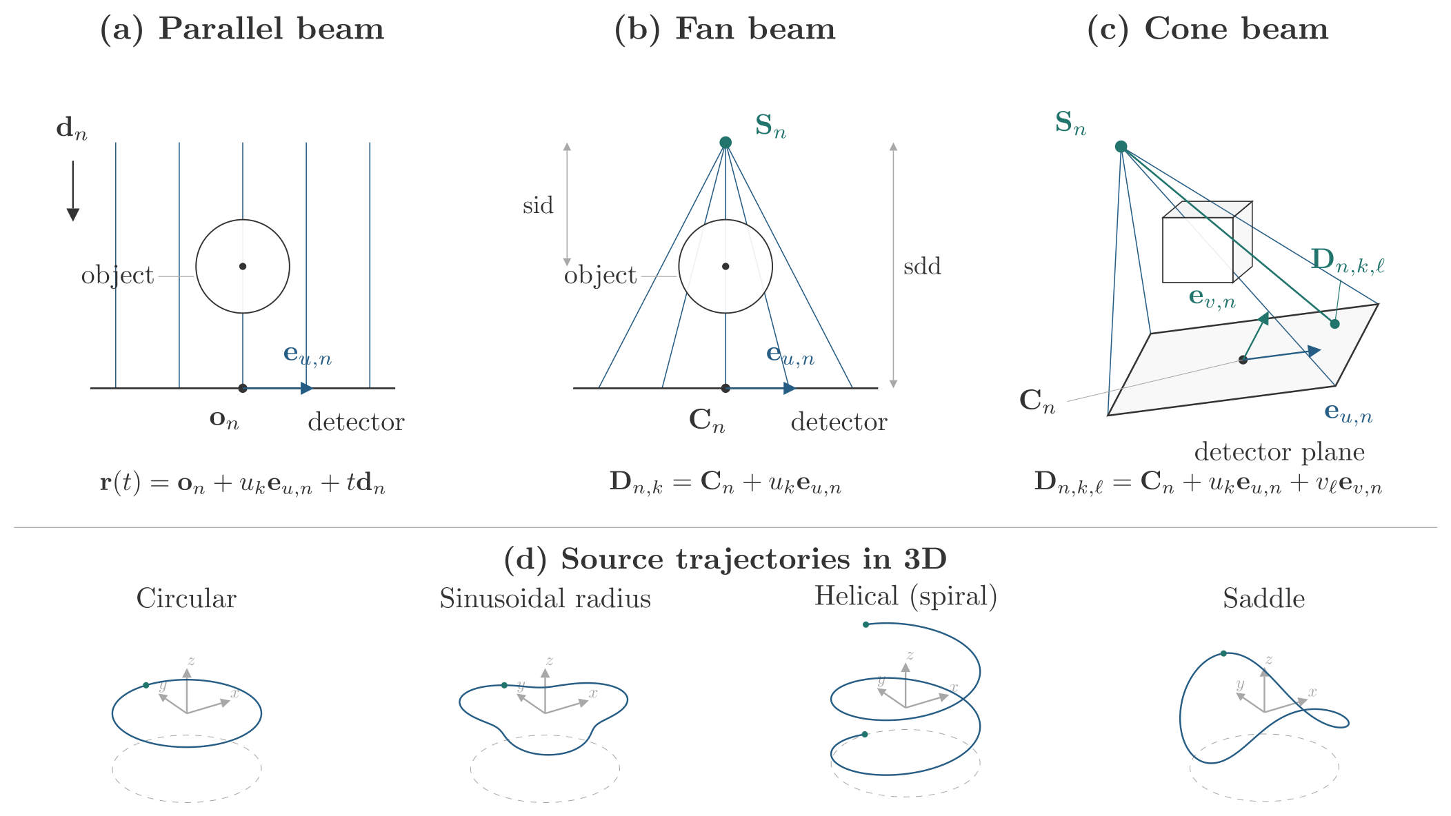
For parallel beams, view n stores $({\mathbf{d}}_n,{\mathbf{o}}_n,{\mathbf{e}}_{u,n})$, each a two-vector. The unit ray direction ${\mathbf{d}}_n$ is orthogonal to the unit detector axis ${\mathbf{e}}_{u,n}$. Pixel k defines the infinite line

$${\mathbf{r}}_{n,k}\left(t\right)={\mathbf{o}}_n+u_k{\mathbf{e}}_{u,n}+t{\mathbf{d}}_n,P_{\mathrm{par}}f(n,k)={\int }_{\mathbb{R}}f\left({\mathbf{r}}_{n,k}\left(t\right)\right)dt.$$

(2)

For fan beams, the tuple is $({\mathbf{S}}_n,{\mathbf{C}}_n,{\mathbf{e}}_{u,n})$. For cone beams, it adds ${\mathbf{e}}_{v,n}$, orthogonal to ${\mathbf{e}}_{u,n}$. The detector point is

$${\mathbf{D}}_{n,k,\mathcal{l}}={\mathbf{C}}_n+u_k{\mathbf{e}}_{u,n}+v_{\mathcal{l}}{\mathbf{e}}_{v,n},L_{n,k,\mathcal{l}}={\parallel {\mathbf{D}}_{n,k,\mathcal{l}}-{\mathbf{S}}_n\parallel }_2.$$

(3)

Omitting the v term gives the fan-beam definition. With $\widehat{\mathbf{d}}=(\mathbf{D}-\mathbf{S})/L$, both divergent-beam projectors integrate the source-to-pixel segment:

$$Pf={\int }_0^{L}f(\mathbf{S}+t\widehat{\mathbf{d}})dt.$$

(4)

The segment is clipped to the volume box before traversal. Rays do not extend through the detector or behind the source, which matters when either endpoint lies inside the volume. Source and detector-pixel coincidences are invalid. The native flat path rejects detectors viewed edge-on from the source. For stable float32 setup, at least one source or detector-center endpoint must lie within ${10}^6$ voxel lengths of the volume center, and both must lie within ${10}^{15}$. Sampled divergent surfaces apply the corresponding checks to source and pixel endpoints; positions must remain finite in float32.

4.3. Circular and Non-Circular Trajectories

A circular cone-beam generator, at angle $\beta$, uses

$$\begin{array}{cc}\hfill \mathbf{S}\left(\beta \right)& =(-\mathrm{sid}\sin \beta ,\mathrm{sid}\cos \beta ,0),\hfill \end{array}$$

(5)

$$\begin{array}{cc}\hfill \mathbf{C}\left(\beta \right)& =\left(\right(\mathrm{sdd}-\mathrm{sid})\sin \beta ,-(\mathrm{sdd}-\mathrm{sid})\cos \beta ,0),\hfill \end{array}$$

(6)

$$\begin{array}{cc}\hfill {\mathbf{e}}_u\left(\beta \right)& =(\cos \beta ,\sin \beta ,0),{\mathbf{e}}_v=(0,0,1).\hfill \end{array}$$

(7)

Here sid and sdd are source-to-isocenter and source-to-detector distances. Removing z gives fan geometry. Parallel geometry instead specifies the ray direction directly. A spiral generator adds a monotone axial offset to source and detector centers; saddle and sinusoidal generators modulate heights or radii. Explicit calibrated arrays need not follow any generator. The 3D random helper generates source positions and corresponding detector frames for stress tests; it does not enforce reconstruction completeness.

Figure 1. Per-view source and detector geometry for parallel, fan and cone beams, with examples of circular and non-circular trajectories. The top row defines the per-view frames and detector points. The bottom row shows circular, sinusoidal-radius, helical and saddle source paths in a common oblique 3D view; axes indicate world coordinates, and markers indicate the path endpoints (coincident for closed paths). Trajectory parameters are illustrative. Detector samples follow the centered convention in Equation (1).

Figure 1. Per-view source and detector geometry for parallel, fan and cone beams, with examples of circular and non-circular trajectories. The top row defines the per-view frames and detector points. The bottom row shows circular, sinusoidal-radius, helical and saddle source paths in a common oblique 3D view; axes indicate world coordinates, and markers indicate the path endpoints (coincident for closed paths). Trajectory parameters are illustrative. Detector samples follow the centered convention in Equation (1).

Projection and iterative inversion can use any valid ray set. Whether that set contains enough information to reconstruct an object is a separate question. The geometry arrays do not impose Tuy–Smith completeness or turn circular FDK into an exact non-circular inverse [6,7].

4.4. Parameterized Detector Surfaces

A local surface sampler returns offsets $(a_u,a_v,a_n)$ for each detector pixel. In cone geometry these map to world points as

$$\mathbf{D}=\mathbf{C}+a_u{\mathbf{e}}_u+a_v{\mathbf{e}}_v+a_n({\mathbf{e}}_u\times {\mathbf{e}}_v).$$

(8)

The normal sign follows the supplied frame. A flat surface has $(a_u,a_v,a_n)=(u,v,0)$. For the circular frame in 5, cylindrical detector offsets of radius r can be written

$$(a_u,a_v,a_n)=\left(r\sin (u/r),v,r\left[\cos \right(u/r)-1]\right).$$

(9)

This cylinder is source-centered only when $r=\mathrm{sdd}$ in the given circular frame. In 2D, $a_v=0$ and the local normal is $(e_{u,y},-e_{u,x})$. Native kernels connect the source to the resulting fan/cone pixel, or pass a parallel ray through it.

The legacy callback receives complete centered physical coordinate grids. The ParameterizedSurface sampler receives centered physical u/v grids restricted to the executing global pixel rectangle, global view indices and explicit parameter snapshots. It generates only the geometry of the executing block. This distinction matters for a per-view surface: constructing all world pixel positions can cost more memory than the projection batch itself. Explicit parameters also let backward reproduce the forward geometry after a caller changes a parameter. The sampler must be pure, mutable geometry must be listed as parameters, and other captured configuration must be immutable. PyTorch differentiates the sampled positions back to those parameters after the native geometry vector–Jacobian product.

Each pixel remains a point sample of a ray. Analytical helpers assume flat detectors. Reusing them on curved measurements requires resampling onto covered rays of a virtual flat detector, with the interpolation error and coverage limitations of that conversion.

5. Siddon Integration and Its Derivatives

5.1. Cell-Constant Discretization

For a ray $\mathbf{o}+t\mathbf{d}$, an axis-q grid face at b is crossed at $t=(b-o_q)/d_q$. After box clipping, ordered crossings $t_0<\dots <t_M$ divide the ray into segments. The kernel advances to the next face and integrates the value of the traversed cell:

$${\left(A_{\mathrm{\Theta }}x\right)}_j={\displaystyle \sum _{m=0}^{M-1}}{x}_{\mathrm{cell}\left(m\right)}(t_{m+1}-t_m)=\sum _i{a}_{ji}\left(\mathrm{\Theta }\right)x_i.$$

(10)

The coefficients are physical chord lengths. This is exact integration of the cell-constant representation, not interpolation of a continuously varying attenuation field. The implementation needs neither a stored sparse system matrix nor sub-cell quadrature [8]. Numerical setup chooses a nearby ray endpoint where possible to reduce cancellation when the source or detector is far from the volume.

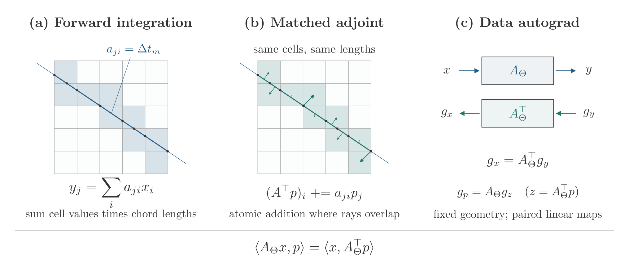
The matched adjoint revisits the same cells and adds $a_{ji}{y}_j$ to each cell. Rays overlap, so these updates use CUDA atomic addition. The defining relation is

$$\langle A_{\mathrm{\Theta }}x,y\rangle =\langle x,A_{\mathrm{\Theta }}^{\top }y\rangle .$$

(11)

It holds for the mathematical discretization; float32 accumulation and different scheduling orders introduce rounding differences. We check these with tolerances rather than requiring bitwise equality.

Figure 2. Forward ray integration and matched atomic-scatter adjoint. Both paths use the same traversed cells and chord lengths. Highlighted cells show a single ray’s nondegenerate face crossings. Forward integration sums cell values times chord lengths; the adjoint scatters a ray value with those same lengths. The data backward pass pairs these kernels; geometry derivatives additionally account for changes in chord lengths.

Figure 2. Forward ray integration and matched atomic-scatter adjoint. Both paths use the same traversed cells and chord lengths. Highlighted cells show a single ray’s nondegenerate face crossings. Forward integration sums cell values times chord lengths; the adjoint scatters a ray value with those same lengths. The data backward pass pairs these kernels; geometry derivatives additionally account for changes in chord lengths.

5.2. Data Autograd and Higher Derivatives

For $y=A_{\mathrm{\Theta }}x$ and $z=A_{\mathrm{\Theta }}^{\top }p$, the reverse-mode data backward rules [21] are

$${\nabla }_x\mathcal{L}=A_{\mathrm{\Theta }}^{\top }{\nabla }_y\mathcal{L},{\nabla }_p\mathcal{L}=A_{\mathrm{\Theta }}{\nabla }_z\mathcal{L}.$$

(12)

For $\mathcal{L}\left(x\right)=\frac{1}{2}{\parallel A_{\mathrm{\Theta }}x-p\parallel }_2^2$, the gradient is $A_{\mathrm{\Theta }}^{\top }(A_{\mathrm{\Theta }}x-p)$ and the fixed-geometry Hessian–vector product is $A_{\mathrm{\Theta }}^{\top }{A}_{\mathrm{\Theta }}v$. The PyTorch wrappers express backward using the paired differentiable operators, allowing derivatives through the data backward itself. This supports unrolled optimization and data-domain second derivatives. It does not establish second derivatives with respect to acquisition geometry.

5.3. First-Order Geometry Derivatives

For a divergent ray with endpoints $a,b$, set $D=b-a$, $L={\parallel D\parallel }_2$ and $\tau \in [0,1]$. Away from changes in crossing order,

$$p=L\sum _m{x}_m({\tau }_{m+1}-{\tau }_m).$$

(13)

At a crossed face $X_q=c$, $\tau =(c-a_q)/D_q$, with derivatives

$${\displaystyle \frac{\partial \tau }{\partial a_q}}={\displaystyle \frac{\tau -1}{D_q}},{\displaystyle \frac{\partial \tau }{\partial b_q}}=-{\displaystyle \frac{\tau }{D_q}}.$$

(14)

Collecting a crossing’s adjacent segments gives a coefficient $x_{\mathrm{before}}-x_{\mathrm{after}}$. Entry and exit use zero outside the volume. Endpoint boundaries fixed at $\tau =0$ or 1 contribute no face-motion derivative. The endpoint gradient combines these face terms with the length derivative:

$$\nabla p=\left[\sum _m{x}_m\mathrm{\Delta }{\tau }_m\right]\nabla L+L\sum _j(x_{\mathrm{before},j}-x_{\mathrm{after},j})\nabla {\tau }_j.$$

(15)

Chain rules then give source, detector-center, detector-axis and surface-parameter derivatives. The parallel-beam kernel handles its line parameterization separately. A geometry derivative of backprojection uses the same bilinear identity: for fixed incoming image gradient g, $\langle g,A_{\mathrm{\Theta }}^{\top }p\rangle =\langle A_{\mathrm{\Theta }}g,p\rangle$.

The cell-constant model is piecewise differentiable in geometry. At a ray through a cell edge or corner, crossings coincide and the kernel returns a derivative from one adjacent side. A central finite difference averages the two sides and can disagree there without indicating a wrong derivative away from the boundary. We consequently use independent double-precision references and nondegenerate rays for gradient comparisons. Geometry second derivatives are rejected because the implemented first-order rule does not define that higher-order contract.

6. Analytical Reconstruction and Learnable Stages

6.1. Composition and Physical Isocenter

FBP and FDK consist of projection weighting, detector-u filtering, angular quadrature and voxel-driven interpolation. Unlike the matched adjoint, the analytical gather samples filtered projections at a voxel’s projected detector coordinate and applies magnification weights. Let ${\mathbf{n}}_n$ be the detector normal oriented from source to detector and $\mathbf{c}$ the physical isocenter. Define

$${\mathrm{sdd}}_n=({\mathbf{C}}_n-{\mathbf{S}}_n)·{\mathbf{n}}_n,{\mathrm{sid}}_n=(\mathbf{c}-{\mathbf{S}}_n)·{\mathbf{n}}_n,U_n\left(\mathbf{x}\right)=(\mathbf{x}-{\mathbf{S}}_n)·{\mathbf{n}}_n.$$

(16)

Using $-{\mathbf{S}}_n$ in place of $\mathbf{c}-{\mathbf{S}}_n$ would bind the amplitude to the coordinate origin. The implementation fits source lines along detector normals in least squares and rejects a rank-deficient fit. An explicit physical isocenter is required when this inference is ambiguous, including a single view. For non-circular geometry, supplying the intended physical isocenter is recommended; inference does not require a circular orbit.

The source-to-voxel line meets the detector plane at

$${\mathbf{H}}_n\left(\mathbf{x}\right)={\mathbf{S}}_n+{\displaystyle \frac{{\mathrm{sdd}}_n}{U_n\left(\mathbf{x}\right)}}(\mathbf{x}-{\mathbf{S}}_n),u_n=({\mathbf{H}}_n-{\mathbf{C}}_n)·{\mathbf{e}}_{u,n},v_n=({\mathbf{H}}_n-{\mathbf{C}}_n)·{\mathbf{e}}_{v,n}.$$

(17)

For a flat detector normal to the central ray, the cosine weights are

$$w_{\cos }^{\mathrm{fan}}\left(u\right)={\displaystyle \frac{\mathrm{sdd}}{\sqrt{{\mathrm{sdd}}^2+u^2}}},w_{\cos }^{\mathrm{cone}}(u,v)={\displaystyle \frac{\mathrm{sdd}}{\sqrt{{\mathrm{sdd}}^2+u^2+v^2}}}.$$

(18)

The complete pipeline accounts for detector offsets in these distances. More general fixed geometry can supply its own projection-weight tensor.

6.2. Finite Discrete Ramp and Quadrature

The ramp uses a finite sampled Ram–Lak impulse response in the angular-frequency convention [2]:

$$h\left[0\right]={\displaystyle \frac{\pi }{2}},h\left[k\right]=\left\{\begin{array}{cc}-2/\left(\pi k^2\right),\hfill & k\mathrm{odd},\hfill \\ 0,\hfill & k\ne 0\mathrm{even}.\hfill \end{array}\right.$$

(19)

For padded length M, wrapped signed lags define the symmetric kernel. If $H_M$ is its discrete Fourier response and W an apodization window, the filtered samples are

$$q={\displaystyle \frac{1}{\mathrm{\Delta }u}}\mathrm{crop}\left[{\mathcal{F}}_M^{-1}\left\{H_{M}W{\mathcal{F}}_M\left[\mathrm{pad}\left(p_w\right)\right]\right\}\right].$$

(20)

The spacing factor occurs once. With the unwindowed response, padding to at least twice the detector width gives linear convolution on the retained samples. Directly sampling $\left|\omega \right|$ instead gives a different finite filter, including different DC behavior. The finite impulse retains a small positive DC response; forcing it to zero changes the low-frequency reconstruction bias.

Writing $\nu =2\left|f\right|$ for normalized sample frequency, the available windows are 1 (Ram–Lak), $(1+\cos \pi \nu )/2$ (Hann), $0.54+0.46\cos \pi \nu$ (Hamming), $\cos (\pi \nu /2)$ (cosine), and $\sin (\pi \nu /2)/(\pi \nu /2)$ (Shepp–Logan, with the limit at zero). Windowing changes the noise–resolution tradeoff rather than the ray model.

Open angle lists use trapezoidal weights

$$\mathrm{\Delta }{\beta }_1={\displaystyle \frac{{\beta }_2-{\beta }_1}{2}},\mathrm{\Delta }{\beta }_n={\displaystyle \frac{{\beta }_{n+1}-{\beta }_{n-1}}{2}},\mathrm{\Delta }{\beta }_N={\displaystyle \frac{{\beta }_N-{\beta }_{N-1}}{2}}.$$

(21)

Periodic scans close the angular interval. Full-turn fan/cone weights include a half-redundancy factor; a uniform full turn therefore integrates to $\pi$. Parker weighting handles circular short-scan redundancy before filtering, with the acquisition span controlling the smooth end windows [4]. Parker and quadrature share the same periodic-scan classification. Different decisions near a full turn would apply short-scan weights and the full-turn half factor together, reducing the amplitude twice. The public short-scan path checks the circular orbit, angle order and span, detector-u orientation, and constant detector distance and offset.

For a circular scan with retained angular span B, set $\delta =\max ({\gamma }_{\max },(B-\pi )/2)$ and $\gamma =\arctan (u/\mathrm{sdd})$. After shifting the first angle to zero, the generalized Parker taper is

$$w_P(\beta ,\gamma )=\left\{\begin{array}{cc}{\sin }^2\left({\displaystyle \frac{\pi \beta }{4(\delta -\gamma )}}\right),\hfill & 0\le \beta <2(\delta -\gamma ),\hfill \\ 1,\hfill & 2(\delta -\gamma )\le \beta \le \pi -2\gamma ,\hfill \\ {\sin }^2\left({\displaystyle \frac{\pi (\pi +2\delta -\beta )}{4(\delta +\gamma )}}\right),\hfill & \pi -2\gamma <\beta \le \pi +2\delta ,\hfill \\ 0,\hfill & \mathrm{otherwise}.\hfill \end{array}\right.$$

(22)

At the minimum short scan, $\delta ={\gamma }_{\max }$. For a longer valid short scan the acquired span broadens the tapers. Degenerate endpoint limits are guarded numerically. Full circular scans use unit Parker weights; their half-redundancy factor belongs in the angular quadrature.

6.3. Weighted Gathers and Their Transposes

Let ${\tilde{q}}_n$ denote interpolation of filtered data that already include angular weights. Parallel FBP uses the projected coordinate $u_n=(\mathbf{x}-{\mathbf{o}}_n)·{\mathbf{e}}_{u,n}$ and returns

$$B_{\mathrm{par}}q\left(\mathbf{x}\right)={\displaystyle \frac{1}{2\pi }}\sum _n{\tilde{q}}_n\left(u_n\right).$$

(23)

Fan FBP and cone FDK use

$$Bq\left(\mathbf{x}\right)={\displaystyle \frac{\overline{\mathrm{sdd}}}{2\pi \overline{\mathrm{sid}}}}\sum _n{\left({\displaystyle \frac{{\mathrm{sid}}_n}{U_n\left(\mathbf{x}\right)}}\right)}^2{\tilde{q}}_n(u_n\left(\mathbf{x}\right),v_n\left(\mathbf{x}\right)),$$

(24)

with the v coordinate omitted for fan beams. The overline is a mean over views. Linear interpolation is used in 2D and bilinear interpolation on the cone detector. Both detector axes need at least two bins. Cone FDK filters along u, never along v. The mean-distance scale reduces to $\mathrm{sdd}/\left(2\pi \mathrm{sid}\right)$ for a circular orbit; the non-circular extension remains an approximation.

For fixed geometry, the gather is a discrete linear map B. Its data gradient is $B^{\top }g$, implemented by scattering the same interpolation coefficients, distance weights and scale. Substituting the Siddon projector A would give a different derivative because $B\ne A^{\top }$. Ordinary PyTorch autograd differentiates cosine weights, FFT filtering, angular weights and explicit replacement tensors. The complete fbp and fdk functions expose projection_weights, angular_weights and filter_response; a replacement frequency response is the full real-rFFT multiplier in physical units, not an additional window. These APIs return signed float32 CUDA reconstructions. Nonnegative clamping is a caller choice.

6.4. Slice-Windowed Helical Approximation

For an axial helix, source height and unwrapped angle determine a center angle ${\beta }_c\left(z\right)$ for each reconstructed slice. helical_view_weights integrates angular sample cells over $[{\beta }_c\left(z\right)-\pi ,{\beta }_c\left(z\right)+\pi ]$, clips the boundary cells fractionally, and includes the half-redundancy factor:

$$w_n\left(z\right)={\displaystyle \frac{1}{2}}\left|I_n\cap [{\beta }_c\left(z\right)-\pi ,{\beta }_c\left(z\right)+\pi ]\right|,\sum _n{w}_n\left(z\right)=\pi .$$

(25)

Here $I_n$ is the angular cell around view n. Angles, slice centers and interval arithmetic use double precision internally. The default weight generator rejects missing full-turn coverage rather than renormalizing it. Filtering is performed once; each slice then uses its own weights in the native cone analytical gather. Explicit replacement slice weights remain differentiable and replace the entire window and quadrature stage. Supplied weights bypass the default full-turn coverage check and are neither normalized nor clamped; the caller is responsible for their coverage and scale. The supplied angles must still match the axial helix and remain strictly monotone.

This is a slice-windowed FDK approximation on native cone data, not exact helical inversion. It does not implement cone-parallel rebinning or conjugate-ray 3D weights. The path requires an axial helix with radial detector normals, and detector truncation is still possible even with complete angular windows. One launch per slice avoids a view-by-volume weight tensor but adds launch overhead. Like the other analytical APIs, it does not inherit the native projector’s curved, streamed or distributed execution.

7. Execution, Memory and Distributed Ownership

7.1. PyTorch and Numba

PyTorch owns tensors and autograd state; Numba compiles and launches the CUDA traversal, scatter and analytical kernels [3,22]. CUDA tensor views expose the same device memory to Numba, avoiding a second tensor allocation for kernel access. External stream handles connect launches to the caller’s PyTorch stream. Events protect geometry reuse, buffer reuse and transfers across streams. Selecting the input’s CUDA context matters when an operation runs on a device different from the process’s current device.

Native cone traversal uses internal layouts suited to kernel access, while the public volume and sinogram axes remain those in Section 4. The execution planner accounts for layout copies as well as nominal inputs. Atomic-scatter accumulation explains why correct runs with different execution orders may disagree in their final float32 bits.

7.2. Spatial, View and Detector Blocks

Let disjoint spatial tiles select columns of A and view/pixel blocks select rows. With $C_t$ inserting local tile t into the global volume and $R_b$ selecting ray block b, define $A_{bt}=R_{b}A{C}_t$. Then

$${\left(Ax\right)}_b=\sum _t{A}_{bt}{x}_t,{\left(A^{\top }y\right)}_t=\sum _b{A}_{bt}^{\top }{y}_b.$$

(26)

Tiles retain global voxel coordinates, including incomplete edge tiles. These equations explain both how a volume too large for one GPU can be processed and why local partial results must be summed. Cutting a ray into disjoint cell groups preserves its cell-constant integral; rounding changes with the addition order.

Projection can traverse space while retaining partial ray batches. Backprojection benefits from retaining a spatial tile’s GPU accumulator across all contributing view and pixel batches, then downloading it once. Returning every partial volume to the CPU would repeat transfers and host additions. The planner compares operation-specific orders and slab/block shapes using short pilots on one representative CUDA device after a warmup launch. It divides each measured prefix’s elapsed time by its measured launch count and multiplies by the full native launch count to estimate elapsed time. The smallest estimate is selected, with estimated host-to-device plus device-to-host bytes breaking ties. It does not assume that a good projection schedule is also good for backprojection.

CPU inputs always use streamed CUDA work. A CUDA input can use the full-volume path when a conservative additional working set fits; otherwise it streams. View, spatial and detector limits can force a particular decomposition. Pinned slots bound host staging, and separate transfer streams with events allow upload, compute and download to overlap without reusing an unfinished buffer. Capacity admission checks total live buffer bytes, estimated allocator reservation bytes, the largest individual allocation and host geometry workspace separately. The inventory includes geometry, VJP buffers, layout copies, collective staging and cached slots. If the minimum tile/view/pixel batch cannot satisfy these constraints after reducing automatic dimensions, planning raises an error; explicit limits must be reduced by the caller. Available GPU memory is an observation rather than a reservation; allocator fragmentation and concurrent allocations can still prevent a plan from fitting.

The schedule argument accepts auto, spatial, views and window. The last requests a bounded two-tile window; capacity can require a serial spatial fallback. After an instrumented streamed call, last_execution_stats records actual copy payloads, native launches and layouts, planned capacity, and pilot metadata. Pilot estimates describe schedule selection, not a measured full-workload time. This attribute is None before execution, after errors and on the uninstrumented full-CUDA path.

Tensor streaming reduces GPU residency, but the complete tensors and their autograd gradients still occupy the input device. To exceed host RAM as well, the caller must use block stores and keep solver state blockwise. This is the purpose of TensorStore, mapped NpyStore arrays and project_into/backproject_into. These numerical methods overwrite caller-owned float32 blocks and return the output store without creating an autograd graph. Known aliases and read-only outputs are rejected before writes; a custom store must enforce its own hidden alias constraints.

7.3. View Partitions

One-process multi-GPU execution divides views, launches nonempty shards on several devices and gathers the complete sinogram. Distributed view mode instead retains each rank’s sinogram shard and replicates the volume. For rank r, write $A_r=R_{r}A$. Projection returns $A_{r}x$, and backprojection uses a SUM reduction:

$$A^{\top }y=\sum _r{A}_r^{\top }{y}_r.$$

(27)

A global least-squares loss is ${\sum }_r\frac{1}{2}{\parallel A_{r}x-y_r\parallel }^2$. Each rank supplies its local sum, and native backward sums data and geometry contributions. Using a local mean without accounting for shard sizes would change the global objective when views are unevenly divided.

Conversely, backprojection output is replicated. A loss applied identically to that output on every rank must be divided by the number of ranks. An additional DDP reduction on native image gradients would reduce them a second time. All ranks must make the same collective calls, including ranks with empty view shards. These rules concern mathematical multiplicity, not only launch syntax.

7.4. Spatial Partitions and Disk CGLS

In spatial mode, rank r owns a fixed volume slab, $A_r=A{C}_r$. The constructor receives the global shape, retained as global_volume_shape. Each rank’s volume_slice maps its slab into that global array; volume_shape and local_volume_shape give the required local tensor shape. Empty slabs are valid, and global physical coordinates are preserved. Ray data and projection_shape are replicated, and forward contributions are summed:

$$Ax=\sum _r{A}_r{x}_r,{\left(A^{\top }y\right)}_r=A_r^{\top }y.$$

(28)

The returned backprojection is local to the owned slab. A replicated projection loss is divided by the number of ranks; a loss on owned backprojection cells is summed. Norms must also respect ownership: sum disjoint volume norms across ranks but count a replicated ray vector once.

Starting from $x=0$, CGLS initializes $r=y$, $s=A^{\top }r$ and $p=s$. The disk CGLS example keeps the volume estimate x, image gradient s, search direction p, residual r and projected direction q in block stores. With $s=A^{\top }r$, one iteration is

$$\begin{array}{cccc}\hfill q& =Ap,\hfill & \hfill \alpha & ={\displaystyle \frac{\langle s,s\rangle }{\langle q,q\rangle }},\hfill \end{array}$$

(29)

$$\begin{array}{cccc}\hfill x& \leftarrow x+\alpha p,\hfill & \hfill r& \leftarrow r-\alpha q,\hfill \end{array}$$

(30)

$$\begin{array}{cccc}\hfill s^{\prime }& =A^{\top }r,\hfill & \hfill \gamma & ={\displaystyle \frac{\langle s^{\prime },s^{\prime }\rangle }{\langle s,s\rangle }},p\leftarrow s^{\prime }+\gamma p.\hfill \end{array}$$

(31)

The example uses CGLS, a conjugate-gradient method for the least-squares problem [18]. Inner products accumulate float64 block sums; state updates use float32. The complete q must remain available until the global $\alpha$ is known. Reconstructing it per residual block or discarding it before the norm decision would change the algorithm or add work. Completed-iteration checkpoints store rank-local ownership rather than gathering the full volume. Resume validates partition, ownership, shapes, dtype and scan metadata, then restores the solver state; the requested iteration count is a total target including completed iterations. These metadata do not fingerprint the complete geometry or measurement arrays, which must be supplied unchanged by the caller.

The tensor CGLS example admits all five states $x,s,p,r,q$ together with native pipeline and scratch buffers before allocating them on CUDA. If that working set exceeds the capacity constraints, ranks agree to keep solver state on CPU and execute the native operators through streaming. This solver decision is separate from an individual projector call’s admission check; the recorded scaling experiment below retains CUDA state. The disk solver instead keeps vector operations and norm temporaries blockwise. Boundary-coupled regularizers on spatial partitions require caller-managed halo exchange; the supplied SIRT and TV tensor examples do not implement distributed spatial regularization. Tensor autograd and a disk numerical solver are separate interfaces because the latter must bound every vector operation, not just A and $A^{\top }$.

8. Experiments and Numerical Evidence

8.1. Data, Hardware and Metric Definitions

Experiments use synthetic Shepp–Logan phantoms [23] and measured cone-beam projections of a walnut [24]. The new 2.2.1 reconstruction examples use one node with one NVIDIA GeForce RTX 4070 SUPER. The recorded 2.2.0 scaling experiment uses NVIDIA A100-SXM-64GB GPUs in three configurations: one node with one GPU, one node with four GPUs, and two nodes with eight GPUs.

For synthetic references with peak attenuation 1, $\mathrm{PSNR}=10{\log }_{10}(1/\mathrm{MSE})$, where MSE averages over all reconstructed voxels. A Gaussian projection-noise level of 1% means standard deviation equal to 1% of the largest noiseless projection, not 1% voxel noise. Relative data error is $\parallel u-u_{\mathrm{ref}}{\parallel }_2/{\parallel u_{\mathrm{ref}}\parallel }_2$. Speedup divides the one-GPU median by the corresponding multi-GPU median for the same workload. Ground-truth PSNR is not assigned to the measured walnut, for which no independent reference volume is supplied.

8.2. Measured Walnut Reconstruction

The public dataset contains 721 projections acquired at 0.5-degree steps, with source-to-isocenter distance 210.66 mm, source-to-detector distance 553.74 mm and detector pitch 0.050 mm [24]. The distributed derivative corrects the offset rotation axis, bins detector pixels by eight, crops to $256\times 256$, keeps every third view, estimates an air level per projection, and computes $-\log (I/I_0)$. The stored 241 views include a repeated full-turn endpoint; reconstruction removes it and uses 240 distinct views. This preprocessing is part of the data interpretation, not a simulated scan.

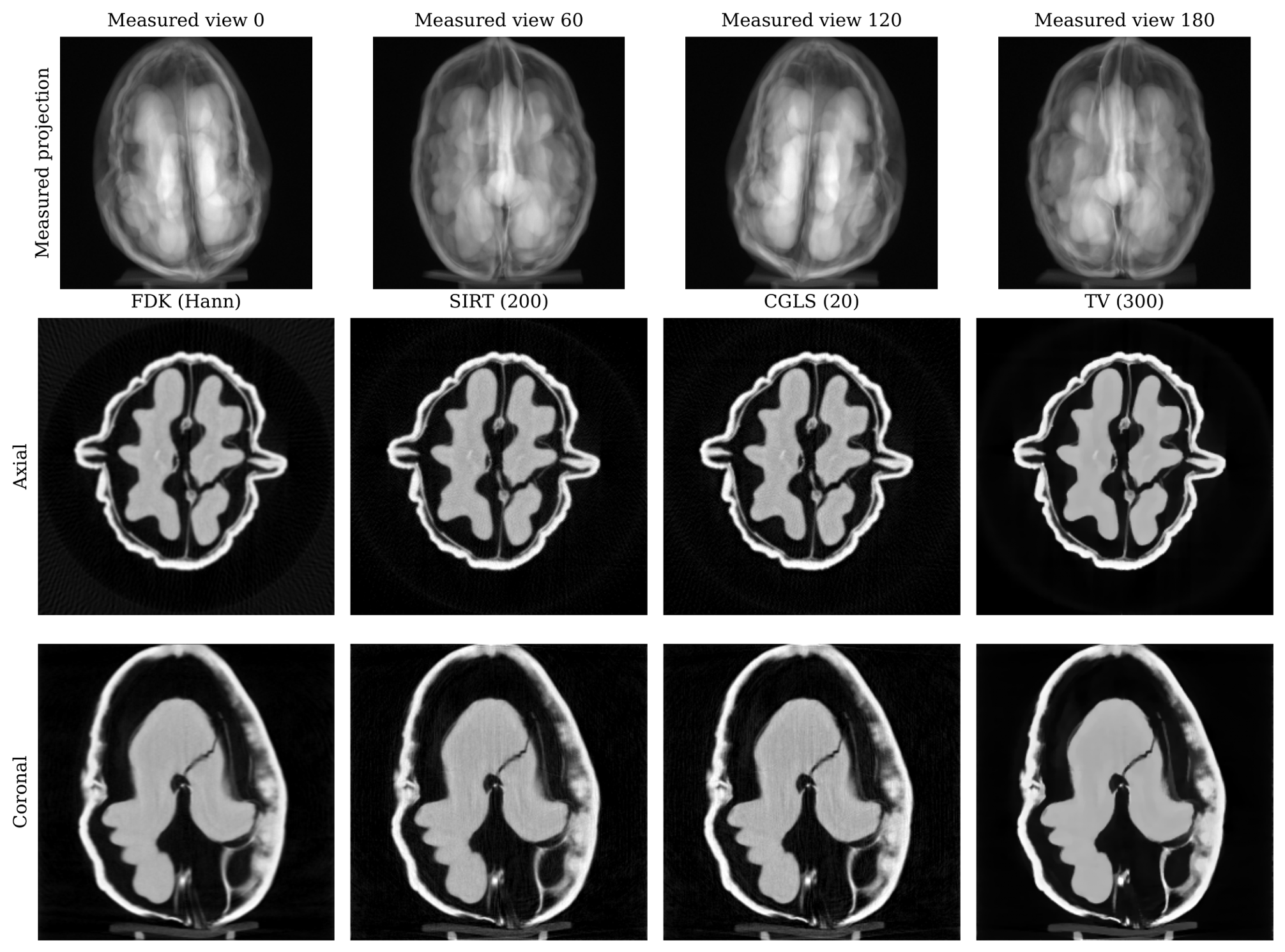
fig:walnut shows saved ${256}^3$ reconstructions of these measured data. FDK uses a Hann window; SIRT uses 200 iterations, CGLS 20, and nonnegative TV-regularized least squares 300 Adam steps with weight 0.3. The display scale is based on the FDK shell’s 99.95th percentile and is shared with the iterative target. Images use the same $[0,1]$ display range, rather than being independently normalized. The saved panels support a visual comparison; they do not establish a ranking against ground truth. A separate 2.2.1 run at ${128}^3$ repeats the measured-data pipeline on the single-GPU configuration above.

Figure 3. Measured walnut cone-beam data. Top: four measured projection views, transposed into detector-v rows and detector-u columns, in the stored acquisition-row display order (row zero at the top). Bottom: axial and coronal central slices of FDK, SIRT, CGLS and TV reconstructions at ${256}^3$ using all 240 distinct views. The projection and reconstruction display ranges are separate; all reconstruction panels share $[0,1]$. These saved public example assets were retrieved at source revision 4ac2e15; they are distinct from the synthetic helical experiment. Data: Meaney (2022), CC BY 4.0 [24].

Figure 3. Measured walnut cone-beam data. Top: four measured projection views, transposed into detector-v rows and detector-u columns, in the stored acquisition-row display order (row zero at the top). Bottom: axial and coronal central slices of FDK, SIRT, CGLS and TV reconstructions at ${256}^3$ using all 240 distinct views. The projection and reconstruction display ranges are separate; all reconstruction panels share $[0,1]$. These saved public example assets were retrieved at source revision 4ac2e15; they are distinct from the synthetic helical experiment. Data: Meaney (2022), CC BY 4.0 [24].

8.3. Synthetic Iterative Reconstruction

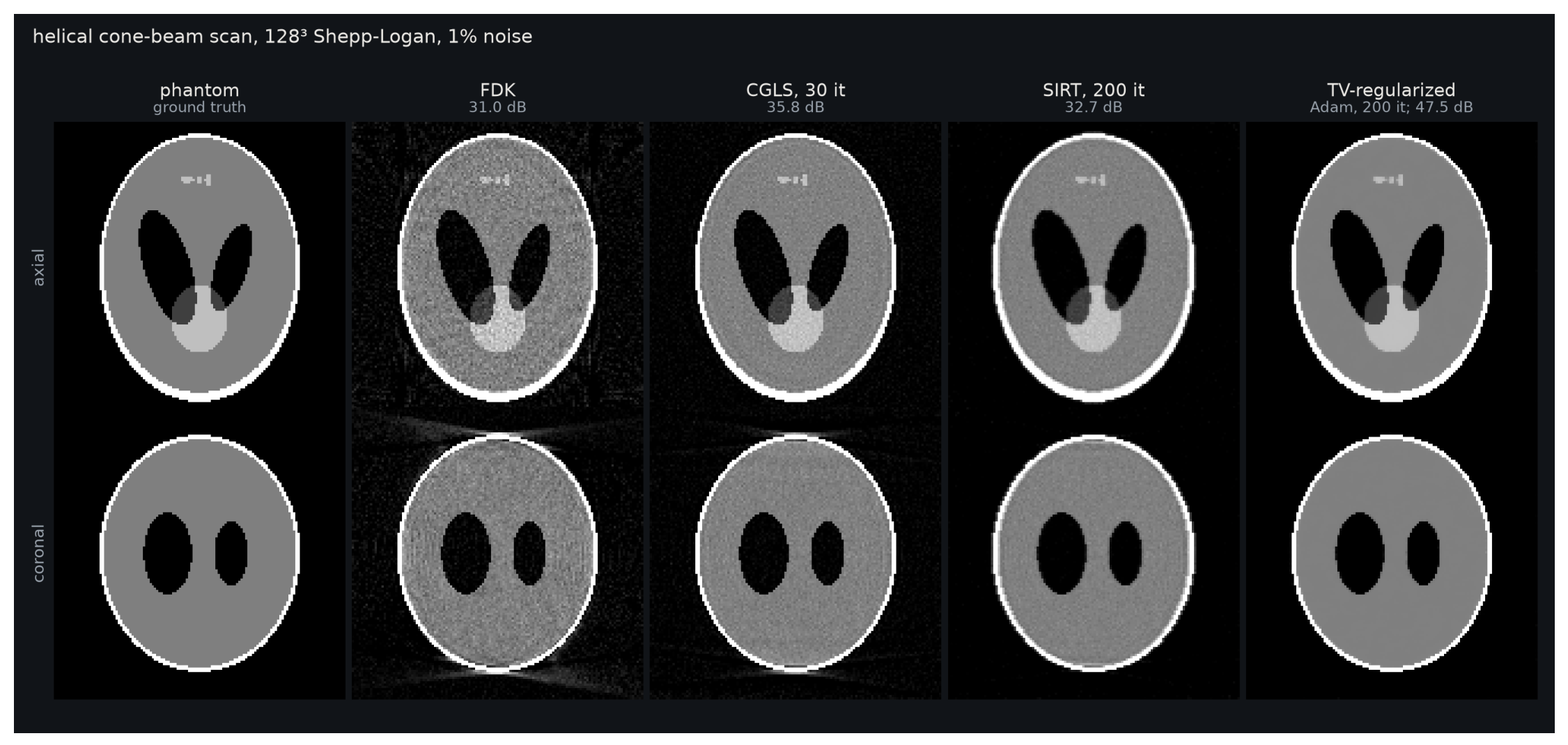
The new 2.2.1 experiment uses a ${128}^3$ Shepp–Logan phantom, 360 helical cone views, detector shape $(384,256)$, detector pitch 0.8, and 1% Gaussian projection noise. The source-to-isocenter and source-to-detector distances are 320 and 512 in voxel-length units, with a 38.4-unit axial span over one turn. CGLS runs for 30 iterations, nonnegative SIRT for 200, and TV-regularized nonnegative least squares for 200 Adam steps with TV weight 1. The example FDK wrapper applies clamp_min(0) before the reported synthetic PSNR is computed.

SIRT starts from $x^{\left(0\right)}=0$ and applies

$$x^{(k+1)}=\max \left(0,x^{\left(k\right)}+C{A}^{\top }R(y-A{x}^{\left(k\right)})\right).$$

(32)

Here R and C are diagonal, with entries $R_{jj}=1/{\left(A\mathbf{1}\right)}_j$ and $C_{ii}=1/{\left(A^{\top }\mathbf{1}\right)}_i$ where the respective denominator is positive, and zero otherwise. R normalizes each ray residual by its total intersected length; C normalizes the backprojected update by accumulated voxel sensitivity. The maximum enforces nonnegativity componentwise.

The TV data term is half the mean squared ray residual. The implemented regularizer is

$$\mathrm{TV}\left(x\right)={\displaystyle \frac{1}{\left|\mathrm{\Omega }\right|}}\sum _{i\in \mathrm{\Omega }}\sqrt{d_x{\left(i\right)}^2+d_y{\left(i\right)}^2+d_z{\left(i\right)}^2+{10}^{-6}},$$

(33)

where $d_x\left(i\right)$, $d_y\left(i\right)$ and $d_z\left(i\right)$ are forward one-voxel differences from the same voxel i on the shared cropped domain $\mathrm{\Omega }=\{0,\dots ,D-2\}\times \{0,\dots ,H-2\}\times \{0,\dots ,W-2\}$. These differences are not divided by voxel spacing. Each Adam update [25] is followed by projection onto nonnegative voxel values. Averaging the data and TV terms removes direct scaling with ray and voxel counts, but the TV weight still depends on geometry, resolution, voxel spacing and data scale.

Figure 4. New 2.2.1 helical Shepp–Logan reconstruction with 1% Gaussian projection noise at ${128}^3$. Labels give PSNR against the synthetic volume. FDK is the trajectory-array approximate baseline; CGLS, SIRT and TV use the native matched operators. This experiment uses simulated measurements, not measured walnut projections.

Figure 4. New 2.2.1 helical Shepp–Logan reconstruction with 1% Gaussian projection noise at ${128}^3$. Labels give PSNR against the synthetic volume. FDK is the trajectory-array approximate baseline; CGLS, SIRT and TV use the native matched operators. This experiment uses simulated measurements, not measured walnut projections.

8.4. Calibration and Analytical Learning

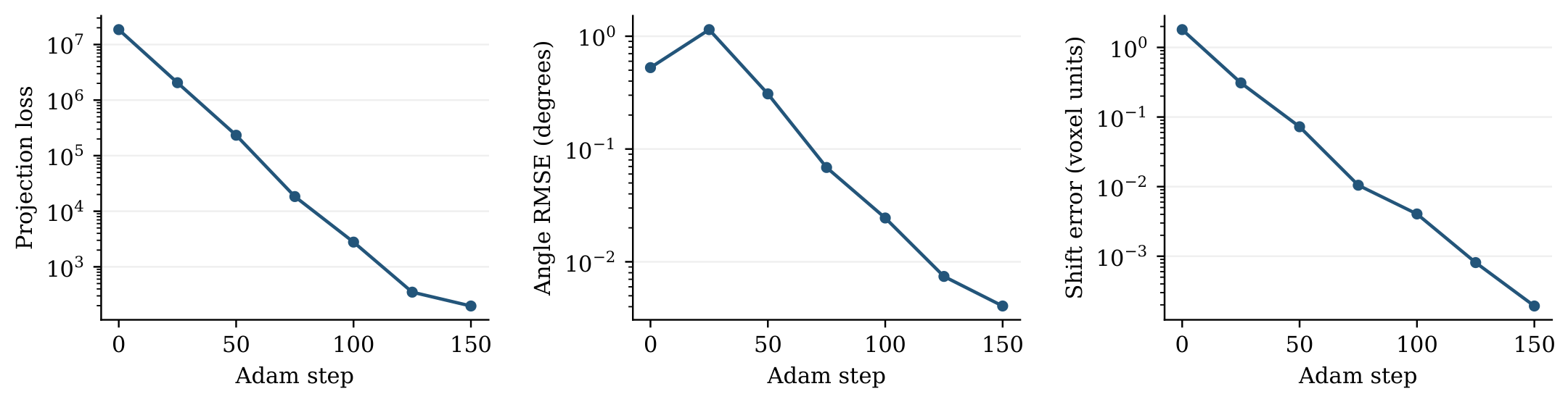
fig:calibration plots the seven samples of a new 2.2.1 synthetic ${64}^3$, 360-view calibration run on one RTX 4070 SUPER and one node. It optimizes per-view angles and a shared detector shift. Across 150 Adam steps, angular RMSE changes from 0.52690 to 0.004058 degrees and detector-shift error from 1.80278 to 0.000193 voxel-length units. At step 25 the projection loss has decreased while angular RMSE has risen to 1.14469 degrees. Reporting both prevents a lower data residual from being mistaken for accurate geometry at every iteration. Samples were captured every 25 steps, including the initial and final states. The initial per-view angle perturbations use seed 7 and nominal standard deviation 0.5 degrees; the true shared detector shift is $(1.5,-1.0)$. Adam learning rates are ${10}^{-3}$ for angles and $5\times {10}^{-2}$ for shifts.

Figure 5. New synthetic geometry-calibration samples: projection loss, angular RMSE and detector-shift error. Only the seven recorded samples are marked and connected. Angles and shifts are calibrated variables; this is distinct from learning analytical weights at fixed geometry.

Figure 5. New synthetic geometry-calibration samples: projection loss, angular RMSE and detector-shift error. Only the seven recorded samples are marked and connected. Angles and shifts are calibrated variables; this is distinct from learning analytical weights at fixed geometry.

The new fixed-geometry learning experiments instead optimize a frequency-response gain and detector weights for 20 Adam steps on one noisy synthetic sample, with 180 views and seed 7. Table 2 reports before/after PSNR. The manual composed pipeline and complete public API agree exactly at the printed precision for each beam. These are training-sample fits demonstrating gradient flow through filtering and analytical gathers; they do not measure generalization to another phantom or noise realization.

The new ${32}^3$ helical-FDK example uses 720 views over four turns, a $96\times 96$ detector, pitch 0.8, sid 128 and sdd 204.8, with a 64-unit source-height range. It obtains 32.99 dB. Manual composition and helical_fdk differ by at most $3.58\times {10}^{-7}$, and each slice’s angular weights sum to 3.141593. These observations check composition and coverage; they do not prove exact helical inversion.

8.5. Distributed Scaling at ${512}^3$

The recorded 2.2.0 benchmark uses a circular ${512}^3$ Shepp–Logan volume, 360 views, detector shape $(1024,768)$, detector pitch 1.25, voxel spacing 1, sid 1280 and sdd 2048. Solver state is float32 on CUDA; CGLS norms accumulate in float64. The distributed partition is by views. No GPU allocator cap is imposed.

For projection and adjoint, three warmups precede seven synchronized wall-time samples. Distributed samples use the slowest rank’s elapsed time, with the rank-maximum reduction outside the timed region. The reported statistic is the median. CGLS first warms up for two iterations, then measures three separate ten-iteration solves. Each solve includes initialization; its elapsed time is divided by ten. Thus the CGLS column is an amortized solve cost, not an isolated steady-state iteration.

Figure 6. Speedup calculated from the medians in Table 3. The adjoint and CGLS scale less than projection for this workload. Dashed lines indicate ideal speedup at each GPU count, not an empirical fit. Raw repeated timing samples accompany the source package.

Figure 6. Speedup calculated from the medians in Table 3. The adjoint and CGLS scale less than projection for this workload. Dashed lines indicate ideal speedup at each GPU count, not an empirical fit. Raw repeated timing samples accompany the source package.

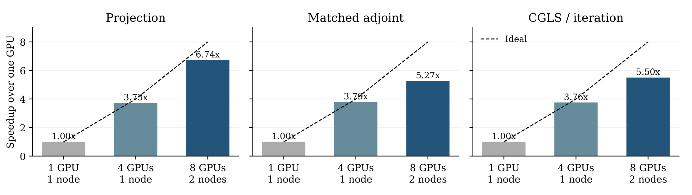
All ranks pass the benchmark’s numerical checks. Across the multi-GPU configurations, relative L2 disagreement with the single-GPU reference is zero for projection, at most $4.15\times {10}^{-7}$ for the adjoint, and at most $4.46\times {10}^{-7}$ for CGLS. Normalized adjoint inner-product error is below $3.0\times {10}^{-8}$. Ten iterations produce a relative residual of about 0.04349 and PSNR 24.93 dB on every configuration. This workload is larger than the ${128}^3$ quality experiment and uses fewer CGLS iterations, so their PSNR values should not be compared as a scaling effect.

The eight-GPU experiment is a two-node run. It establishes cross-node operation for the recorded view-partition workload, not a universal speedup for small arrays or a performance result for spatial partitions, disk stores, geometry learning or analytical FDK. The benchmark records correctness and speed together because a fast distributed computation with a missing reduction would be invalid.

8.6. Numerical Regressions and Validation Boundaries

An independent float64 ray/box reference checks chord lengths rather than reproducing the CUDA traversal. Adjoint tests compare inner products and finite differences check data and geometry derivatives. Execution tests cover nondefault streams, uneven/empty view shards, spatial tails, tiled detector coordinates, parameter mutation and numerical store ownership. A local 2.2.1 run on one RTX 4070 SUPER passed 254 tests in the reconstruction API, analytical autograd, weighting, filter-window and adjoint-inner-product subset. Bounded formal checks address partition and ownership protocols; they complement CUDA runs and do not constitute a proof for arbitrary array sizes or runtime interleavings.

Recorded single-GPU analytical regressions expose why amplitude and quality need separate metrics. Holding the corrected finite ramp fixed, a 330-degree disk scan’s center amplitude changes from 1.830670 to 0.999931 after correcting Parker weighting; a 350-degree scan changes from 1.941608 to 0.999931. A 359.92093-degree, 7200-view scan with its endpoint included changes from 0.499966 to 0.999974 when Parker and quadrature share scan classification. Translating fan and cone geometry changes a former amplitude ratio of 1.125000 to 1.000000 after using the physical isocenter. These are saved regression measurements on one RTX 4070 SUPER, not new distributed benchmarks.

Raw RMSE improves in all three cases in Table 4, whereas clamped PSNR does not. The old negative bias was partly hidden by clamping. We therefore do not infer that corrected amplitude resolves aliasing or edge-resolution artifacts. Likewise, the Gaussian-filter regression compares filtered projections with a continuous Fourier integral; its RMSE reduction from $3.77992\times {10}^{-3}$ to $2.66667\times {10}^{-8}$ is not an image-reconstruction metric.

9. Discussion and Limits

The common ray model lets a change of trajectory, detector surface or execution partition reuse the same definition of A and $A^{\top }$. Geometry differentiation then follows movement of the segment boundaries rather than treating calibration as an image-only problem. Analytical reconstruction follows a separate path because its interpolation and distance weighting define a different linear operator, whose transpose is required when filter or detector weights are learned.

The model has specific limits. Cell-constant point-ray sampling does not integrate a pixel footprint and is only piecewise differentiable in geometry. Voxel spacing is isotropic. FDK is approximate away from its favorable circular setting, and the helical extension remains a slice-windowed approximation with coverage and truncation constraints. Analytical geometry gradients, curved detectors and streamed/distributed analytical execution are outside the current analytical contract. These limits guide the choice between native iterative reconstruction and the analytical APIs.

Memory modes also require a choice. View partitions replicate volume state; spatial partitions distribute it but replicate ray batches. Tensor streaming bounds CUDA residency without removing full host tensors or autograd state. Disk numerical operations address that remaining capacity limit only when the solver’s norms, updates and checkpoints also operate on blocks. Automatic planning balances measured execution and transfer estimates; it cannot guarantee allocation under arbitrary fragmentation or performance on a different workload.

The experiments cover real projection data, controlled synthetic references, training-sample analytical learning and a recorded cross-node scaling workload. They provide neither a clinical evaluation nor an inter-library performance ranking. A saved visual walnut comparison has no ground-truth PSNR, and a learned filter fitted to one noisy phantom is not evidence of generalization. Performance claims are tied to the reported volume, detector, view count, partition and software release.

10. Conclusion

diffct 2.2.1 provides per-view CT geometry, cell-constant Siddon projection and a matched adjoint, first-order geometry and surface derivatives, and differentiable analytical reconstruction with its own discrete transpose. Spatial, view and pixel blocks preserve the native model while extending its execution to several GPUs and to CPU or disk storage. The recorded ${512}^3$ experiment demonstrates cross-node view partitioning with checked numerical parity and up to 6.74× projection speedup on eight GPUs; the reconstruction examples illustrate measured-data use and the distinct gradient contracts. The equations and ownership rules in this report specify what these operations compute and what must remain consistent when they are composed in a solver or learning pipeline.

A. Public API and Reproduction

Table 5. Mapping from mathematical operations to public API objects.

Object	API
A, $A^{\top }$	Projector.project, Projector.backproject
Per-view geometry	circular_trajectory_*, spiral_trajectory_3d, sinusoidal_trajectory_*, saddle_trajectory_3d, random_trajectory_3d, custom_trajectory_*, or explicit tuples
Detector surface	ParameterizedSurface; detector_surface argument
Complete analytical inversion	fbp, fdk, approximate helical_fdk
Composable analytical stages	ramp_filter_1d, angular_integration_weights, parker_weights, cosine weights, weighted backprojectors
Slice-dependent quadrature	helical_view_weights, helical_weighted_backproject
Numerical block outputs	project_into, backproject_into, TensorStore, NpyStore
Execution diagnostics	last_execution_stats

Table 5. Mapping from mathematical operations to public API objects.

Object	API
A, $A^{\top }$	Projector.project, Projector.backproject
Per-view geometry	circular_trajectory_*, spiral_trajectory_3d, sinusoidal_trajectory_*, saddle_trajectory_3d, random_trajectory_3d, custom_trajectory_*, or explicit tuples
Detector surface	ParameterizedSurface; detector_surface argument
Complete analytical inversion	fbp, fdk, approximate helical_fdk
Composable analytical stages	ramp_filter_1d, angular_integration_weights, parker_weights, cosine weights, weighted backprojectors
Slice-dependent quadrature	helical_view_weights, helical_weighted_backproject
Numerical block outputs	project_into, backproject_into, TensorStore, NpyStore
Execution diagnostics	last_execution_stats

The following native and analytical calls share trajectory arrays, but return different operations:

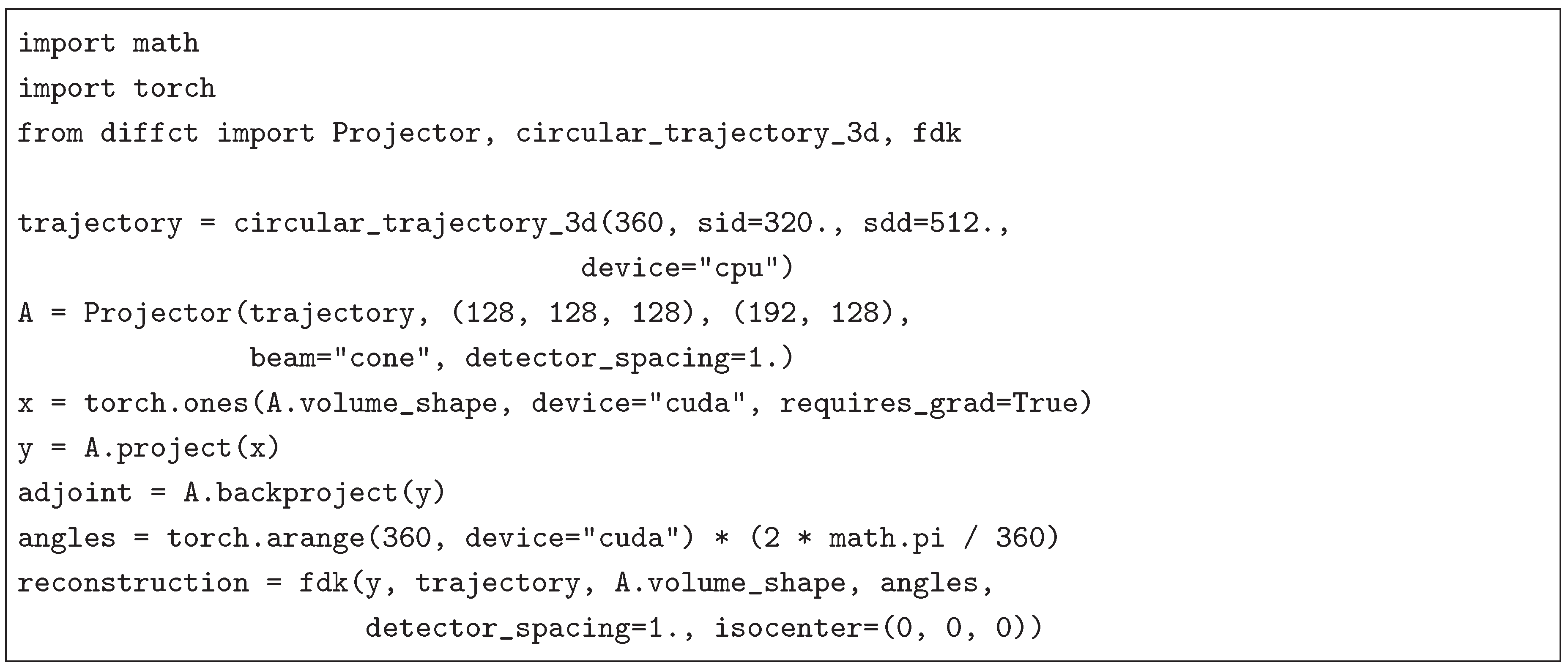
For single-process multi-GPU execution, supply devices=[0,1,...]. For distributed execution, initialize a caller-owned process group, bind each rank to its CUDA device, and supply distributed=True with partition="views" or partition="space". An optional process_group selects the collective group. NCCL uses CUDA collective buffers; Gloo uses CPU staging. Use the ownership and loss rules in Section 7 and Section 7.3. The six exported low-level projector/backprojector Function wrappers implement the same native maps; the configured Projector supplies planning and ownership metadata.

Run the reconstruction examples from a 2.2.1 source checkout, with the installed diffct package or source import resolving to the matching 2.2.1 implementation:

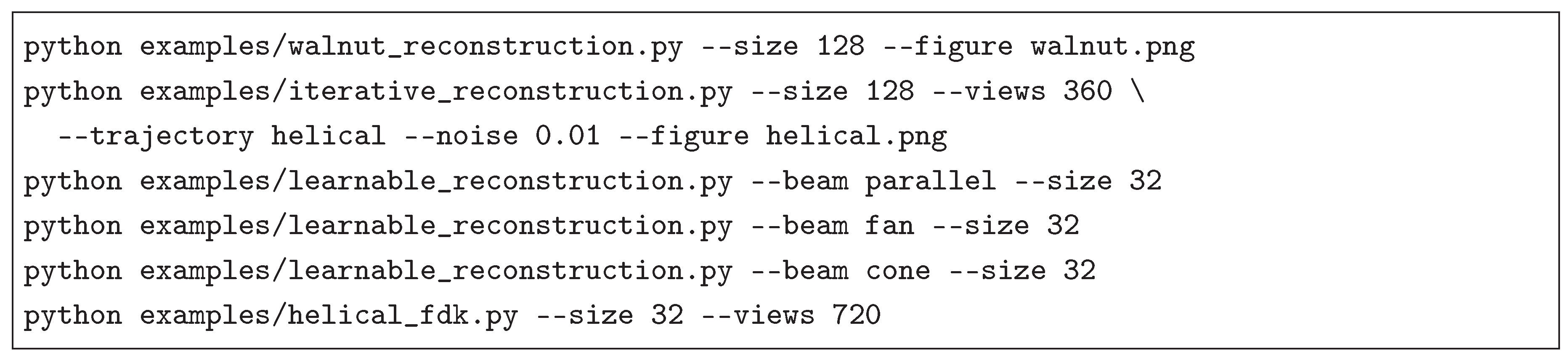
The 2.2.0 scaling script is examples/benchmark_scaling.py; its workload, repeats and CGLS accounting are recorded in Section 8.5. The source package includes the numerical timing samples, calibration samples, regression metrics and saved reconstruction panels used here, identified by source references and hashes. The local report checkout regenerates figures with figures/make_results.py, which reads figures/results/. In the preprint ancillary package, the corresponding copies are anc/make_results.py and anc/results/. Building the report uses latexmk -pdf template.tex. Dataset-derived panels retain the original CC BY 4.0 attribution [24].

References

- Sun, Y. diffct: Differentiable Computed Tomography Reconstruction with CUDA. Zenodo Softw. Release 2025. [Google Scholar] [CrossRef]
- Kak, A.C.; Slaney, M. Principles of Computerized Tomographic Imaging; Society for Industrial and Applied Mathematics: Philadelphia, PA, 2001. [Google Scholar] [CrossRef]
- Paszke, A.; Gross, S.; Massa, F.; Lerer, A.; Bradbury, J.; Chanan, G.; Killeen, T.; Lin, Z.; Gimelshein, N.; Antiga, L.; et al. PyTorch: An Imperative Style, High-Performance Deep Learning Library. Adv. Neural Inf. Process. Syst. 2019, 32, 8024–8035. [Google Scholar]
- Parker, D.L. Optimal Short Scan Convolution Reconstruction for Fanbeam CT. Med. Phys. 1982, 9, 254–257. [Google Scholar] [CrossRef]
- Feldkamp, L.A.; Davis, L.C.; Kress, J.W. Practical Cone-Beam Algorithm. J. Opt. Soc. Am. A 1984, 1, 612–619. [Google Scholar] [CrossRef]
- Tuy, H.K. An Inversion Formula for Cone-Beam Reconstruction. SIAM J. Appl. Math. 1983, 43, 546–552. [Google Scholar] [CrossRef]
- Smith, B.D. Image Reconstruction from Cone-Beam Projections: Necessary and Sufficient Conditions and Reconstruction Methods. IEEE Trans. Med. Imaging 1985, 4, 14–25. [Google Scholar] [CrossRef]
- Siddon, R.L. Fast Calculation of the Exact Radiological Path for a Three-Dimensional CT Array. Med. Phys. 1985, 12, 252–255. [Google Scholar] [CrossRef]
- Long, Y.; Fessler, J.A.; Balter, J.M. 3D Forward and Back-Projection for X-Ray CT Using Separable Footprints. IEEE Trans. Med. Imaging 2010, 29, 1839–1850. [Google Scholar] [CrossRef]
- van Aarle, W.; Palenstijn, W.J.; Cant, J.; Janssens, E.; Bleichrodt, F.; Dabravolski, A.; De Beenhouwer, J.; Batenburg, K.J.; Sijbers, J. Fast and Flexible X-Ray Tomography Using the ASTRA Toolbox. Opt. Express 2016, 24, 25129–25147. [Google Scholar] [CrossRef]
- Biguri, A.; Dosanjh, M.; Hancock, S.; Soleimani, M. TIGRE: A MATLAB-GPU Toolbox for CBCT Image Reconstruction. Biomed. Phys. Eng. Express 2016, 2, 055010. [Google Scholar] [CrossRef]
- Biguri, A.; Lindroos, R.; Bryll, R.; Towsyfyan, H.; Deyhle, H.; Boardman, R.; Mavrogordato, M.; Dosanjh, M.; Hancock, S.; Blumensath, T. Arbitrarily Large Iterative Tomographic Reconstruction on Multiple GPUs Using the TIGRE Toolbox, 2019. arXiv arXiv:cs.
- Syben, C.; Michen, M.; Stimpel, B.; Seitz, S.; Ploner, S.; Maier, A.K. Technical Note: PYRO-NN: Python Reconstruction Operators in Neural Networks. Med. Phys. 2019, 46, 5110–5115. [Google Scholar] [CrossRef]
- Kim, H.; Champley, K. Differentiable Forward Projector for X-ray Computed Tomography. arXiv 2023, arXiv:eess. [Google Scholar]
- Champley, K.; Kim, H. LivermorE AI Projector for Computed Tomography Tasks (LEAP). Software release. 2023. [Google Scholar] [CrossRef]
- Thies, M.; Wagner, F.; Maul, N.; Folle, L.; Meier, M.; Rohleder, M.; Schneider, L.S.; Pfaff, L.; Gu, M.; Utz, J.; et al. Gradient-Based Geometry Learning for Fan-Beam CT Reconstruction. Phys. Med. Biol. 2023, 68, 205004. [Google Scholar] [CrossRef]
- Ye, C.; Schneider, L.S.; Sun, Y.; Thies, M.; Mei, S.; Maier, A.K. DRACO: Differentiable Reconstruction for Arbitrary CBCT Orbits. Phys. Med. Biol. 2025, 70, 075005. [Google Scholar] [CrossRef]
- Paige, C.C.; Saunders, M.A. LSQR: An Algorithm for Sparse Linear Equations and Sparse Least Squares. ACM Trans. Math. Softw. 1982, 8, 43–71. [Google Scholar] [CrossRef]
- Gregor, J.; Benson, T. Computational Analysis and Improvement of SIRT. IEEE Trans. Med. Imaging 2008, 27, 918–924. [Google Scholar] [CrossRef]
- Sidky, E.Y.; Pan, X. Image Reconstruction in Circular Cone-Beam Computed Tomography by Constrained, Total-Variation Minimization. Phys. Med. Biol. 2008, 53, 4777–4807. [Google Scholar] [CrossRef]
- Baydin, A.G.; Pearlmutter, B.A.; Radul, A.A.; Siskind, J.M. Automatic Differentiation in Machine Learning: A Survey. J. Mach. Learn. Res. 2018, 18, 1–43. [Google Scholar]
- Lam, S.K.; Pitrou, A.; Seibert, S. Numba: A LLVM-Based Python JIT Compiler. In Proceedings of the Proceedings of the Second Workshop on the LLVM Compiler Infrastructure in HPC, 2015; pp. 1–6. [Google Scholar] [CrossRef]
- Shepp, L.A.; Logan, B.F. The Fourier Reconstruction of a Head Section. IEEE Trans. Nucl. Sci. 1974, 21, 21–43. [Google Scholar] [CrossRef]
- Meaney, A. Cone-Beam Computed Tomography Dataset of a Walnut, 2022. Version 1.1.0. CC BY 4.0. [CrossRef]
- Kingma, D.P.; Ba, J. Adam: A Method for Stochastic Optimization. In Proceedings of the International Conference on Learning Representations, 2015. [Google Scholar]