

Submitted:
15 May 2026
Posted:
19 May 2026
You are already at the latest version
Abstract
Dirty paper coding (DPC) is applied to linear multi-input multi-output (MIMO) broadcast channels with additive white Gaussian noise and one message per receiver. The method decomposes each receiver channel into parallel scalar channels with known interference, then applies modulo operators, amplitude-shift keying (ASK), and probabilistic shaping. The achievable rate tuples include all points inside the capacity region by choosing truncated Gaussian shaping, large ASK alphabets, and large modulo intervals. Simulations with short polar codes show significant rate gains from DPC compared to conventional linear precoding, while maintaining similar encoder and decoder complexities.
Keywords:
broadcast channel
; capacity
; dirty paper coding
; multi-input multi-output
1. Introduction
This paper is dedicated to Professor H. Vincent Poor on the occasion of his 75th birthday. The authors would like to express their appreciation for his outstanding contributions to engineering research and his unwavering commitment to the information theory and communications communities.
The paper studies the downlink of wireless systems, focusing on how to achieve higher data rates than those achievable with linear precoding (LP) without increasing complexity. Professor Poor authored numerous influential papers on LP and nonlinear processing, covering topics such as multiuser detection [1,2,3], code-division multiple access (CDMA) [4,5,6], orthogonal and non-orthogonal multiple access (OMA and NOMA) [7,8,9,10,10], rate-splitting multiple access (RSMA) [11,12,13], and dirty paper coding (DPC) [14].
1.1. Linear Precoding
LP is a linear version of superposition coding that combines two independently encoded signals. It involves modulating "beams" or vectors and has two basic variants. The first variant, which we focus on, selects one beam per message and maximizes a weighted sum rate while treating interference as noise. This approach is referred to as space division multiple access (SDMA) in [11], but we will refer to it simply as LP. The second variant avoids interference by using orthogonal beams, such as time- or frequency-division multiplexing, and is often called OMA. It is worth noting that SDMA, OMA, and other variants of LP can achieve higher rates by utilizing multiple transmission modes with optimized resource allocation across time, frequency, and power [15]. Different transmission modes can be represented by an auxiliary random variable [16] [p. 278], which is generally preferable to using a convex hull operator; see [16] [p. 288]. However, adding modes introduces latency.
SDMA and OMA are commonly used in practice, but they yield suboptimal results. An LP variation that achieves the capacity of broadcast channels (BCs) with single-antenna transceivers utilizes successive interference cancellation (SIC), as discussed by Cover [17] [Sec . VII], Bergmans [18,19], Gallager [20], and others [21,22]. In this approach, each UE first decodes a set of signals intended for other UEs, then cancels the interference from those signals before decoding its own signal. This method is commonly referred to as NOMA. However, SIC increases the complexity and latency for the UEs.
A variation of NOMA involves splitting each message into multiple parts, encoding them separately, and decoding them individually. This approach effectively increases the total number of messages being transmitted. Message splitting was introduced by Carleial for interference channels [23] and was applied to broadcast channels around the same time; see [24] [Sec. III]. This general method is sometimes referred to as RSMA [11,12,25]. RSMA increases both the complexity and latency of base stations (BSs) and user equipments (UEs), but it can offer performance advantages over DPC when channel state information at the transmitter (CSIT) is imperfect [26,27].
The most general approach combines superposition coding with DPC, and we refer to this method as Marton coding [28]; see also [16] [p. 391]. Marton coding can be implemented by targeting specific corner points of the rate region using DPC, and then applying time-sharing. We remark that time-sharing latency can be significantly reduced by utilizing fine time-shifts and alternating DPC [29].
1.2. Dirty Paper Coding
DPC arises in the context of channels with non-causal state information at the transmitter, for which the capacity was characterized by Gelfand and Pinsker [30]. Costa applied the theory to additive white Gaussian noise (AWGN) channels with additive Gaussian interference known at the transmitter. Remarkably, the capacity is the same as without interference [31], a result similar to Wyner-Ziv coding for Gaussian sources and mean square error distortion [32]. The result was later extended to general interference by using high-dimensional lattices [33,34].
DPC achieves all points in the capacity region of a linear, multi-input multi-output (MIMO), AWGN BC with independent messages, each destined for a different receiver [35,36,37,38,39,40,41]. The idea is to encode the messages successively, treating the signals of previously encoded messages as interference. One thereby achieves higher rates than LP. However, DPC is rarely used in practice because it is considered too complex. We argue here that DPC can be implemented with a similar level of complexity to coded LP, albeit with higher latency due to successive encoding.
A useful insight for understanding DPC is that successive encoding is the dual of successive decoding at the receiver of an appropriate (dual) multiple-access channel (MAC) [39]. Remarkably, Gaussian signaling, linear minimum mean-square error (LMMSE) estimation, and convex optimization yield the best MAC rates, and the best MAC beamforming vectors can be transformed into the best BC precoding vectors. A refined approach decomposes the BC into scalar channels and shows that the best BC precoding and MAC beamforming vectors are co-linear [42].
1.3. Code Constructions
Explicit DPC constructions are described in [43,44,45,46]. These papers use low-density parity-check (LDPC) or turbo codes for reliability and trellis codes for shaping. The schemes require long block lengths, and the complexity is high. Similarly, the superposition coding scheme in [47] employs long LDPC and trellis codes. Lattice constructions with integer-forcing were proposed in [48,49,50,51]; these perform well, but typically do not achieve capacity. Non-asymptotic analyses of random coding are described in [52,53,54,55,56,57,58,59,60].
Polar codes [61] are an attractive alternative because they permit practical nested coding for reliability, quantization, and shaping. The paper [62] analyzes binary DPC, the paper [63] shows how to perform shaping, the paper [64] introduces polar coded modulation, and the thesis [65] designs polar lattices for DPC; see also [29,66,67,68,69,70,71,72,73,74,75,76] and [77,78,79,80,81,82]. We also use polar codes, but with scalar modulo operations, dithering, and probabilistic shaping [57,59]. A modulo operator reduces the transmitter dynamic range, and dithering decouples the constellation and interference statistics, which provides useful independencies.
1.4. Organization and Contributions
This paper is organized as follows. Section 2 reviews notation and results on symmetric unimodal functions. Section 3 describes the vector BC and shows that noise whitening and the singular value decomposition (SVD) give parallel scalar channels with known interference. One may thus apply scalar DPC to achieve all rate tuples in the capacity region [83]. Section 4 and Section 5 prove that the scalar coding scheme in [59] achieves these rate tuples. Section 7 designs short polar codes and provides frame error rate (FER) curves based on numerical simulations. Section 8 concludes the paper.
2. Preliminaries
2.1. Notation
Column vectors are denoted as , where is the transpose of . Bold letters such as denote matrices; is the complex-conjugate transpose of ; is the trace of ; is the determinant of ; is an identity matrix. We write , , and
where is the integer so that lies in .
Upper- and lowercase letters denote random variables (RVs) and their realizations; e.g., is a random vector and is its realization. denotes the probability density function of the random variable X. We remove subscripts if the argument is a lowercase version of the RV, e.g., . Define the expectation and entropy with respect to a density as
We write and if the density is clear from the context. denotes the mutual information of X and Y. denotes the Q-function.
2.2. Decomposition of a Covariance Matrix
Let and be the mean and covariance matrix of . The matrix is positive semi-definite and has the eigenvalue decomposition
where is unitary and is diagonal with non-negative entries. Suppose there are positive eigenvalues. Let be the matrix with these eigenvalues, and let be the matrix with the corresponding columns of removed. Then a Cholesky decomposition is
for any unitary matrix . Observe that is an matrix with the left inverse
For example, if and then . In this case, one usually writes and .
2.3. Symmetric and Unimodal Functions
The real-valued function is symmetric if for all . The following (known) lemma is proved in Appendix A.
Lemma 1.
The convolution of two symmetric functions and is symmetric.
We study symmetric and unimodal probability density functions (p.d.f.s) , i.e., is non-increasing for . The following lemma was proved in [84, pp. 30-32] and [85, Thm. 2.1]; Appendix A provides an alternative proof.
Lemma 2.
The convolution of two symmetric unimodal p.d.f.s and is symmetric unimodal.
Finally, we derive bounds on the sum of uniformly spaced samples of a symmetric unimodal function . Appendix A proves the following lemma for the spacing .
Lemma 3.
Consider a symmetric unimodal . We have
for x satisfying . Similarly, if has finite area then for any x we have
2.4. Scalar DPC Scheme
We review the scalar DPC scheme from [59]. Consider the real-alphabet additive noise channel
where X satisfies the power constraint , S is interference known at the transmitter, and Z (not necessarily Gaussian) is independent of and has variance . The encoder computes [59] [eq. (1)]
where the dither D is continuously uniform over the interval . Consider a shaping density . A symbol U is selected from the M-ASK constellation
by using the discrete shaping distribution
Note that is the ASK-spacing. The transmitted signal is (see [59, eq. (2)])
where . The shaping (12) induces the input distribution
where
The received signal is (see [59] [eq. (3)-(4)])
where the effective noise is
with variance .
3. Gaussian Vector Broadcast Channels
Consider a complex-alphabet BC with the -dimensional input and -dimensional outputs
where is an complex matrix and is a circularly-symmetric, complex, Gaussian (CSCG) noise vector with invertible covariance matrix . We require to satisfy the power constraint .
Consider one message per UE with rate for all k. Let be an covariance matrix associated with message k. The following rate tuples are achievable by considering the UE ordering and treating the messages l with as being known at UE k:
subject to . The capacity region is the union of all such rate tuples, taken over all and UE orderings; see [28,40].
3.1. Capacity-Achieving Scheme
The BS sends where the are statistically independent [39] and each has an covariance matrix optimized for a particular rate tuple. The optimal are CSCG. Using (5), we have
where , , and have dimensions , , and , respectively. It suffices to consider for all k.
Consider the ordering . UE k sees
and treats as interference and as noise. Let be the covariance matrix of . We use the SVD to write
where and are unitary and is an diagonal matrix with the singular values of . Now choose in (23). UE k left-multiplies with the dimensional noise-whitening filter
to obtain the parallel channel
where is known at the BS and
Note that only the first entries of are useful channel outputs, i.e., we have useful sub-channels.
The covariance matrices of and are identity matrices, i.e., the entries , , and , , are independent and identically distributed (i.i.d.) CSCG with unit variance. The power constraint is where . The BS can use as an precoding matrix to compute .
3.2. Parallel DPC with Scalar Modulo Operations
The are independent since the are independent. Moreover, the decomposition (27) specifies sub-channels where the ith entry of is
for and . The parameter is a singular value, is known at the BS, and is CSCG and independent of . Thus, one achieves capacity if one achieves the capacity for each scalar channel (29) in (27), and for the covariance matrices of all required rate tuples.
One may write where the entries of are i.i.d. CSCG with unit variance. Thus, using (24) and (28), we have
Alternatively, there are constants and for which
We apply the DPC in [57] to each channel (29) by treating the real and imaginary parts of as independent with the same channel gain and noise variance . We focus on the real part and abuse notation by using the same symbols as for the complex alphabet channels, i.e., all random variables are now real-valued. Also, the , , and are no longer Gaussian, with the exception of the .
More precisely, consider the real part of sub-channel and define
where
Now code as in Section 2.4, where we identify and the parameters
Note that Z is not necessarily Gaussian. We choose the across the sub-channels as independent, which makes the independent for all ; see Appendix B. Thus, all RVs on the right-hand side of (31) are independent and the density of is the convolution of the densities of the and (more generally, if a does not have a density, the density of is the derivative of the convolution of the distribution functions of the and ).
Lemma 4
(cf. [59, Lemma 2]). Consider fixed . In the limit of large , we have for all x.
Theorem 1
(cf. [59, Theorem 1]). Consider the DPC scheme in Section 2.4 applied to all sub-channels. For each sub-channel, consider the variables (33)–(34) and the shaping density (18). Given A, the parameter is chosen so that (19) takes on the value . Let
be an -tuple of achievable rates for the specified parameters
Given , there is a sequence of achievable rates satisfying
for all . Moreover, for each sub-channel, we have and as , yielding
Note that (35) specifies achievable rates for finite . This bound can thus be used for peak power constraints.
4. Proof of Lemma 4
Consider in (15), and recall that for a unique integer . We have
where step follows because the modulo operator permits summing over any M successive integers. Thus, is periodic with period . For example, Figure 1 shows for , , and the truncated Gaussian in [59] [eq. (11)] with . Note that satisfies (37) for general and not just a truncated Gaussian .
Suppose is symmetric, which means that and are symmetric. For , we have
Now suppose is symmetric and unimodal. Applying (7) in Lemma 3, we have for all x, where
We thus have for and
where we assume M is sufficiently large so . Figure 2 illustrates the bounds (40) for , , and the truncated Gaussian in [59, Equation (12)] with . We compute and . The bounds are loose because M is relatively small.
We derive more properties of for the truncated Gaussian . The derivative of (38) for is
and, by symmetry, we have . Consider first odd M and ; the positive and negative summands cancel and ; see Figure 1. For even M, there is a summand at but not at . Thus, for small positive x. By symmetry, we thus have for small negative x; see Figure 1.
5. Proof of Theorem 1
We use the definitions (33)-(34). Observe that we have
The achievable rate of sub-channel is [eq. (5) [59]
We anticipate the result as follows. Section 5.2 shows that , which cancels for large M. Section 5.1 shows that if M is large and and . Section 5.3 shows that the latter two approximations are valid for large A. Finally, we have the upper bound
Step follows because a zero-mean Gaussian maximizes entropy under a second-moment constraint, and step follows from ; see (17) and (42).
The following two sections first study and and then and .
5.1. Power and Differential Entropy of X
The power is based on an expectation with respect to . Using (2) and (40), for symmetric unimodal , we have
and thus for . Using (40), we have (see Appendix C)
and for , we have (see ())
5.2. Density and Differential Entropy of
Consider in (16) where U and in (17) are independent. Note that Z is the sum of one Gaussian and several shaped random variables; see (31) and (33).
Suppose M is even; the case where M is odd can be treated similarly. Using symmetric shaping for each sub-channel and Lemma 1, it follows that and
for and otherwise. Hence, is symmetric and periodic with period in . Figure 3 illustrates these results for a point-to-point channel with , , , , Gaussian, and . We show next that in if M is large. In fact, increasing M to 8 in Figure 3 already gives .
The density is the convolution of three classes of densities, namely those of:
- ,
- the for and all h, and
- the for all h.
The densities and are chosen to be symmetric unimodal, but the densities of and are not necessarily unimodal. However, the latter densities can each be lower-bounded by appropriate and as in (40), and these bounds are symmetric unimodal. Moreover, the Gaussian densities of the are symmetric unimodal. Thus, by Lemma 2 and using (39)–(40), we can lower bound by a symmetric unimodal that approaches for large M. Similarly, we can upper bound by a symmetric unimodal that approaches for large M. That is, we obtain
for symmetric unimodal and that both converge to for large M.
For example, point-to-point DPC has the effective noise where X and Z are independent; see (17). We hence have the convolution
Note that is symmetric but not necessarily unimodal, and hence is symmetric but not necessarily unimodal. However, we may bound
where step follows by (40) and step uses the density
which is symmetric unimodal in x. The function defined in (51) is a convolution of two symmetric unimodal functions. Thus, is symmetric unimodal by Lemma 2. Moreover, one can iterate the above argument for successive DPC with , and thereby obtain a symmetric unimodal with .
Let be the same as but with replacing in (51). We have the bounds (49) where both and are symmetric unimodal. Figure 4 shows the curves for , , the truncated Gaussian with , , , and Z is Gaussian.
Now substitute and for in (8) of Lemma 3 to write
for any . Define the expressions
Applying (53) gives
for , where steps and follow by (48a) and (49). For example, for the parameters in Figure 3, we have and . The bounds are again loose because M is small. However, as , we have , and hence converges to the uniform distribution over . Finally, assuming M is sufficiently large such that , we obtain
which implies for .
5.3. Achieving Capacity
For fixed A, satisfying , and , we obtain the bound (35) by using (44), (47), and (56). Finally, consider three possible scalings as :
6. Simulation Models and Capacity
Consider a BS serving UEs, each with antenna. We have and
where each is a column vector of dimension , and .
6.1. DPC and Duality
The DPC rate bounds (22) simplify to
The optimal precoders can be found by using the dual MAC with output
and independent inputs , with variances , that satisfy ; see [39]. The noise has i.i.d. entries with unit variance. Let and be MAC receiver beamforming vectors that create the scalar outputs
for UEs 1 and 2, respectively. The optimal are specified by LMMSE estimation; see Appendix D. It remains to determine the powers and , which turns out to be a concave optimization problem in general.
Next, following [42], we choose the BC precoding vectors as co-linear with the :
for real scalars . Suppose the BC first encodes for UE 1, and the MAC receiver first decodes the UE 2 signal. For the desired rate equivalences, we require the signal-to-interference-and-noise ratios (SINRs) to satisfy
where the left- and right-hand sides are BC and MAC SINRs, respectively. Using , we obtain
and thus
For example, consider the channel vectors
with , , and . We use the dual MAC to compute the capacity region shown in Figure 5. This region is the union of two regions corresponding to the two encoding orders, which are shown as dashed lines.
6.2. Coded LP
We compare with linear precoding (LP) where the transmit vector is with independent . The bound (22) becomes more restrictive:
where the denominator sum is now over . For example, for and , the bounds are (see (62))
Appendix E reviews a BC-MAC duality for coded LP. The optimal beamforming vectors in (64) for the dual MAC are again specified by LMMSE estimation, and we may again use the relations (65); see [42]. Unfortunately, unlike DPC, the power allocation problem is no longer concave. We thus perform an exhaustive search over a fine quantization of power allocations, which is possible for small numbers of UEs and antennas. The LP region for the channels (69) with , , and is shown in Figure 5.
We remark that coded LP can be improved, see Section 1.1. For example, one may use multiple transmission modes, as well as RSMA and SIC; see Appendix F-Appendix G. However, SIC increases UE complexity and latency.
6.3. Computing Rate Regions
We study parallel channels for the polar code simulations, e.g., corresponding to tones in an orthogonal frequency-division multiplexing (OFDM) system. A BC with two transmit antennas, one antenna per UE, and two tones may be written as having and , where the rows of each are orthogonal.
For example, consider
For DPC, we use the dual MAC and optimize weighted sum rates over
- the power allocation across the parallel MACs;
- the users’ transmit powers for the two MACs;
- the MAC decoding orders.
One can apply any convex solver, e.g., gradient descent [86]. For coded LP, one may consider either the BC or dual MAC and optimize the weighted sum rate over
- the power allocation across the parallel MACs;
- the users’ transmit powers for the two MACs.
We use the dual MAC and LMMSE estimation, see Section 6.2, and perform an exhaustive search over a fine quantization of power allocations. For problems with more UEs and antennas, one must resort to other methods, e.g., gradient-based methods as in [87].
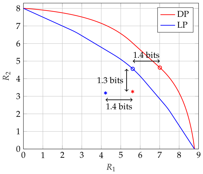
The capacity and LP rate regions are plotted in Figure 6. The circles show points that maximize the sum rates for DPC and coded LP, namely
The asterisks show points targeted for the polar code simulations in Section 7, namely
Figure 6.
Capacity and LP rate regions for the channels (72). Circles show points that maximize the sum rate and are targeted for the polar code simulations. Asterisks show the rates achieved by polar codes of length 256 bits when the target FER for each user is .
Figure 6.
Capacity and LP rate regions for the channels (72). Circles show points that maximize the sum rate and are targeted for the polar code simulations. Asterisks show the rates achieved by polar codes of length 256 bits when the target FER for each user is .
6.4. Polar Code Simulations
We use the channel (Section 6.3) with to perform polar code simulations described in Section 7. We target the maximum sum rate via the DPC order 1,2, and apply the steps in Section 3.1. The resulting singular values for the sub-channels (29) are
For coded LP, the optimized precoders are used to compute the covariance matrices , and then the steps in Section 3.1 are used to compute the singular values with no interference and enhanced noise
The resulting singular values for the best sum rate are
7. Short Polar Codes
Let for a positive integer n. The polar encoding matrix is
where denotes an n-fold Kronecker product. An N-dimensional bit vector is encoded as . The recursive block structure of yields
and thus and are the codewords obtained by encoding the first and second halves of , respectively. Thus, is constructed by first encoding the subblocks and , and then applying a polarization transform to combine these subcodes. For example, Figure 7 shows that the encoder can first map and to and , respectively, and then apply one level of the polarization transform () to the corresponding sub-codeword elements. We exploit this structure to construct a long polar code across two sub-channels of a UE by using two separate polar sub-codes.
7.1. Shaped Multi-Level Coding
There are two variants of shaping with polar codes: all coded bits are assigned the same or different a priori distributions. The former approach applies to time-invariant coding, and the latter to time-varying coding. An example of a time-varying coding is DPC, because the interference varies with each coded bit.
We use shaped multi-level coding (MLC) to map message bits to ASK symbols. A simple approach uses separate polar codes for each sub-channel. However, at short block lengths, performance improves by using a single, long multi-level polar code across all sub-channels of a user.
Another effective approach leverages the different singular values in (29), to enhance polarization [60,72,88]. Let , , denote the mutual information of the polar code bit channels, ordered such that for . Further, let and denote the indices of the least reliable and most reliable code bit channels, respectively, with in ascending order and in descending order. By matching the corresponding elements of and in the last polarization stage, the FER performance of the polar code can be improved. For example, in Figure 7, the code bits transmitted on are matched in the last polarization stage with the code bits transmitted on , respectively.
7.2. Polar Coded Modulation
The BS sends 64 symbols , . Alternatively, for our example channel (72), it sends 64 symbols over each of the parallel channels with inputs
We choose the and in DPC to have a 256-QAM alphabet, while all other have a 64-QAM alphabet. These alphabets are split into two real alphabets: 16-ASK and 8-ASK. There are, therefore, 128 real symbols for fixed and . We map these 128 symbols to the complex QAM symbols via
for . The precoded transmit vectors are
for and . The BS in DPC thus sends and coded bits over the sub-channels of UE 1 and UE 2, respectively, corresponding to a total of 1024 and 768 coded bits for UE 1 and UE 2, respectively. The BS uses MLC with 4 or 3 levels across sub-channel pairs, and each level has 256 coded bits.
Consider DPC with the precoding order . The message bits of UE 1 are encoded directly into the 256 real 16-ASK symbols in the order
by using MLC with 4 levels and a length-256 polar code for each level. From (80) and (81), the first and second halves of the polar code bits protecting the bit levels of are transmitted over sub-channels with channel coefficients and , respectively; see (27).
Let be the 128-dimensional vector with 128 ones. The encoding parameters for the two sub-channels of UE 2 can be interpreted as the 256-dimensional vectors
For UE 2, the BS treats as interference; see (30). To encode to 256 real 8-ASK symbols , the BS applies
for and . To simplify notation, write the 256 coded bit indexes as and define
Note that we used the same ordering as above for . Similarly write
The BS performs shaping by computing the log-likelihood ratio (LLR)
of the coded bit at the lth bit-level, , , where we used the shaping density (18) and similar notation as (82)-(85). A polar decoder treats both the frozen and message bits as frozen to compute the shaping bits. The set in (89) is the subset of 8-ASK symbols for which the first l labeling bits are .
7.3. Simulation Results
The modulo operator limits the dynamic range at the UEs and BS, especially in the presence of interference. However, the dispersion increases at low rates, and this increases the FER at short block length [59, Figure 5 and Figure 6]. We therefore use a modulo operator for DPC only, i.e., we do not use a modulo interval for UE 1 under DPC, or for either UE in the LP scheme. Instead, we shaped with a sampled Gaussian distribution proportional to with . The ASK spacings were and for and 16, respectively. For UE 2 with DPC, we cancel interference by shaping according to (12), and use and for both sub-channels.
We allocate an asymptotically optimal fraction of sub-channels to shaping at each bit level; see [57, Sec. IV]. For the two polar subcodes corresponding to bit level , the mutual information is computed from this quantity and translated proportionally into the fraction of shaping bits assigned to each subcode. Within each bit level, the most reliable sub-channels are allocated to the shaping bits, the next most reliable sub-channels to the message bits, and the remaining sub-channels to the frozen bits. The sub-channel reliability order specified in 5G NR [89] is used. We employ 6 CRC bits, which are transmitted on the reliable subcode of the last bit level. At this level, after allocating the shaping bits, the most reliable remaining sub-channels are assigned to the CRC bits. Natural labeling maps bits to modulation symbols.
After allocating the shaping and CRC bits, the assignment of message bits to the bit levels and their subcodes is optimized to maximize the achievable information rate (AIR) at a target FER of for a total transmit power . The resulting parameters are given in Table 1, where and are the numbers of shaping and information bits at bit level i, respectively, and “sub” indicates the subcode index. The parameters in Table 1 would make the variances of the slightly larger than one due to finite block length shaping, so we normalize so that the have unit variance.
The BS uses successive cancellation (SC) decoding for shaping, and the UEs use SC list decoding with list passing [57] across subcodes and bit levels for channel decoding.
Figure 8 plots the FER versus . The UE codes are designed at , or dB, and achieve the target error rate . The precoders are optimized for each SNR value. Overall, DPC transmits a sum of 568 bits to both UEs over 64 channel uses, with a sum rate of bits per channel use (bpcu); see Figure 6. Coded LP transmits 474 bits, yielding a total rate of bpcu, so DPC gains bpcu. The asymptotic rates at for DPC and coded LP are approximately bpcu and bpcu, respectively, so DPC gains bpcu.
8. Conclusions
We showed that scalar DPC based on modulo operations, probabilistic shaping, and dithering can approach any rate tuple in the capacity region of a complex-alphabet MIMO BC with CSCG noise and one message per receiver. The encoder and decoder complexities are similar to those of coded LP. Short polar code simulations demonstrate the rate gains achieved through DPC relative to coded LP. Future work may derive better bounds on the achievable rates, e.g., by using informational divergence rather than bounds based on symmetric unimodal functions.
Author Contributions
Conceptualization, M.Y.Ş. and G.K.; methodology, M.Y.Ş., G.K., and R.B.; software, M.Y.Ş.; validation, M.Y.Ş., G.K., S.S., R.B., and W.X.; formal analysis, M.Y.Ş. and G.K.; investigation, M.Y.Ş.; resources, R.B. and W.X.; data curation, M.Y.Ş.; writing—original draft preparation, M.Y.Ş. and G.K.; writing—review and editing, M.Y.Ş., G.K., S.S., R.B., and W.X.; visualization, M.Y.Ş. and G.K.; supervision, G.K., R.B., and W.X.; project administration, M.Y.Ş. and G.K.; funding acquisition, G.K., S.S. All authors have read and agreed to the published version of the manuscript.
Funding
This work was supported by the German Research Foundation (DFG) via the German-Israeli Project Cooperation (DIP) under Projects KR 3517/13-1 and SH 1937/1-1.
Conflicts of Interest
The authors declare no conflict of interest.
Appendix A. Proof of Lemmas
Appendix A.1. Proof of Lemma 1
If and are both symmetric then
where step follows by symmetry and step follows by substituting .
Appendix A.2. Proof of Lemma 2
Unimodality implies that can have a Dirac-delta component at only, i.e., one may write
for a constant satisfying , and for a non-negative, symmetric, unimodal without components. We may assume the derivative exists almost everywhere [Prop. 2.1 [85]. The x where does not exist include “jumps" in . For example, a negative “jump" at from to , where is a vanishing positive number and , becomes a component in .
As in (A2), consider . We compute
which is symmetric; see Lemma 1. The first three summands in (A3) are unimodal, so it remains to show that is unimodal. Taking the derivative for , we have
where step follows by substituting and because and are symmetric. But the term in square brackets is non-negative because and is symmetric unimodal. We also have for because is symmetric unimodal.
Appendix A.3. Proof of Lemma 3
The sum in (7) is a Riemann sum, so we use the left and right rules of Riemann summation. Figure A1 shows a symmetric unimodal for (here is a truncated Gaussian density). The sample points for are located at the top-left corner of each of the six bars. The area of each bar is one of the summands in (7); the area of the green bar is at most . Figure A1 shifts the red bars of positive sampling points to the left by , and we see that the area of the five red bars is less than the integral in (7). This can be done for any x with , so the sum in (7) is at most the integral plus .
Figure A1.
for . The sampling points are shifted by x = 0.2, and are located at the top left corner of each of the six bars.
Figure A1.
for . The sampling points are shifted by x = 0.2, and are located at the top left corner of each of the six bars.
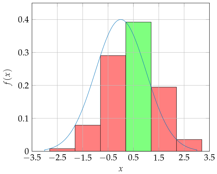
Figure A2.
for . The area of the red bars is less than the area of , which is here 1.
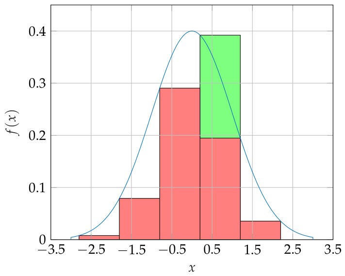
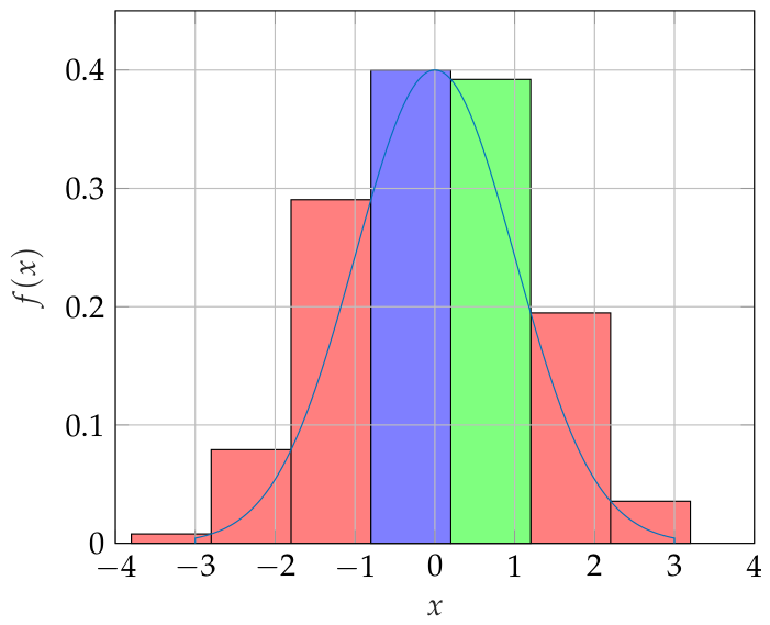
Similarly, Figure A3 shifts the red bars of negative sampling points to the left by so they lie above . If we add one (blue) bar of area , then the sum of the areas of the seven bars is greater than the integral in (7). This proves (7). To prove (8), we perform similar steps with a countable number of bars and appropriate left and right shifts. Note that we may restrict attention by symmetry.
Figure A3.
for . The area of the red, green, and blue bars is greater than the area of , which is here 1.
Figure A3.
for . The area of the red, green, and blue bars is greater than the area of , which is here 1.
Appendix B. Independence of the Channel Inputs X ˜ k,i
Let be the vector of all except . Note from (24) that is a function of . Moreover, the chain is Markov because is chosen using as shown in (12). Suppose the dithers are mutually independent, and consider the identities
where step follows because is a discrete RV given (see (13)), step follows by (12), (14), and (15) and step follows because and (see (14)). Thus, the channel inputs in (29) are mutually independent.
Appendix C. Entropy Bounds
Appendix D. MAC Beamformers
The best MAC receiver beamformers are LMMSE filters. Let be the covariance matrix of . The LMMSE operation is the conditional expectation with the LMMSE filters
For example, for the channels (69), if the receiver decodes UE 1’s signal first, we have
Similarly, decoding UE 2’s message first, we have
Observe that is matched to for small , and is orthogonal to for large . Moreover, the LMMSE filter for transmitter 2, after removing the interference of transmitter 1, is matched to . Similarly, is matched to for small , and is orthogonal to for large . The LMMSE filter for transmitter 1, after removing the interference of transmitter 2, is matched to .
Appendix E. Dual MAC for coded LP
Consider the dual MAC, beamforming, and scaling in (63)–(65). The new SINR equivalences are (cf. (66) and [42])
These equations simplify to
Rearranging, we obtain
and directly see the power equivalence (cf. (68))
The matrix in (A12) has an inverse with positive entries. Non-negative thus give non-negative . The reverse may be seen by writing where and inserting into (A11). We obtain
where . Note that swapping with does not change the equations. Thus, non-negative give non-negative ; see (A12).
Appendix F. Information Rates of LP with Two Modes
Consider LP with UEs and two transmission modes that are given fractions and of the time/frequency resources. One may optimize over , and the covariance matrices of each mode . An achievable weighted sum-rate is characterized by the problem:
where
For example, for the channels (69) with , one should optimize and the angles and powers of four precoding vectors (two precoding vectors for each UE).
Appendix G. Rate Splitting
Consider independent vectors with . The BS transmits
The idea is to split each message k into up to different messages, each carried by exactly one of the with . UE k decodes these , either using joint decoding or SIC. Clearly, the number of parameters and bounds grows rapidly with K. For , we have three messages and (70) is replaced with four decoding bounds:
for . We also have three rate-splitting bounds
For example, setting , we have and obtain the two LP bounds (70). A more interesting case is so that and one chooses
In this case, UE 2 recovers both messages. As for coded LP, time- or frequency-sharing across multiple transmission modes can increase coded LP rates; see [15].
References
- Poor, H.; Verdu, S. Single-user detectors for multiuser channels. IEEE Trans. Commun. 1988, 36, 50–60. [CrossRef]
- Poor, H.; Verdu, S. Probability of error in MMSE multiuser detection. IEEE Trans. Inf. Theory 1997, 43, 858–871. [CrossRef]
- Wang, X.; Poor, H. Blind multiuser detection: a subspace approach. IEEE Trans. Inf. Theory 1998, 44, 677–690. [CrossRef]
- Mitra, U.; Poor, H. Adaptive receiver algorithms for near-far resistant CDMA. IEEE Trans. Commun. 1995, 43, 1713–1724. [CrossRef]
- Nelson, L.; Poor, H. Iterative multiuser receivers for CDMA channels: an EM-based approach. IEEE Trans. Commun. 1996, 44, 1700–1710. [CrossRef]
- Wang, X.; Poor, H. Iterative (turbo) soft interference cancellation and decoding for coded CDMA. IEEE Trans. Commun. 1999, 47, 1046–1061. [CrossRef]
- Ding, Z.; Yang, Z.; Fan, P.; Poor, H.V. On the performance of non-orthogonal multiple access in 5G systems with randomly deployed users. IEEE Signal Proc. Lett. 2014, 21, 1501–1505. [CrossRef]
- Ding, Z.; Adachi, F.; Poor, H.V. The application of MIMO to non-orthogonal multiple access. IEEE Trans. Wireless Commun. 2015, 15, 537–552. [CrossRef]
- Ding, Z.; Liu, Y.; Choi, J.; Sun, Q.; Elkashlan, M.; Chih-Lin, I.; Poor, H.V. Application of non-orthogonal multiple access in LTE and 5G networks. IEEE Commun. Mag. 2017, 55, 185–191. [CrossRef]
- Vaezi, M.; Schober, R.; Ding, Z.; Poor, H.V. Non-orthogonal multiple access: common myths and critical questions. IEEE Wireless Commun. 2019, 26, 174–180. [CrossRef]
- Clerckx, B.; Mao, Y.; Schober, R.; Poor, H.V. Rate-splitting unifying SDMA, OMA, NOMA, and multicasting in MISO broadcast channel: a simple two-user rate analysis. IEEE Wireless Commun. Lett. 2020, 9, 349–353. [CrossRef]
- Park, J.; Choi, J.; Lee, N.; Shin, W.; Poor, H.V. Rate-splitting multiple access for downlink MIMO: a generalized power iteration approach. IEEE Trans. Wireless Commun. 2023, 22, 1588–1603. [CrossRef]
- Wang, C.X.; You, X.; Gao, X.; Zhu, X.; Li, Z.; Zhang, C.; Wang, H.; Huang, Y.; Chen, Y.; Haas, H.; et al. On the road to 6G: visions, requirements, key technologies, and testbeds. IEEE Commun. Surveys & Tutor. 2023, 25, 905–974. [CrossRef]
- Katz, A.; Peleg, M.; Vincent Poor, H.; Shamai Shitz, S. The Gaussian primitive discrete time and filtered diamond channel: correlated noise and dirty-paper coding. IEEE Trans. Commun. 2025, 73, 5495–5508. [CrossRef]
- Bergmans, P.; Cover, T. Cooperative broadcasting. IEEE Trans. Inf. Theory 1974, 20, 317–324. [CrossRef]
- I. Csiszár and J. Körner. Information Theory: Coding Theorems for Discrete Memoryless Channels; Akadémiai Kiadó: Budapest, 1981.
- Cover, T. Broadcast channels. IEEE Trans. Inf. Theory 1972, 18, 2–14. [CrossRef]
- Bergmans, P. Random coding theorem for broadcast channels with degraded components. IEEE Trans. Inf. Theory 1973, 19, 197–207. [CrossRef]
- Bergmans, P. A simple converse for broadcast channels with additive white Gaussian noise. IEEE Trans. Inf. Theory 1974, 20, 279–280. [CrossRef]
- Gallager, R.G. Capacity and coding for degraded broadcast channels. Probl. Peredachi Inf. 1974, 10, 3–14.
- Cover, T. An achievable rate region for the broadcast channel. IEEE Trans. Inf. Theory 1975, 21, 399–404. [CrossRef]
- van der Meulen, E. Random coding theorems for the general discrete memoryless broadcast channel. IEEE Trans. Inf. Theory 1975, 21, 180–190. [CrossRef]
- Carleial, A. Interference channels. IEEE Trans. Inf. Theory 1978, 24, 60–70. [CrossRef]
- Gamal, A. The capacity of a class of broadcast channels. IEEE Trans. Inf. Theory 1979, 25, 166–169. [CrossRef]
- Joudeh, H.; Clerckx, B. Sum-rate maximization for linearly precoded downlink multiuser MISO systems With partial CSIT: A rate-splitting approach. IEEE Trans. Commun. 2016, 64, 4847–4861. [CrossRef]
- Mao, Y.; Clerckx, B.; Li, V.O. Rate-splitting multiple access for downlink communication systems: Bridging, generalizing, and outperforming SDMA and NOMA. EURASIP J. Wireless Commun. Netw. 2018, 2018, 133.
- Mao, Y.; Clerckx, B. Beyond dirty paper coding for multi-antenna broadcast channel With partial CSIT: a rate-splitting approach. IEEE Trans. Commun. 2020, 68, 6775–6791. [CrossRef]
- Marton, K. A coding theorem for the discrete memoryless broadcast channel. IEEE Trans. Inf. Theory 1979, 25, 306–311. [CrossRef]
- Runge, C.; Kramer, G. Time-shifted alternating Gelfand-Pinsker coding for broadcast channels. In Proceedings of the IEEE Int. Symp. Inf. Theory, Athens, Greece, 2024; pp. 1700–1705. [CrossRef]
- Gelfand, S. Coding for channel with random parameters. Probl. Contr. Inf. Theory 1980, 9, 19–31.
- Costa, M. Writing on dirty paper. IEEE Trans. Inf. Theory 1983, 29, 439–441. [CrossRef]
- Wyner, A.; Ziv, J. The rate-distortion function for source coding with side information at the decoder. IEEE Trans. Inf. Theory 1976, 22, 1–10. [CrossRef]
- Zamir, R.; Shamai, S.; Erez, U. Nested linear/lattice codes for structured multiterminal binning. IEEE Trans. Inf. Theory 2002, 48, 1250–1276. [CrossRef]
- Erez, U.; Shamai, S.; Zamir, R. Capacity and lattice strategies for canceling known interference. IEEE Trans. Inf. Theory 2005, 51, 3820–3833. [CrossRef]
- Yu, W.; Sutivong, A.; Julian, D.; Cover, T.; Chiang, M. Writing on colored paper. In Proceedings of the IEEE Int. Symp. Inf. Theory, 2001, pp. 302–. [CrossRef]
- Yu, W.; Cioffi, J.M. Sum capacity of Gaussian vector broadcast channels. IEEE Trans. Inf. Theory 2004, 50, 1875–1892. [CrossRef]
- Cohen, A.S.; Lapidoth, A. The Gaussian watermarking game. IEEE Trans. Inf. Theory 2002, 48, 1639–1667. [CrossRef]
- Caire, G.; Shamai, S. On the achievable throughput of a multiantenna Gaussian broadcast channel. IEEE Trans. Inf. Theory 2003, 49, 1691–1706. [CrossRef]
- Vishwanath, S.; Jindal, N.; Goldsmith, A. Duality, achievable rates, and sum-rate capacity of Gaussian MIMO broadcast channels. IEEE Trans. Inf. Theory 2003, 49, 2658–2668. [CrossRef]
- Weingarten, H.; Steinberg, Y.; Shamai, S.S. The capacity region of the Gaussian multiple-input multiple-output broadcast channel. IEEE Trans. Inf. Theory 2006, 52, 3936–3964. [CrossRef]
- Geng, Y.; Nair, C. The capacity region of the two-receiver Gaussian vector broadcast channel with private and common messages. IEEE Trans. Inf. Theory 2014, 60, 2087–2104. [CrossRef]
- Hunger, R.; Joham, M. A general rate duality of the MIMO multiple access channel and the MIMO broadcast channel. In Proceedings of the IEEE Global Telecommun. Conf., 2008, pp. 1–5. [CrossRef]
- Erez, U.; ten Brink, S. A close-to-capacity dirty paper coding scheme. IEEE Trans. Inf. Theory Oct. 2005, 51, 3417–3432. [CrossRef]
- Sun, Y.; Uppal, M.; Liveris, A.D.; Cheng, S.; Stankovic, V.; Xiong, Z. Nested turbo codes for the Costa problem. IEEE Trans. Commun. Mar. 2008, 56, 388–399. [CrossRef]
- Sun, Y.; Yang, Y.; Liveris, A.D.; Stankovic, V.; Xiong, Z. Near-capacity dirty-paper code design: a source-channel coding approach. IEEE Trans. Inf. Theory 2009, 55, 3013–3031. [CrossRef]
- Shilpa, G.; Thangaraj, A.; Bhashyam, S. Dirty paper coding using sign-bit shaping and LDPC codes. In Proceedings of the IEEE Int. Symp. Inf. Theory, Austin, TX, USA, Jun. 2010; pp. 923–927. [CrossRef]
- Bennatan, A.; Burshtein, D.; Caire, G.; Shamai, S. Superposition coding for side-information channels. IEEE Trans. Inf. Theory 2006, 52, 1872–1889. [CrossRef]
- Gariby, T.; Erez, U.; Shamai, S. Dirty paper coding for PAM signaling. In Proceedings of the IEEE Int. Symp. Inf. Theory, Nice, France, 2007; pp. 376–380. [CrossRef]
- Silva, D.; Pivaro, G.; Fraidenraich, G.; Aazhang, B. On integer-forcing precoding for the Gaussian MIMO broadcast channel. IEEE Trans. Wireless Commun. 2017, 16, 4476–4488. [CrossRef]
- He, W.; Nazer, B.; Shamai Shitz, S. Uplink-downlink duality for integer-forcing. IEEE Trans. Inf. Theory 2018, 64, 1992–2011. [CrossRef]
- Venturelli, R.B.; Silva, D. Optimization of integer-forcing precoding for multi-user MIMO downlink. IEEE Wireless Commun. Lett. 2020, 9, 1860–1864. [CrossRef]
- Liu, T.; Moulin, P.; Koetter, R. On error exponents of modulo lattice additive noise channels. IEEE Trans. Inf. Theory 2006, 52, 454–471. [CrossRef]
- Verdú, S. Non-asymptotic achievability bounds in multiuser information theory. In Proceedings of the Allerton Conf. Commun., Control, and Computing, Allerton, IL, 2012; pp. 1–8. [CrossRef]
- Watanabe, S.; Kuzuoka, S.; Tan, V.Y.F. Nonasymptotic and second-order achievability bounds for coding With side-information. IEEE Trans. Inf. Theory 2015, 61, 1574–1605. [CrossRef]
- Scarlett, J. On the dispersions of the Gel’fand–Pinsker channel and dirty paper coding. IEEE Trans. Inf. Theory 2015, 61, 4569–4586. [CrossRef]
- Tamir, R.; Merhav, N. Error exponents of the dirty-paper and Gel’fand–Pinsker channels. IEEE Trans. Inf. Theory 2023, 69, 7479–7498. [CrossRef]
- Şener, M.Y.; Boehnke, R.; Xu, W.; Kramer, G. Dirty paper coding based on polar codes and probabilistic shaping. IEEE Commun. Lett. 2021, 25, 3810–3813. [CrossRef]
- Şener, M.Y.; Boehnke, R.; Xu, W. A practical dirty paper coding scheme for MISO broadcast channels. In Proceedings of the IEEE Global Commun. Conf., Rio de Janeiro, Brazil, Dec. 2022; pp. 215–220. [CrossRef]
- Şener, M.Y.; Boehnke, R.; Xu, W.; Kramer, G. Achieving the dirty paper channel capacity with scalar lattices and probabilistic shaping. IEEE Commun. Lett. 2024, 28, 29–33. [CrossRef]
- Şener, M.Y.; Boehnke, R.; Xu, W. Polar coding for parallel dirty paper channels. In Proceedings of the IEEE Global Commun. Conf. Workshops, 2024, pp. 1–6. [CrossRef]
- Arikan, E. Channel polarization: A method for constructing capacity-achieving codes for symmetric binary-input memoryless channels. IEEE Trans. Inf. Theory 2009, 55, 3051–3073.
- Korada, S.B.; Urbanke, R.L. Polar codes are optimal for lossy source coding. IEEE Trans. Inf. Theory 2010, 56, 1751–1768. [CrossRef]
- Honda, J.; Yamamoto, H. Polar coding without alphabet extension for asymmetric models. IEEE Trans. Inf. Theory 2013, 59, 7829–7838. [CrossRef]
- Seidl, M.; Schenk, A.; Stierstorfer, C.; Huber, J.B. Polar-coded modulation. IEEE Trans. Commun. 2013, 61, 4108–4119. [CrossRef]
- Liu, L. Polar codes and polar lattices for efficient communication and source quantization. PhD thesis, Dept. Electrical and Electronics Engineering, Imperial College London, 2016.
- Sutter, D.; Renes, J.M.; Dupuis, F.; Renner, R. Achieving the capacity of any DMC using only polar codes. In Proceedings of the IEEE Inf. Theory Workshop, Lausanne, Switzerland, 2012; pp. 114–118. [CrossRef]
- Böcherer, G.; Prinz, T.; Yuan, P.; Steiner, F. Efficient polar code construction for higher-order modulation. In Proceedings of the IEEE Wireless Commun. Networking Conf. Workshops, San Francisco, CA, USA, 2017; pp. 1–6. [CrossRef]
- Prinz, T.; Yuan, P.; Böcherer, G.; Steiner, F.; İşcan, O.; Boehnke, R.; Xu, W. Polar coded probabilistic amplitude shaping for short packets. In Proceedings of the IEEE Int. Workshop Signal Proc. Adv. Wireless Commun., Sapporo, Japan, 2017; pp. 1–5. [CrossRef]
- Mondelli, M.; Hassani, S.H.; Urbanke, R.L. How to achieve the capacity of asymmetric channels. IEEE Trans. Inf. Theory 2018, 64, 3371–3393. [CrossRef]
- İşcan, O.; Boehnke, R.; Xu, W. Shaped polar codes for higher order modulation. IEEE Commun. Lett. 2018, 22, 252–255. [CrossRef]
- Wiegart, T.; Steiner, F.; Schulte, P.; Yuan, P. Shaped on-off keying using polar codes. IEEE Commun. Lett. 2019, 23, 1922–1926. [CrossRef]
- Wiegart, T.; Prinz, T.; Steiner, F.; Yuan, P. Design of polar codes for parallel channels with an average power constraint. In Proceedings of the IEEE Int. Symp. Inf. Theory, Paris, France, 2019; pp. 1942–1946. [CrossRef]
- İşcan, O.; Boehnke, R.; Xu, W. Probabilistic shaping using 5G New Radio polar codes. IEEE Access 2019, 7, 22579–22587. [CrossRef]
- İşcan, O.; Boehnke, R.; Xu, W. Sign-bit shaping using polar codes. Trans. Emerging Telecommun. Technol. 2020, 31, e4058. [CrossRef]
- Boehnke, R.; İşcan, O.; Xu, W. Multi-level distribution matching. IEEE Commun. Lett. 2020, 24, 2015–2019. [CrossRef]
- Runge, C.; Wiegart, T.; Lentner, D.; Prinz, T. Multilevel binary polar-coded modulation achieving the capacity of asymmetric channels. In Proceedings of the IEEE Int. Symp. Inf. Theory, Espoo, Finland, 2022; pp. 2595–2600. [CrossRef]
- Eghbalian-Arani, S.; Behroozi, H. Polar codes for a quadratic-Gaussian Wyner-Ziv problem. In Proceedings of the Int. Symp. Wireless Commun. Systems, Ilmenau, Germany, 2013; pp. 1–5.
- Liu, L.; Ling, C. Polar codes and polar lattices for independent fading channels. IEEE Trans. Commun. 2016, 64, 4923–4935. [CrossRef]
- Liu, L.; Yan, Y.; Ling, C.; Wu, X. Construction of capacity-achieving lattice codes: polar lattices. IEEE Trans. Commun. 2019, 67, 915–928. [CrossRef]
- Liu, L.; Shi, J.; Ling, C. Polar lattices for lossy compression. IEEE Trans. Inf. Theory 2021, 67, 6140–6163. [CrossRef]
- Liu, L.; Lyu, S.; Ling, C.; Bai, B. On the equivalence between probabilistic shaping and geometric shaping: a polar lattice perspective. In Proceedings of the IEEE Int. Symp. Inf. Theory, Athens, Greece, 2024; pp. 2174–2179. [CrossRef]
- Jha, S. Universal Gaussian quantization with side-information using polar lattices. IEEE J. Sel. Areas Inf. Theory 2022, 3, 639–650. [CrossRef]
- Şener, M.Y.; Kramer, G.; Shamai Shitz, S.; Böhnke, R.; Xu, W. Achieving Gaussian Vector Broadcast Channel Capacity with Scalar Lattices. In Proceedings of the IEEE Int. Symp. Inf. Theory, 2024, pp. 1706–1711. [CrossRef]
- Wintner, A. Asymptotic distributions and infinite convolutions; Edwards Brothers: Ann Arbor, Michigan, 1938.
- Purkayastha, S. Simple proofs of two results on convolutions of unimodal distributions. Stat. Prob. Lett. 1998, 39, 97–100. [CrossRef]
- Boehnke, R.; Kammeyer, K.D. Weighted sum rate maximization for the MIMO-downlink using a projected conjugate gradient algorithm. In Proceedings of the Int. Workshop on Cross Layer Design, 2007, pp. 82–85. [CrossRef]
- Christensen, S.S.; Agarwal, R.; De Carvalho, E.; Cioffi, J.M. Weighted sum-rate maximization using weighted MMSE for MIMO-BC beamforming design. IEEE Trans. Wireless Commun. 2008, 7, 4792–4799. [CrossRef]
- Liu, S.; Hong, Y.; Viterbo, E. Polar codes for block fading channels. In Proceedings of the IEEE Wireless Commun. Network. Conf. Workshops, San Francisco, CA, USA, Mar. 2017; pp. 1–6. [CrossRef]
- Lin, X.; Li, J.; Baldemair, R.; Cheng, J.F.T.; Parkvall, S.; Larsson, D.C.; Koorapaty, H.; Frenne, M.; Falahati, S.; Grovlen, A.; et al. 5G New Radio: unveiling the essentials of the next generation wireless access technology. IEEE Commun. Stand. Mag. 2019, 3, 30–37. [CrossRef]
Figure 1.
for the shaping density in (18) with and , and for (), and (). Observe that is periodic with period and .
Figure 1.
for the shaping density in (18) with and , and for (), and (). Observe that is periodic with period and .
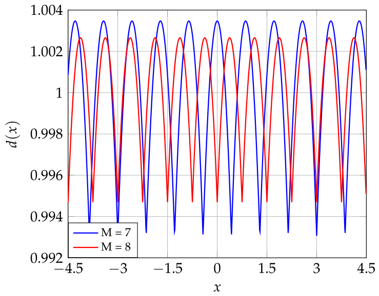
Figure 2.
Curves of (40) for , , and truncated Gaussian shaping with .
Figure 2.
Curves of (40) for , , and truncated Gaussian shaping with .
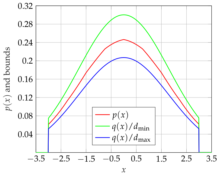
Figure 3.
for , , , , Gaussian and . Observe that is symmetric and periodic with period and in .
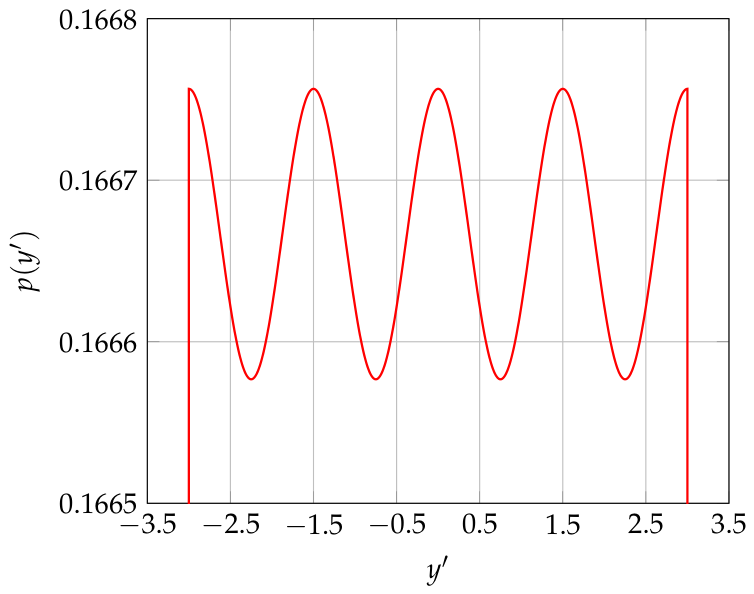
Figure 4.
and bounds for , , and truncated Gaussian shaping.
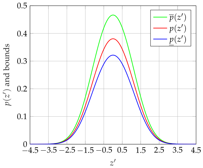
Figure 5.
Capacity and LP rate regions for the channels (69) with , and .
Figure 5.
Capacity and LP rate regions for the channels (69) with , and .
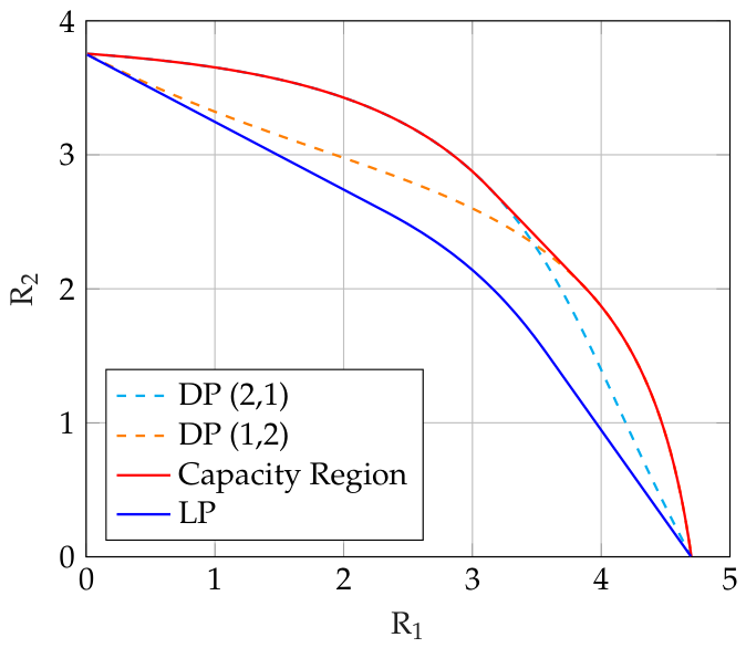
Figure 7.
Polar encoding for .
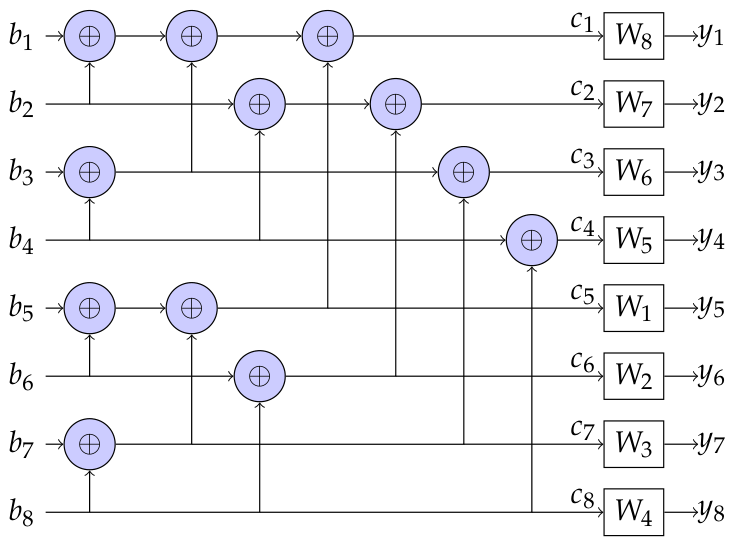
Figure 8.
FER vs. SNR for DPC and coded LP with multi-level polar codes. The code parameters are optimized at 11 dB.
Figure 8.
FER vs. SNR for DPC and coded LP with multi-level polar codes. The code parameters are optimized at 11 dB.
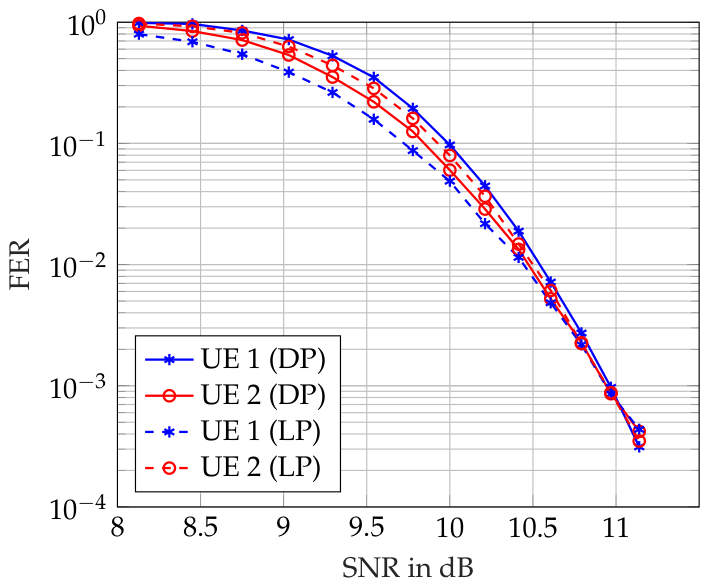

Table 1.
Simulation Parameters.
| sub | ||||||||||
| DP | UE 1 | 1 | 0 | 0 | 0 | 55 | 0 | 5 | 97 | 73 |
| no modulo | 2 | 0 | 0 | 10 | 110 | 3 | 52 | 117 | 12 | |
| UE 2 | 1 | 0 | 0 | 55 | - | 0 | 35 | 68 | - | |
| modulo | 2 | 0 | 10 | 110 | - | 6 | 88 | 12 | - | |
| LP | UE 1 | 1 | 0 | 0 | 55 | - | 0 | 61 | 72 | - |
| no modulo | 2 | 0 | 10 | 110 | - | 18 | 107 | 12 | - | |
| UE 2 | 1 | 0 | 0 | 55 | - | 0 | 34 | 67 | - | |
| no modulo | 2 | 0 | 10 | 110 | - | 5 | 86 | 12 | - |
Disclaimer/Publisher’s Note: The statements, opinions and data contained in all publications are solely those of the individual author(s) and contributor(s) and not of MDPI and/or the editor(s). MDPI and/or the editor(s) disclaim responsibility for any injury to people or property resulting from any ideas, methods, instructions or products referred to in the content. |
© 2026 by the authors. Licensee MDPI, Basel, Switzerland. This article is an open access article distributed under the terms and conditions of the Creative Commons Attribution (CC BY) license (http://creativecommons.org/licenses/by/4.0/).
Copyright: This open access article is published under a Creative Commons CC BY 4.0 license, which permit the free download, distribution, and reuse, provided that the author and preprint are cited in any reuse.