
Submitted:
14 May 2026
Posted:
14 May 2026
You are already at the latest version
Abstract
The efficiency of data-driven research relies not only on high-quality data and sufficient computational resources but also depends sensitively on the personal knowledge management of the researcher. The multitude of digital artefacts created during the researcher’s daily workflow might comprise experimental results, simulation results, literate programming notebooks analysing experiments and simulations, statistical models, machine learning models, figures, tables, and conversations with generative artificial intelligence systems. In order to trace and track these interconnected research artefacts over several months of research or even extended research periods and different research projects, these artefacts need to be systematically named so that they can be referenced in note-keeping systems and research outputs. Therefore, the naming and referencing scheme for research artefacts needs to be flexible, consistent, efficient and support the linking of artefacts across different software frameworks and even classical laboratory notebooks. This article introduces a hierarchical naming scheme and the supporting open-source Python package contexere together with best practises for the personal knowledge management for postgraduate students and early career researchers, which provides a clear and linkable structure for data artefacts and thus supports effective personalised research workflows.
Keywords:
reproducible research
; personal knowledge management
; postgraduate students
; earyl career researchers
1. Introduction
Note-taking systems are at the heart of every research project. Based on the research discipline, these note-taking systems might be referred to as laboratory notebook [1], engineering logbook [2], or just journal [3] (p. 108f). These systems might be manual or digital, with implementations ranging from notebooks and loose-leaf collections of printouts to digital text documents in the local file system, cloud-based services, and special-purpose electronic laboratory notebooks. In many cases, it will even be a mix of all or some of these elements.
Driven by the complexity of research workflows due to the incorporation of computational resources, the classical laboratory notebook [1,4,5] has become a niche documentation system, and the reproducibility of research has faltered to some extent over the last thirty years. Consequently, the topic of reproducibility has gained much traction, ranging from electronic laboratory notebooks [6], specific rules [7] to best practices [8,9]. Notably, these rules and best practises emphasize the usefulness of naming schemes to document the workflow process and connect data to plots and quantitative results to research statements. However, while previous attempts at establishing naming schemes [10] focused on connecting notes from classical laboratory notesbooks with computational resources, the required linking of research artefacts through different, continuously changing computational processing steps was missing or ineffective due to nomenclature overhead.
The goal of this work is to equip postgraduate students and early-career researchers with a starting point for building their research expertise and developing a personal knowledge management system, without overburdening them with complex and restrictive electronic laboratory notebooks. The general idea is that the file system on the researcher’s workstation or in cloud storage is sufficient to build a robust and flexible research management system that can be combined with existing frameworks for reproducible research and domain-specific laboratory notebook implementations. Therefore, this work addresses the need for a simple, consistent, and linkable naming scheme explicitely designed for postgraduate students and early career researchers. This approach builds on the Dreyfus model of skill acquisition [11] and accounts for the fact that beginners need clear rules success. Of course, the naming scheme can also be useful to established researchers. However, these scientists and engineers typically have developed effective methods for managing their data artefacts and research workflow, or they have switched to more high-level activities of senior researchers. They might still find inspiration in the presented workflows, or consider suggesting the methodology to their postgraduate students and mentees.
Note that in practice, the following suggestions and ideas should be combined with established best practices for reproducible research, such as data carpentry [8,9]. However, for reasons of simplicity and to emphasize that the suggested file naming scheme can be combined with most established frameworks for reproducible research, this article cuts to the core of this contribution. The following sections introduce a motivation for reproducible research, the file naming scheme, discuss several different workflows, and introduce software tools that support the usage of the naming scheme. The article concludes with a discussion and outlook.
2. The Directed Graph of Research Artefacts
The pinnacle of every research effort is the presentation and sharing of research findings. These reports might have the form of a presentation to a supervisor or a seminar, a formally written thesis, or a manuscript for a journal or a conference. Whatever the medium or occasion of sharing research results is, in the following, all these different forms of dissemination will be referred to as research reports.
A research report draws from the collection of the researcher’s insights and observations, which are supported by a range of research artefacts. Many of these research artefacts will be figures, diagrams, tables, or notes (Figure 1) with the intention of explaining a research problem, stating a hypothesis, describing an experimental setup, or deducing a theoretical framework, together with findings and conclusions. In this context, a research artefact can be characterised as follows:
- RA1
- A research artefact is a non-trivial, documented research output that contributes to a specific research project.
- RA2
- A research artefact is generated through the concentrated, creative work of a research activity with the intention to create new knowledge or insights.
- RA3
- A research artefact is typically embedded into the context of related research artefacts, which are either generated in the course of the same research activity or contribute to the artefact’s generation as input.
- RA4
- Research artefacts, which stem from the same research activity, form a Research Artefact Group (RAG).
These four characteristics RA1–RA4 of research artefacts require some more detailed explanations, which will be given in the following paragraphs after introducing an example (Figure 1).
An illustrative example of six research artefacts from two different research projects that contribute to a research report is shown in Figure 1. In this example, the two research projects are referenced as ERP and RRP, which stand for Example Research Project and Related Research Project, respectively. The example report contains four figures and one table from ERP and one figure from RRP as reflected in the filenames of the figures and tables included in the LATEX report. The filenames of the research artefacts not only reference the respective research projects but also the research activities or research artefact groups (RAG) via their unique identifiers. The convention for constructing the unique RAG identifiers will be defined later (Section 3), but just looking at the filenames of research artefacts in Figure 1 that contribute to the research report reveals a directed graph of dependencies, which allows for complete reproducibility.
The directed graph in Figure 1 also provides some examples of research artefacts. First of all, there are the directly visible research artefacts that prominently contribute to the report: the table (a stylised grid of scribbles) and the five figures (yellow, red, green, purple, and orange blobs). These research artefacts are definitely non-trivial (RA1) because they combine several aspects of the research question to support the report’s narrative in a meaningful way. Also, these artefacts have been generated through concentrated, creative work (RA2), as the researcher will have spent significant time collecting input data, designing the graph or table layout, tweaking annotations, and writing the figure and table captions. Most likely, these artefacts will have gone through several iterations before the final report is handed in.
The characteristics RA1 and RA2 determine the details of differentiating between research activities, while the interpretation of non-trivial and concentrated, creative work is project-specific and most likely will change throughout the project. E.g., writing the configuration files for a complex simulation is definitely a concentrated, creative task (RA2). If a specific simulation setup is run with dozens or more parameter variations in the course of a systematic parameter sweep or hyperparameter optimisation, the individual simulation output becomes trivial because it contributes only a datum to the respective analysis task. However, setting up the sequence of systematic parameter variations is concentrated and creative work (RA2) and the collected data of this task are non-trivial (RA1).
The visible research artefacts of a research report typically do not stand alone but are embedded in a context of other research artefacts (RA3), such as Python, R, or shell scripts, as well as configuration files for simulation frameworks and processed and raw data, to name just a few. E.g. the stylised green figure named ERP26pNc__fig_green.png in Figure 1 has been generated via a literature programming approach [12] via a Jupyter notebook (ERP26pNc__fig_green.ipynb) visualising some input data (ERP26pNc__exp_x=30.csv). These three files form a research artefact group (RAG) because they share the context of the same research activity (RA4), namely, analysing and visualising the data encoded in a specific CSV file. Note that these three file names start with the same RAG identifier (ERP26pNc), which groups them within a specific artefact group. The rules for constructing the identifier will be detailed in Section 3. However, in order to indicate the information density of the chosen identifier, it is remarked that ERP26pNc references project ERP, the date of creation 26pN, namely the 23 February 2026, and the fact that it is resulting from the third (c) research activity of this day.
The linking of RAGs is demonstrated in Figure 1 for the yellow RAG labelled ERP26pNd_a_Lc_oVc. This RAG contains Python script ERP26pNd_a_Lc_oVb__analysis.py and produces a Portable Network Graphics file ERP26pNd__barplot.png and a table ERP26pNd__table.tex already encoded in LATEX, e.g. by using the convenient method .to_latex() provided by DataFrame objects [13,14]. While the RAG identifier is clearly ERP26pNd, the trailing, underscore-separated groups “_a_Lc_oVb” indicate that some kind of input is used from RAGs ERP26pNa, ERP26pLc, and ERP26oVb. In anticipation of Section 3, it is remarked that links between RAGs are created by the least significant elements of RAG identifiers compared to the root RAG identifier. In the given example of ERP26pNd_a_Lc_oVb, the input might be summary statistics contributing to the barplot of ERP26pNd, which are computed from
- ERP26pNa__exp_x=10.csv.
- ERP26pLc__exp_x=30.csv,
- ERP26oVb__exp_x=20.csv,
Of course, the researcher will know and remember, in the course of writing the report, how the different RAGs are connected. However, in the context of knowledge management, it is well known that the knowledge of an individual is subject to forgetting [15]. By explicitly encoding the dependencies of research artefacts into their filenames, a directed graph of research artefact dependencies is generated, which might become relevant for a future higher-level report (e.g., a thesis) when several older reports are collated into a more comprehensive document. Another scenario might be that future research reveals a flaw in the data acquisition or the configuration of a specific experiment, resulting in a compromised research artefact, so that all research artefacts that depend on the flawed RAG must be tracked down and updated.
3. Chronologically Referenced Research Artefact Groups
As demonstrated in the oversimplified example in the previous section, research artefacts, such as digital files or analogue notes, are grouped according to the research activity that generated them. In a typical researcher-led project, the creative parts of these research activities naturally separate the different groups along the daily work stream, so that the research artefact groups (RAGs) can be effectively named using a chronologically referenced scheme.
3.1. Requirements
Given the fact that the naming scheme has to support the ongoing and consistent naming of digital research artefacts, the following requirements can be formulated for the naming scheme:
- Chronological:
- The naming scheme encodes the date and sequence of research artefact groups such that the link to handwritten entries in laboratory notebooks is given.
- Lexiographic:
- The naming scheme is designed such that alphabetical sorting generates the chronological order in which research artefact groups were generated.
- Linkable:
- The naming scheme supports the linking of connected research artefacts, such that the research can easily identify data provenance.
- Unique:
- The naming scheme generates unique identifiers, such that the researcher can reference the research artefact in a note-taking system.
- Efficient:
- The naming scheme is efficient such that the researcher has to type as few characters as possible.
Applying the CLLUE principle (chronological, lexicographic, linkable, unique, efficient) to the naming of research artefact groups improves the daily research workflow on several different time-scales:
- In the rush of daily research, it provides simple rules for naming digital files and indexing handwritten notes with the additional benefit that connected research outputs are naturally linked.
- On the weekly time-scale, the embedded temporal reference of the naming scheme supports the personal review [16] of research progress and the planning of next steps.
- On the monthly time-scale of producing reports, presentations, and publications, the naming scheme links figures and tables to the originating research outputs.
- On the yearly-time scale of generating higher-level research outputs like theses or research proposals, the required figures can be easily identified from previous research outputs, adapted, and linked to the original research artefact.
- On the three to five year time-scale of building a research group, supervised students can be easily equipped with previous research outputs and thus get a head-start in their own research.
The following section formally defines the naming scheme for RAGs, including their linking.
3.2. Naming Scheme
In contrast to previous attempts to introduce naming conventions for research artefacts [10], which used ISO 8601 [17] to encode the temporal relations among research artefacts, the suggested naming scheme aims for efficiency and the ability to naturally track research progress and dependencies among research artefact groups.
The scheme for the identifiers of research artefact groups is PIyymDc[_link[_link]]:
- PI
- is the project identifier [a-zA-Z]{2,} consisting of at least two letters.
- yy
- m
- is one of the letters [o-z] encoding the month (left columns in Table 1). The month sequence [o-z] starts with the letter o because the twelve letters opqrstuvwxyz avoid the letter l, which can be easily confused with the digit 1 for some fonts.
- D
- is one of the ASCII characters [1-9,A-V] encoding the calendar day (columns 3–6 in Table 1). Digits 1 to 9 encode the first nine days of each month and characters A to V days 11 to 31. Digits and uppercase characters have approximately the same height, giving this element a visual structure to the RAG identifier and dividing the date from the daily counter.
- c
- is one of the lower case letters [a-z] encoding a daily counter of research artefact groups in alphabetical order. Realistically, a typical workday won’t have more than 26 distinct non-trivial research activities. Otherwise, there are strong indications that several closely related research activities should be grouped.
- link
- is an optional abbreviation of a predecessor RAG identifier indicating that the predecessor RAG contributes to the current RAG. The predecessor RAG identifier is abbreviated by showing only its last significant ASCII characters, which differ from the current RAG identifier. A list of links is separated by underscores, with the abbreviated RAG identifiers being listed in achronological order.
Having the naming convention formally be defined, the RAG identifiers of the illustration in Figure 1 can now be manually decoded into the achronological order of the respective activities (Table 2).
In addition, the LATEX-document of the research report Report26pNa__contexere.tex (top box in Figure 1) has been chronologically indexed with an RAG identifier (26pNa) indicating the first version of this document generated on 2026-02-23. In general, it is advised to use classical revision control [19] for LATEX-documents. However, the RAG identifier might come in handy for clearly indicating when work on this document started and for tracking major versions over the period of writing. This application of RAG identifiers is even more handy for binary document files like .docx or .pptx in combination with RAG linking to indicate document inheritance.
3.3. Linking Research Artefact Groups
The linking of research artefact groups has already been indicated in the illustration of Figure 1 and the definition of the RAG naming scheme in the previous section. The central idea is that RAGs that directly contribute to the head RAG are explicitly referenced in the RAG identifier as a list of abbreviations. However, not more than three RAGs should be listed in the filename to diminish readability. Dependencies to more than three predecessor RAGs indicate a systematic experiment, where the RAGs should be referenced in a tabular data file.
The illustration in Figure 2a shows the decoding of linked RAGs over different time-scales and even across projects. The linked RAG ERP26q3a was created on the same day, just before the work on RAG ERP26q3b started. RAG ERP26q2c was created on the previous day, RAG ERP26pVa was created in the previous month, and RAG ERP25zAb was created the previous year. The last RAG RRP25z1b contributing to ERP26q3b cross references a different project. Naturally, most links to predecessor RAGs will consist of one or two characters that reference the same-day or previous-day research activity. References across months (three characters) or calendar years (five characters) are typically found at the beginning of calendar months.
The linking of RAGs extends beyond digital files to handwritten notes, as demonstrated by Figure 2b, which shows a notebook excerpt with the concept study for the illustration in Figure 2b. The notebook shows both the date in day-month-year format (top right) and the RAG KM26q3a (top left) of this brainstorming session, which is referenced in the filename of the final artwork (KM26q3b_a). Therefore, the filename links the illustration to the respective handwritten notes.
4. Research Workflows Using the Naming Scheme
The following workflows build upon the best practises for reproducible research [9] while adding the naming scheme to generate a directed graph of research artefacts. The workflows build upon the open-source Python project contexere2, which provides helpful tools for using the proposed naming scheme. The contexere Python package provides the command line tool nxt pronounced next (Figure 3), which can be installed from PyPi3 for Python version 3.10 and above with the command:
pip install contexere
The following sections describe useful research workflows that embed the contexere implementation of the proposed naming scheme to increase productivity and enhance reproducibility. The following examples have been generated on macOS Tahoe 26.4 with the Anaconda Python distribution4 version 25.5.1. A basic Python compiler on Windows or Linux systems will generate similar results.
4.1. Starting a New Research Project
Starting a new research project means different things in different disciplines and contexts. A common denominator is the requirement for a filing system or directory structure that distinguishes raw and derived data, project-specific source code, literature programming notebooks (e.g., R Markdown or Jupyter notebooks), figures, notes, and reports. With the support of the contexere package, the following three steps will set up a basic directory structure and templates (Section 4.1.1), initialise revision control (Section 4.1.2), and create a virtual Python environment (Section 4.1.3):
- Create folder structure: $
- nxt --project # dialog sets variable repo_name
- Change into new project folder: $
- cdrepo_name
- Init revision control: $
- git init; git add .; git commit -m ’Initial commit’
- Create virtual environment: $
- make create_environment
The following sections explain the automatic generation of the project folder structure (Section 4.1.1), the initialisation of revision control (Section 4.1.2), and the creation and usage of the virtual Python environment (Section 4.1.3).
4.1.1. Folder Structure
The folder structure proposed for a typical data-driven research project builds upon best practises [9] (p 11) and has been amended from the project template provided by the Cookiecutter Data Science project [20]. The proposed folder structure can be initialised with the shell command
nxt --project
which starts a dialogue allowing the user to configure the project template accordingly.
An example dialogue is shown in Figure 4a. The first question asks for a short, meaningful project title. In this example, the project title Example Research Project was chosen, which already appeared in the previous section. Based on the project title, the dialogue suggests two abbreviations: The first abbreviation is the repository name (repo_name), which, by default, is built from the first letters of the title words. In this example, the abbreviation ERP will be used as the name for the project folder and the project-specific virtual Python environment. The second abbreviation (module_name) will be used to set up the code scaffold for a project-specific Python module and, by convention, should only contain lowercase letters. By default, module_name is derived from repo_name by converting all letters to lower case. In the dialogue shown in Figure 4, the suggestion erp is accepted. The dialog in Figure 4 continues with questions about
- the project description,
- the author’s or organisation’s name,
- the Python version for the virtual environment,
- the Python environment manager,
- the preferred file for defining package dependencies,
- the configuration of a unit-testing framework,
- the support packages for linting and formatting,
- the license template, and
- the documentation framework.
Finally, the user can choose to generate a project-specific code scaffold for a standalone Python package, which is useful for refactoring functions and classes from tracer-bullet development [21] in Jupyter notebooks to reusable Python modules.
Using the information from the command line dialogue, a directory ERP is generated (Figure 4b), which holds the required files and folders for a data-driven research project. The directory structure (Figure 4b) features a data folder, which discriminates between data from third party sources (external), immutable input data (raw), an intermediate data stage after initial transformations (interim), and a folder for the data after preprocessing has been completed (processed). For many applications, the required data will be too large to be revision-controlled (Section 4.1.2), and the respective folders should be manually replaced with symbolic links to research or cloud storage drives.
The docs folder combines project-specific documentation provided in Markdown files with documentation extracted from Python doc-strings. Using these mechanisms requires installing a virtual Python environment, as explained in Section 4.1.3. The configuration file environment.yml has been preconfigured to manage the dependencies on other Python packages, as requested during the configuration dialogue. It accounts for the optional installation of PyData packages and the project-specific Python package, erp in this example. The code scaffold for the erp package is provided in the erp folder as a standalone project-specific Python package, which can be imported after installing the virtual environment (Section 4.1.3).
The LICENSE file is only provided if either the MIT12 or BSD-3-Clause13 has been chosen in the dialogue. A discussion and comparison of these open source license families can be found in [22].
The Makefile is discussed in greater detail in Section 4.1.3. Its main purpose is to automate certain project tasks, such as installing a virtual Python environment or preprocessing a dataset, as defined in erp/dataset.py. The notebooks folder holds Jupyter notebooks [23] (Chapter 3) and is populated with a template notebook, which has a preconfigured Python header for importing the most important PyData packages (Figure 5a). The template notebook header changes depending on the user’s choice of the pydata_packages option. Choosing option basic imports the respective Python libraries and module-specific savefig function (Figure 5a), which is discussed in Section 4.4. Choosing option none in the user dialogue omits the PyData packages from the notebook header (Figure 5b). Also, the module-specific savefig function is omitted, because it depends in its default configuration on matplotlib. Typically, the template notebook can be cloned at the beginning of a session, and the resulting notebook is renamed according to the proposed naming scheme (Section 3).
The pyproject.toml file implements the requirements for building the project-specific Python package [24]. It is preconfigured based on information during the user dialogue. The Markdown file README.md uses information like project_name, author_name, and description to provide a project overview. The file README.md is typically the first impression for a potential user if a project is published on developer platforms like GitHub14, Bitbucket15, or GitLab16.
The references folder contains project support information like, such as literature, bibliographies, or specification documents. An example is the reference sheet of Table 1 provided as reference/figs/KM26oOa__contexere_dates.png. The reports folder contains project summaries and research outputs, such as presentations or manuscripts intended for external audiences. It holds a template report that includes LATEX code to embed figures from the ERP/results/figs and ERP/reference/figs folders, and compiles a bibliography from ERP/references/ERP_bibliography.bib.
The results folder and its contents document the project’s progress by capturing intermediate research results, which should always be paraphrased and summarised in a logbook or diary file [9]. Here, the Org Mode17 file ERP_logbook.org (highlighted at the bottom of Figure 4b) is preconfigured with information from the initialisation dialog and a first entry with RAG ERP26s6a documenting the date of project initialisation (6 May 2026) while using the proposed naming scheme to reference the respective research artefact named ERP26s6a__directory_structure.txt. Org Mode files are a Markdown variant combining task and project management with literate programming [12,25], LATEX-support, encryption support, mobile applications18, and many other features integrated into GNU Emacs19. In combination with Git (Section 4.1.2), Org Mode files have demonstrated their usefulness for supporting research workflows and documenting research results [26].
4.1.2. Revision Control
Revision control is a software engineering methodology that tracks changes and edits to a software project over time, supporting distributed development and backups. For software-based research projects, revision control is extremely valuable because it allows reproducing in-silico experiments, naturally links software versions to logbook entries, and allows the recovery of unsuccessful refactoring attempts. The de facto standard for revision control is the open-source tool Git [19,27], which was initiated by Linus Torvalds as a revision control system for the Linux kernel. One of its key features is the fact that every local version of a Git repository is a complete copy of the repository’s history. This approach ensures fast local queries and provides inherent redundancy against accidental loss or corruption of data, if the local git repository is mirrored to a remote repository [19] (p. 110ff).
The following paragraphs assume that the Git tool is readily available on the researcher’s computer, either because it is delivered with the operating system or installed separately. Chacon and Straub [19] (p. 18ff) give detailed instructions on how to install a new or updated version of the Git tool for Linux, macOS, or Microsoft Windows systems.
The local Git repository is typically initialised by opening a command line shell (Figure 6), changing directory to the project folder (Section 4.1.1) and executing the following command:
git init
The next step is to add all files of the initialised project to the repository with the command
git add .
Note, the dot “.” following git add is part of the command. The process of adding new or changed files to the repository is called staging. In general, the command git add will not be used with a dot “.” as an argument but with specific file names, which are either new or have been edited. The reason is that compilation processes usually generate many helper files that change frequently but do not contribute to documentating the project’s history. These helper files can be excluded from staging suggestions by configuring the .gitignore file. However, because a project initialised with nxt --project starts with a project scaffold (Section 4.1.1) and does not have any data or large files yet, it is safe to initialise the local git repository using the dot-syntax.
A second step is required to add the staged files to the local repository. This process is called committing and requires a commit message, which explains why the change was necessary. A trivial but sensible commit message for the first commit might be:
git commit -m "Initial commit"
Now, the research progress can be documented with subsequent git add and git commit commands. The commit history can be inspected with the command git log (Figure 6), which shows a hexadecimal hash identifying the commit, the author and the author’s email address, commit date, and the commit message.
Note that a first-time git user will be prompted to configure the preferred username and email. This information is used to annotate every commit and to support workflows involving two or more researchers or software engineers. As can be seen from the bottom of Figure 6, the author had previously used the following commands to configure these variables:
git config –global user.name "Andreas W. Kempa-Liehr"
git config –global user.email "a.kempa-liehr@auckland.ac.nz"
Here, the option --global defines that the variables should be used for all git projects on the respective computer system. Omitting the --global option sets the variables just for the current git project.
With a newly initialised research git repository at hand, some more advanced revision control features can be used to document and track the research progress (cf. Section 4.2 and Section 4.3)
4.1.3. Virtual Python Environment
Based on the information provided during the command line dialogue (Figure 4a), a project-specific Makefile [28] is configured such that the command
make create_environment
generates a virtual Python environment named ERP. This name is the value of variable repo_name, which was assigned during the command line dialogue discussed in Section 4.1.1.
The make command is installed by default on most Linux distributions. On macOS, it can be installed via the Xcode Command Line Tools with xcode-select --install. On Microsoft Windows systems, the Software Distribution and Building Platform for Windows20 (MSYS2) supports the installation of GNU Make via
pacman -S make
After executing make create_environment and following the instructions for activating the newly created virtual Python environment, a project-specific Python module named with the value of variable module_name is available (Figure 4a), which can be imported into Python scripts and Jupyter notebooks with the usual Python command
importmodule_name
Based on the configuration for the example project, the module files are located in folder ERP/src/erp and the module can be loaded with import erp (Figure 7a) if erp was chosen by the researcher as input for variable module_name during the initialisation dialogue (Figure 4). The project-specific Python module will provide functions and classes, which be refactored [29] over time from Jupyter notebooks. In addition, important configuration variables, such as paths to the different data folders and the figures folder, can be loaded from the module erp.config (Figure 7a).
The virtual environment also provides all required Python packages to generate an interactive webbrowser-based project documentation (Figure 7c), which is preconfigured using the information provided in the project initialisation dialogue (Figure 4). As shown in Figure 7b, the documentation is build with
mkdocs build
and the local web server is started with
mkdocs serve
4.2. Tagging Repository Commits
Beyond the established revision control practises for software development [19], the command git tag can be integrated into reproducible research workflows using the proposed naming scheme. The general idea is to document certain stages of the research project using RAG tags, which reference specific commits in the git repository. E.g., the state of the repository related to logbook entry ERP26s6a (highlighted text at the bottom of Figure 4b) could be tagged by the command:
git tag ERP26s6a
The tag ERP26s6a is basically a bookmark for the commit hash
cc82bfa9aa6e9496de7ca652edda63c90d850e9d3
(cf bottom of Figure 6) and allows to recover the exact state of the repository at 6 May 2026 19:45:06 New Zealand Standard Time (+1200), because the respective commit included all the changed files up to this commit. From now on, the repository state associated with tag ERP26s6a can be recalled with
git switch --detach ERP26s6a
This command creates a so-called headless state of the repository, which can be used to inspect all files of this specific repository state, but files cannot be changed. After inspection, the command
git switch main
returns the repository to its latest working stage, because main is the default working branch of git repositories. Alternatively, a specific file of tag ERP26s6a like ERP_logbook.org can be shown with
git show ERP26s6a:results/ERP_logbook.org
More importantly, previous versions of files can be recovered with git restore. Let us assume that the README.md file needs to be rolled back to its original version of tag ERP26s6a, which can be achieved with
git restore --source=ERP26s6a -- README.md
Now, the file README.md has been changed to its version at tag ERP26s6a, which can be edited and committed in its restored or amended version to the repository:
git add README.md
git commit -m "Restored from ERP26s6a"
While this specific tagging example is admittedly overdone for the very first commit of a repository, the tagging of selected commits with associated RAGs takes into account that research software is never finished per se, but undergoes permanent development and enhancement, such that specific analysis or experimental results require the link to a specific repository commit in order to guarantee reproducibility.
4.3. The Naming Scheme in Practise
Some examples of using the nxt command in the context of the project structure generated in Section 4.1.1 are shown in Figure 8. Note that all of these examples have been created on 6 May 2026 (26s6) after the initialisation of the ERP project.
Calling the nxt command in an empty directory without any arguments returns the date abbreviation with the first step counter letter “a” appended (Figure 8a). Calling the nxt command at the root of a directory structure, which contains files following the RAG naming scheme, finds the latest RAG and uses the respective project identifier to suggest a new RAG (Figure 8b). The newly generated ERP project already has an RAG named ERP26s6a (right-hand side of Figure 4), such that the next RAG started on 6 May 2026 is ERP26s6b (Figure 8b). An overview of the existing files associated with RAGs gives the command
nxt --summary
which provides a tabular output of all RAGs (Figure 8c).
Up to this point, the nxt command has only been used to avoid the consultation of Table 1 and the manual counting of RAG steps. However, let us assume we want to start a new Jupyter notebook to develop a proof-of-concept (POC) that uses the template notebook as a starting point. A copy of the provided template ERP26s6a__template_notebook.ipynb can be generated with the command
nxt notebooks/ERP26s6a__template_notebook.ipynb --keywords poc
resulting in an exact copy of the template (Figure 8d) named with the next available RAG and the provided keyword:
notebooks/ERP26s6b__poc.ipynb
The cloned file is added automatically to the git repository of the project (Figure 8e) such that all edits can be tracked systematically.
Let us assume that we want to follow up with a visualisation of data or results generated by ERP26s6b__poc.ipynb. In this case, we might want to continue from the configuration provided in ERP26s6b__poc.ipynb. The command
nxt notebooks/ERP26s6b__poc.ipynb --reference --keywords visualisation
creates a copy of ERP26s6b__poc.ipynb in directory notebooks named
ERP26s6c_b__visualisation.ipynb
Note that the cloned RAG references the original RAG. In another rapid development cycle, we might want to continue from ERP26s6b, but this time using additional data from a completely different project, DS25zAa, where DS might stand for data science. The command
cd notebooks
nxt ERP26s6b__poc.ipynb --reference s6b,DS25zAa --keywords simulation
creates a fourth notebook named
ERP26s6d_b_DS25zAa__simulation.ipynb
again, providing efficient references to the input RAGs and thus creating a directed graph of RAGs. Note that the provided reference s6b is an abbreviation of ERP26s6b, which is shortened to the step counter “b” in the filename of the cloned notebook.
These examples demonstrate the enhanced automation of research documentation provided by the combination of the naming scheme and the nxt command.
4.4. Saving Figures with Metadata
In quantitative research, the researcher typically generates a multitude of plots and diagrams, of which only a fraction will be included in shared or published research outputs. However, the process of generating, interpreting, and documenting the visualisations guides the research, fosters communication with collaborators and supervisors, and supports the researcher’s review process and planning of next steps.
While the cloning of scripts and notebooks discussed in Section 4.3 guarantees that all scripts and notebooks are labelled with a valid RAG identifier, the saving and documentation of derived research artefacts like data or figure files requires that the respective filenames start with the RAG identifier of the generating program (Figure 1). In order to support the automated naming of generated files and foster the generation of scripted analytics reports, the function artefact_name() provided by the contexere package retrieves the RAG of the respective Python script or Jupyter notebook and appends keywords for documentation purposes. The example shown in Figure 9a is a screenshot of a Jupyter notebook
ERP26s6b__poc.ipynb
Calling the function artefact_name() in this notebook (Cell [2] in Figure 9a) returns ERP26s6b, which is the notebook’s RAG identifier. The function had returned the same output ERP26s6b if it had been called from a Python script named ERP26s6b__*.py.
Cell [6] of the notebook generates a histogram and stores the plot using the savefig() function, which was imported from the project-specific module erp.plots in Cell [1] (Figure 9a). The savefig() function is preconfigured such that all figures are stored in the results/figs folder of the standardised project structure (Figure 4b) (Cell [8] in Figure 9a). By default, savefig() generates Portable Document Format (PDF) files, but also supports Portable Network Graphics (PNG) and Scalable Vector Graphics (SVG) if the suffix option is configured or the first argument of savefig() ends with .png or .svg.
The restriction to the three graphic formats PDF, PNG, and SVG is deliberate to support the storage of additional metadata, such as author, title, and the creating application, in the generated files. Figure 9b shows the Document Properties windows of Adobe Acrobat (Version 2026.001.21367) for the generated file ERP26s6b__histogram.pdf. The metadata for PNG images can be checked with the .info attribute of the Python object created by loading the PNG images with PIL.Image.open(). Because SVG images are based on the Extensible Markup Language (XML), they can be opened with any text editor, and their metadata is stored in the SVG file header.
4.5. Logbooks and Reports
Markup languages like Markdown, Org Mode, or LATEX are convenient for maintaining an overarching documentation of research progress over longer periods of time. These markup languages seamlessly integrate with the revision control systems used in research projects, and images and smaller result tables can be directly embedded in these documents.
Two different Markup examples are shown in panels (a) and (b) of Figure 10. Panel (a) shows the extended logbook ERP/results/ERP_loogbook.org introduced during the project setup (Figure 4b, bottom). Lines 10 and 11 of Figure 10 integrate the PDF image ERP26s6b_histogram.pdf created in the previous section into the Org Mode document:
- 10
- #+ATTR_LATEX: :width 0.4\textwidth
- 11
- [[file:./figs/ERP26s6b__histogram.pdf]]
Line 11 specifies the figure’s path, and line 10 configures its display for the LATEX export, as shown in the compiled PDF version of Figure 10c. The PDF is generated in Emacs by the four key strokes
CTRL-c CTRL-e l p
or short C-c C-e l p. Note that the double brackets in line 11 of the Org Mode source code shown above are hidden in the screenshot of Figure 10a because Emacs converts the reference to the PDF image into a clickable link, which opens the respective PDF image.
The second markup example is a LATEX file, generated by cloning and editing the provided report template ERP/reports/ERP26s6a_example_report.tex. This example was chosen to demonstrate the usage of the \copyrightbox macro (lines 12–15 in Figure 10b), which has been used to reference the filename of the displayed image at the right-hand side of the image:
- 12
- \copyrightbox{
- 13
- \includegraphics[width=\textwidth]{ERP26s6b__histogram.pdf}
- 14
- }
- 15
- {\texttt{ERP26s6b\_\_histogram.pdf}}
Note that the underscores of the filename have to be escaped (line 15). A screenshot of the respective PDF is shown in panel (d) of Figure 10.
The convenient file link in the Org Mode document (Figure 10a) does not show the filename on the figure’s right-hand side (Figure 10c). This deficit can be circumvented by inserting a LATEX-header configuration into line 3 of the Org Mode document
- 3
- \texttt{#+LATEX_HEADER: \usepackage{copyrightbox}
and placing the \copyrightbox inside an Export block such that lines 10 and 11 of Figure 10a are replaced by
- 10
- #+BEGIN_EXPORT latex
- 11
- \copyrightbox{
- 12
- \includegraphics[width=0.4\textwidth]{ERP26s6b__histogram.pdf}
- 13
- }
- 14
- {\texttt{ERP26s6b\_\_histogram.pdf}}
- 15
- #+END_EXPORT
While markup languages always provide a direct link to the respective filenames in their source code, the additional references to filenames in the compiled PDF create additional links between notes and RAGs, which simplifies the researcher’s review process.
5. Working with Generative Artificial Intelligence
5.1. Case Study
Working with generative Artificial Intelligence (AI) has quickly advanced from a toy application to a productive research assistant [30]. This capability means that a researcher can easily generate introductory material, potential solution strategies for coding problems [31], up to literature review drafts [32]. In the context of a research project, these conversations with generative AI services must be considered research artefacts that may be useful for advancing the research project. Nevertheless, reproducibility requires that all information sources are documented and can be queried afterwards. While all publicly available generative AI services have some chat history, which allows revisiting past conversations, a researcher quickly ends up with multiple wordy research artefacts distributed across different websites and services. In addition, most conversations with generative AI will not be exactly repeatable, as with a colleague, because the model and the AI agent’s state are likely to change unknowingly in the background. The solution is to extract the conversations into a local note-taking system and index the resulting research artefact within the research context. This approach enables the researcher to clearly document which information was retrieved from generative AI and differentiate this input from own derivations, source code, and inventions. The documentation of input retrieved from generative AI will also help justify statements about the extent of generative AI use, which is required by many publishers at the submission time of journal manuscripts.
The following case study outlines strategies for exporting answers from generative AI chatbots into a personal knowledge management system while documenting the information retrieval process. The question, which was presented to the generative AI chatbots, is closely related to the contexere package and should clarify if the introduction of a command line argument next would create any confusion with established tools:
In the context of Unix or Windows based terminals, are there any commands, utilities, programs, or executables named “next”?
The question was prompted on 5th February 2026 (26p5) to Copilot, Grok, Gemini, and Claude (Table 3). The short answer is that there are no system or shell commands named “next” in Unix or Windows-based operating systems, but the web framework Next.js provides a next command, which would collide with a similarly named tool provided by the contexere package.
5.2. Copilot
Copilot is integrated into the Microsoft 365 cloud services. Therefore, it is not surprising that the best export option is Microsoft Word documents. Individual answers can be exported to .docx documents by clicking the …-menu below the answer and choosing Export to Word. The exported document is saved in the user’s OneDrive or SharePoint cloud storage, and the exported file is named after the prompted question. Therefore, the first step is to locate the exported file in OneDrive or SharePoint, and rename the .docx file using the proposed naming scheme. Then, the Copilot prompt needs to be manually added to the exported .docx document by copying and pasting the prompt from the chat window. After this edit, the document can be downloaded to the results folder of the local research repository. Using the commands git add, git commit, and git tag, the respective file can be added to the research repository. These git commands must be repeated for all newly generated files and will be regarded as a matter of course for the following steps.
For this specific experiment, the name of the downloaded .docx file was
KM26p5b__Copilot_next_command.docx
indicating the second (“b”) RAG of the KM project on 5 February 2026. In the context of this RAG, a screenshot of the Copilot window next to the Microsoft Word window was taken, which was named with the same file stem:
KM26p5b__Copilot_next_command.png
The screenshot was manually redacted and presented as
KM26p5c_b__Copilot_redacted_screenshot.png
in Figure 11a. The additional documentation in the respective Org Mode logbook of the project was
- $ git show KM26p5c | tail -n 38 | head -n 18
- +*** Copilot (Fig~\ref{fig:KM26p5c})
- +- Rename Chat to reference RAG
- +- Below the answer open the ~More options~ $\ldots$ menu choose ~Open in Word~
- +- Rename Word file to reference RAG
- +- Copy Question into the Word document
- +- This export has to be reported for every question, such that a complete conversation has to be collated manually.
- +
- +#+BEGIN_EXPORT latex
- +\begin{figure}[H]
- +\begin{center}
- +\copyrightbox[b]{
- +\includegraphics[width=\textwidth]{KM26p5c_b__Copilot_redacted_screenshot.png}
- +}{KM26p5c\_b\_\_Copilot\_redacted\_screenshot.png}
- +\end{center}
- +\caption{Screenshot of Copilot conversation and DOCX export. Note, that the question is missing in the export.}
- +\label{fig:KM26p5c}
- +\end{figure}
- +#+END_EXPORT
As shown in these notes and the screenshot in Figure 11a, the prompt was not copied into the exported document at the time the screenshot was taken. Also, the notes indicate that either the chat needs to be renamed before export, or the exported Word file needs to renamed after export.
5.3. Grok, Gemini, and Claude
The export processes for conversations with Grok, Gemini, and Claude (Table 3) are slightly different to the one described for Copilot. The main difference is that at the time of writing, Grok, Gemini, and Claude feature reliable export functions to Markup formats and include the input prompt in the exported file. E.g., Org Mode exports can be generated by prompting
Convert this conversation to orgmode.
Example screenshots from Grok are shown in Figure 11b. The same instructions usually work well for Markdown and LaTeX. Figure 12a shows the conversation with Gemini on the left and the exported Markdown file rendered by Obsidian22 on the right-handside.
In addition, Claude features a robust conversion to PDF with the prompt:
Download this conversation to PDF.
For this chatbot, the generated PDF is directly visualised in the chatbot window (Figure 12b).
In any case, the researcher must manually rename the resulting export files to match the intended RAG, ensuring the filenames correspond to the notes in the researcher’s logbook. For complex answers involving formulas and tables, the researcher should always check the exported conversations for completeness and, if the export is incomplete, either print a PDF directly from the browser window or take screenshots. After that, the evaluation process of checking the chatbot’s outputs against hallucinations can be documented in the researcher’s logbook.
6. Discussion and Conclusions
A researcher’s personal knowledge management system is always a highly personal, individualised implementation of note-taking and evidence-collecting processes. However, given the huge productivity increase in research fostered by information and communication technology and the evolving adoption of generative AI chatbots, new documentation processes need to be developed and implemented that allow the systematic referencing and linking of different types of research artefacts.
The suggested naming scheme has evolved over 30 years, starting with the author’s diploma thesis, and a previous iteration was published in [10], wich still relied on the ISO date format. Several iterations later, and after about five years without changing the naming scheme, the key inside is still that related research artefacts are typically generated in groups of files or notes across different media. Research artefacts are always generated as the results of a non-trivial research effort. Moreover, the key reference point for theis fragmented information is the time when work on a specific research task began. Therefore, minor edits should always be applied without changing the RAG if the context has not changed, because revision control guarantees that all previous versions of scripts and figures are preserved. Linking RAGs via a systematic naming scheme, combined with an individualised note-taking system, provides a flexible methodology for linking research artefacts to research notes across short- and long-term research periods and diverse research projects.
Taking these very general requirements into account, the suggested naming scheme provides a chronological, lexicographic, linkable, unique, and efficient identifier for documenting research progress. Because the naming scheme is published together with an in-depth example implementation of a research workflow based on the open-source Python implementation contexere package, In conclusion, the described principles and suggestions will be very useful for enhancing the research efficiency of postgraduate students and early-career researchers.
Funding
This research received no external funding.
Data Availability Statement
The contexere Python package is available at https://github.com/kempa-liehr/contexere.
Acknowledgments
The author would like to thank A. Jeremiah and J. Greenwood for the testing of the contexere package.
Conflicts of Interest
The authors declare no conflicts of interest.
Abbreviations
The following abbreviations are used in this manuscript:
| AI | Artificial Intelligence |
| DS | Data Science |
| CLLUE | Chronological, Lexicographic, Linkable, Unique, Efficient |
| ERP | Example Research Project |
| ISO | International Organization for Standardization |
| KM | Knowledge Management |
| MSYS2 | Software Distribution and Building Platform for Windows |
| Portable Document Format | |
| PNG | Portable Network Graphics |
| POC | Proof Of Concept |
| RAG | Research Artefact Group |
| RRP | Related Research Project |
| SVG | Scalable Vector Graphics |
| XML | Extensible Markup Language |
References
- Thomson, J.A. How to Start–and Keep–a Laboratory Notebook: Policy and Practical Guidelines. In Intellectual Property Management in Health and Agricultural Innovation: a handbook of best practices: Volume 2; Krattiger, A., Mahoney, R.T., Nelsen, L., Thomson, J.A., Bennett, A.B., Satyanarayana, K., Graff, G.D., Fernandez, C., Kowalski, S.P., Eds.; MIHR and PIPRA, 2007; Volume chapter 8.2, pp. 763–771. [Google Scholar]
- McAlpine, H.; Cash, P.; Hicks, B. The role of logbooks as mediators of engineering design work. Des. Stud. 2017, 48, 1–19. [Google Scholar] [CrossRef]
- Hunt, A. Pragmatic thinking and learning: refactor your "wetware"; Pragmatic: Raleigh (North Carolina), 2008. [Google Scholar]
- Kanare, H.M. Writing the laboratory notebook; American Chemical Society: Washington, D.C., 1985. [Google Scholar]
- Ebel, H.F.; Bliefert, C.; Greulich, W. Schreiben und Publizieren in den Naturwissenschaften, 5th ed.; Wiley-VCH: Weinheim, 2006. [Google Scholar] [CrossRef]
- Schubotz, S.; Schubotz, M.; Auerhammer, G.K. Electronic Laboratory Notebook: An Adaptable Solution. J. Open Res. Softw. 2025, 13, 1–8. [Google Scholar] [CrossRef]
- Sandve, G.K.; Nekrutenko, A.; Taylor, J.; Hovig, E. Ten Simple Rules for Reproducible Computational Research. PLoS Comput. Biol. 2013, 9, e1003285. [Google Scholar] [CrossRef]
- Wilson, G.; Aruliah, D.A.; Brown, C.T.; Chue Hong, N.P.; Davis, M.; Guy, R.T.; Haddock, S.H.D.; Huff, K.D.; Mitchell, I.M.; Plumbley, M.D.; et al. Best Practices for Scientific Computing. PLoS Biol. 2014, 12, 1–7. [Google Scholar] [CrossRef]
- Wilson, G.; Bryan, J.; Cranston, K.; Kitzes, J.; Nederbragt, L.; Teal, T.K. Good enough practices in scientific computing. PLoS Comput. Biol. 2017, 13, 1–20. [Google Scholar] [CrossRef]
- Kühne, M.; Liehr, A.W. Improving the Traditional Information Management in Natural Sciences. Data Sci. J. 2009, 8, 18–26. [Google Scholar] [CrossRef]
- Dreyfus, S.E. The Five-Stage Model of Adult Skill Acquisition. Bull. Sci. Technol. Soc. 2004, 24, 177–181. [Google Scholar] [CrossRef]
- Knuth, D.E. Literate Programming; CSLI Lecture Notes; Center for the Study of Language and Information: Stanford (CA), 1992; Vol. 27. [Google Scholar]
- McKinney, Wes. Data Structures for Statistical Computing in Python. In Proceedings of the Proceedings of the 9th Python in Science Conference; van der Walt, Stéfan, Millman, Jarrod, Eds.; 2010; pp. 56–61. [Google Scholar] [CrossRef]
- The pandas development team. pandas-dev/pandas: Pandas. Version latest. Zenodo 2026. [CrossRef]
- Schmidt, U.; Kempa-Liehr, A.W. 7 Maximen für den erfolgreichen Umgang mit Wissen. In Wissensmanagement beflügelt. Wie Sie einen unbegrenzten ROHSTOFF aktivieren; Beier, H., Schmidt, U., Klett, D., Eds.; Akademische Verlagsgesellschaft: Heidelberg, 2015; pp. 231–250. [Google Scholar]
- Heylighen, F.; Vidal, C. Getting Things Done: The Science behind Stress-Free Productivity. Long. Range Plan. 2008, 41, 585–605. [Google Scholar] [CrossRef]
- International Organization for Standardization. ISO 8601; Data elements and interchange formats – Information interchange – Representation of dates and times. ISO: Geneva, Switzerland, 2004.
- Perreault, S. vCard Format Specification. RFC 6350, Internet Engineering Task Force (IETF), ietf.org. 2011. [Google Scholar] [CrossRef]
- Chacon, S.; Straub, B. Pro Git, version 2.1.449; Apress: git-scm.com, 2025. [Google Scholar]
- Bull, P.; Qi, J. Cookiecutter Data Science. Release v2.3.0, Data Driven, Denver, CO. 2025. Available online: https://github.com/drivendataorg/cookiecutter-data-science.
- Hunt, A.; Thomas, D. The pragmatic programmer: from journeyman to master; Addison-Wesley: Reading, Mass., 2000. [Google Scholar]
- Maryka, T.; German, D.M.; Poo-Caamaño, G. On the Variability of the BSD and MIT Licenses. In Proceedings of the Open Source Systems: Adoption and Impact; Damiani, E., Frati, F., Riehle, D., Wasserman, A.I., Eds.; Cham, 2015; pp. 146–156. [Google Scholar] [CrossRef]
- Lynch, S. Python for Scientific Computing and Artificial Intelligence; CRC Press: Milton, 2023. [Google Scholar] [CrossRef]
- Cannon, B.; Smith, N.J.; Stufft, D. Specifying Minimum Build System Requirements for Python Projects. PEP 518, python.org, 2016.
- Birkenkrahe, M. Teaching Data Science with Literate Programming Tools. Digital 2023, 3, 232–250. [Google Scholar] [CrossRef]
- Stanisic, L.; Legrand, A.; Danjean, V. An Effective Git And Org-Mode Based Workflow For Reproducible Research. ACM SIGOPS Oper. Syst. Rev. 2015, 49, 61–70. [Google Scholar] [CrossRef]
- Blischak, J.D.; Davenport, E.R.; Wilson, G. A Quick Introduction to Version Control with Git and GitHub. PLoS Comput. Biol. 2016, 12, e1004668. [Google Scholar] [CrossRef] [PubMed]
- Graham-Cumming, J. The GNU Make Book; no starch press: San Francisco, 2015. [Google Scholar]
- Fowler, M.; Beck, K. Refactoring. Improving the Design of Existing Code., 2nd ed.; Addison-Wesley: Boston, 2018. [Google Scholar]
- Karpatne, A.; Deshwal, A.; Jia, X.; Ding, W.; Steinbach, M.; Zhang, A.; Kumar, V. AI-enabled scientific revolution in the age of generative AI: second NSF workshop report. npj Artif. Intell. 2025, 1, 1–9. [Google Scholar] [CrossRef]
- Ebert, C.; Louridas, P. Generative AI for Software Practitioners. IEEE Softw. 2023, 40, 30–38. [Google Scholar] [CrossRef]
- Lau, O.; Golder, S. Comparison of Elicit AI and Traditional Literature Searching in Evidence Syntheses Using Four Case Studies. Cochrane Evid. Synth. Methods 2025, 3, 1–12. [Google Scholar] [CrossRef] [PubMed]
| 1 | It can savely be assumed that project identiers PI change faster than the century ordinals such that any disambiguities of the truncated year will be avoided by changed PIs. |
| 2 | |
| 3 | |
| 4 | |
| 5 | |
| 6 | |
| 7 | |
| 8 | |
| 9 | |
| 10 | |
| 11 | |
| 12 | |
| 13 | |
| 14 | |
| 15 | |
| 16 | |
| 17 | |
| 18 | |
| 19 | |
| 20 | |
| 21 | |
| 22 |
Figure 1.
Connection between research reports, research projects, and research artefacts. A research report (top) combines research artefacts from one or more research projects (bottom). All research artefacts stemming from the same research activity form a research artefact group (RAG) and share a unique identifier. In this example, RAG ERP26pNd_a_Lc_oVb (yellow) references RAGs ERP26pNa (blue), ERP26pLc (red), and ERP26oVb (blue), which provide input data.
Figure 1.
Connection between research reports, research projects, and research artefacts. A research report (top) combines research artefacts from one or more research projects (bottom). All research artefacts stemming from the same research activity form a research artefact group (RAG) and share a unique identifier. In this example, RAG ERP26pNd_a_Lc_oVb (yellow) references RAGs ERP26pNa (blue), ERP26pLc (red), and ERP26oVb (blue), which provide input data.
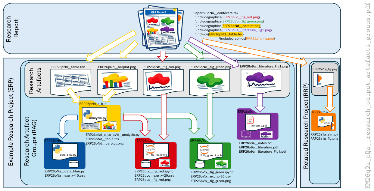
Figure 2.
Linking of research artefact groups (RAGs). (a) Illustration of RAG ERP26q3b linked to five predecessor RAGs, which were generated at different times. (b) Notebook excerpt showing a concept study of the illustration in panel (a). The filenames of the graphics included in the LATEX file of this article are listed below the graphics. The filename of the left-hand figure indicates that it has been derived from the notes depicted in the right-hand panel, which reference the respective RAG KM26q3a and the date 03.03.2026.
Figure 2.
Linking of research artefact groups (RAGs). (a) Illustration of RAG ERP26q3b linked to five predecessor RAGs, which were generated at different times. (b) Notebook excerpt showing a concept study of the illustration in panel (a). The filenames of the graphics included in the LATEX file of this article are listed below the graphics. The filename of the left-hand figure indicates that it has been derived from the notes depicted in the right-hand panel, which reference the respective RAG KM26q3a and the date 03.03.2026.
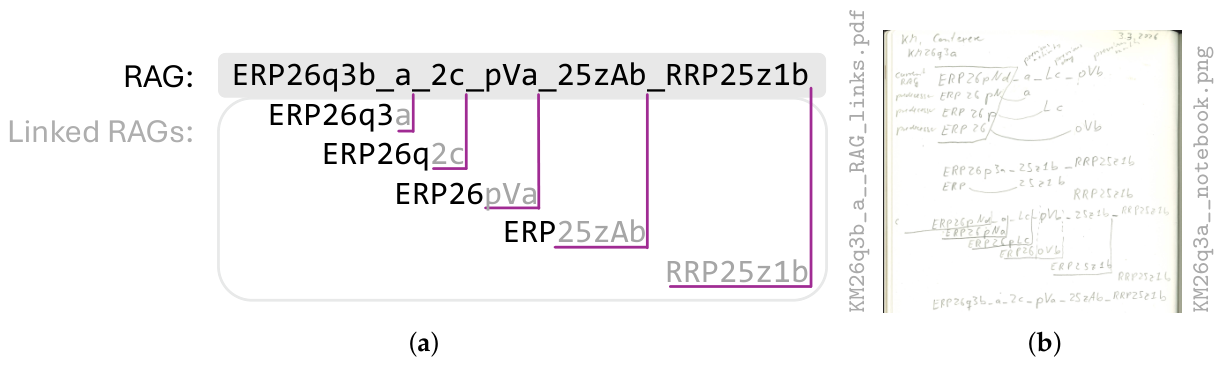
Figure 3.
Command line interface of the nxt command provided by the Python package contexere.
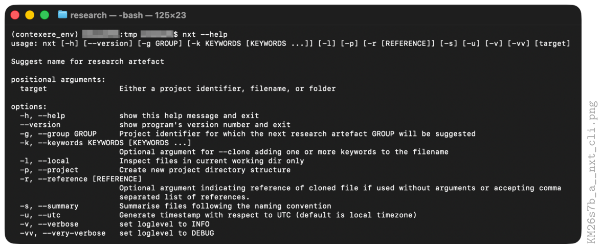
Figure 4.
Annotated screenshot of the command line dialogue generating a new project structure (a) and resulting project tree (b) with automatically generated first logbook entry (b, bottom). Arrows indicate the information flow from the dialogue to the generated project template. The vertical filename on the right-hand side indicates RAG KM26s6j_i_f linking the figure to project KM (short for Knowledge Management). The work on this figure started on May 2026 (26s6). It was the tenth KM artefact (j) generated on this day and was derived from research artefacts KM26s6i and KM26s6f. These RAGs reference the redacted screenshots.
Figure 4.
Annotated screenshot of the command line dialogue generating a new project structure (a) and resulting project tree (b) with automatically generated first logbook entry (b, bottom). Arrows indicate the information flow from the dialogue to the generated project template. The vertical filename on the right-hand side indicates RAG KM26s6j_i_f linking the figure to project KM (short for Knowledge Management). The work on this figure started on May 2026 (26s6). It was the tenth KM artefact (j) generated on this day and was derived from research artefacts KM26s6i and KM26s6f. These RAGs reference the redacted screenshots.
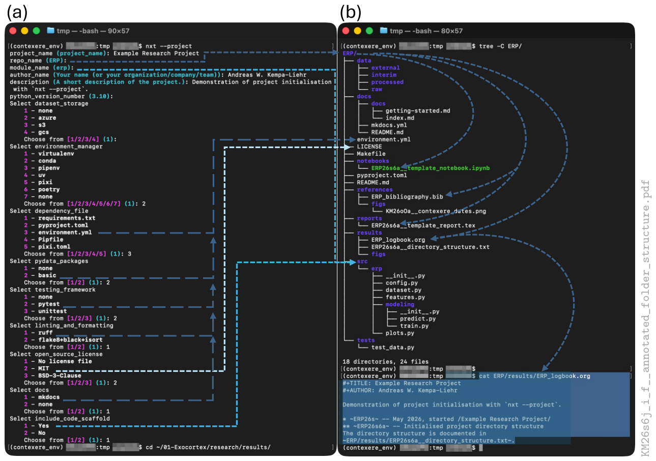
Figure 5.
Screenshot of the template Jupyter notebook. (a) Notebook ERP26s6a__template_notebook.ipynb generated by the command line dialogue in Figure 4 with option pydata_packages set to basic. (b) Alternative notebook configuration if option pydata_packages had been set to none. Note, that the respective ERQ project had been generated with nxt --project on 8 May 2026 (ERQ26s8a), two days after generating the ERP project (Figure 4). The filename references below the screenshots indicate that the respective files were created on 8 May 2026 (KM26s8) as part of the KM project.
Figure 5.
Screenshot of the template Jupyter notebook. (a) Notebook ERP26s6a__template_notebook.ipynb generated by the command line dialogue in Figure 4 with option pydata_packages set to basic. (b) Alternative notebook configuration if option pydata_packages had been set to none. Note, that the respective ERQ project had been generated with nxt --project on 8 May 2026 (ERQ26s8a), two days after generating the ERP project (Figure 4). The filename references below the screenshots indicate that the respective files were created on 8 May 2026 (KM26s8) as part of the KM project.
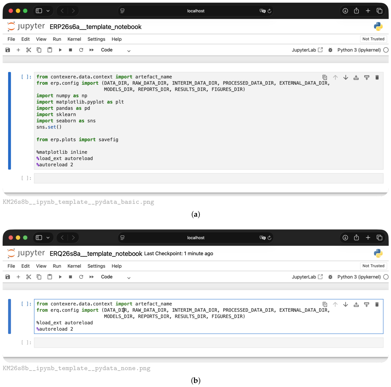
Figure 6.
Screenshot showing the initialisation of a local git repository capturing a project scaffold generated with nxt --project. In addition, the tagging of the first commit is demonstrated. Note, that the assigned tag ERP26s6a matches the respective logbook entry (lower bottom of Figure 4).
Figure 6.
Screenshot showing the initialisation of a local git repository capturing a project scaffold generated with nxt --project. In addition, the tagging of the first commit is demonstrated. Note, that the assigned tag ERP26s6a matches the respective logbook entry (lower bottom of Figure 4).
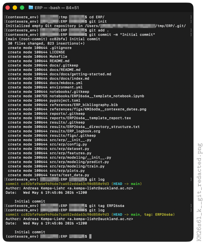
Figure 7.
Screenshot of command line dialogues using the project-specific Python environment generated with make create_environment. (a) Activation of the newly generated virtual environment ERP and importing the project-specific Python package erp. The project-specific Python package includes a config module that defines variables for the project’s relevant paths. (b) Building and serving of project documentation. (c) Web browser showing the interactive project documentation provided by a local web server.
Figure 7.
Screenshot of command line dialogues using the project-specific Python environment generated with make create_environment. (a) Activation of the newly generated virtual environment ERP and importing the project-specific Python package erp. The project-specific Python package includes a config module that defines variables for the project’s relevant paths. (b) Building and serving of project documentation. (c) Web browser showing the interactive project documentation provided by a local web server.
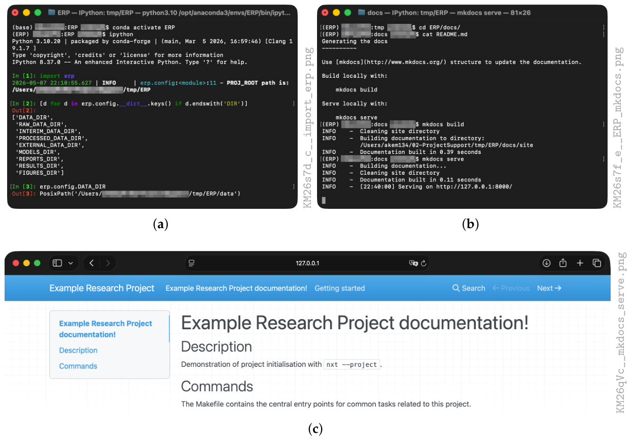
Figure 8.
Applications of the nxt command in the context of a newly generated project (cf. Figure 4). (a) In an empty directory, the nxt command returns the abbreviated date appended by the first step counter “a”. (b) At the root of a directory with existing RAG filenames, the next RAG of the latest project identifier is returned. (c) Overview of RAGs collected by traversing the folder hierarchy. (d) Cloning of an existing file advanced the RAG accordingly. (e) Cloned files are added automatically to the git repository.
Figure 8.
Applications of the nxt command in the context of a newly generated project (cf. Figure 4). (a) In an empty directory, the nxt command returns the abbreviated date appended by the first step counter “a”. (b) At the root of a directory with existing RAG filenames, the next RAG of the latest project identifier is returned. (c) Overview of RAGs collected by traversing the folder hierarchy. (d) Cloning of an existing file advanced the RAG accordingly. (e) Cloned files are added automatically to the git repository.
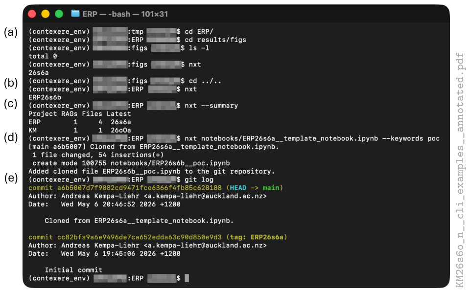
Figure 9.
Screenshots showing the automated naming and metadata annotation of a research artefact figure. (a) Example notebook ERP26s9b__poc.ipynb using function artefact_name() (Cell [2]) to retrieve the notebook name and the saving of a PDF figure in the project-specific results/figs folder (Cells [6] and [8]). (b) The metadata of the generated PDF document references the author, research project, and generating script.
Figure 9.
Screenshots showing the automated naming and metadata annotation of a research artefact figure. (a) Example notebook ERP26s9b__poc.ipynb using function artefact_name() (Cell [2]) to retrieve the notebook name and the saving of a PDF figure in the project-specific results/figs folder (Cells [6] and [8]). (b) The metadata of the generated PDF document references the author, research project, and generating script.
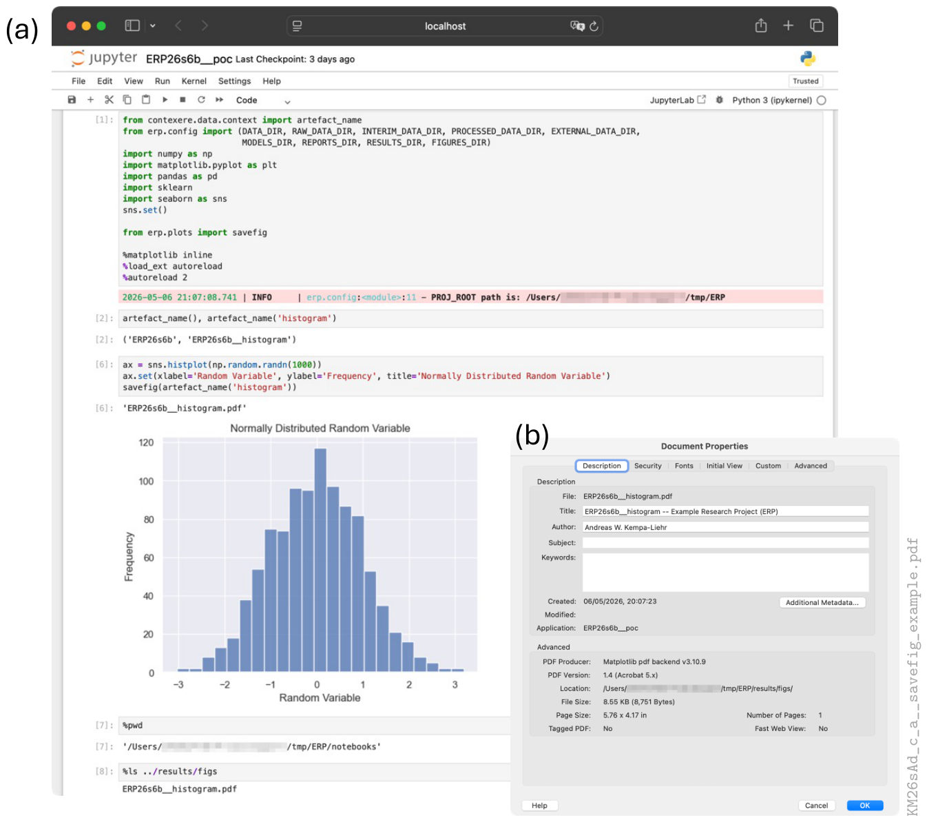
Figure 10.
Integrating research artefact figures into logbook or reports using markup languages. The examples given build on the hypothetical ERP project described in the previous sections. (a) Emacs screenshot of the extended ERP_logbook.org, which was introduced in its template version in Figure 4b. (b) Emacs screenshot of the LATEX document cloned and modified from ERP/reports/ERP26s6a_example_report.tex. (c) Screenshot of the PDF document created from the Org Mode document shown in panel (a). (d) Output of the \copyrightbox macro shown in panel (b).
Figure 10.
Integrating research artefact figures into logbook or reports using markup languages. The examples given build on the hypothetical ERP project described in the previous sections. (a) Emacs screenshot of the extended ERP_logbook.org, which was introduced in its template version in Figure 4b. (b) Emacs screenshot of the LATEX document cloned and modified from ERP/reports/ERP26s6a_example_report.tex. (c) Screenshot of the PDF document created from the Org Mode document shown in panel (a). (d) Output of the \copyrightbox macro shown in panel (b).
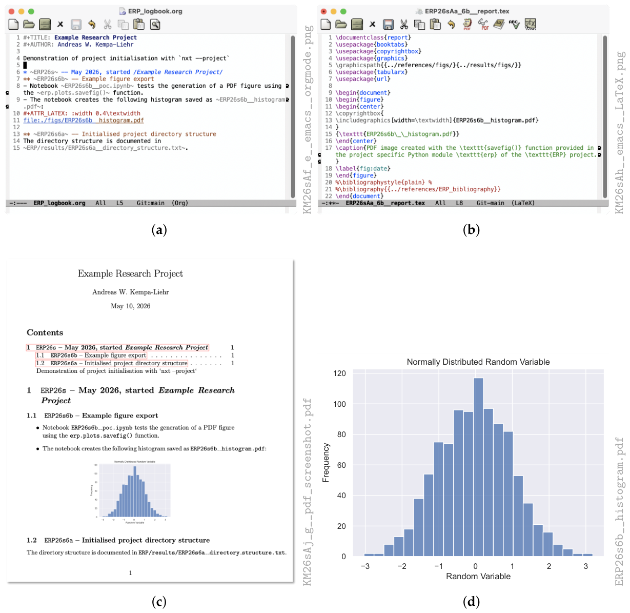
Figure 11.
Examples for documenting conversations with generative AI. (a) Redacted screenshot of Copilot conversion (left) and Microsoft Word document (right) with the exported conversation. (b) Redacted screenshot of Grok.com conversion (left) and Emacs (right) with the Org Mode export of the conversation.
Figure 11.
Examples for documenting conversations with generative AI. (a) Redacted screenshot of Copilot conversion (left) and Microsoft Word document (right) with the exported conversation. (b) Redacted screenshot of Grok.com conversion (left) and Emacs (right) with the Org Mode export of the conversation.
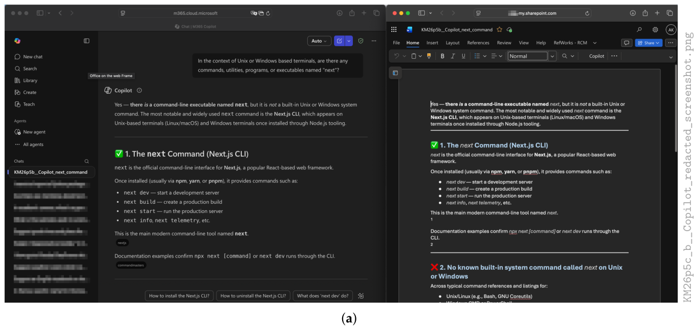
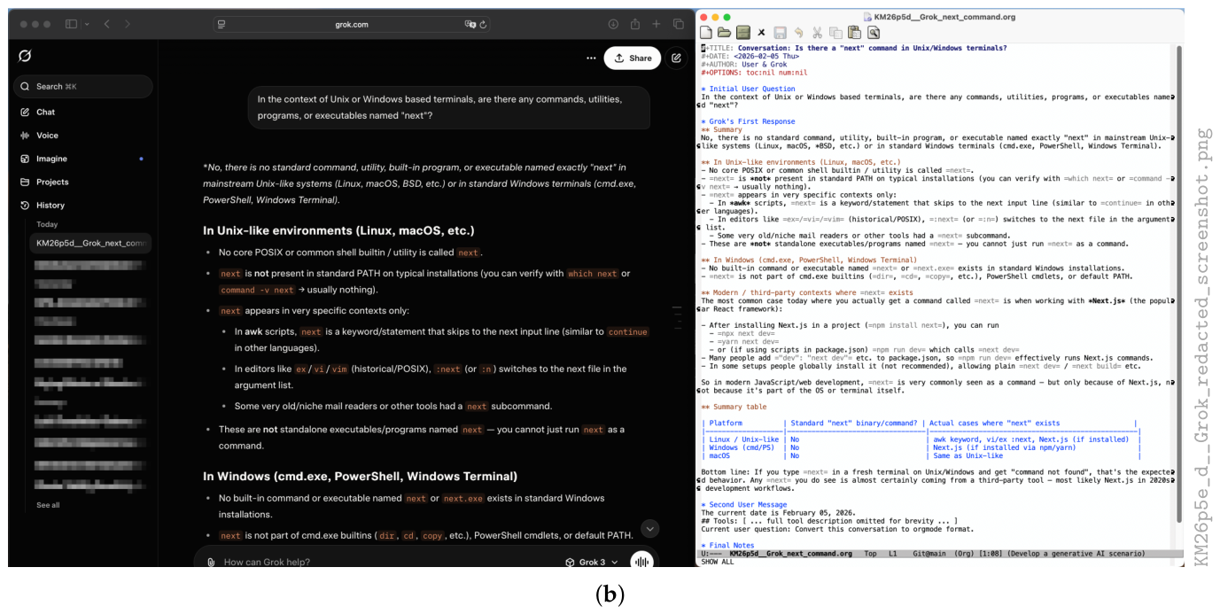
Figure 12.
Examples for documenting conversations with generative AI. (a) Screenshot of Gemini conversation (left) and Obsidian rendering the Markdown export of the conversation (right). (b) Screenshot of Claude.ai conversation with integrated PDF export.
Figure 12.
Examples for documenting conversations with generative AI. (a) Screenshot of Gemini conversation (left) and Obsidian rendering the Markdown export of the conversation (right). (b) Screenshot of Claude.ai conversation with integrated PDF export.
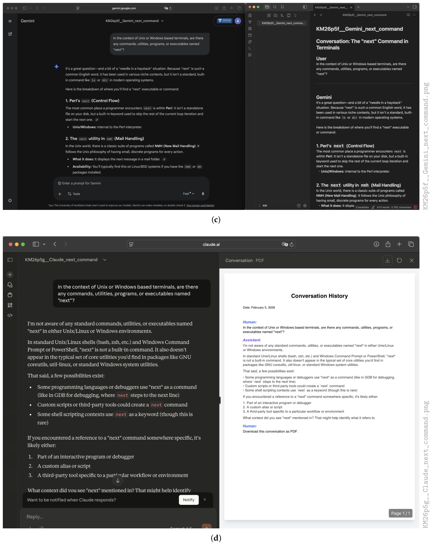

Table 1.
Month and day abbreviations for research artefact groups. The month-day abbreviation md is appended to the truncated two-digit year abbreviation yy [18], (p 12). E.g., the code 26q1 represents the date 2026-03-01 with just four key strokes.
Table 1.
Month and day abbreviations for research artefact groups. The month-day abbreviation md is appended to the truncated two-digit year abbreviation yy [18], (p 12). E.g., the code 26q1 represents the date 2026-03-01 with just four key strokes.
| Months | Days 1–10 | Days 11-20 | Days 21-31 | ||||
|---|---|---|---|---|---|---|---|
| m | Month | D | day | D | day | D | day |
| o | January | 1 | 1 | B | 11 | L | 21 |
| p | February | 2 | 2 | C | 12 | M | 22 |
| q | March | 3 | 3 | D | 13 | N | 23 |
| r | April | 4 | 4 | E | 14 | O | 24 |
| s | May | 5 | 5 | F | 15 | P | 25 |
| t | June | 6 | 6 | G | 16 | Q | 26 |
| u | July | 7 | 7 | H | 17 | R | 27 |
| v | August | 8 | 8 | I | 18 | S | 28 |
| w | September | 9 | 9 | J | 19 | T | 29 |
| x | October | A | 10 | K | 20 | U | 30 |
| y | November | V | 31 | ||||
| z | December | ||||||
Table 2.
Decoding the RAG identifiers of Figure 1 into Project identifier, date, and daily counter. Note that the alphabetical sorting of RAG identifiers creates a project-specific chronological list of RAGs.
Table 2.
Decoding the RAG identifiers of Figure 1 into Project identifier, date, and daily counter. Note that the alphabetical sorting of RAG identifiers creates a project-specific chronological list of RAGs.
| RAG | Project ID | Date | Daily Counter |
|---|---|---|---|
| ERP26oVb | ERP | 31.01.2026 | |
| ERP26p9a | ERP | 09.02.2026 | |
| ERP26pLc | ERP | 21.02.2026 | |
| ERP26pNa | ERP | 23.02.2026 | |
| ERP26pNd | ERP | 23.02.2026 | |
| RRP25z1a | RRP | 01.12.2025 |
Table 3.
Overview of generative AI experiments.
| Experiment | Service | URL | Export Format | Suffix | Figure |
|---|---|---|---|---|---|
| KM26p5b | Copilot | https://m365.cloud.microsoft/chat | Microsoft Word | .docx | Figure 11a |
| KM26p5c | Grok | https://grok.com | Org Mode | .org | Figure 11b |
| KM26p5e | Gemini | https://gemini.google.com | Markdown | .md | Figure 12a |
| KM26p5g | Claude | https://claude.ai | Portable Document Format | Figure 12b |
Disclaimer/Publisher’s Note: The statements, opinions and data contained in all publications are solely those of the individual author(s) and contributor(s) and not of MDPI and/or the editor(s). MDPI and/or the editor(s) disclaim responsibility for any injury to people or property resulting from any ideas, methods, instructions or products referred to in the content. |
© 2026 by the author. Licensee MDPI, Basel, Switzerland. This article is an open access article distributed under the terms and conditions of the Creative Commons Attribution (CC BY) license.
Copyright: This open access article is published under a Creative Commons CC BY 4.0 license, which permit the free download, distribution, and reuse, provided that the author and preprint are cited in any reuse.


