

Submitted:
14 May 2026
Posted:
14 May 2026
You are already at the latest version
Abstract
Algorithms based on gradient-boosted trees are known for predictive accuracy in tabular regression, while hybrid boosting designs adding non-tree terms remain underexplored. The present work introduces OPAL (Ordered Piecewise Additive Learner), a stagewise regression model combining hinge, categorical indicator, and regression-tree terms. Stage 1 of OPAL sequentially adds hinge and categorical indicator terms to squared loss residuals; Stage 2 fits regression-tree terms to the remaining residual structure. To increase expressiveness, OPAL augments the raw data with deterministic numeric transformations, including products, ratios, differences, signed square roots, log-modulus, and squared terms. OPAL can optionally fit a single tree before the two-stage model and train the main component on the resulting residuals. As regularization, inner cross-validation selects the prediction rule among the full predictor, the two-stage component alone, the optional single-tree component, the training-set mean, or a weighted blend. The rule is stored as fitted state, and the selected rule is reflected in a distilled additive prediction equation used for term-level summaries. Across 35 regression tasks, OPAL has the best average RMSE rank against XGBoost, LightGBM, and MARS: 1.857 versus 2.029, 2.429, and 3.686, respectively. A Friedman test rejects equality of ranks. Log-ratio paired tests do not separate OPAL from XGBoost but favor OPAL over LightGBM and MARS. The results support the strong predictive performance of the configured OPAL pipeline as a whole rather than any isolated algorithmic component; potential research directions, therefore, include further study of OPAL’s constituent parts. A unique aspect of OPAL is its partial additive transparency: hinge and categorical terms support effect-curve summaries when they have nonzero weight in the distilled prediction equation, although the full predictor may include generated pairwise features and tree terms involving the same raw variables.
Keywords:
linear basis functions
; boosted trees
; explainability
; tabular regression
1. Introduction
Algorithms based on gradient-boosted trees are a strong default for tabular regression [5,11,14]. A separate line of hybrid rule-based modeling has explored how tree-derived rule terms can be combined with simpler additive terms; RuleFit, for example, combines tree-derived rules with linear terms in a single regularized predictor [9]. One potential benefit of such hybrids is that they can pair the predictive strength of tree-based components with additional structure from other term families, such as additive or rule terms that are easier to inspect. OPAL (Ordered Piecewise Additive Learner) is motivated by a related question: can additive hinge and categorical terms be combined with residual regression-tree terms to retain competitive accuracy while exposing part of the fitted function through an inspectable structure?
Conceptually, OPAL seeks to improve post-fit transparency by separating Stage 1 additive terms on prepared columns from Stage 2 tree terms. Accordingly, the OPAL architecture defines two sequential stages of model fitting: Stage 1 adds prepared-feature hinge and categorical indicator terms to squared loss residuals, and Stage 2 adds regression-tree terms to the remaining residual structure. When enabled, a single-tree initializer is fit before these stages and its in-sample predictions are subtracted, so the two-stage model is trained on a residualized target. To guard against overfitting, OPAL then uses inner cross-validation to decide whether final predictions should be formed from the full hybrid predictor, the two-stage model alone, the optional single-tree initializer, the training-set mean, or a weighted blend of available predictions. The selected prediction scoring rule is stored with the fitted model and reused at prediction time.
The remainder of the paper evaluates whether this configured OPAL pipeline is both technically coherent and empirically competitive. First, it formalizes OPAL as a hybrid regression model whose Stage 1 terms include left and right hinge basis functions and categorical indicators, and whose Stage 2 terms add regression-tree corrections. Second, it describes the ordered residual-fitting procedure, including deterministic sample- and feature-aware budget shrinkage and the inner-CV prediction selector used for regularization. Finally, it evaluates OPAL on the 35-task CTR23 benchmark against XGBoost, LightGBM, and MARS, followed by a brief example of the interpretability afforded by the distilled additive term representation. The paper does not make broad interpretability claims for the full predictor; rather, it argues that OPAL’s Stage 1 additive component provides a more transparent, albeit partial, view of selected prepared-feature effects than traditional black-box tabular regression algorithms.
2. Related Work
OPAL sits at the intersection of additive spline and hinge models, rule-based hybrids, and modern tree ensembles. Generalized additive models (GAMs) [12,13,22] represent a response through sums of smooth feature functions, while multivariate adaptive regression splines (MARS) [8] builds adaptive spline regressions from piecewise-linear hinge basis functions. MARS therefore provides the hinge-basis lineage most directly connected to OPAL’s Stage 1 terms. RuleFit [9] combines tree-derived rules and linear terms in a single regularized predictor. OPAL differs from these approaches by using an ordered residual-fitting design: hinge and categorical indicator terms are fitted first, and regression-tree terms are then added to the residuals that remain.
GA2M models [16] and explainable boosting machines (EBMs) [18] extend the additive-model line by retaining inspectable main-effect functions while allowing selected pairwise interactions or boosted tree-shaped functions. Neural additive models (NAMs) [1] and GAMI-Net [23] replace some of the function-estimation machinery with neural subnetworks while preserving additive main effects and, in GAMI-Net, structured pairwise interactions. OPAL instead uses hinge and categorical terms in Stage 1, then uses regression-tree rules as a downstream residual term family.
The hinge and categorical terms retained by OPAL are auditable because each exposes its prepared feature, threshold or level, direction where applicable, and fitted weight. The position taken herein is a limited transparency claim rather than a claim of full-model interpretability, as generated pairwise columns can enter Stage 1, and the deployed predictor can also include regression-tree terms, an optional initial tree component, and an internally selected component blend.
3. The OPAL Framework
3.1. Feature Preparation and Deterministic Augmentation
OPAL first converts raw tabular inputs into a deterministic prepared matrix. Numeric predictors are coerced to numeric form and median-imputed. In the benchmark presented in a subsequent section, categorical predictors are converted to strings after replacing missing values with a reserved __MISSING__ token. If a training-split categorical column has more than max_cat_levels=1000 distinct levels, only the 999 most frequent training levels are retained and all other levels are mapped to __OTHER__; columns with at most 1000 levels keep all observed training levels. The mapped training column is then encoded with scikit-learn’s OrdinalEncoder using its fitted categories_ order. Evaluation levels not present after training-split mapping are assigned one code above the largest training code for that column. The numeric and categorical blocks are then merged into contiguous floating-point matrices. The implementation carries the categorical-column indices forward: Stage 1 treats those columns through equality indicators, and Stage 2 uses one-versus-level equality splits rather than ordered threshold splits on the ordinal codes.
The prepared matrix may be augmented with deterministic transformed numeric features; the enabled transform set is shown in Table 1. Only numeric columns participate in this construction. Remaining non-finite numeric values are mapped to zero, and each numeric column receives a deterministic continuous-target mutual information (MI) relevance score [4,15,19]. If MI scoring is unavailable, the implementation uses training variance as a fallback. For pairwise features, OPAL enumerates numeric-column pairs in increasing prepared-column order with , ranks pairs by the sum of their two relevance scores, and relies on the stable sort to preserve this enumeration order for ties. The configured pair budget is therefore a budget on retained numeric pairs, not on final generated columns. In the benchmark this pair budget is 30. Each retained pair is expanded in the fixed order product, ratio, difference when those transforms are enabled; the ratio and difference are one-directional, and , using the same orientation. Unary transforms are added in a separate pass: OPAL ranks individual numeric columns by their own relevance scores, retains columns for pair budget K, and appends the enabled signed square-root, signed logarithm of one plus absolute value, and square transforms. With the benchmark value , this unary pass considers seven numeric columns before the later variance and MI filters.
For numerical stability, generated columns are processed using training-split statistics before they enter the model. Product, difference, signed square-root, signed logarithm of one plus absolute value, and square columns are winsorized to the training 1st–99th percentiles. Ratio columns use the stabilized denominator and are then clipped to the same training percentile range.
After generation, transformed columns are standardized using training-set moments, clipped to , and stripped of near-constant columns. If generated columns remain, a final deterministic MI filter keeps columns whose generated-feature score is at least 10% of the maximum generated-feature score or belongs to the top half of generated columns. The surviving generated columns are appended to the prepared matrix. This is supervised, training-split feature preparation rather than a Stage 1 or Stage 2 fitted term family: the MI scores, retained generated columns, winsorization limits, and standardization moments are learned only inside the relevant training fold and then applied to that fold’s evaluation rows.
3.2. Prediction Function and Components
The stagewise main component of OPAL is an additive residual model over the prepared matrix. Before the final ridge calibration described below, it uses two high-level fitted term families, with categorical indicators included in the first stage:
Here indexes left and right hinge terms, indexes categorical indicator terms selected during Stage 1, and indexes regression-tree rules selected during Stage 2. The hinge basis uses prepared-feature index , threshold , and direction . The tree term maps an input row to its assigned leaf value, and is the corresponding ridge-scaled tree weight. All stagewise updates in the reported benchmark use squared loss on the standardized training target, so the negative gradients used for fitting are ordinary residuals. The weights in Equation (1) are the internal stagewise term weights before the final ridge calibration.
When the optional initial tree component is enabled, OPAL first standardizes the target, fits a single regression tree, and subtracts that tree’s predictions on the original training rows. The initializer uses the non-matrix fit path: for it trains on a seeded permutation containing every training row exactly once, while for it trains on a seeded with-replacement draw of size n. The fitted initializer is then evaluated on the original training and evaluation rows, and its original-training predictions are subtracted before fitting the stagewise main component in Equation (1). In the code this option is controlled by the pretrain_* configuration fields; the paper refers to it as the initial tree component or single-tree residual initializer.
After the stagewise main component has been fit, the canonical benchmark path applies a one-column ridge refit to calibrate the main-component prediction. Let denote the standardized target used by the main component: the standardized target itself when no initializer is used, and the residualized standardized target when the initializer is used. Let be the uncalibrated main-component prediction on training row i. With and , OPAL solves
using the fixed benchmark value . The calibrated main component is . This ridge refit does not introduce new basis functions and does not refit individual hinge, categorical, or tree terms; it only applies a global slope and intercept to the stagewise main-component prediction. Centered contribution curves for the main component can therefore be shown on the calibrated scale by multiplying the corresponding stagewise contributions by .
What is referred to here as the full component includes the calibrated main component plus the configured scaled initial-tree contribution, while the main component excludes that initial tree. The benchmark subtracts the unscaled initializer during residualization but adds back 97% of it in the full component. This is a fixed implementation choice intended to damp the initializer when it is recombined with the main residual model; it is not tuned inside the benchmark and is not presented as an optimal value. The current experiments do not include an ablation or sensitivity analysis over this constant, so the empirical results presented herein should be read as results for the configured OPAL system with this scale fixed. The inner-CV selector can still reject the full component in favor of the main component, the initializer alone, the training-set mean, or their simplex blend.
3.3. Stage 1: Hinge and Categorical Terms
For a prepared numerical feature indexed by j and threshold t, OPAL considers both hinge directions:
The candidate threshold grid for each prepared numerical feature is built once from the full training column before row subsampling is applied. Let denote the sorted unique finite values in that column and let denote the effective value of n_quantiles after the internal capacity adjustment in Section 3.6. If , all unique values are used as candidate thresholds. If , OPAL uses the linearly interpolated empirical percentiles of the unique-value vector at probabilities for , then removes duplicate threshold values. Categorical columns do not use hinge thresholds; they contribute equality-indicator candidates.
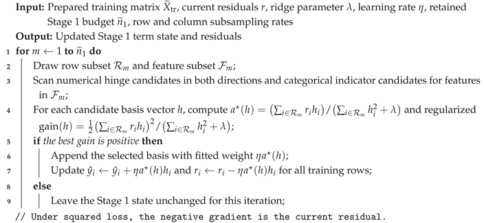
At Stage 1 iteration m, OPAL samples a row set without replacement using the tuned subsample value. With n training rows and subsampling rate s, the sampled size is when and all n rows otherwise. It also samples a candidate feature set using colsample_bytree; with p prepared features and column-sampling rate c, the sampled feature count is when and all p features otherwise. Candidate scoring scans only features in and computes the score over rows in . Given current residual vector r, ridge parameter , and a candidate basis vector h, the unshrunk one-coordinate ridge coefficient and the associated regularized gain score are
This score is the one-coordinate ridge objective improvement used for candidate selection, not the unpenalized squared-loss reduction after shrinkage. The selected term receives the post-shrinkage weight , where is the global learning rate for the stagewise update, and its prediction contribution is then applied to all training rows when residuals are updated. For categorical predictors, the candidate basis is ; the same coefficient and gain formulas apply with . Stage 1 repeats this greedy residual-fitting step for the retained main-term budget, adding the best hinge or categorical indicator candidate at each successful iteration. If the best gain is non-positive, the implementation advances without adding a term. Algorithm 1 summarizes the Stage 1 update.
| Algorithm 1:Stage 1: hinge and categorical residual fitting |
 |
3.4. Stage 2: Regression-Tree Rule Terms
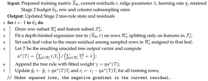
After Stage 1, OPAL fits regression-tree rule terms to the remaining residuals. At tree iteration t, OPAL draws a row subset and a tree feature subset using the same sample-size rules as Stage 1. The tree is fit on and is allowed to split only on features in . In the benchmarked histogram tree path, numeric prepared features reuse the same global quantile grids described above, with thresholds per feature before duplicate removal; at each node OPAL evaluates the available grid thresholds and accepts only splits satisfying the minimum-leaf constraint on the sampled rows in that node. Categorical prepared features use equality splits of the form versus , so their ordinal codes are not treated as ordered quantities inside Stage 2. Each tree greedily chooses splits that reduce within-node residual variance, subject to the configured depth and minimum-leaf constraints. Leaf values are the mean residuals among sampled rows in that reach the leaf, not the mean over all training rows assigned by the final split structure. Once a tree output vector T is grown, OPAL applies a scalar ridge rescaling computed on the sampled rows,
then applies the scaled tree to all training rows and updates the residuals. The tree stage stops growing individual trees at the configured maximum depth, when too few samples remain in a node, or when no valid split is available. Algorithm 2 summarizes the Stage 2 update.
| Algorithm 2:Stage 2: regression-tree residual fitting |
 |
3.5. Internal Prediction Regularization
As a final regularization layer, OPAL uses inner cross-validation to choose among the full model, the initial tree component, the main component, the target-mean baseline, or a simplex-weighted blend of these predictions; the selected rule is stored as fitted model state. For each candidate configuration, OPAL fits the model on each inner-training fold, predicts the available components on the corresponding inner-validation fold, and stacks those out-of-fold component predictions against the inner-validation targets. Candidate components and the simplex stack are scored by RMSE on the pooled out-of-fold validation rows. The component selector or stack is learned and scored on the same pooled out-of-fold prediction matrix, so this value is a model-selection criterion for OPAL rather than an unbiased estimate of the selected rule’s generalization error. The selected rule is carried with the selected hyperparameter candidate and reused when the model is refit on the full outer-training split. It is therefore internal model selection/regularization rather than post-hoc tuning on the outer test data.
For auditing, OPAL materializes a full distilled additive prediction equation after the prediction rule has been selected. This equation applies the stored rule’s component weights to the fitted intercept, initializer, Stage 1 terms, and Stage 2 terms, so every displayed term contribution respects the deployed prediction rule. If the selected rule is the training-set mean or the initializer alone, the Stage 1 and Stage 2 terms receive zero weight in the distilled equation; if the selected rule is a simplex blend, each term is scaled by the corresponding component weight. Thus effect curves are summaries of terms that survive in the rule-weighted distilled equation, not explanations of components that the selector has excluded.
When the stack is selected, the code fits nonnegative component weights that sum to one and uses no free intercept, so the stacked prediction remains a convex combination of the available component predictions. Otherwise, the stored rule selects a single component by name. The target-mean component is included as a conservative baseline option, and the main component specifically denotes the Stage 1 plus Stage 2 fit after any residual initialization.
3.6. Budget Shrinkage and Stopping
OPAL applies deterministic capacity regularization to the provisional Stage 1 and Stage 2 iteration budgets. The rule is GCV-inspired but is not stated here as a claim of strict GCV optimality. For a provisional stage budget , training size n, prepared feature count p, prune quantile , and prune scale , define and and set
The retained budget is
The feature count p is the number of columns in the prepared matrix after deterministic augmentation, near-constant generated-column removal, and the generated-feature MI filter. In the benchmark code, the stage1_prune_* controls apply to the Stage 1 hinge/indicator budget n_main_estimators, while the stage2_prune_* controls apply to the Stage 2 tree budget n_interact_estimators. The benchmarked configuration leaves the enhanced early-stopping mode disabled, so reported fits use fixed retained budgets after deterministic shrinkage.
The OPAL algorithm also applies a fixed small-sample capacity prior after the above budget shrinkage. This prior is not tuned by Optuna. With training size n, prepared feature count p, effective rows-per-feature ratio , reference size 2000, and reference rows-per-feature value 10, define
For the effective quantile count , OPAL sets
with a final lower bound of one when n is very small. For the minimum leaf size , it computes and raises the leaf size to . If , the ridge parameter is moved toward 10 by replacing it with ; otherwise it is unchanged. Finally, the retained Stage 2 budget is replaced by . The Stage 1 budget is not further reduced by this prior.
3.7. Workflow Summary
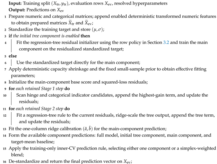
OPAL training proceeds in a fixed order. The estimator first prepares the numeric and categorical predictors and appends any enabled deterministic transformed features. If the initial tree component is enabled, a single tree is fit to the standardized target and the main component is trained on the residualized standardized target. The retained Stage 1 and Stage 2 budgets are then set by deterministic capacity shrinkage and the fixed small-sample prior. Stage 1 adds hinge and categorical indicator terms to residuals; Stage 2 adds regression-tree rule terms to the remaining residuals. The fitted main-component prediction is then ridge-calibrated with a single slope and intercept. Finally, OPAL forms the available component predictions, applies the stored inner-CV prediction rule, and de-standardizes the selected or blended prediction. Algorithm 3 lists the sequential workflow, and Figure 1 summarizes the same flow visually.
| Algorithm 3:Sequential OPAL training and prediction workflow |
 |
4. Experimental Results
4.1. Benchmark Setup
The benchmark uses the 35 OpenML-CTR23 tabular regression tasks of Fischer et al. [7], accessed through OpenML [21] and the task-provided outer splits. Appendix Table A1 lists the data-set-level RMSE results. The present empirical comparison includes exactly four models: OPAL, XGBoost, LightGBM, and MARS. Five tasks expose 10 repeats, 10 folds, and one sample, giving 100 outer splits per task. The remaining 30 tasks expose one repeat, 10 fold indices, and one sample, giving 10 outer splits per task. The size-regime labels in Figure 2 are the nominal CTR23 labels; even tasks in the large-data/holdout regime are evaluated here using the OpenML task-provided split indices rather than a newly generated 33% holdout split. Figure 2 summarises the suite by OpenML row count and raw predictor count.
Within each outer training split, the benchmark driver uses deterministic inner tuning splits chosen by sample size: 10-fold inner cross-validation when , 3-fold inner cross-validation when , and a 33% holdout when . Each model is tuned independently on each outer training split by an Optuna RandomSampler seeded from the split seed, with n_trials and n_jobs in the canonical benchmark invocation. XGBoost, LightGBM, and MARS minimize the unweighted mean RMSE across the deterministic inner splits. OPAL minimizes the pooled out-of-fold RMSE of its internally selected component rule for the candidate configuration, because the candidate includes the inner-CV component selector described in Section 3.5. These objectives are therefore not algebraically identical; the difference is part of OPAL’s internal model-selection procedure, and the OPAL inner score is not used as a benchmark performance estimate. The comparative results use only the common outer-split RMSE values. After optimization, the best completed trial is refit on the full outer training split and evaluated once on the corresponding outer test rows. For each data set and model, the reported data-set-level RMSE is the unweighted arithmetic mean of the resulting outer-split RMSE values; ranks and cross-data-set statistical tests use these data-set-level means rather than pooled out-of-fold RMSE or test-size-weighted RMSE. Table 2 lists the nine OPAL hyperparameters tuned in the benchmark.
For OPAL, only the nine user-exposed tuning parameters in Table 2 are optimized. The displayed n_main and n_interact ranges are sampled provisional budgets after the fixed benchmark estimator-scale factor is applied; deterministic capacity shrinkage is applied after sampling. The initial tree component, its 0.97 full-component scale, the one-column ridge-refit penalty , transformed-feature construction, and the transformed-feature pair budget are fixed. The enabled transforms are product, ratio, sqrt, log, square, and diff; as described in Section 3.1, means at most 30 ranked numeric pairs before expansion, with seven unary columns considered before filtering. The final number of appended generated columns can be smaller after near-constant removal and the generated-feature MI filter. The prune quantiles are both 1.0, and the prune scale parameters are both 12.0. The sampled raw Stage 1 and Stage 2 estimator budgets are first shrunk deterministically by the rule in Section 3.6; the canonical implementation path then applies the fixed small-sample capacity prior defined in the same section, which can further change the effective n_quantiles, min_leaf, , and Stage 2 budget. The optional internal early-stopping path is disabled. XGBoost and LightGBM are likewise fit without validation-set early stopping, and MARS has no learner-specific early-stop mechanism in the harness. Table 3 gives the corresponding baseline search spaces.
Preprocessing is deterministic within each split, as described in Section 3.1. For XGBoost and LightGBM, numeric columns are median imputed and categorical columns use the same missing-token and 1000-level rare-category map before one-hot encoding with unseen levels ignored. MARS receives a dense numeric and ordinal representation built from the same split-local imputation and rare-level handling as OPAL. The MARS baseline uses the in-repository py-earth implementation [20]. In addition to the tuned knobs in Table 3, the wrapper enables use_fast=True when that constructor argument is available and, unless overridden, sets fast_K=25 and fast_h=1; no benchmark override changes those fast-mode settings.
Implementation-wise, OPAL is exposed through a scikit-learn compatible Python estimator. Aside from that wrapper and benchmark orchestration, the core fit/predict path and much of the term-generation logic are implemented in Mojo, a programming language developed by Modular for high-performance systems and numerical code [17]. The reported run uses base seed 1, jobs=4, and optuna_jobs=1. For OPAL, the split seed is the stable hash of the base seed, task ID, dataset ID, OPAL’s split-seed stream label, the outer split index, and the string split. For XGBoost, LightGBM, and MARS, the split seed is the stable hash of the base seed, task ID, dataset ID, model name, outer split index, and split. Inner split seeds are stable hashes of the split seed and inner, and Optuna sampler seeds are stable hashes of the split seed and optuna. OPAL also uses a fixed additional stable-seed stream for the initial tree component.
The timing columns report wall-clock measurements from this local invocation, not portable speed claims. The run was executed on an Apple M3 Max system with 16 logical cores and 128 GiB RAM under macOS arm64. The Python environment used Python 3.9.6, NumPy 2.0.2, pandas 2.3.3, SciPy 1.13.1, scikit-learn 1.6.1, Optuna 4.8.0, XGBoost 2.1.4, LightGBM 4.6.0, and OpenML 0.15.1. Because OPAL uses a Mojo core while the baselines rely on external library implementations, the reported tuning times should be interpreted as run-specific implementation evidence rather than portable algorithmic speed comparisons.
Performance is measured by RMSE, and ranks are assigned within each data set so that rank 1 denotes the lowest RMSE. All four models produced results on all 35 CTR23 tasks, so the aggregate summaries and complete-case significance tests use the same 35 data sets.
4.2. Statistical Analysis
Average RMSE rank is the primary omnibus summary. We use a Friedman omnibus test over the four current models and then a Nemenyi critical-difference view in the standard multi-data-set comparison tradition [6,10]. Because mean-rank post-hoc procedures have known limitations [2,3], and because the OPAL–boosting gaps are small, we also report paired Wilcoxon signed-rank tests on per-data-set log RMSE ratios, . This normalized test is invariant to target-scale changes across data sets. The Wilcoxon values reported in Table 5 are two-sided unadjusted p values; Holm-adjusted values are reported in the prose where they affect interpretation.
4.3. Aggregate Accuracy Results
Table 4 summarises the aggregate results. OPAL has the best average RMSE rank among the four evaluated methods: 1.8571 for OPAL, 2.0286 for XGBoost, 2.4286 for LightGBM, and 3.6857 for MARS. For each data set, the RMSE ratio divides a model’s RMSE by the lowest RMSE achieved by any of the four evaluated models on that data set; the table reports the geometric mean of those ratios across data sets. OPAL has the lowest geometric mean RMSE ratio, 1.0650, and the most first-place finishes, 17 of 35 tasks. XGBoost remains close, with the most top-two finishes (26 versus 24 for OPAL). In this run, MARS has the lowest median tuning time because its search space is lightweight, but it has the weakest average rank. OPAL’s recorded median tuning time is lower than the two boosted-tree baselines (440.9 s versus 595.8 s for XGBoost and 612.5 s for LightGBM), with the environment-specific caveat described above.
The OPAL/XGBoost comparison is close: OPAL has lower RMSE on 19 of 35 tasks, while XGBoost has lower RMSE on 16 of 35 tasks. The two-sided paired Wilcoxon test on log RMSE ratios gives , so the two methods are not statistically distinguishable in this benchmark. OPAL has lower RMSE than LightGBM on 23 of 35 tasks; the log-ratio Wilcoxon value is and remains below 0.05 after Holm adjustment (), although the Nemenyi rank comparison below does not separate the two methods. OPAL has lower RMSE than MARS on 33 of 35 tasks, with a much smaller log-ratio Wilcoxon value ().
Average rank compresses meaningful variation in per-task placement. Figure 3 reports the full within-task rank distribution. OPAL and XGBoost occupy most of the upper ranks, LightGBM remains competitive but more often falls behind the top pair, and MARS is concentrated in fourth place.
The four-model Friedman test rejects equality of ranks (, ), and the Nemenyi critical distance is 0.793 at . OPAL and XGBoost differ by about 0.171 average-rank units and are not significantly different. OPAL and LightGBM differ by about 0.571 average-rank units, also below the critical distance, while OPAL and MARS differ by about 1.829 average-rank units, exceeding the critical distance. OPAL is effectively tied with XGBoost, has a scale-normalized paired advantage over LightGBM, and is stronger than the configured MARS baseline.
4.4. Stage 1 Interpretability Example
Figure 4 illustrates the narrow interpretability claim supported by OPAL’s term representation.
The image depicted in Figure 4 was generated from split 9 of OPAL’s fit on the cps88wages data set, where the stored prediction rule selected the full component and therefore gives the main Stage 1 terms nonzero weight in the distilled equation. Education was the top original Stage 1 hinge feature for this split, with 39 retained raw-feature hinge terms and thresholds at 13, 14, and 15 years of education. The curve therefore sweeps education across its observed range and uses only original-feature Stage 1 education terms; generated pairwise features, the initial tree component, and Stage 2 tree-rule corrections are excluded. The vertical axis is the centered Stage 1 contribution. Although this is not a full explanation of every prediction, it provides an auditable raw-feature slice that ordinary boosted-tree ensembles do not expose natively.
5. Conclusions
The present work establishes OPAL as a competitive two-stage hinge-and-tree learner for tabular regression. Deterministic preprocessing and optional transformed-feature construction prepare the design matrix; Stage 1 fits hinge and categorical indicator terms to residuals; Stage 2 fits regression-tree rules to the remaining residual structure. The current implementation also includes an optional initial tree component and an inner-CV prediction selector that chooses among model components or a simplex-weighted blend as fitted model state.
On the present 35-task CTR23 benchmark, OPAL attains the lowest average RMSE rank among OPAL, XGBoost, LightGBM, and MARS. The margin over XGBoost is small and not statistically significant. OPAL does not perform substantively better than LightGBM, as evidenced by the Nemenyi rank comparison, but the paired log-ratio Wilcoxon test favors OPAL on normalized RMSE differences. OPAL also improves over MARS under both views, but that conclusion is conditional on the MARS tuning range, dense numeric/ordinal representation, and fixed py-earth fast-mode settings used here [20]. The comparison should also not be read as a component ablation of OPAL; sensitivity to fixed implementation choices such as the 0.97 initializer scale remains a separate question that should be addressed through further research. The hinge terms remain directly auditable in the rule-weighted distilled equation, but the main contribution of this work is evidence for the configured OPAL pipeline rather than a broad claim about full-model interpretability. Overall, the results position OPAL as a strong alternative that sits between fully interpretable models and high-performance blackbox models, as it offers competitive performance with additional options for explainability using the Stage 1 main effect terms.
Appendix A. Full Benchmark Results

Table A1.
Full benchmark RMSE results using row-wise scientific notation. Each model cell reports a three-decimal mantissa with the within-row RMSE rank in parentheses; multiply each row by the right-hand scale. Rows are alphabetical by data set, and lower RMSE is better.
Table A1.
Full benchmark RMSE results using row-wise scientific notation. Each model cell reports a three-decimal mantissa with the within-row RMSE rank in parentheses; multiply each row by the right-hand scale. Rows are alphabetical by data set, and lower RMSE is better.
| Dataset | OPAL | XGBoost | LightGBM | MARS | Scale | |
|---|---|---|---|---|---|---|
| abalone | 2.061 (1) | 2.129 (4) | 2.122 (2) | 2.124 (3) | ||
| airfoil_self_noise | 1.313 (2) | 1.283 (1) | 1.510 (3) | 4.076 (4) | ||
| auction_verification | 0.835 (3) | 0.426 (2) | 0.374 (1) | 5.928 (4) | ||
| brazilian_houses | 3.061 (1) | 4.188 (3) | 8.266 (4) | 3.155 (2) | ||
| california_housing | 4.336 (1) | 4.526 (3) | 4.425 (2) | 6.376 (4) | ||
| cars | 2.200 (3) | 2.127 (1) | 2.129 (2) | 2.473 (4) | ||
| concrete_compressive_strength | 3.940 (2) | 3.811 (1) | 3.970 (3) | 6.289 (4) | ||
| cps88wages | 3.802 (2) | 3.802 (3) | 3.801 (1) | 3.811 (4) | ||
| cpu_activity | 2.057 (1) | 2.151 (2) | 2.225 (3) | 2.737 (4) | ||
| diamonds | 0.510 (1) | 0.534 (3) | 0.525 (2) | 1.874 (4) | ||
| energy_efficiency | 5.140 (3) | 2.951 (1) | 4.124 (2) | 5.393 (4) | ||
| fifa | 0.890 (1) | 0.896 (2) | 0.901 (3) | 1.050 (4) | ||
| forest_fires | 4.662 (4) | 4.581 (1) | 4.589 (2) | 4.646 (3) | ||
| fps_benchmark | 0.061 (1) | 0.061 (2) | 0.085 (3) | 4.508 (4) | ||
| geographical_origin_of_music | 1.540 (3) | 1.528 (2) | 1.516 (1) | 1.655 (4) | ||
| grid_stability | 0.594 (1) | 0.770 (2) | 1.418 (3) | 1.579 (4) | ||
| health_insurance | 1.443 (3) | 1.441 (2) | 1.440 (1) | 1.469 (4) | ||
| kin8nm | 0.881 (1) | 1.123 (2) | 1.434 (3) | 1.752 (4) | ||
| kings_county | 1.280 (3) | 1.131 (2) | 1.125 (1) | 1.972 (4) | ||
| miami_housing | 0.819 (3) | 0.814 (2) | 0.804 (1) | 1.285 (4) | ||
| Moneyball | 2.146 (2) | 2.230 (4) | 2.187 (3) | 2.126 (1) | ||
| naval_propulsion_plant | 0.530 (1) | 0.940 (3) | 8.182 (4) | 0.561 (2) | ||
| physiochemical_protein | 3.149 (1) | 3.335 (2) | 3.394 (3) | 4.968 (4) | ||
| pumadyn32nh | 2.122 (1) | 2.192 (2) | 2.922 (3) | 3.295 (4) | ||
| QSAR_fish_toxicity | 8.780 (2) | 8.650 (1) | 8.816 (3) | 9.302 (4) | ||
| red_wine | 5.539 (1) | 5.546 (2) | 5.738 (3) | 6.401 (4) | ||
| sarcos | 1.998 (1) | 2.193 (2) | 2.226 (3) | 5.140 (4) | ||
| socmob | 1.915 (3) | 1.195 (1) | 1.220 (2) | 2.430 (4) | ||
| solar_flare | 7.621 (1) | 7.632 (2) | 7.650 (3) | 7.886 (4) | ||
| space_ga | 0.959 (1) | 1.075 (3) | 1.117 (4) | 1.046 (2) | ||
| student_performance_por | 2.716 (3) | 2.671 (1) | 2.675 (2) | 2.755 (4) | ||
| superconductivity | 0.907 (3) | 0.902 (2) | 0.897 (1) | 1.912 (4) | ||
| video_transcoding | 0.083 (2) | 0.080 (1) | 0.103 (3) | 1.257 (4) | ||
| wave_energy | 0.310 (1) | 0.684 (3) | 0.576 (2) | 2.259 (4) | ||
| white_wine | 5.783 (2) | 5.743 (1) | 6.026 (3) | 7.256 (4) | ||
References
- Agarwal, R.; Melnick, L.; Frosst, N.; Zhang, X.; Lengerich, B.; Caruana, R.; Hinton, G. E. Neural additive models: Interpretable machine learning with neural nets. Adv. Neural Inf. Process. Syst. 2021, 34. [Google Scholar]
- Benavoli, A.; Corani, G.; Mangili, F. Should we really use post-hoc tests based on mean-ranks? J. Mach. Learn. Res. 2016, 17(5), 1–10. [Google Scholar]
- Benavoli, A.; Corani, G.; Demšar, J.; Zaffalon, M. Time for a change: A tutorial for comparing multiple classifiers through Bayesian analysis. J. Mach. Learn. Res. 2017, 18(77), 1–36. [Google Scholar]
- Brown, G.; Pocock, A.; Zhao, M.-J.; Luján, M. Conditional likelihood maximisation: A unifying framework for information theoretic feature selection. J. Mach. Learn. Res. 2012, 13, 27–66. [Google Scholar]
- Chen, T.; Guestrin, C. XGBoost: A scalable tree boosting system. In Proceedings of the 22nd ACM SIGKDD International Conference on Knowledge Discovery and Data Mining, 2016; pp. 785–794. [Google Scholar]
- Demšar, J. Statistical comparisons of classifiers over multiple data sets. J. Mach. Learn. Res. 2006, 7, 1–30. [Google Scholar]
- Fischer, S. F.; Feurer, M.; Bischl, B. OpenML-CTR23 – A curated tabular regression benchmarking suite. AutoML Conference 2023 (Workshop), 2023. [Google Scholar]
- Friedman, J. H. Multivariate adaptive regression splines. Ann. Stat. 1991, 19(1), 1–67. [Google Scholar] [CrossRef]
- Friedman, J. H.; Popescu, B. E. Predictive learning via rule ensembles. Ann. Appl. Stat. 2008, 2(3), 916–954. [Google Scholar] [CrossRef]
- García, S.; Herrera, F. An extension on “statistical comparisons of classifiers over multiple data sets” for all pairwise comparisons. J. Mach. Learn. Res. 2008, 9, 2677–2694. [Google Scholar]
- Grinsztajn, L.; Oyallon, E.; Varoquaux, G. Why do tree-based models still outperform deep learning on tabular data? Adv. Neural Inf. Process. Syst. 2022, 35, 507–520. [Google Scholar]
- Hastie, T.; Tibshirani, R. Generalized additive models. Stat. Sci. 1986, 1(3), 297–318. [Google Scholar] [CrossRef]
- Hastie, T.; Tibshirani, R. Generalized Additive Models; Chapman and Hall, 1990. [Google Scholar]
- Ke, G.; Meng, Q.; Finley, T.; Wang, T.; Chen, W.; Ma, W.; Ye, Q.; Liu, T.-Y. LightGBM: A highly efficient gradient boosting decision tree. Adv. Neural Inf. Process. Syst. 2017, 30. [Google Scholar]
- Kraskov, A.; Stögbauer, H.; Grassberger, P. Estimating mutual information. Phys. Rev. E 2004, 69(6), 066138. [Google Scholar] [CrossRef] [PubMed]
- Lou, Y.; Caruana, R.; Gehrke, J.; Hooker, G. Accurate intelligible models with pairwise interactions. In Proceedings of the 19th ACM SIGKDD International Conference on Knowledge Discovery and Data Mining, 2013; pp. 623–631. [Google Scholar]
- Modular. Mojo Manual (version 1.0.0b1). 2026. Available online: https://docs.modular.com/mojo/manual/ (accessed on 14 May 2026).
- Nori, H.; Caruana, R.; Bu, Z.; Shen, J. H.; Kulkarni, J. Accuracy, interpretability, and differential privacy via explainable boosting. Proc. 38th Int. Conf. Mach. Learn. 2021, PMLR 139, 8227–8237. [Google Scholar]
- Peng, H.; Long, F.; Ding, C. Feature selection based on mutual information: criteria of max-dependency, max-relevance, and min-redundancy. IEEE Trans. Pattern Anal. Mach. Intell. 2005, 27(8), 1226–1238. [Google Scholar] [CrossRef] [PubMed]
- Rudy, J. sklearn-contrib-py-earth 0.1.0: A Python implementation of Jerome Friedman’s Multivariate Adaptive Regression Splines. Python Package Index. 2017. Available online: https://pypi.org/project/sklearn-contrib-py-earth/ (accessed on 14 May 2026).
- Vanschoren, J.; van Rijn, J. N.; Bischl, B.; Torgo, L. OpenML: Networked science in machine learning. SIGKDD Explor. 2013, 15(2), 49–60. [Google Scholar] [CrossRef]
- Wood, S. N. Generalized Additive Models: An Introduction with R, 2nd ed.; CRC Press, 2017. [Google Scholar]
- Yang, Z.; Zhang, A.; Sudjianto, A. GAMI-Net: An explainable neural network based on generalized additive models with structured interactions. Pattern Recognit. 2021, 120, 108192. [Google Scholar] [CrossRef]
Figure 1.
OPAL workflow. Preparation and deterministic feature augmentation precede the fitted model. The fitted main component has two stages: Stage 1 fits hinge and categorical indicator terms, and Stage 2 fits regression-tree rule terms. The optional initial tree component, deterministic budget shrinkage and small-sample prior, one-column ridge calibration, and inner-CV prediction rule are regularization and model-state mechanisms rather than additional fitted stages.
Figure 1.
OPAL workflow. Preparation and deterministic feature augmentation precede the fitted model. The fitted main component has two stages: Stage 1 fits hinge and categorical indicator terms, and Stage 2 fits regression-tree rule terms. The optional initial tree component, deterministic budget shrinkage and small-sample prior, one-column ridge calibration, and inner-CV prediction rule are regularization and model-state mechanisms rather than additional fitted stages.
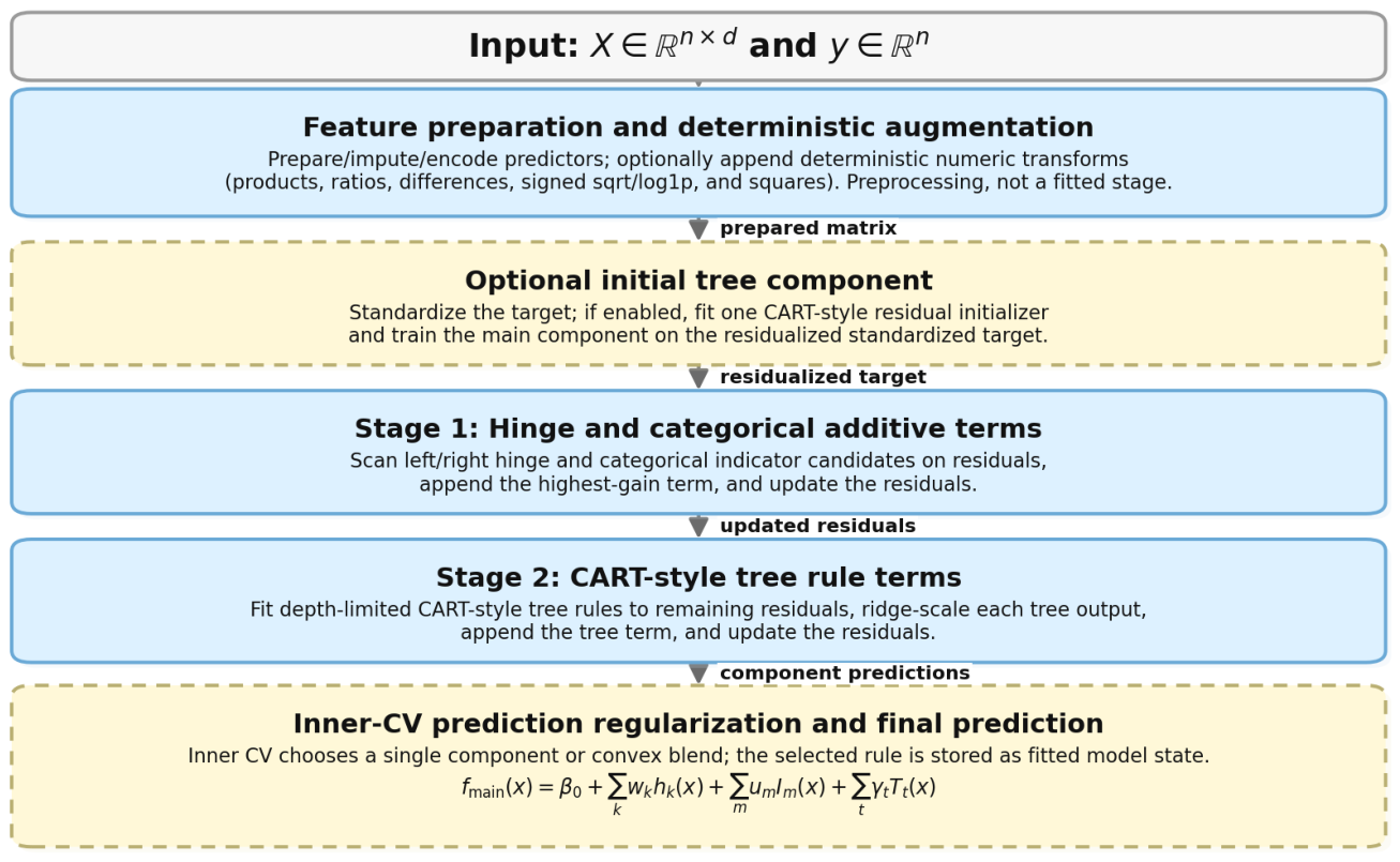
Figure 2.
Benchmark composition by data-set size. Each point is one CTR23 task. The horizontal axis reports the OpenML row count and the vertical axis reports the corresponding raw predictor count after excluding the target, ignored fields, and row identifiers; both axes are shown on log scales. Marker shape indicates the nominal CTR23 outer resampling regime, and the dashed vertical lines at 1000 and 10000 rows mark the thresholds used for those nominal regime labels; the actual OpenML split dimensions used in the reported run are described in the benchmark setup.
Figure 2.
Benchmark composition by data-set size. Each point is one CTR23 task. The horizontal axis reports the OpenML row count and the vertical axis reports the corresponding raw predictor count after excluding the target, ignored fields, and row identifiers; both axes are shown on log scales. Marker shape indicates the nominal CTR23 outer resampling regime, and the dashed vertical lines at 1000 and 10000 rows mark the thresholds used for those nominal regime labels; the actual OpenML split dimensions used in the reported run are described in the benchmark setup.
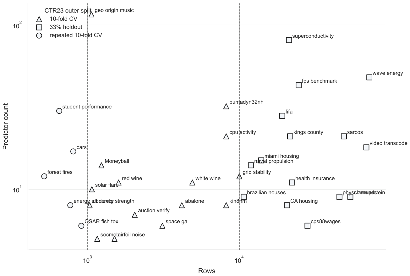
Figure 3.
Rank-distribution profile across the benchmark suite. Each horizontal bar reports how often a model finishes in ranks 1 through 4 across the benchmark tasks. Unlike average rank alone, this view reveals whether a model is consistently near the top or alternates between wins and weak finishes.
Figure 3.
Rank-distribution profile across the benchmark suite. Each horizontal bar reports how often a model finishes in ranks 1 through 4 across the benchmark tasks. Unlike average rank alone, this view reveals whether a model is consistently near the top or alternates between wins and weak finishes.
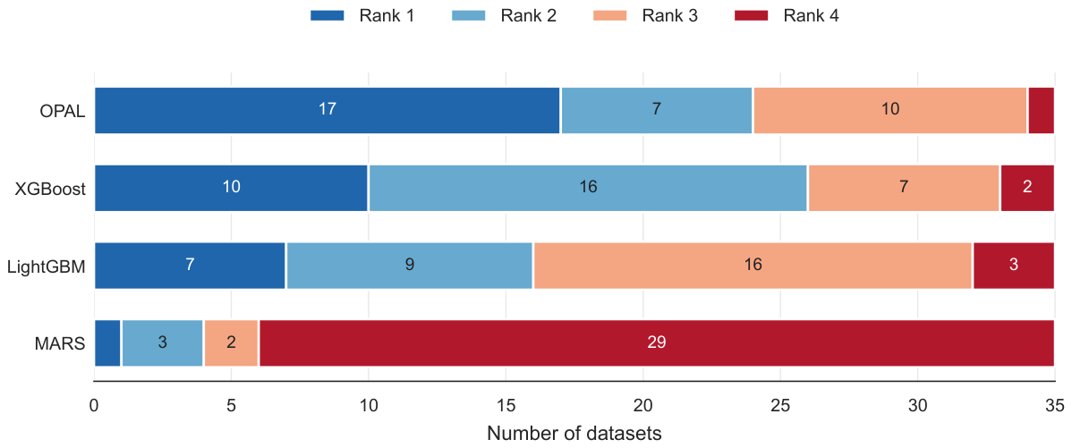
Figure 4.
Model-implied Stage 1 raw-feature contribution curve for education on cps88wages split 9
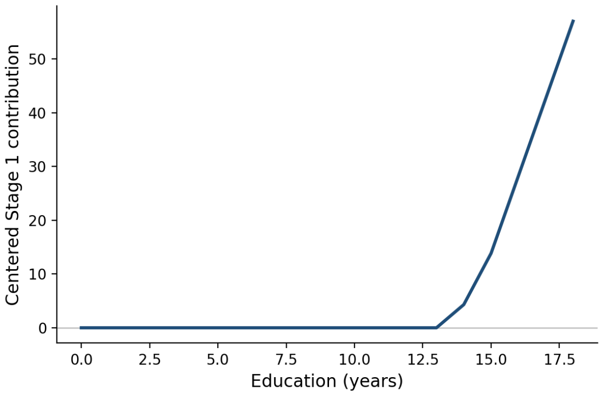
Table 1.
Deterministic numeric transformations available during OPAL feature augmentation.
| Scope | Name | Generated column |
|---|---|---|
| Pairwise | Product | |
| Pairwise | Ratio | |
| Pairwise | Difference | |
| Unary | Signed square root | |
| Unary | Signed logarithm of one plus absolute value | |
| Unary | Square |
Table 2.
OPAL hyperparameter search space used in the benchmark.
| Hyperparameter | Range | Scale |
|---|---|---|
| max_depth | Integer | |
| n_main | Step 75 | |
| n_interact | Step 75 | |
| Logscale | ||
| Logscale | ||
| subsample | Linear | |
| colsample_bytree | Linear | |
| n_quantiles | Step 32 | |
| min_leaf | Integer |
Table 3.
Baseline hyperparameter search spaces used in the benchmark. All ranges are sampled independently by the same 100-trial Optuna random-search protocol used for OPAL.
Table 3.
Baseline hyperparameter search spaces used in the benchmark. All ranges are sampled independently by the same 100-trial Optuna random-search protocol used for OPAL.
| Model | Hyperparameter | Range | Scale |
|---|---|---|---|
| XGBoost | learning_rate | Log | |
| n_estimators | Integer | ||
| max_depth | Integer | ||
| subsample | Linear | ||
| colsample_bytree | Linear | ||
| colsample_bylevel | Linear | ||
| reg_lambda | Log | ||
| reg_alpha | Log | ||
| LightGBM | learning_rate | Log | |
| n_estimators | Integer | ||
| num_leaves | Log-integer | ||
| max_depth | Categorical | ||
| min_child_samples | Log-integer | ||
| subsample | Linear | ||
| subsample_freq | Integer | ||
| colsample_bytree | Linear | ||
| reg_lambda | Log | ||
| reg_alpha | Log | ||
| min_split_gain | Linear | ||
| MARS | max_terms | Step 2 | |
| max_degree | Categorical | ||
| penalty | Log | ||
| thresh | Log |
Table 4.
Aggregate benchmark results across the included four-model panel. Lower average rank, lower median tuning time, and lower geometric mean RMSE ratio are better; the RMSE ratio denominator is the best RMSE among the four evaluated models on the same data set.
Table 4.
Aggregate benchmark results across the included four-model panel. Lower average rank, lower median tuning time, and lower geometric mean RMSE ratio are better; the RMSE ratio denominator is the best RMSE among the four evaluated models on the same data set.
| Model | Datasets | Avg. Rank | First-place | Top-2 | Median tune (s) | Geo. RMSE ratio |
|---|---|---|---|---|---|---|
| OPAL | 35 | 1.8571 | 17 | 24 | 440.9 | 1.0650 |
| XGBoost | 35 | 2.0286 | 10 | 26 | 595.8 | 1.0856 |
| LightGBM | 35 | 2.4286 | 7 | 16 | 612.5 | 1.2505 |
| MARS | 35 | 3.6857 | 1 | 4 | 5.6 | 1.9411 |
Table 5.
Paired OPAL comparisons on overlapping data sets. Negative median relative RMSE indicates lower RMSE for OPAL. Wilcoxon p-values are two-sided unadjusted tests on per-data-set log RMSE ratios.
Table 5.
Paired OPAL comparisons on overlapping data sets. Negative median relative RMSE indicates lower RMSE for OPAL. Wilcoxon p-values are two-sided unadjusted tests on per-data-set log RMSE ratios.
| Comparator | Overlap | Wins / losses | Median RMSE (%) | Log-ratio Wilcoxon p |
|---|---|---|---|---|
| XGBoost | 35 | 19 / 16 | -0.13 | 0.377 |
| LightGBM | 35 | 23 / 12 | -2.01 | 0.018 |
| MARS | 35 | 33 / 2 | -21.19 |
Disclaimer/Publisher’s Note: The statements, opinions and data contained in all publications are solely those of the individual author(s) and contributor(s) and not of MDPI and/or the editor(s). MDPI and/or the editor(s) disclaim responsibility for any injury to people or property resulting from any ideas, methods, instructions or products referred to in the content. |
© 2025 by the author. Licensee MDPI, Basel, Switzerland. This article is an open access article distributed under the terms and conditions of the Creative Commons Attribution (CC BY) license.
Copyright: This open access article is published under a Creative Commons CC BY 4.0 license, which permit the free download, distribution, and reuse, provided that the author and preprint are cited in any reuse.