
Submitted:
13 May 2026
Posted:
14 May 2026
You are already at the latest version
Abstract
To address the problems of strong noise, high asynchrony, pronounced subjectivity in risk labels, and insufficient model stability under extreme market conditions in multi-source risk signals within trading environments, a low-noise investment risk prediction method based on multimodal sensing signals and self-supervised representation learning is proposed. Market quotations, order books, terminal interactions, network transmission, device status, and news sentiment are uniformly modeled as risk perception signals. A temporal masking-based risk structure modeling module, a risk-oriented contrastive learning representation constraint mechanism, and a risk representation and downstream prediction task alignment strategy are designed to learn stable, transferable, and interpretable risk features. Experimental results show that the proposed method achieves the best performance in investment risk prediction, with mean squared error (MSE), mean absolute error (MAE), and root mean square error (RMSE) reaching 0.0164, 0.0851, and 0.1281, respectively, outperforming baseline models including generalized autoregressive conditional heteroskedast (GARCH), multi-layer perceptron (MLP), long short term memory (LSTM), temporal convolutional networks (TCN), and Transformer. The IC, RankIC, and AUC reach 0.496, 0.462, and 0.817, respectively, indicating stronger risk ranking capability and improved discrimination between high-risk and low-risk states. At the classification recognition level, the proposed method also demonstrates superior accuracy, precision, recall, and F1-score, indicating that potential high-risk assets can be identified more accurately. Ablation experiments verify the effectiveness of multimodal fusion, temporal masking, self-supervised contrastive constraints, and task alignment modules. Robustness experiments further show that lower prediction errors and higher AUC can still be maintained in high-volatility and extreme-shock markets, demonstrating strong noise resistance, stability, and practical application potential in complex sensing scenarios.
Keywords:
multimodal sensing
; temporal masking modeling
; multimodal sensor fusion
; time series analysis
; intelligent risk perception systems
1. Introduction
Investment risk prediction and robust modeling are core problems in quantitative investment, asset allocation, portfolio optimization, and systemic risk management, as they directly affect the risk identification, early-warning, and decision-making capabilities of financial institutions and intelligent trading systems [1,2]. Global financial markets are undergoing rapid digital and intelligent transformation, with algorithmic trading and high-frequency trading becoming mainstream paradigms and making price formation, liquidity evolution, and risk transmission more dynamic, complex, and abrupt [3]. Financial data have also evolved from simple price and volume sequences into multi-source heterogeneous information systems composed of order book depth, volatility indices, news texts, sentiment signals, and macroeconomic indicators [4]. These data sources can be regarded as different types of “financial sensors”, jointly reflecting market states at both the micro-level trading layer and the macro-level expectation layer [5]. Therefore, extracting stable, low-noise, and transferable risk features from high-frequency, multimodal, and noisy financial data is of great significance for intelligent investment decision-making and risk management [6].
Traditional investment risk modeling usually quantifies risk through return volatility, value at risk (VaR), conditional value at risk (CVaR), or risk levels, and then constructs supervised learning or statistical modeling tasks [7]. Early methods, such as mean–variance theory, GARCH-type models, historical simulation, and rule-based risk stratification, laid the foundation for financial engineering and improved the standardization of risk analysis [8]. However, these methods are often based on stationarity, linearity, or distributional assumptions, whereas real financial markets exhibit strong non-stationarity, heavy tails, event-driven dynamics, and noise. Consequently, they are prone to failure under high volatility, extreme shocks, and structural changes [9]. More importantly, risk labels are usually not directly observable objective quantities, but are indirectly constructed from specific models, parameter settings, or expert experience, and thus contain subjectivity, bias, and temporal dependence [10]. Once market mechanisms or label distributions shift, models trained on historical labels may suffer performance degradation and insufficient generalization. In multimodal financial scenarios, differences in temporal granularity, statistical distribution, and noise structure further hinder effective cross-modal collaborative modeling.
Deep learning has provided new pathways for financial time-series analysis [11]. Models such as recurrent neural network (RNN), long short term memory (LSTM), and gate recurrent unit (GRU) model temporal dependencies through recurrent structures and show stronger nonlinear fitting ability than traditional statistical models in return prediction, volatility estimation, and trend judgment. Transformer and its variants further improve long-range dependency modeling through self-attention mechanisms [12]. Meanwhile, multimodal fusion learning has been used to jointly model prices, order books, textual sentiment, and macroeconomic indicators to enhance market-state perception [13]. However, most existing deep learning methods still rely on label-intensive supervised learning and large-scale manually defined or derived risk measures, making them vulnerable to label noise and subjectivity. Simple multimodal concatenation or static fusion also struggles with asynchronous alignment, cross-scale dependence, and high-noise interference [14]. In contrast, self-supervised representation learning can extract intrinsic structures from unlabeled data through temporal prediction, masked reconstruction, contrastive learning, and related strategies, offering a potential way to reduce dependence on artificial risk labels and improve robustness and cross-market generalization [15,16]. Gu et al. (2020) [17] and Chen et al. (2024) [18] demonstrated the potential of deep neural networks in stock return and volatility modeling. Contrastive predictive coding (CPC) proposed by Oord et al. (2018) [19] laid a foundation for self-supervised learning on time-series data, and Zhang et al. (2024) [20] reviewed recent advances in this field. Nevertheless, existing studies mainly focus on return prediction or market-state classification, while self-supervised frameworks specifically designed for investment risk representation remain underexplored.
The main contributions of this study are summarized as follows.
- 1.
- Risk prediction is reformulated from a “label-fitting problem” into a “structural representation learning problem”. A low-noise risk feature extraction paradigm that does not rely on strong manually defined risk labels is proposed, thereby alleviating the subjectivity, high construction cost, and noise of risk labels.
- 2.
- Multi-source heterogeneous financial information is comprehensively considered. Price sequences, order books, volatility indices, and news sentiment are uniformly regarded as financial sensing signals, strengthening the perception of the coupling between market micro-level behaviors and macro-level expectations.
- 3.
- A unified modeling mechanism consistent with financial logic is designed to address asynchronous alignment, distribution discrepancies, and multi-scale dependencies in high-frequency financial scenarios, thereby improving robustness and adaptability in complex markets.
- 4.
- Multi-task empirical analysis is conducted to verify the effectiveness, robustness, and interpretability of the proposed method in volatility prediction, VaR estimation, risk ranking, and stability analysis under extreme market conditions.
Methodologically, a low-noise feature extraction framework for investment risk prediction is proposed under a unified paradigm of “multimodal financial sensing fusion + self-supervised risk representation learning”. Financial data from different sources are first independently embedded and encoded, and asynchronous multi-frequency signals are represented in a unified latent space through cross-modal temporal alignment. A temporal masking-based risk structure modeling module is then constructed to learn long-term dependencies and latent uncertainty structures from structurally masked temporal segments. A risk-oriented contrastive learning constraint is further designed, where positive and negative sample pairs are constructed according to financial logic to enhance discrimination across volatility states and risk stages. Finally, a risk representation and downstream task alignment strategy is introduced so that the pretrained risk factors can better support practical tasks such as volatility prediction, estimation, and risk ranking.
2. Related Work
2.1. Investment Risk Prediction and Risk Measurement Methods
Modern portfolio theory regards risk measurement as a core basis for asset allocation and performance evaluation. The mean–variance framework proposed by Markowitz (1952) [1] first quantified return volatility as a risk indicator and enabled the risk–return trade-off through the efficient frontier. The CAPM proposed by Sharpe (1964) [21] decomposed risk into systematic and idiosyncratic components, with beta used to measure market sensitivity. In risk management, VaR was systematically elaborated by Jorion (1997) [22], while CVaR proposed by Rockafellar (2000) [9] provided a more comprehensive description of tail risk. These methods usually construct risk labels from statistical assumptions or subjective parameter settings, implicitly assuming that historical patterns will persist. Deep learning has been increasingly used to predict and extend traditional risk indicators. Gu et al. (2020) [17] used deep feedforward networks and recurrent neural networks to model stock returns, showing the advantages of deep learning in factor discovery and risk prediction. Sezer et al. (2020) [23] reported that CNNs and LSTM outperform traditional machine learning methods in index prediction and foreign exchange trading. Chen et al. (2024) [18] further applied LSTM and Transformer models to volatility modeling and showed the effectiveness of attention mechanisms in capturing long-range dependencies. However, these methods remain supervised paradigms centered on risk labels, and their performance depends heavily on label consistency and reliability. Risk label construction fundamentally limits supervised generalization. When market structures change abruptly, models trained on historical labels often suffer severe degradation. Zitis and Potirakis (2024) [24] indicated that volatility forecasting urgently requires representation learning without strong labels. Huang and Perez (2018) [25] also noted that subjective label differences are a fundamental constraint in anti-money laundering risk scoring.
2.2. Applications of Deep Learning in Financial Time-Series Modeling
Deep learning has reshaped financial time-series modeling. LSTM, as a classical variant of RNN, addresses the vanishing-gradient problem and has become a foundational financial forecasting model. The LSTM framework proposed by Hochreiter and Schmidhuber (1997) [26] was validated by Fischer and Krauss (2018) [27] in stock movement prediction, showing superior out-of-sample performance. Bucci (2020) [28] confirmed the effectiveness of LSTM and GRU in realized volatility forecasting. Transformer models have reshaped sequence modeling through self-attention. The work of Vaswani et al. (2017) [29] inspired many financial applications. Wang et al. (2022) [30] applied deep Transformers to stock index prediction and showed stronger long-range dependency modeling than LSTM. Yañez C et al. (2024) [31] combined variational mode decomposition with Transformer models and improved robustness in non-stationary time-series processing. Ruiru et al. (2025) [32] showed that LSTM–Transformer hybrid architectures can achieve strong performance in multi-asset trading.
Hybrid models have also become important. Sezer et al. (2020) [23] indicated that CNN-LSTM and VMD-GRU outperform single models in many tasks, especially for multi-scale temporal patterns. Chen et al. (2024) [18] summarized deep learning methods for financial time-series forecasting. Based on more than 1 million real financial transactions, Jin and Zhang proposed a stacking model that integrates logistic regression, decision trees, random forests, gradient boosting trees, support vector machines, and neural networks [33]. Rafi et al. compared random forests, gradient boosting, and neural networks on data of a similar scale and combined them with an existing rule-based system, reducing the false positive rate by approximately [34]. Mazumder et al. reconstructed transaction sequences into spatiotemporal matrices and used convolutional neural networks for hierarchical feature extraction from multi-channel structured features [35]. Peddinti et al. reviewed the applications of autoencoders, CNNs, recurrent neural networks , and generative adversarial networks in e-commerce and financial anomaly detection, pointing out that deep models have clear advantages in handling nonlinearity, high dimensionality, and concept drift [36].
However, supervised deep learning still depends on large-scale, high-quality labels. Olorunnimbe and Viktor (2023) [37] pointed out that the low signal-to-noise ratio of financial time series makes label noise severe. Zitis and Potirakis (2024) [24] again emphasized the need for representation learning without strong labels. Ma et al. (2022) [38] analyzed the limitations of fixed-window labeling from a self-supervised perspective, while Song et al. (2026) [39] proposed the “label horizon paradox”, showing that strict alignment between training labels and inference targets is not necessarily optimal.
2.3. Multimodal Fusion and Sensor-Based Anomaly Perception
Multimodal fusion and sensor-based anomaly perception provide an important methodological foundation for complex financial risk modeling. MFGAN proposed by Qu et al. is a representative multimodal anomaly detection framework. This model simultaneously uses distributed control system (DCS) measurement data and acoustic signals, first modeling the temporal dependencies and key features within each modality through an attention-based autoencoder, and then introducing adversarial regularization through GAN to enhance the reconstruction capability for “normal patterns” [40]. Beyond industrial scenarios, multimodal fusion in perception tasks also provides a transferable structure for security perception. MSPE-Fusion proposed by Yu et al. performs multi-level perception enhancement and fusion on sensor features such as radar, LiDAR, and cameras, significantly improving object detection performance [41]. Although this work is mainly designed for autonomous driving, its ideas regarding feature alignment, multi-scale fusion, and attention weight allocation can be transferred to financial scenarios, where trading time series, terminal attributes, geographical locations, and textual logs can be regarded as multi-source sensing information and integrated across modalities through spatiotemporal alignment and attention mechanisms. From a methodological perspective, multimodal fusion techniques were systematically reviewed by Hangloo and Arora, and fusion strategies were summarized into early fusion, intermediate fusion, and late fusion [42]. Existing studies indicate that, in security perception and anomaly detection tasks, multimodal fusion can improve robustness by exploiting redundant information, enabling the system to remain stable even when some modalities are affected by noise or attacks. However, it may also expand the potential attack surface and privacy exposure, especially when sensitive information such as identity, location, and operational behavior is involved.
2.4. Exploration of Self-Supervised and Representation Learning in Financial Scenarios
SSL has achieved major progress in computer vision and natural language processing by learning representations from unlabeled data. In financial applications, SSL has shown potential in denoising, feature robustness, and cross-market generalization. CPC proposed by Oord et al. (2018) [19] laid the foundation for self-supervised learning on time-series data. Sun et al. (2022) [43] proposed Self-FTS to learn latent representations from A-share data through multiple auxiliary tasks, improving trend prediction and portfolio construction. Hwang et al. (2024) [44] proposed SimStock to learn dynamic stock similarities for cross-exchange similar-stock identification and pairs trading. HM Abdulsahib et al. (2024) [45] separated shared and market-specific representations through cross-domain disentangled learning, improving multi-market risk assessment. Duan et al. (2024) [46] proposed MF-CLR for multi-frequency financial data and achieved leading performance in forecasting and classification. DA Nguyen et al. (2024) [47] developed a noise-aware SSL framework for noisy financial time series while maintaining lightweight modeling. However, limitations remain. Giantsidi and Tarantola (2025) [48] reviewed 187 studies and found that most SSL-based financial forecasting studies focus on return prediction or price-direction classification, while investment risk modeling, such as volatility, VaR, and tail risk, remains insufficiently explored.
3. Materials and Method
3.1. Data Collection
The dataset constructed in this study is designed for multi-source hardware sensing-based risk perception tasks in real financial trading environments, with data collection spanning from January 2022 to December 2024. All data are acquired from sensors deployed in trading terminals, network links, edge computing nodes, and trading environments, as shown in Table 1. Specifically, terminal interaction sensing data are collected by touch sensors and inertial measurement sensors deployed on trading workstations and mobile trading devices, primarily recording click frequency, sliding trajectories, input intervals, page dwell time, transaction instruction triggering time, terminal posture changes, and operation response delays, which are used to characterize behavioral variations of traders under different risk states. Network link sensing data are collected by network traffic sensors and link latency sensors deployed at trading network entry points, routing nodes, and edge servers, primarily recording network latency, request frequency, session duration, data transmission intervals, link congestion states, and abnormal access patterns, which are used to reflect the stability of trading links and potential transmission risks.
Device state sensing data are collected by temperature sensors and voltage sensors, primarily recording device temperature, ambient temperature, voltage fluctuations, power supply stability, and hardware operating conditions of trading terminals and edge computing nodes, which are used to identify abnormal risk signals caused by hardware overheating, power anomalies, or performance degradation. Order flow sensing data are collected by order flow intensity sensors and order book depth sensors, primarily recording bid-ask depth, bid-ask spread, order flow intensity, cancellation frequency, transaction triggering time, liquidity variations, and order imbalance, which are used to perceive real-time changes in market microstructure. Trading environment sensing data are collected by environmental temperature and humidity sensors and vibration sensors, primarily recording environmental temperature and humidity variations, vibration intensity around devices, and external physical disturbances, which are used to assist in determining whether external environmental factors affect trading terminals, servers, and network devices. After data collection, all raw data are uniformly processed through sensor identifier binding, timestamp calibration, device state verification, anomaly detection, and missing segment imputation. A unified clock is further adopted to construct multi-frequency time windows, enabling terminal interaction, network link, device state, order flow, and trading environment sensing data to be aligned and fused within a consistent temporal framework.
3.2. Data Preprocessing and Augmentation Strategy
In financial time-series modeling, data preprocessing and temporal augmentation are not merely auxiliary steps before model training, but are critical procedures that directly affect the quality of risk representations and the stability of prediction. The underlying principle is that observed financial market sequences are usually not unbiased and complete expressions of true risk states, but highly noisy observations formed under the joint effects of trading mechanisms, sampling frequencies, market shocks, information transmission delays, and changes in institutional environments. In other words, raw price, return, trading volume, or order flow sequences contain not only effective information reflecting market structures and risk states, but also interference components such as missing observations, abnormal fluctuations, microstructure noise, and distribution drift. Without appropriate preprocessing, these incidental noises may be incorrectly identified by the model as predictive patterns, resulting in overfitting, reduced generalization capability, and unstable performance under extreme market conditions. Therefore, the core objective of data preprocessing is not simply to “clean data”, but to improve the comparability, robustness, and learnability of samples while preserving the economic meaning and dynamic dependency structure of financial time series as much as possible. The core objective of financial temporal augmentation is to perform structurally consistent perturbation and reconstruction of samples without destroying the original economic logic, so that more stable and intrinsic risk representations can be learned from different market scenarios.
Let the original financial time series be denoted as , where represents the d-dimensional observation vector at time t, which may include multiple features such as price, return, trading volume, bid–ask spread, and volatility proxy variables. Since missing values commonly exist in financial data, the completeness of the sequence should first be corrected. For local missing cases in which both preceding and subsequent time points are observable, linear interpolation based on temporal continuity can be adopted to estimate missing values. The basic idea is to use the local trend of adjacent time points to approximate the missing observation, thereby reducing information loss caused by directly deleting samples. If the observation at time t is missing and the nearest valid observations exist at , the interpolation can be expressed as
This method is suitable for short-term missing scenarios because it assumes that changes within adjacent intervals are relatively smooth. For more complex missing patterns in high-frequency financial data, a sliding-window local mean can also be used for robust imputation. Given a window radius of k, the estimate for the missing position t can be written as
where , and denotes the number of valid observations within the window. The principle of this operation is to approximately recover short-term missing segments by using local statistical information, thereby maintaining statistical consistency at the local scale of the sequence. For price-related variables, raw price sequences are usually not directly used. Instead, return transformations are applied to reduce non-stationarity and enhance the model’s perception of relative changes. Let the asset price be denoted as . The simple return can be defined as
whereas the log return, which is more commonly used in financial research, is formulated as
The advantage of log returns lies in their better additivity, making them more suitable for describing continuous compounding and subsequent statistical modeling. For variables with large-scale fluctuations, such as trading volume and bid–ask spread, logarithmic compression or power transformation is often used to weaken the influence of extreme values. For example,
where denotes the original trading volume variable. This transformation can reduce the dominance of large-valued samples in model parameter estimation and improve scale comparability across different samples. Since abnormal fluctuations and heavy-tailed spikes are widely present in financial time series, direct standardization using ordinary mean and standard deviation is easily affected by extreme samples. Therefore, robust standardization is a more reasonable choice. Its basic idea is to replace the mean and standard deviation with the median and interquartile range, thereby obtaining more stable scaling results under skewed or heavy-tailed distributions. Let the sample median of a feature dimension be , and let the first and third quartiles be and , respectively. The robustly standardized result can be expressed as
where is a very small constant used to prevent division by zero. If the data distribution is relatively stable, the classical z-score standardization can also be adopted:
where and denote the sample mean and standard deviation, respectively. However, in high-frequency financial environments, given the frequent changes in local market structures, rolling and robust normalization are emphasized in this study. Let the local mean and local standard deviation within a rolling window of length w be denoted as and , respectively. Dynamic standardization can then be written as
where
This processing strategy can eliminate local scale differences under conditions closer to real trading environments and reduce the interference of long-term institutional changes in model training. To reduce the adverse effects of abnormal fluctuations, extreme observations should also be winsorized or clipped. The principle of this operation is not to deny the existence of extreme market conditions, but to prevent individual abnormal values from exerting disproportionate dominance over parameter learning during training. Let the lower and upper quantile thresholds be denoted as and , respectively, where . The clipped variable can be expressed as
This quantile-based clipping strategy can suppress the influence of extreme values on the estimation of the overall distribution while preserving the ranking relationship among samples as much as possible. If tail events need to be preserved while reducing numerical explosion effects, a hyperbolic tangent compression form can also be adopted:
where is a compression intensity parameter. This method maps values into a bounded interval while retaining positive and negative directional information, thereby improving numerical stability during training. In addition to local missing values and outliers, distribution drift is also prevalent in financial markets. This means that the data-generating mechanism changes across different time periods, leading to distributional inconsistency between the training and testing periods. To address this issue, temporally consistent rolling training should be adopted as much as possible during preprocessing, and detrended or relative expressions should be introduced at the feature level to reduce the influence of long-term drift. For example, for a feature , its relative state can be characterized by the deviation from the local mean:
Furthermore, the local relative change rate can be defined as
so that the model focuses on deviations relative to the recent background rather than absolute levels. This is more consistent with the basic logic of financial risk identification, in which abnormal deviation is regarded as a potential risk signal. After basic preprocessing is completed, the design of financial temporal augmentation strategies should follow the principle that perturbations should not destroy economic semantics. Unlike computer vision, where general augmentation operations such as random cropping and color perturbation can be directly used, every change in financial time series corresponds to potential market meaning. Therefore, augmentation operations must serve the learning of more robust risk structures rather than generating pseudo-samples lacking realistic interpretation. First, temporal window cropping augmentation can be adopted, in which continuous subsequences with slightly different lengths are extracted from the original sample, allowing the model to identify consistent risk states under different observation windows. Let the original sequence segment be , the cropping length be , and the starting point be s. The augmented sample is then defined as
The rationale behind this operation is that, in real trading decisions, investors usually cannot observe a completely identical fixed window, but instead make judgments based on historical information of varying lengths. Therefore, window cropping can improve the model’s adaptability to changes in observation scope. Second, amplitude scaling augmentation can be used to simulate volatility processes with similar patterns under different levels of market activity. If the return sequence is scaled, the augmented result can be written as
where is a scaling coefficient close to 1, usually set as , and is a small positive value. The essence of this operation is to simulate the manifestation of the same risk structure under different volatility intensities, enabling the model to focus on the volatility pattern itself rather than relying only on absolute magnitude. Unlike completely random noise injection, this transformation preserves the sign of returns, relative trends, and temporal dependencies, and thus has strong financial rationality. Third, local temporal jittering can be used to simulate slight shifts in information arrival time, which is particularly suitable for multimodal alignment scenarios. If the time index of a subsequence is shifted by no more than , the augmented sample can be expressed as
Here, should usually satisfy local smoothness or piecewise-constant constraints to avoid completely disrupting the temporal order. This augmentation method reflects the slight time lags that commonly exist among news releases, order book responses, and price reactions in real financial systems, thereby improving the model’s tolerance to asynchronous financial sensing signals. In addition, state-consistent segment replacement augmentation based on economic conditions is emphasized in this study. Let two sample segments be denoted as and . If they exhibit high similarity under a certain state indicator, such as similar local volatility, the corresponding segment in can be used to replace part of , yielding the augmented sample
To ensure the rationality of replacement, local volatility can be used as a similarity metric. Let the return sequence within window W be denoted as . The local volatility can then be defined as
where is the average return within the window. Replacement is performed only when the two segments satisfy
where is the similarity threshold. The significance of this strategy lies in extracting and splicing local structures from different samples under similar risk states, thereby enhancing the model’s ability to understand the financial fact that similar states may correspond to different individual paths. In self-supervised or contrastive learning scenarios, two different augmented views are usually constructed for representation consistency constraints. Let the original sample be denoted as X, and let two financially logical augmented samples be denoted as and . The encoder outputs the representations and . Their consistency can then be constrained through a similarity objective, such as cosine similarity, defined as
This setting indicates that samples augmented under consistent economic semantics should remain close in the representation space, thereby encouraging the model to learn risk features that remain stable across noise and local perturbations.
3.3. Proposed Method
3.3.1. Overall
The proposed method is constructed as a unified framework consisting of “multimodal financial sensing encoding–temporal masking-based self-supervised modeling–risk-contrastive representation constraint–downstream task-aligned prediction”. Given multi-source financial samples that have been temporally aligned and feature-normalized, different modalities, including market quotations, order book structures, terminal interactions, network transmission, device status, and news sentiment, are first fed into their corresponding modality encoders. For continuous temporal modalities, temporal convolution and attention-based encoding structures are adopted to extract local volatility patterns and long-range dependencies. For textual sentiment modalities, semantic encoders are used to capture event shocks and market expectation information. Subsequently, modality-specific features are mapped into a unified latent space, and the importance weights of different modalities under the current market state are calculated through a cross-modal attention fusion module, thereby forming a comprehensive risk-state representation. This representation is not directly fed into a supervised predictor, but is first introduced into the self-supervised risk representation learning stage. In this stage, several key temporal segments in the input sequence are masked, forcing the encoder to reconstruct the masked content based on unmasked price movements, order book changes, interaction behaviors, network states, and sentiment signals. In this way, intrinsic dependencies and latent risk structures across different temporal segments can be learned. The contextual representation output by the temporal masking module is further fed into the risk-oriented contrastive learning module. Positive and negative sample pairs are constructed according to local volatility, order book imbalance, sentiment shock intensity, and risk-stage similarity, so that samples under similar risk states are pulled closer in the representation space, whereas samples under different risk states are effectively separated. Consequently, the interference of short-term noise and incidental fluctuations in representation learning can be reduced. After self-supervised pretraining is completed, the learned low-noise risk representation is transferred to the downstream task alignment module. Corresponding prediction heads are designed for different investment risk tasks, including future volatility regression, estimation, risk-level classification, and asset risk ranking, so that the general risk representation can be matched with specific investment decision-making objectives. During the overall training process, the masked reconstruction objective is used to constrain the model to learn temporal structures, the contrastive learning objective is used to optimize the risk representation space, and the downstream task objective is used to calibrate predictive value. These three objectives jointly enable stable, transferable, and interpretable investment risk features to be extracted from multimodal financial sensing signals.
3.3.2. Temporal Masking-Based Risk Structure Modeling Module
The temporal masking-based risk structure modeling module follows a self-supervised learning process of “masked input–encoded representation–decoded reconstruction–structural constraint”. Its core objective is to guide the model to learn stable long-term risk structures from multimodal financial sensing sequences without relying on manually defined risk labels. Let the aligned input sequence be denoted as , where represents the multimodal financial state vector at time t, containing features such as market quotations, order books, terminal interactions, network states, device status, and sentiment signals. First, a binary mask vector is generated according to the masking strategy, and the masked input is obtained as , where denotes a learnable mask embedding. Unlike ordinary random masking, the masking units in this study mainly consist of continuous temporal segments, and risk-related indicators such as local volatility, order book imbalance, and abnormal interaction intensity are incorporated to adjust the masking probability, making high-uncertainty regions more likely to be masked. This design forces the model to recover missing information according to market states before and after the masked segments, cross-modal collaborative relationships, and long-term temporal dependencies, thereby preventing the model from merely memorizing local noise or short-term price spikes.
As shown in Figure 1, from the perspective of network structure, the masked sequence is first fed into the temporal encoder to obtain the contextual latent representation . The encoder consists of a modality embedding layer, a positional encoding layer, and multiple temporal attention blocks. The modality embedding layer projects sensing signals from different sources into a unified dimension , the positional encoding layer is used to preserve the temporal order of financial sequences, and the temporal attention block calculates dependencies among different temporal segments through query, key, and value mappings. Its basic form is given by . Through this structure, associations between masked and unmasked segments can be established over the global temporal range, while short-term volatility shocks and long-term risk accumulation processes can be captured simultaneously. Subsequently, the latent representation H is fed into the decoder to reconstruct the original observations at the masked positions, yielding . A lightweight multilayer perceptron or reverse temporal attention structure is adopted as the decoder to prevent excessive model capacity from directly copying input noise. The reconstruction loss is calculated only at the masked positions and can be expressed as , where denotes the set of masked temporal indices. For risk-sensitive variables such as volatility, bid–ask spread, and latency, a weighted reconstruction form can also be introduced as , where is determined by local risk intensity, enabling the model to focus more on temporal segments with significant risk-state changes.
From a mathematical perspective, temporal masking modeling is essentially intended to maximize the conditional dependence between masked segments and contextual segments, namely to learn . In highly noisy financial environments, random micro-level perturbations are often difficult to predict stably from context, whereas risk states jointly determined by market structure, liquidity changes, and sentiment shocks possess stronger conditional recoverability. Therefore, when the model is required to recover masked segments from context, structurally consistent risk factors are more likely to be preserved, while the influence of unpredictable noise is weakened. This module is also connected to the subsequent contrastive learning branch. The latent representation output by the encoder is fed into the reconstruction decoder to calculate the reconstruction constraint on the one hand, and is used as the risk representation input to the projection layer for consistency constraints with augmented-view representations on the other hand. Therefore, the model can learn not only how to recover masked financial states, but also which structures remain stable under different perturbations. This design is particularly suitable for the investment risk prediction task in this study, because risk is usually not a single-point anomaly but the result of the gradual accumulation of multimodal signals over time. Through masked reconstruction, dynamic transmission relationships among price volatility, order book liquidity, terminal interactions, and external sentiment can be explicitly modeled, thereby yielding low-noise, transferable, and more interpretable risk structure representations.
3.3.3. Risk-oriented Contrastive Learning Representation Constraint Mechanism
The risk-oriented contrastive learning representation constraint mechanism adopts a “dual-branch encoding–projection–similarity constraint” structure. However, its design focus is not arbitrary augmentation of original samples, but the construction of multi-view representations with economic equivalence around financial risk states.
As shown in Figure 2, let the input multimodal financial risk sequence be denoted as , where T represents the temporal length and C represents the number of fused channels. First, a set of risk-equivalent transformations is constructed for the original sequence, corresponding to local temporal perturbation, amplitude-preserving scaling, frequency-domain low-noise enhancement, and empirical mode decomposition reconstruction, respectively. After transformation, multiple risk-consistent views are obtained, while the original view is retained. These views differ in short-term noise, local amplitude, or frequency-domain details, but their latent risk states should remain consistent; thus, they are defined as positive sample relationships. Each augmented view is fed into the shared-parameter risk encoder , while the original view is fed into the baseline encoder , which has an independent but structurally identical architecture. The encoder consists of one-dimensional temporal convolution blocks, multi-head temporal attention blocks, and a global risk pooling layer. The input size of the l-th convolution block is , the kernel size is , the stride is , and the output channel number is . Therefore, the output width can be expressed as , and the output feature is denoted as . Subsequently, the attention layer maps risk dependencies along the temporal dimension into the latent dimension D, and the output representation is denoted as . To prevent contrastive learning from directly constraining backbone features and impairing downstream predictive capability, the encoded result is further fed into the projection head . The projection head consists of fully connected layers, with the width of the j-th layer denoted as , and the final output is . This design allows the backbone encoder to retain interpretable risk factors, while the projection space mainly undertakes contrastive optimization. For any original sample , its original representation and augmented representation are respectively defined as
To make the similarity constraint more consistent with financial logic, an ordinary instance-level contrastive loss is not directly adopted. Instead, risk-state weights are introduced. Let the risk-state statistics of samples i and j be denoted as and , respectively, which may include local volatility, order book imbalance, tail-loss intensity, and sentiment shock intensity. The risk-consistency weight between them is then defined as
where is the smoothing parameter for risk-state similarity. When the risk states of two samples are closer, becomes larger, and the model tends to pull them closer in the representation space. Furthermore, the risk-oriented contrastive objective between the augmented views and the original view can be formulated as
where denotes normalized inner-product similarity and denotes the temperature coefficient. Unlike ordinary contrastive learning, this loss does not simply distinguish sample identities, but adjusts positive and negative sample boundaries through risk-state similarity, enabling the model to focus more on whether the risk structures are consistent rather than whether the samples originate from the same temporal window. The mathematical rationality of this design can be explained from the perspective of representation invariance. If the risk-equivalent transformation does not change the latent risk variable , namely , the ideal encoder should satisfy
When is minimized, the positive sample term increases , and the following constraint tendency can therefore be obtained:
Meanwhile, for samples with large differences in risk states, a larger forms a stronger separation boundary in the denominator, encouraging the representations to satisfy
where is a margin function that increases with risk-state differences. Accordingly, this module constructs a risk-aware metric structure in the representation space. Multiple perturbed views under the same risk semantics are compressed into adjacent regions, while samples from different risk stages are pushed farther apart. When applied to the task in this study, this mechanism can effectively reduce the interference of random noise, local spikes, and asynchronous sensing errors in high-frequency financial data during representation learning. The model no longer relies on a single price pattern, but extracts risk factors from multimodal sensing signals that remain stable across windows, assets, and markets. Compared with a self-supervised objective that relies only on masked reconstruction, the risk-oriented contrastive constraint further enhances the discriminability of the representation space, allowing subsequent volatility prediction, estimation, and risk ranking tasks to obtain clearer, lower-noise, and economically interpretable input features.
3.3.4. Risk Representation and Downstream Prediction Task Alignment Strategy
The risk representation and downstream prediction task alignment strategy adopts a hierarchical design of “shared risk encoding–learnable mapping–mixture-of-experts prediction” in its overall structure, enabling the general risk representation obtained in the self-supervised stage to be effectively transformed into task-specific features required for investment decision-making. As shown in Figure 3, let the unified risk representation obtained from the preceding modules be denoted as . It is first fed into the embedding network for feature compression and reconstruction, yielding the basic embedding vector . The embedding network consists of multiple linear transformations and nonlinear activations, and the width of each layer is denoted as . Through layer-wise projection, high-dimensional risk factors are mapped into a compact task space. Subsequently, a learnable mapping module is introduced to structurally transform the intermediate features, which can be expressed as
where denotes the transformation matrix and denotes the nonlinear activation function. This module is used to eliminate the distributional shift between self-supervised representations and downstream tasks, making the risk factors semantically closer to the prediction targets.
In the prediction stage, a risk prediction network based on a mixture-of-experts mechanism is adopted to improve the adaptability of the model under different market states. Let several sub-prediction experts be denoted as . Each expert is used to model a specific risk pattern, such as a high-volatility phase, liquidity shock phase, or sentiment-driven phase. Its output is given by
where is composed of a multilayer feedforward network, and the hidden dimension of each layer is denoted as . Complex risk patterns can therefore be captured through nonlinear mapping. To dynamically select the most appropriate expert, a gating network is constructed to generate expert weights according to the current risk representation:
where denotes the gating function. The final prediction is obtained as a weighted combination of the outputs of all experts:
From a mathematical perspective, this structure is equivalent to decomposing the conditional distribution as
where is produced by the gating network, and is modeled by the corresponding expert. This decomposition can effectively characterize the property that different risk states in financial markets correspond to different generation mechanisms. When the market is in different phases, the gating network automatically adjusts the expert weights, enabling the model to select the most appropriate risk pattern for prediction and thus avoiding the limitation that a single model is difficult to adapt to changing environments. To achieve effective alignment between representations and tasks, a joint optimization objective is introduced during training, so that the risk representation not only satisfies self-supervised structural constraints but also minimizes the downstream task loss . The overall optimization objective can be written as
where denotes the self-supervised loss from the preceding modules, and is the trade-off coefficient. This objective ensures that the encoder gradually adjusts the representation space to downstream prediction tasks while preserving general structural information. This design offers several advantages for the task in this study. First, through the embedding and learnable mapping modules, self-supervised risk representations are effectively transformed into a feature space with task semantics, thereby avoiding misalignment between representations and prediction targets. Second, the mixture-of-experts structure can characterize the diversity of financial risks, allowing the model to automatically select the optimal prediction path under different market states and thus improving robustness and generalization capability. Finally, the gating mechanism enables dynamic adaptability. When facing high-frequency noise, structural breaks, and cross-market transfer, the model can adjust its decision logic according to the current risk state, thereby achieving more stable and accurate investment risk prediction.
4. Results and Discussion
4.1. Experimental Configuration
4.1.1. Hardware and Software Platform
In terms of the hardware platform, all experiments were conducted on a high-performance deep learning workstation. The server-side processor was an Intel Xeon Silver-series multi-core CPU with a clock frequency of no less than , which was used to support large-scale financial time-series data loading, feature preprocessing, and parallel training tasks. The graphics processing unit was an NVIDIA RTX 4090 or an equivalent GPU with of memory, which satisfied the batch training and attention computation requirements of multimodal financial sequences under the Transformer framework. The system memory was configured as to ensure efficient caching and fast access to high-frequency order book data, price sequences, textual sentiment signals, and macroeconomic indicators during joint modeling. Local storage was provided by a NVMe SSD to improve the read-and-write efficiency of high-frequency financial data slicing, model parameter saving, and experimental log recording. The overall hardware platform provided sufficient support for training and validating the proposed model in multi-asset, high-frequency, and multimodal financial scenarios, while ensuring experimental stability and reproducibility. In terms of the software platform, the experiments were implemented on the Ubuntu 22.04 LTS operating system. PyTorch 2.2 was adopted as the deep learning framework, and CUDA 12.1 and cuDNN acceleration libraries were used during model training to improve the computational efficiency of tensor operations and attention modules. Python 3.10 was used as the programming language. Data processing mainly relied on NumPy, Pandas, and SciPy for financial time-series cleaning, sliding-window construction, and statistical feature calculation. Technical indicator generation and experimental analysis were implemented with Scikit-learn, while model visualization and result plotting were performed using Matplotlib and Seaborn. To ensure the consistency of experimental results, random seeds were fixed during training, and pseudo-random number generation states, deterministic GPU operation options, and logging modules were uniformly configured in the software environment, thereby reducing result fluctuations caused by differences in the running environment.
In terms of dataset partitioning and hyperparameter settings, the samples were divided in chronological order to avoid future information leakage. The overall dataset was divided into training, validation, and test sets at a ratio of , where the training set was used for model parameter learning, the validation set was used for model selection and early stopping control, and the test set was used for final performance evaluation. Considering the significant stage-wise characteristics and distribution drift of financial markets, a 5-fold cross-validation strategy was further adopted during training. Specifically, 5 rolling subsets were constructed within the training samples in chronological order, and model training and validation were alternately performed to more robustly evaluate the generalization capability of the model across different market phases. The input temporal window length was set to , indicating that the model used historical information from 60 consecutive time steps to predict future risk states. The embedding dimension was set to , the number of multi-head attention heads was set to , the number of Transformer encoder layers was set to 3, and the hidden dimension of the feed-forward network was set to 256. AdamW was used as the optimizer, with the initial learning rate set to , the weight decay coefficient set to , the batch size set to 32, and the maximum number of training epochs set to 100. Early stopping was triggered when the validation performance did not improve for 10 consecutive epochs. To enhance training stability, the dropout rate was set to , and the gradient clipping threshold was set to . In the self-supervised pretraining stage, the temporal masking ratio was set to , the contrastive learning temperature parameter was set to , and the weight coefficient of the alignment loss between risk representations and downstream tasks was set to . These parameter settings comprehensively considered the strong noise, sharp local fluctuations, and high computational complexity of multimodal fusion in high-frequency financial data, thereby maintaining model expressiveness while controlling training costs and improving robustness and adaptability in real-world investment risk prediction tasks.
4.1.2. Baseline Models and Evaluation Metrics
The baseline models included GARCH [49], LSTM [50], MLP [51], Transformer [29], and TCN [52]. GARCH is a classical financial volatility modeling method that characterizes time-varying volatility clustering in return sequences through the dynamic recursion of conditional variance. Its advantage lies in strong financial interpretability and its ability to reflect the statistical evolution of risk over time. LSTM is a recurrent neural network based on gating mechanisms, which can retain historical information over relatively long temporal ranges in sequence modeling and is suitable for capturing dynamic dependencies in financial time series. Its advantage lies in its strong ability to learn nonlinear temporal features. MLP is a feed-forward fully connected neural network that usually takes multidimensional financial features within a sliding window as flattened inputs for supervised learning. Its advantages are structural simplicity and stable training, making it suitable as a basic comparison model without complex temporal modeling or pretraining mechanisms. Transformer is a time-series modeling method based on the self-attention mechanism, which can directly model global dependencies among different temporal positions. Its advantage lies in its strong capability to capture long-range dependencies, making it suitable for high-dimensional and multivariate financial time-series data. TCN expands the receptive field through causal and dilated convolutions while maintaining temporal causality, thereby effectively modeling dynamic patterns across different temporal scales. Its advantage lies in high parallel computational efficiency and generally stable performance in medium- and long-sequence prediction tasks.
Based on the practical requirements of investment risk management, mean squared error (MSE), mean absolute error (MAE), root mean squared error (RMSE), information coefficient (IC), rank information coefficient (RankIC), and the classification discrimination metric AUC were selected as evaluation metrics. Among them, MSE, MAE, and RMSE were used to measure the prediction accuracy of continuous risk values; IC and RankIC were used to characterize the model’s ability to rank risk magnitudes; and AUC was used to evaluate the model’s ability to distinguish between high-risk and low-risk states. The definitions of the relevant metrics are as follows:
where N denotes the number of samples, denotes the true risk value of the i-th sample, denotes the predicted value of the model, and denote the sample means of the true and predicted values, respectively, denotes the rank difference between the true ranking and predicted ranking of the i-th sample, denotes the true positive rate, denotes the false positive rate, and u is the integration variable. In practical computation with discrete approximation, AUC can be understood as the area under the ROC curve.
4.2. Performance Comparison of Different Models
This experiment was designed to verify the effectiveness of the proposed method in investment risk prediction from three perspectives: overall prediction accuracy, risk ranking capability, and discrimination between high-risk and low-risk states.
As shown in Table 2 and Figure 4, GARCH achieved MSE, MAE, and RMSE values of , , and , respectively, while its IC, RankIC, and AUC values were , , and , respectively, indicating the weakest overall performance. This result suggests that although traditional conditional heteroskedasticity models can characterize volatility clustering, they are difficult to adapt to multimodal, high-noise, and strongly nonlinear financial risk scenarios. MLP showed a certain improvement over GARCH, with MSE reduced to and AUC increased to , indicating that nonlinear mapping can enhance the fitting ability of risk features. However, due to the lack of explicit temporal structure modeling, it remains difficult for MLP to fully capture the dynamic accumulation and transmission process of risk over time. The errors of LSTM were further reduced, with IC and RankIC improved to and , respectively, indicating that the gated recurrent structure can retain certain historical information and effectively model dynamic dependencies in financial time series. TCN performed slightly better than LSTM, with an MSE of and an AUC of , suggesting that causal convolution and dilated convolution can enlarge the receptive field while preserving temporal order, thereby providing more stable modeling of multi-scale volatility patterns. Transformer achieved the best performance among all baseline models, with MSE reduced to and and AUC reaching and , respectively, indicating the advantages of self-attention mechanisms in capturing long-range dependencies and multivariate interactions.
The proposed method achieved the best results across all evaluation metrics, with MSE, MAE, and RMSE reaching , , and , respectively, which were clearly lower than those of all baseline models. Meanwhile, IC, RankIC, and AUC increased to , , and , respectively, indicating that the proposed method can not only predict continuous risk values more accurately, but also more effectively distinguish asset risk magnitudes and high-risk versus low-risk states. Theoretically, GARCH mainly relies on a predefined conditional variance recursion and is essentially a low-dimensional statistical assumption-based model; therefore, its expressive capability is limited under market structural breaks and nonlinear risk transmission. Although MLP has universal function approximation capability, flattening the temporal window tends to weaken temporal order information. LSTM mitigates long-term dependency issues through gating mechanisms, but recursive propagation may still lead to information attenuation. TCN captures local-to-medium-term patterns through convolutional receptive fields, but its ability to express global cross-modal dependencies remains limited. Transformer can model global correlations through attention weights, but it is easily disturbed by local abnormal fluctuations in highly noisy financial data. In contrast, the proposed method further introduces multimodal financial sensing fusion, temporal masking-based self-supervised learning, risk-oriented contrastive constraints, and downstream task alignment on the basis of Transformer-like global modeling capability. As a result, more stable latent risk structures can be extracted from noisy observations, and the discriminability of the representation space can be enhanced through risk-semantic consistency constraints. Therefore, stronger comprehensive advantages are achieved in error control, ranking consistency, and risk-state identification.
4.3. Ablation Study
This ablation experiment was designed to verify the actual contribution of each core module to the overall performance and to determine whether the performance improvement was derived from the synergistic effect of multiple modules in the complete framework rather than from an increase in network scale alone.
As shown in Table 3 and Figure 5, the most pronounced performance degradation occurred after removing the multimodal fusion module, with MSE increasing to and AUC decreasing to . This indicates that reliance on a single or weakly fused financial signal is insufficient for characterizing complex market risks. After the temporal masking module was removed, the MSE reached , while IC and RankIC decreased to and , respectively, suggesting that the absence of self-supervised masked reconstruction weakened the model’s ability to learn long-term risk structures and contextual dependencies. After removing risk-oriented contrastive learning, the model obtained an MSE of and an AUC of , demonstrating the importance of contrastive constraints for distinguishing risk states. When the task alignment strategy was removed, model performance also declined, with an MSE of and an AUC of , indicating that self-supervised representations may still deviate from actual prediction requirements if they are not calibrated by downstream risk objectives. The complete model achieved the best results across all metrics, with MSE, MAE, and RMSE values of , , and , respectively, and IC, RankIC, and AUC values of , , and , respectively, verifying the effectiveness and complementarity of all modules.
From a theoretical perspective, the multimodal fusion module maps market quotations, order books, terminal interactions, network states, device status, and sentiment information into a unified risk space, enabling the model to exploit complementary relationships among signals from different sources. Therefore, removing this module weakens the completeness of risk perception. The temporal masking module essentially learns the conditional dependencies within financial sequences through contextual reconstruction constraints, allowing the model to focus more on stable risk factors explainable by long-term structures rather than short-term noise. Thus, the absence of this module reduces the low-noise property of the learned representations. Risk-oriented contrastive learning optimizes the geometric structure of the representation space by pulling similar risk states closer and separating different risk states; therefore, its removal weakens the model’s ability to distinguish high-risk and low-risk samples. The task alignment strategy transforms general self-supervised representations into task-specific features suitable for volatility prediction, VaR estimation, and risk ranking through learnable mapping and a mixture-of-experts prediction mechanism. Consequently, removing this strategy reduces the matching degree between predicted values and actual risk objectives. The complete model achieves the best performance because masked modeling provides structural stability, contrastive learning enhances risk discriminability, multimodal fusion ensures information completeness, and task alignment maintains consistency with prediction objectives. These components jointly reduce the influence of high-frequency financial noise and market non-stationarity on the model.
4.4. Robustness Comparison
This experiment was designed to evaluate the stability and generalization capability of different models under changing market conditions, with a particular focus on the degree of performance degradation when the market shifts from normal conditions to high-volatility and extreme-shock conditions.
As shown in Table 4 and Figure 6, LSTM, Transformer, and the proposed method all achieved relatively stable prediction results under normal market conditions. Transformer showed certain advantages over LSTM in terms of error and ranking metrics, while the proposed method further achieved the best results, indicating strong risk modeling capability under regular market conditions. When the market entered a high-volatility state, the errors of all models increased significantly. The MSE of LSTM increased from to , and that of Transformer increased to , whereas the proposed method increased only to . Meanwhile, the decreases in IC and AUC were also substantially smaller than those of the baseline models. Under extreme-shock market conditions, this difference became more evident. The errors of LSTM and Transformer further expanded, and their ranking capability declined noticeably, whereas the proposed method still maintained relatively low errors and high discrimination capability, indicating stronger adaptability to abnormal market environments.
From the perspective of model mechanisms, LSTM relies on a recurrent structure to transmit historical information step by step. Its memory mechanism can effectively capture local dependencies in stable environments, but under high volatility or sudden shocks, accumulated historical information often contains substantial noise, which leads to error amplification and reduced discrimination capability. Although Transformer can model long-range dependencies through a global attention mechanism, its attention weight distribution is easily disturbed by abnormal fluctuations in high-noise environments, causing the model to overreact to extreme samples and thereby affecting overall stability. In contrast, the proposed method uses a self-supervised temporal masking mechanism to encourage the model to learn structural risk factors that can be stably recovered from context, thereby suppressing random noise at a fundamental level. Meanwhile, the risk-oriented contrastive learning constraint strengthens the separation among different risk states in the representation space, allowing the model to maintain clear risk boundaries under distributional changes. The introduction of multimodal information further provides cross-source redundant signals, which helps mitigate the influence of distortion from a single data source. Therefore, in a mathematical sense, the proposed method reduces the sensitivity of outputs to input perturbations by constraining the stability and discriminability of the representation space, enabling better predictive performance under distribution drift and extreme events.
4.5. Sensor Sensitivity Analysis
To further evaluate the contribution of different types of sensors to the investment risk perception task, a sensor sensitivity analysis experiment was designed. Specifically, based on the complete model, one type of sensor data was removed at a time, while the remaining sensing signals were retained for model training and testing, so that changes in model performance could be observed. In this way, the influence of each type of sensor on risk prediction results can be quantitatively analyzed, and the necessity of multi-source sensor fusion can be verified.
As shown in Table 5, significant differences are observed in the contributions of different sensor types to model performance. First, after the order flow sensors were removed, the most pronounced performance degradation was observed, with increasing to and decreasing to . This indicates that microstructure information, such as order flow intensity and order book depth, constitutes a core source for risk identification. Such sensing signals can directly reflect market liquidity changes and trading behavior imbalance, which are key precursors to risk formation. Second, the removal of network link sensors and terminal interaction sensors also led to substantial performance degradation, indicating that trading latency, request frequency, and user operation behavior play important roles in risk perception. This suggests that risk is not only derived from the market itself, but is also closely related to the state of the trading system and participant behavior. In contrast, device state sensors and trading environment sensors had relatively smaller effects on model performance, but still provided stable performance gains, suggesting that their main role is to filter noise introduced by hardware anomalies or external environmental interference, thereby improving model robustness. From an overall perspective, this experiment verifies the necessity of multi-source sensor fusion in financial risk perception. A single type of sensor can only provide partial information, whereas risk formation is usually the result of multi-factor coupling. Order flow sensors provide market microstructure information, terminal and network sensors provide trading behavior and system state information, and device and environment sensors provide noise suppression and anomaly detection capabilities. Through collaborative modeling of multi-source sensors, risk signals can be captured across different dimensions, and stable performance can be maintained in high-noise and non-stationary environments.
4.6. Discussion
The practical value of the proposed method is mainly reflected in real financial trading and risk management scenarios. For securities firms, fund companies, and quantitative investment institutions, investment risk does not only arise from short-term price fluctuations, but is often driven by the joint effects of multiple factors, including sudden declines in order book liquidity, abnormal trading terminal behavior, increased network latency, news-event shocks, and rapid reversals in investor sentiment. By incorporating these multi-source signals into a unified financial risk perception framework, the proposed method can more closely approximate the actual risk formation mechanism in real trading processes. For example, in high-frequency trading scenarios, before a stock experiences a substantial price decline, early signs may already appear, such as reduced bid–ask depth, widened spreads, increased order cancellation frequency, and concentrated abnormal network requests. Traditional models that rely only on historical returns or volatility often respond only after risk has become explicit. In contrast, the proposed method can capture these implicit changes in advance through multimodal risk representations, thereby providing earlier risk warning signals for trading systems. The proposed method also has strong application significance in portfolio management. When asset allocation is performed by fund managers or intelligent advisory systems, it is necessary not only to judge whether a single asset may face high volatility in the future, but also to compare the relative risk levels among different assets. The improvements in IC and RankIC indicate that the proposed model can more accurately characterize asset risk ranking relationships, which is directly valuable for portfolio weight adjustment, position control, and risk budget allocation. For instance, when the market enters a period of high policy uncertainty or intensive macroeconomic data releases, the model can dynamically rank the risk exposures of different assets by integrating price trends, volatility changes, news sentiment, and trading behavior signals. This can assist investors in reducing the weights of high-risk assets and increasing allocations to lower-risk or more stable assets. Such an application does not simply pursue return prediction, but places greater emphasis on drawdown control and portfolio stability in complex market environments. In addition, in trading risk control and anomaly monitoring scenarios, the proposed method can provide more fine-grained perception capability for real-time risk monitoring systems. In actual trading, extreme market conditions are often not triggered by a single factor, but are jointly driven by liquidity deterioration, market sentiment diffusion, and crowded trading behavior. Through temporal masking modeling and risk-oriented contrastive learning, the proposed method can identify relatively stable structural features under different risk states and maintain reliable judgment even when market noise is strong. For example, after the release of sudden negative news, if order book imbalance, intensive terminal trading instructions, and significant deterioration in market sentiment are simultaneously detected, the model can identify the corresponding asset as a short-term high-risk target and assist the system in triggering risk alerts, reducing trading frequency, or adjusting stop-loss thresholds. Therefore, the proposed method is not only applicable to offline risk assessment, but can also be embedded into intelligent trading terminals, securities firm risk control platforms, and quantitative investment systems to provide more stable, interpretable, and actionable risk perception support for real investment decision-making.
4.7. Limitation and Future Work
Several limitations remain in this study. First, although the constructed multimodal financial risk perception data cover market quotations, order books, terminal interactions, network states, device status, and news sentiment, the data sources are still mainly concentrated in specific markets and time periods. The applicability of the model to more national markets, different asset classes, and longer periods still requires further validation. Second, frequency differences and time delays exist between hardware sensing data and financial trading data. Although temporal alignment was performed in this study, asynchronous errors in extremely low-latency scenarios may still affect model judgment in real high-frequency trading environments. Third, although self-supervised representation learning and multimodal fusion mechanisms improved predictive performance, they also increased model complexity and imposed higher requirements on computational resources and deployment environments. Future work will further expand data sources by introducing more markets, asset classes, and cross-period samples to verify the stability of the model under cross-market transfer and extreme market conditions. Meanwhile, lightweight deployment schemes can be further optimized, making the model more suitable for integration into securities firm risk control platforms, quantitative trading systems, and edge computing devices. In addition, subsequent studies may strengthen model interpretability analysis to further clarify the contribution mechanisms of different sensing signals in risk warning.
5. Conclusion
To address the problems of complex risk signal sources, strong noise, obvious asynchrony, and unstable manually defined risk labels in trading environments, a low-noise investment risk prediction method based on multimodal sensing signals and self-supervised representation learning is proposed. Market quotations, order books, terminal interactions, network transmission, device status, and news sentiment are uniformly modeled as risk perception signals, and more stable, transferable, and interpretable risk representations are extracted through temporal masking modeling, risk-oriented contrastive learning, and downstream task alignment strategies. Experimental results show that the proposed method achieves the best overall performance in investment risk prediction, with , , and reaching , , and , respectively, clearly outperforming baseline models such as GARCH, MLP, LSTM, TCN, and Transformer. Meanwhile, , , and reach , , and , respectively, indicating that the model has advantages in risk ranking, high-risk and low-risk discrimination, and classification recognition capability, while also reflecting better accuracy, precision, and recall performance. Ablation experiments further demonstrate that multimodal fusion, temporal masking, risk contrastive constraints, and task alignment modules all make key contributions to performance improvement. Robustness experiments show that the proposed method can still maintain lower errors and higher in high-volatility and extreme-shock markets, indicating strong noise resistance and market adaptability. Overall, an AI-driven sensing solution oriented toward real trading scenarios is provided for intelligent financial risk perception.
Funding
This research was funded by National Natural Science Foundation of China grant number 61202479.
Data Availability Statement
The original contributions presented in this study are included in the article. Further inquiries can be directed to the corresponding author.
Conflicts of Interest
The authors declare no conflict of interest.
References
- Fabozzi, F.J.; Markowitz, H.M.; Gupta, F. Portfolio selection. Handb. Financ. 2008, 2, 3–13. [Google Scholar]
- Hossain, M.A. Artificial Intelligence-Driven Financial Analytics Models For Predicting Market Risk And Investment Decisions In US Enterprises. ASRC Procedia Glob. Perspect. Sci. Scholarsh. 2025, 1, 1066–1095. [Google Scholar]
- Zhou, F. The trend of digital finance: unveiling the multidimensional network of cryptocurrency risk propagation. Appl. Econ. 2025, 57, 5924–5941. [Google Scholar] [CrossRef]
- Hassan Soni, B.E.; Ahsun, A. Developing a Multimodal AI System for Real-Time Financial Risk Visualization: Integrating Structured and Unstructured Data for Strategic Decision-Making. 2025. [Google Scholar]
- Han, M. Systematic financial risk detection based on DTW dynamic algorithm and sensor network. Meas. Sens. 2024, 34, 101257. [Google Scholar] [CrossRef]
- Shen, S.; Li, Q.; Chen, Y.; Cheng, R.; Zheng, Y. TimesFNP: Contrastive Learning for Financial Domain with Noise-Resilient Prediction. In Proceedings of the 2025 11th International Conference on Computing and Artificial Intelligence (ICCAI); IEEE, 2025; pp. 697–704. [Google Scholar]
- Karimkhani, M.; Aluvihara, S.; Karimkhani, M.; Alqasi, N.J.K. The Machine Learning (ML) Revolution in Financial Risk Management from Traditional Methods to a Predictive Paradigm: A Review.
- Al-Husseini, S.H.M. FROM CLASSICAL TO CRITICAL: EVOLVING FOUNDATIONS OF RISK AND DECISION THEORY. Entrep. Bus. Econ. Res. J. 2025, 13, 15–33. [Google Scholar]
- Rockafellar, R.T.; Uryasev, S.; et al. Optimization of conditional value-at-risk. J. Risk 2000, 2, 21–42. [Google Scholar] [CrossRef]
- Fasone, V.; Pedrini, G.; Puglisi, M. Entrepreneurship, subjective risk intelligence and SMEs’ financial stability: evidence from Italy. Int. J. Entrep. Behav. Res. 2024, 30, 2361–2385. [Google Scholar] [CrossRef]
- Zhang, C.; Sjarif, N.N.A.; Ibrahim, R. Deep learning models for price forecasting of financial time series: A review of recent advancements: 2020–2022. Wiley Interdiscip. Rev. Data Min. Knowl. Discov. 2024, 14, e1519. [Google Scholar] [CrossRef]
- Shi, X.; Zhang, Y.; Yu, M.; Zhang, L. Deep learning for enhanced risk management: a novel approach to analyzing financial reports. PeerJ Comput. Sci. 2025, 11, e2661. [Google Scholar] [CrossRef]
- Song, Y.; Ni, Y.; Xu, R.; Sun, C.; Sun, B. SSRN 5450724; Research on Dynamic Perception and Intelligent Prevention and Control of Digital Financial Security Risks by Integrating Multimodal Data. Available at.
- Song, H.; Kim, M.; Park, D.; Shin, Y.; Lee, J.G. Learning from noisy labels with deep neural networks: A survey. IEEE Trans. Neural Netw. Learn. Syst. 2022, 34, 8135–8153. [Google Scholar] [CrossRef] [PubMed]
- Chen, T.; Kornblith, S.; Norouzi, M.; Hinton, G. A simple framework for contrastive learning of visual representations. In Proceedings of the International conference on machine learning. PmLR, 2020; pp. 1597–1607. [Google Scholar]
- Grill, J.B.; Strub, F.; Altché, F.; Tallec, C.; Richemond, P.; Buchatskaya, E.; Doersch, C.; Avila Pires, B.; Guo, Z.; Gheshlaghi Azar, M.; et al. Bootstrap your own latent-a new approach to self-supervised learning. Adv. Neural Inf. Process. Syst. 2020, 33, 21271–21284. [Google Scholar]
- Gu, S.; Kelly, B.; Xiu, D. Empirical asset pricing via machine learning. Rev. Financ. Stud. 2020, 33, 2223–2273. [Google Scholar] [CrossRef]
- Chen, W.; Hussain, W.; Cauteruccio, F.; Zhang, X. Deep learning for financial time series prediction: A state-of-the-art review of standalone and hybrid models. 2024. [Google Scholar] [CrossRef]
- Oord, A.; Li, Y.; Vinyals, O. Representation learning with contrastive predictive coding. arXiv 2018. arXiv:1807.03748.
- Zhang, K.; Wen, Q.; Zhang, C.; Cai, R.; Jin, M.; Liu, Y.; Zhang, J.Y.; Liang, Y.; Pang, G.; Song, D.; et al. Self-supervised learning for time series analysis: Taxonomy, progress, and prospects. IEEE Trans. Pattern Anal. Mach. Intell. 2024, 46, 6775–6794. [Google Scholar] [CrossRef]
- Sharpe, W.F. Capital asset prices: A theory of market equilibrium under conditions of risk. J. Financ. 1964, 19, 425–442. [Google Scholar]
- Jorion, P. Value at risk: the new benchmark for managing financial risk; McGraw-Hill New York, 1997; Vol. 2. [Google Scholar]
- Sezer, O.B.; Gudelek, M.U.; Ozbayoglu, A.M. Financial time series forecasting with deep learning: A systematic literature review: 2005–2019. Appl. Soft Comput. 2020, 90, 106181. [Google Scholar] [CrossRef]
- Zitis, P.I.; Potirakis, S.M.; Alexandridis, A. Forecasting forex market volatility using deep learning models and complexity measures. J. Risk Financ. Manag. 2024, 17, 557. [Google Scholar] [CrossRef]
- Huang, W.R.; Perez, M.A. Accurate, data-efficient learning from noisy, choice-based labels for inherent risk scoring. arXiv 2018, arXiv:1811.10791. [Google Scholar]
- Hochreiter, S.; Schmidhuber, J. Long short-term memory. Neural Comput. 1997, 9, 1735–1780. [Google Scholar] [CrossRef]
- Fischer, T.; Krauss, C. Deep learning with long short-term memory networks for financial market predictions. Eur. J. Oper. Res. 2018, 270, 654–669. [Google Scholar] [CrossRef]
- Bucci, A. Realized volatility forecasting with neural networks. J. Financ. Econom. 2020, 18, 502–531. [Google Scholar] [CrossRef]
- Vaswani, A.; Shazeer, N.; Parmar, N.; Uszkoreit, J.; Jones, L.; Gomez, A.N.; Kaiser; Polosukhin, I. Attention is all you need. Adv. Neural Inf. Process. Syst. 2017, 30. [Google Scholar]
- Wang, C.; Chen, Y.; Zhang, S.; Zhang, Q. Stock market index prediction using deep Transformer model. Expert Syst. With Appl. 2022, 208, 118128. [Google Scholar] [CrossRef]
- Yañez, C.; Kristjanpoller, W.; Minutolo, M.C. Stock market index prediction using transformer neural network models and frequency decomposition. Neural Comput. Appl. 2024, 36, 15777–15797. [Google Scholar] [CrossRef]
- Ruiru, D.; Jouandeau, N.; Owuor, D. Recurrent Neural Networks with Transformers to Trade Financial Instruments. SN Comput. Sci. 2025, 6, 934. [Google Scholar] [CrossRef]
- Jin, J.; Zhang, Y. The analysis of fraud detection in financial market under machine learning. Sci. Rep. 2025, 15, 29959. [Google Scholar] [CrossRef] [PubMed]
- Rafi, S.S.; Arafat, M.S.; Islam, R.; Jalil, M.S.; Jony, M.A.M.; Hossen, F. Machine Learning in Financial Fraud Detection: New Models For Predictive Analysis and Mitigating Business Risks.
- Mazumder, M.T.R.; Shourov, M.S.H.; Rasul, I.; Akter, S.; Miah, M.K. Anomaly detection in financial transactions using convolutional neural networks. J. Econ. Financ. Account. Stud. 2025, 7, 195–207. [Google Scholar] [CrossRef]
- Peddinti, S.R.; Tanikonda, A.; Katragadda, S.R. Deep Learning for Anomaly Detection in E-commerce and Financial Transactions: Enhancing Fraud Prevention and Cybersecurity. Available at SSRN 5251213 2024. [Google Scholar]
- Olorunnimbe, K.; Viktor, H. Deep learning in the stock market—a systematic survey of practice, backtesting, and applications. Artif. Intell. Rev. 2023, 56, 2057–2109. [Google Scholar] [CrossRef]
- Ma, Y.; Ventre, C.; Polukarov, M. Denoised labels for financial time series data via self-supervised learning. In Proceedings of the Proceedings of the third ACM international conference on AI in finance, 2022; pp. 471–479. [Google Scholar]
- Song, C.H.; Liu, S.; Chen, L. The Label Horizon Paradox: Rethinking Supervision Targets in Financial Forecasting. arXiv 2026, arXiv:2602.03395. [Google Scholar] [CrossRef]
- Qu, X.; Liu, Z.; Wu, C.Q.; Hou, A.; Yin, X.; Chen, Z. Mfgan: multimodal fusion for industrial anomaly detection using attention-based autoencoder and generative adversarial network. Sensors 2024, 24, 637. [Google Scholar] [CrossRef] [PubMed]
- Yu, S.; Wang, X.; Ci, Y.; Li, Y.; Zhou, M.; Dong, X.; Cai, M. MSPE-Fusion: A multimodal 3D object detection method with multi-sensor perception enhanced fusion. Neurocomputing 2025, 645, 130486. [Google Scholar] [CrossRef]
- Hangloo, S.; Arora, B. Multimodal fusion techniques: Review, data representation, information fusion, and application areas. Neurocomputing 2025, 649, 130827. [Google Scholar] [CrossRef]
- Sun, J.; Qing, Y.; Liu, C.; Lin, J. Self-fts: A self-supervised learning method for financial time series representation in stock intraday trading. In Proceedings of the 2022 IEEE 20th International Conference on Industrial Informatics (INDIN); IEEE, 2022; pp. 501–506. [Google Scholar]
- Hwang, Y.; Zohren, S.; Lee, Y. Temporal Representation Learning for Stock Similarities and Its Applications in Investment Management. arXiv 2024, arXiv:2407.13751. [Google Scholar] [CrossRef]
- Abdulsahib, H.M.; Ghaderi, F. Cross-domain disentanglement: A novel approach to financial market prediction. IEEE Access 2024, 12, 16255–16265. [Google Scholar] [CrossRef]
- Duan, J.; Zheng, W.; Du, Y.; Wu, W.; Jiang, H.; Qi, H. MF-CLR: Multi-frequency contrastive learning representation for time series. In Proceedings of the Forty-first International Conference on Machine Learning, 2024. [Google Scholar]
- Nguyen, D.A.; Tran, T.H.; Pham, H.H.; Le Nguyen, P.; Nguyen, L.M. Improving time series encoding with noise-aware self-supervised learning and an efficient encoder. In Proceedings of the 2024 IEEE International Conference on Data Mining (ICDM). IEEE, 2024; pp. 340–349. [Google Scholar]
- Giantsidi, S.; Tarantola, C. Deep learning for financial forecasting: A review of recent trends. Int. Rev. Econ. Financ. 2025, 104719. [Google Scholar] [CrossRef]
- Bollerslev, T. Generalized autoregressive conditional heteroskedasticity. J. Econom. 1986, 31, 307–327. [Google Scholar] [CrossRef]
- Graves, A. Long short-term memory. Supervised sequence labelling with recurrent neural networks; 2012; pp. 37–45. [Google Scholar]
- Rumelhart, D.E.; Hinton, G.E.; Williams, R.J. Learning representations by back-propagating errors. nature 1986, 323, 533–536. [Google Scholar] [CrossRef]
- Bai, S.; Kolter, J.Z.; Koltun, V. An empirical evaluation of generic convolutional and recurrent networks for sequence modeling. arXiv 2018, arXiv:1803.01271. [Google Scholar] [CrossRef]
Figure 1.
The temporal masking-based risk structure modeling module learns stable low-noise financial risk representations through temporal masking, encoded reconstruction, and contrastive constraints on augmented views.
Figure 1.
The temporal masking-based risk structure modeling module learns stable low-noise financial risk representations through temporal masking, encoded reconstruction, and contrastive constraints on augmented views.
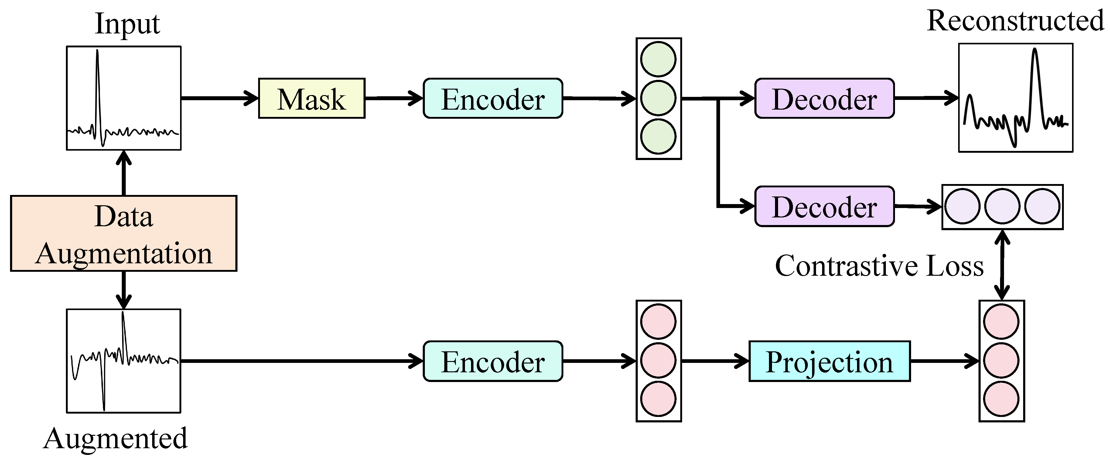
Figure 2.
The risk-oriented contrastive learning representation constraint mechanism generates multi-view representations via risk-equivalent transformations and employs contrastive learning to enhance discrimination and stability across different risk states.
Figure 2.
The risk-oriented contrastive learning representation constraint mechanism generates multi-view representations via risk-equivalent transformations and employs contrastive learning to enhance discrimination and stability across different risk states.
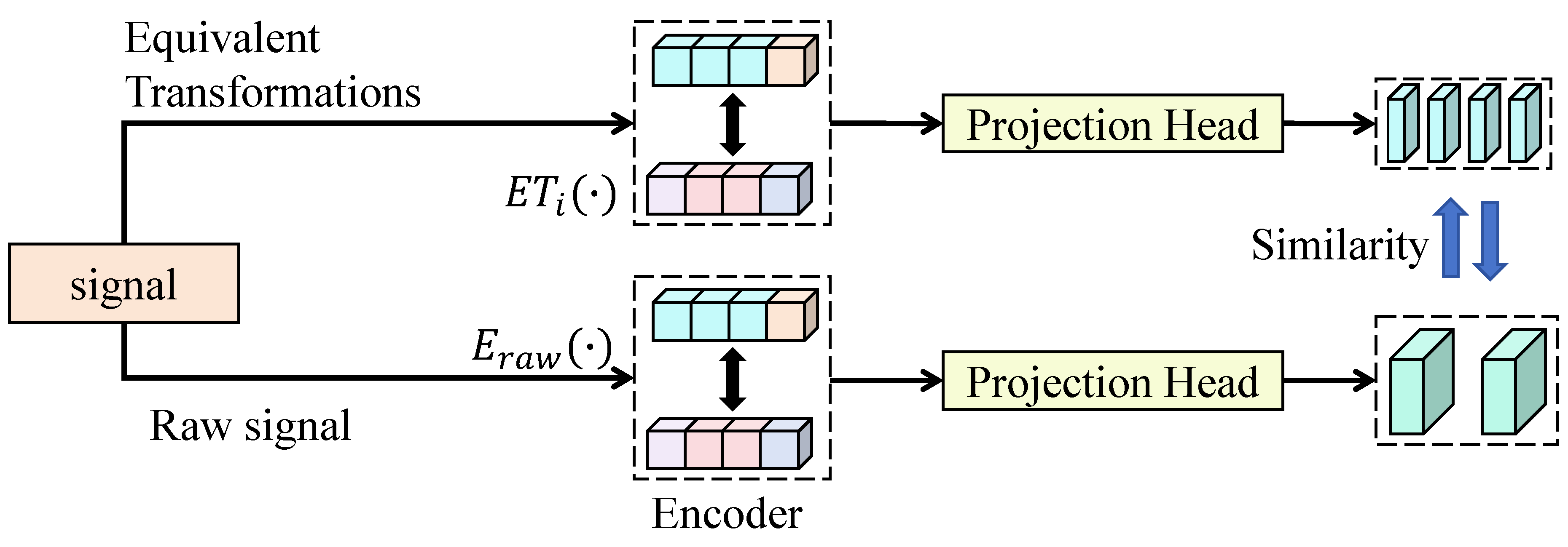
Figure 3.
The risk representation and downstream prediction task alignment strategy aligns learned risk representations with multi-task prediction objectives via learnable transformations and a mixture-of-experts mechanism for adaptive and dynamic decision-making.
Figure 3.
The risk representation and downstream prediction task alignment strategy aligns learned risk representations with multi-task prediction objectives via learnable transformations and a mixture-of-experts mechanism for adaptive and dynamic decision-making.
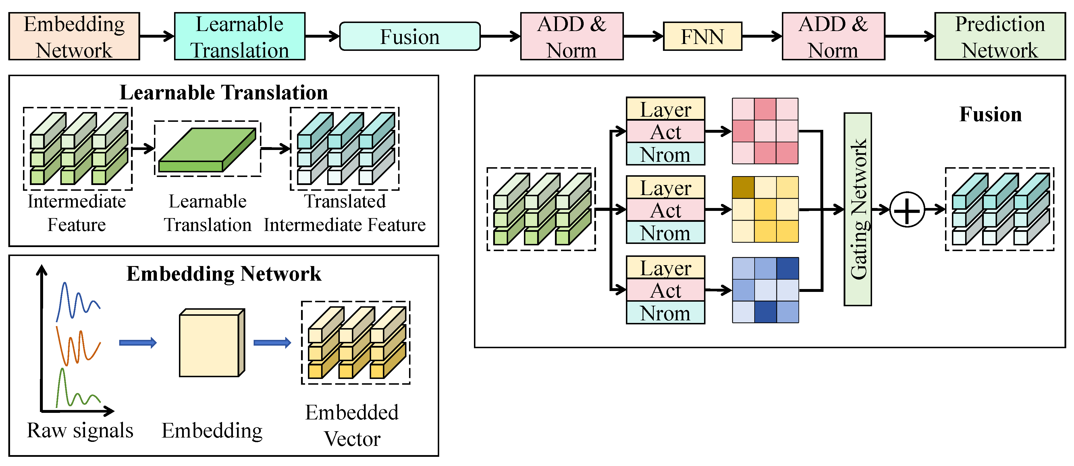
Figure 4.
ROC curve comparison of different models for investment risk classification, where the proposed method achieves the highest AUC and demonstrates superior risk discrimination capability.
Figure 4.
ROC curve comparison of different models for investment risk classification, where the proposed method achieves the highest AUC and demonstrates superior risk discrimination capability.
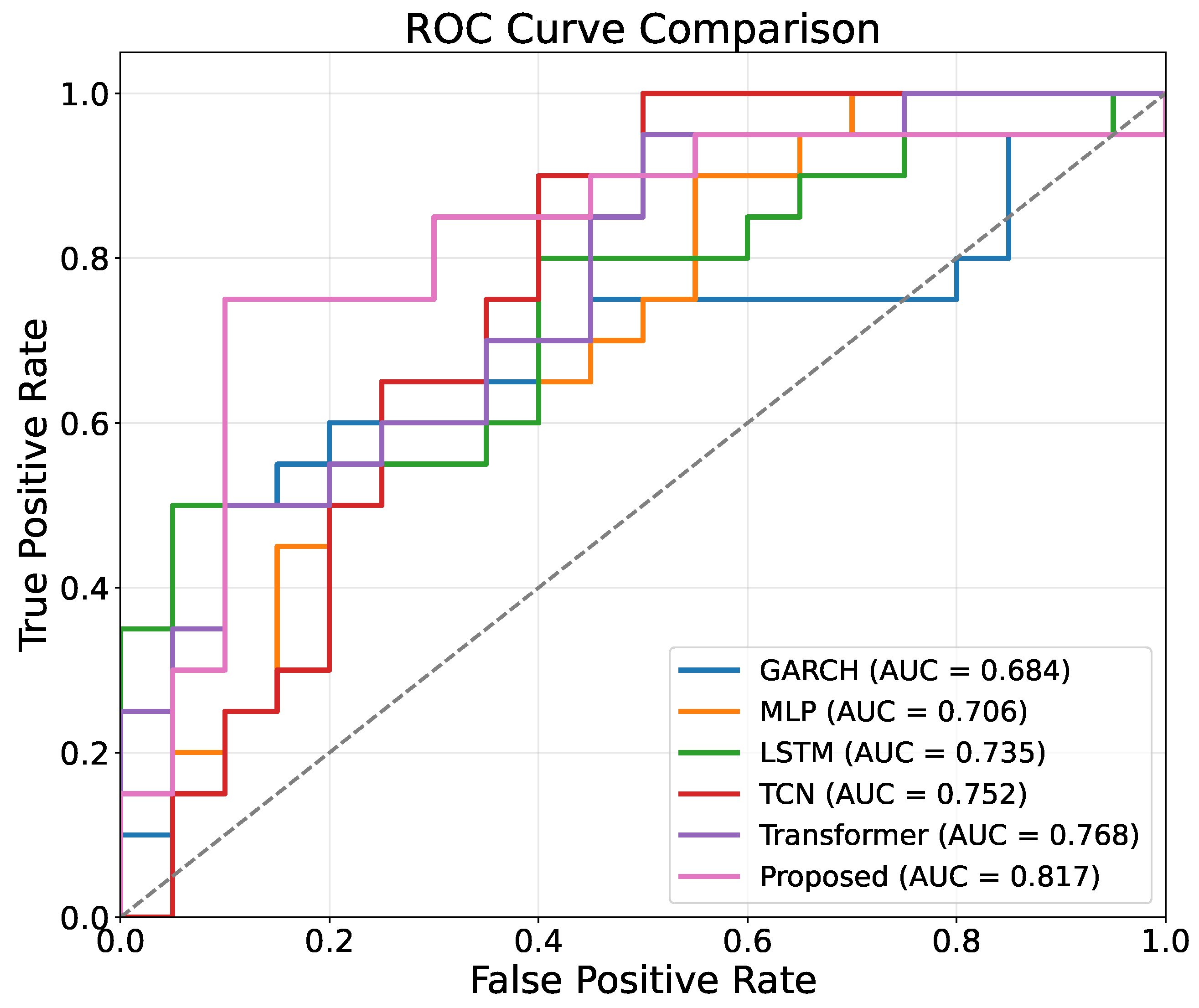
Figure 5.
AUC distribution comparison across different ablation variants, where the full model achieves the highest and most stable risk identification performance.
Figure 5.
AUC distribution comparison across different ablation variants, where the full model achieves the highest and most stable risk identification performance.
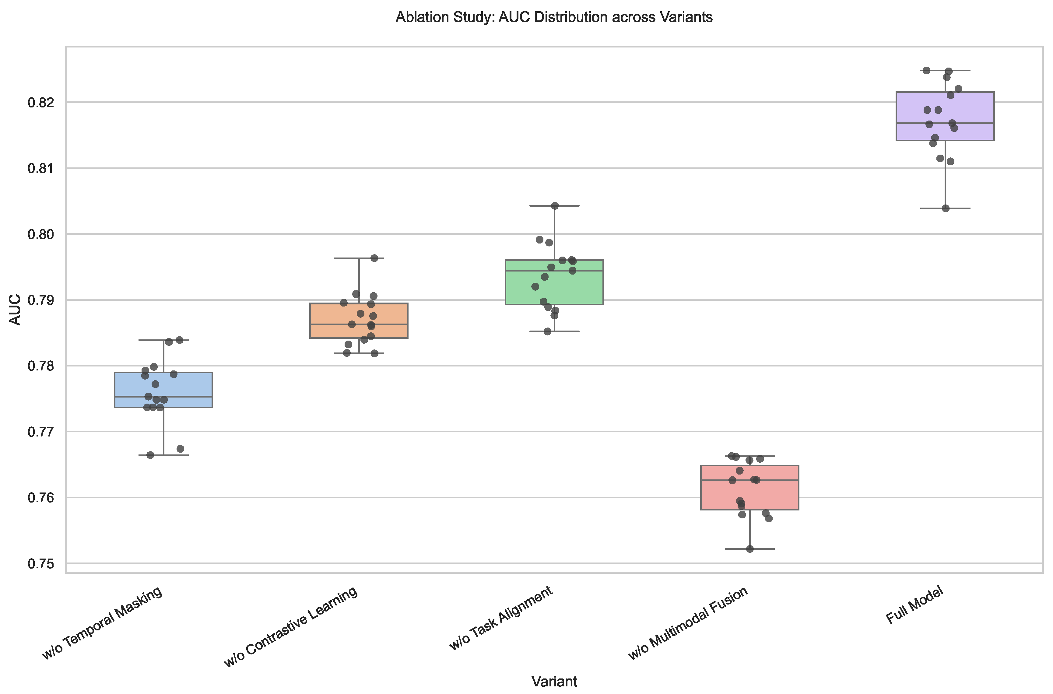
Figure 6.
AUC comparison of LSTM, Transformer, and the proposed method under different market conditions shows that the proposed method achieves the best predictive performance in normal, high-volatility, and extreme-shock markets.
Figure 6.
AUC comparison of LSTM, Transformer, and the proposed method under different market conditions shows that the proposed method achieves the best predictive performance in normal, high-volatility, and extreme-shock markets.
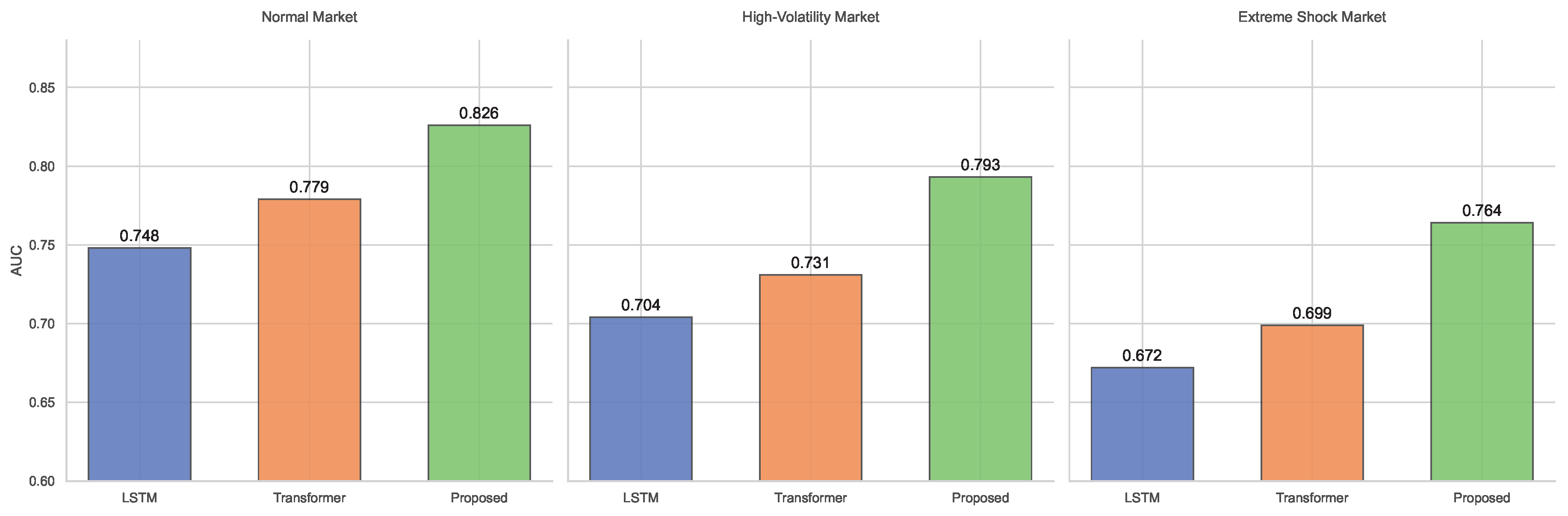

Table 1.
Multi-source hardware sensing financial risk perception dataset composition.
| Data Type | Sensors | Data Volume |
|---|---|---|
| Terminal Interaction | Touch sensors, inertial measurement sensors | 3,850,000 |
| Network Link | Network traffic sensors, link latency sensors | 2,740,000 |
| Device State | Temperature sensors, voltage sensors | 960,000 |
| Order Flow | Order flow intensity sensors, order book depth sensors | 8,750,000 |
| Trading Environment | Environmental temperature and humidity sensors, vibration sensors | 620,000 |
| Clock Synchronization | Clock offset sensors, synchronization error sensors | 410,000 |
| Abnormal Operation | Operation frequency sensors, response latency sensors | 1,180,000 |
Table 2.
Performance comparison of different models on investment risk prediction tasks.
| Method | MSE ↓ | MAE ↓ | RMSE ↓ | IC ↑ | RankIC ↑ | AUC ↑ |
|---|---|---|---|---|---|---|
| GARCH | 0.0287 | 0.1245 | 0.1694 | 0.312 | 0.287 | 0.684 |
| MLP | 0.0259 | 0.1168 | 0.1609 | 0.346 | 0.318 | 0.706 |
| LSTM | 0.0226 | 0.1047 | 0.1503 | 0.392 | 0.361 | 0.735 |
| TCN | 0.0213 | 0.1012 | 0.1459 | 0.415 | 0.386 | 0.752 |
| Transformer | 0.0198 | 0.0965 | 0.1407 | 0.438 | 0.407 | 0.768 |
| Proposed | 0.0164 | 0.0851 | 0.1281 | 0.496 | 0.462 | 0.817 |
Table 3.
Ablation study of the proposed model.
| Variant | MSE ↓ | MAE ↓ | RMSE ↓ | IC ↑ | RankIC ↑ | AUC ↑ |
|---|---|---|---|---|---|---|
| Proposed w/o Temporal Masking Module | 0.0192 | 0.0957 | 0.1386 | 0.447 | 0.416 | 0.776 |
| Proposed w/o Risk-Oriented Contrastive Learning | 0.0185 | 0.0926 | 0.1360 | 0.459 | 0.428 | 0.789 |
| Proposed w/o Task Alignment Strategy | 0.0179 | 0.0908 | 0.1338 | 0.468 | 0.437 | 0.795 |
| Proposed w/o Multimodal Fusion | 0.0204 | 0.0993 | 0.1428 | 0.431 | 0.398 | 0.761 |
| Proposed Full Model | 0.0164 | 0.0851 | 0.1281 | 0.496 | 0.462 | 0.817 |
Table 4.
Robustness comparison under different market conditions.
| Market Condition | Method | MSE ↓ | RMSE ↓ | IC ↑ | AUC ↑ |
|---|---|---|---|---|---|
| Normal Market | LSTM | 0.0205 | 0.1432 | 0.408 | 0.748 |
| Transformer | 0.0181 | 0.1345 | 0.451 | 0.779 | |
| Proposed | 0.0153 | 0.1237 | 0.508 | 0.826 | |
| High-Volatility Market | LSTM | 0.0318 | 0.1783 | 0.347 | 0.704 |
| Transformer | 0.0289 | 0.1700 | 0.382 | 0.731 | |
| Proposed | 0.0227 | 0.1507 | 0.456 | 0.793 | |
| Extreme Shock Market | LSTM | 0.0396 | 0.1990 | 0.301 | 0.672 |
| Transformer | 0.0354 | 0.1881 | 0.336 | 0.699 | |
| Proposed | 0.0275 | 0.1658 | 0.421 | 0.764 |
Table 5.
Model performance changes under different sensor removal settings
| Removed Sensor Type | MSE ↓ | MAE ↓ | RMSE ↓ | IC ↑ | RankIC ↑ | AUC ↑ |
|---|---|---|---|---|---|---|
| Full Model | 0.0164 | 0.0851 | 0.1281 | 0.496 | 0.462 | 0.817 |
| w/o Terminal Interaction Sensors | 0.0181 | 0.0917 | 0.1345 | 0.463 | 0.431 | 0.789 |
| w/o Network Link Sensors | 0.0187 | 0.0932 | 0.1368 | 0.457 | 0.425 | 0.782 |
| w/o Device State Sensors | 0.0175 | 0.0896 | 0.1322 | 0.471 | 0.438 | 0.795 |
| w/o Order Flow Sensors | 0.0201 | 0.0978 | 0.1418 | 0.438 | 0.401 | 0.768 |
| w/o Trading Environment Sensors | 0.0172 | 0.0889 | 0.1311 | 0.474 | 0.441 | 0.798 |
Disclaimer/Publisher’s Note: The statements, opinions and data contained in all publications are solely those of the individual author(s) and contributor(s) and not of MDPI and/or the editor(s). MDPI and/or the editor(s) disclaim responsibility for any injury to people or property resulting from any ideas, methods, instructions or products referred to in the content. |
© 2026 by the authors. Licensee MDPI, Basel, Switzerland. This article is an open access article distributed under the terms and conditions of the Creative Commons Attribution (CC BY) license (http://creativecommons.org/licenses/by/4.0/).
Copyright: This open access article is published under a Creative Commons CC BY 4.0 license, which permit the free download, distribution, and reuse, provided that the author and preprint are cited in any reuse.


