

Submitted:
12 May 2026
Posted:
13 May 2026
You are already at the latest version
Abstract
Transport infrastructure is commonly viewed as a key driver of development, alt-hough its actual contribution remains debated and appears to be dependent on geo-graphical and economic context. This study investigates the impact of transport infra-structure on regional economic growth in Romania, with a particular focus on spatial spillover effects Using panel data for Romanian regions over the period 2000–2024, the analysis applies spatial econometric techniques to capture both direct and indirect ef-fects of transport infrastructure and economic factors. A structured model selection procedure, based on Lagrange Multiplier tests and robust diagnostics, supports the use of the Spatial Autoregressive Model (SAR) as the preferred specification. The results reveal significant spatial dependence in regional economic performance, indicating that growth processes extend across regional boundaries. Nonetheless, the findings show that transport infrastructure does not exert a statistically significant direct effect on economic growth once spatial and structural factors are controlled. Instead, labor and private gross capital formation emerge as the primary drivers, generating both strong local impacts and substantial spillover effects. These results suggest that transport infrastructure acts mainly as an enabling factor rather than a standalone driver of growth, making the concept of “political mythification” of transport infra-structure effectiveness relevant in the Romanian context.
Keywords:
transport infrastructure
; regional economic growth
; spatial autocorrelation
; spillover effects
; SAR model
1. Introduction
Transport infrastructure is widely recognized as a fundamental driver of economic development, shaping the spatial organization of production, trade, and mobility across regions. To promote economic growth, investment in transport infrastructure (both network links and terminals) is a necessary condition along with positive economic externalities (e.g., urbanization/agglomeration, high skilled labor market) and political factors (e.g., sources of finance, level of investment – local, regional, national or international) [1]. By reducing transport costs and improving connectivity, infrastructure investments facilitate the movement of goods, labor, and knowledge, thereby influencing regional productivity and growth [2,3,4,5,6,7,8,9]. However, these effects are not limited within administrative boundaries. Instead, they extend across space through spatial spillovers, generating interdependencies between regions and contributing to uneven development patterns [10].
Within the European Union, addressing regional disparities has been a long-standing policy objective, supported by substantial investments in transport infrastructure through cohesion policy and trans-European networks. While some regions benefit from high levels of connectivity, diversified economies, and strong integration into trans-European networks, others continue to face structural constraints, limited accessibility and weaker economic performance, particularly in Central and Eastern European countries [11,12,13,14]. European cohesion policy has long emphasized the role of transport infrastructure in reducing these imbalances, aiming to improve territorial integration and promote more balanced development. The extent to which infrastructure investments effectively reduce disparities depends on how their benefits are distributed across space and whether they extend beyond the regions in which they are implemented [14]. Despite these efforts, significant differences in accessibility and economic performance persist. Romania represents a relevant case in this context, characterized by pronounced regional disparities, uneven infrastructure development, and varying degrees of integration into European transport corridors. In Romania, regional disparities are particularly pronounced, reflecting differences in economic structure, investment levels, and connectivity. Although substantial investments in transport infrastructure in recent decades, disparities in both accessibility and economic performance persist. This raises important questions regarding the effectiveness of infrastructure policies in promoting balanced regional development and the extent to which benefits spread across regional boundaries.
This study explores the direct and spatial spillover effects of transport infrastructure on regional economic growth in Romania. The paper provides empirical evidence on how infrastructure investments shape regional development patterns in an emerging European economy. Two research hypotheses are formulated:
H1
(Direct effect): Transport infrastructure has a positive and statistically significant direct effect on regional economic growth in Romania. Regions with higher infrastructure endowment exhibit higher growth rates.
H2
(Spatial spillover effect): Transport infrastructure generates positive and statistically significant spatial spillover effects on economic growth in neighboring regions. Infrastructure improvements in one region increase growth in adjacent regions.
H3
(Disparities effect): Spatial spillover effects contribute to reducing regional disparities in economic growth. Spillovers are relatively stronger in less-developed or lower-accessibility regions, indicating convergence dynamics.
Beyond the national context, the findings have broader implications for understanding infrastructure-leading development in a global perspective. It has been shown that the variation in results is not only attributed to methodological limitations or differences but also reflects the influence of distinct geographical factors [15,16,17]. The results contribute to the growing literature on spatial economic interactions and offer insights relevant for policymakers seeking to enhance the effectiveness of infrastructure investments in promoting balanced regional growth.
The remainder of the paper is structured as follows. Section two reviews the relevant literature on transport infrastructure effects on regional development. This is followed by a description of the study area, data and methodology, including the specification of spatial econometric models. Section four thoroughly details the results. Next, the empirical results are subsequently discussed in relation to econometric models, key growth drivers, and both direct and spillover effects in Romania. Policy implications and directions for future research are outlined. The last section draws the main conclusions of the study.
2. Literature Review
Many studies have reported strong positive effects of transport infrastructure (roads, railways, airports, and ports) on economic growth, while other research has highlighted negative or weak effects, as well as substantial heterogeneity across regions and over time.
Empirical findings indicate that improvements in transport infrastructure have a statistically significant positive effect on local Chinese economic growth [18]. Across models employing different spatial weight matrices, only the specification based on population density reveals negative spillover effects. This outcome can be explained by the high mobility of the population: enhanced transport connectivity facilitates migration from less developed areas toward more prosperous regions. While infrastructure investments stimulate growth in developed areas, they may also hinder economic progress in less developed regions. Hong et al. [6] found that various modes of infrastructure contributed to economic performance differently across Chinese regions. Land transport infrastructure has the greatest impact on economic development, followed by water transport and airway transport infrastructure. Regional disparities persist, and insufficient transport infrastructure is responsible to the slower economic development of Western and Central China. In the same way, the economic impact of the Chinese high-speed rail development varies considerably across cities, showing clear disparities [19]. It tends to generate strong positive effects in economically advanced cities, while having negative or negligible impacts in less developed or declining regions. The high-speed rail can reinforce existing regional inequalities through both growth-enhancing and drain off effects. Equally, the expressway connections do not affect all regions in the same way [20]. While richer areas tend to benefit, poorer counties often rely on more polluting technologies and see higher levels of emissions. The results of Wang et al. [21] indicate that logistics infrastructure is an important driver of economic development in China, with maritime transport playing a significant role in supporting trade and growth. Still, no clear link is found between air transport infrastructure and economic growth, although China turns toward high-tech industries, where air transport may become increasingly important. Kim et al. [22] reveals that once the highways become operational, their influence on economic growth (GDP expansion) and exports is clearly positive. Improved infrastructure boosts production capacity and enhances price competitiveness, which in turn contributes to increased export growth. Also, the enhancement of the accessibility contributed to the improvement of regional economic equity in Korea. A bi-directional causality between economic growth and infrastructure investment was also observed in Central Asia (Armenia, Georgia, Turkey) [23].
The study of Saidi et al. [24] focusing on MENA (the Middle East and North Africa) countries showed that transport infrastructure positively contributes to economic growth in all regions by decreasing congestion, promoting the use of energy-efficient transport modes and alternative technologies, increasing the attractiveness of regions and therefore encouraging foreign direct investment inflows. The Belt and Road initiative in Eastern Africa promotes trade and economic growth through transport infrastructure development [25].
An analysis for EU-28 countries showed that transport infrastructure has a significant and positive impact on economic growth, with a clear long-run causal relationship between the two [26]. This relationship is improved by the quality of public sector performance, being more effective when supported by strong institutions and sound policies. Similarly, Gherghina et al. [27] observed a clear positive relationship between investment in road transport infrastructure and economic growth. Spending on road infrastructure generates direct employment, attracts investors, and enhances firms’ productivity. The impact of high-speed rail on economic growth varies depending on the level of regional development and local conditions [28]. More developed regions experience greater convergence and growth effects, while less developed regions may see more limited or uneven gains. The effectiveness in promoting economic growth depends on connectivity with local networks. In the UK, the impact of transport infrastructure on economic growth is not uniform over time [29]. Over the long term, expanding transport infrastructure has a clear and positive effect on economic growth, whereas in the short term the impact can be negative. Raising the connectivity of the transportation network and increasing the number and density of network nodes are solutions to support a better regional economic integration. Transport infrastructure in Croatia, particularly road network improvements, has a heterogeneous impact on local development, showing positive effects in the hinterland but statistically insignificant impacts on the coastline [30]. Positive effects of the investments in transport infrastructure are reported for Spain [3,31], Germany, France, Italy [32], Greece [33], Poland [34], Latvia [35], Switzerland [36]. The results suggest that there is a clear link between the development of major cities and higher-level infrastructure, while this relationship is much weaker at the broader regional level. At the same time, the findings indicate that large-scale infrastructure investments tend to have the strongest impact during the early stages of economic development, with their influence diminishing as regions become more advanced [34,37,38].
Other research has highlighted negative or weak effects, as well as substantial heterogeneity across regions and over time. Deng [39] considered that the validity and significance of transport capacity as a driver of productivity and economic growth remain uncertain and questionable. The connectivity characteristic of transport infrastructure enables spillover effects that may either enhance or hinder productivity and economic growth in neighboring regions. Accordingly, the purported economic benefits of transport infrastructure investment in one region may entail costs borne by others. In the absence of interregional coordination, a level of investment that appears appropriate for a specific region may generate adverse consequences for neighboring competing areas. Chen et al. [40] revealed that transportation infrastructure inequality plays a dual and evolving role in economic development. While it may initially support growth by fostering agglomeration, it ultimately contributes to unbalanced development across national and regional scales and can become a structural bottleneck that hinder overall performance. Proximity to large urban areas tends to yield either higher output or lower costs, yet empirical results vary considerably. This suggests that outcomes are contingent upon geographic specificities and methodological choices [5,41]. Also, polarization effects dominate the early phase, giving way to diffusion effects as maturity is reached [42]. Konno et al. [10] demonstrated that road infrastructure has an inverse correlation with regional productivity, spillover effects are directly positive, while the net effect is positive but insignificant. Sometimes the economic development cannot be attributed solely to transport infrastructure or its contribution is insignificant [43,44]. Li et al. [45] found that the urban–industrial land use efficiency system and accessibility of the highway networks system were not mutually improved. Rietveld [15] concluded that is a limited impact of transport infrastructure on spatial economic development. Transport infrastructure, by itself, does not appear to have a significant impact on regional economic growth in Europe, especially once a basic level of infrastructure is already achieved [37]. This suggests that relying on infrastructure investment as the main driver of growth may not be as effective as often assumed. Instead, other factors play a much more important role, particularly increasing accessibility, agglomeration and proximity, investment in research and development, the ability to absorb innovation, employment, and migration [1,38,46,47]. These elements contribute directly to productivity and long-term economic performance. The findings also raise concerns about how resources are allocated. There is strong political interest in the economic impact of transport infrastructure investments. Business groups, companies’ associations, as well as regional authorities, often assume that these investments bring substantial economic benefits. In this respect, Offner [48] use the term of “political mythification”.
3. Methodology
3.1. The Study Area
Romania, located in Eastern Europe and a member of the European Union since 2007, provides a relevant case for examining the relationship between transport infrastructure and regional economic development (NUTS 2). The country is divided into eight development regions (North-West, Center, North-East, South-East, South, Bucharest–Ilfov, South-West, and West) created under the EU’s cohesion framework (Figure 1).
These regions display significant disparities in terms of economic performance, infrastructure endowment, and accessibility [49,50]. From an economic perspective, Romania has experienced sustained growth over the past two decades but unevenly distributed. The Bucharest–Ilfov region stands out as the main economic hub, concentrating a large share of GDP, foreign direct investment, and high-value services. Also the West and North-West regions experienced dynamic economic evolution. In contrast, regions such as North-East and South-West lag behind, facing structural challenges including lower productivity, weaker connectivity, and limited investment attractiveness [51,52,53]. Recent articles investigating Romania’s regional development [54,55] provided a multidimensional approach to regional polarization and unequal development, emphasizing the eminent role of large urban growth poles.
Transport infrastructure development in Romania has been a central component of national and European policy agendas, particularly through EU Cohesion and Structural Funds. The country’s transport network includes road, rail, air, and inland waterway systems, with roads—especially highways—playing a dominant role in recent investments. Despite progress, Romania still faces notable infrastructure gaps compared to other EU member states, particularly in terms of motorway density and quality of rail services [51,56]. Western regions benefit from better connections to Central European markets, while eastern and southern regions remain relatively peripheral. This uneven accessibility influences regional economic dynamics, as improved connectivity tends to facilitate trade, labor mobility, and investment flows. In this context, transport infrastructure is considered a key factor shaping regional growth patterns in Romania. Romania represents a compelling study area for analyzing how transport infrastructure development interacts with regional economic growth, highlighting both its potential benefits and its limitations in addressing territorial inequalities.
3.2. Variables
The analysis is based on a panel dataset covering Romania’s development regions over the years 2000–2024, using data provided by the National Institute of Statistics. The selected variables are intended to reflect the main economic, social, and spatial factors that influence regional growth (Table 1).
GDP per capita is used as the primary indicator of economic performance, as it effectively captures differences between regions and provides a consistent basis for comparison [6,57]. The main explanatory variables capturing the development of transport infrastructure are road, highway and railway network density. These indicators reflect the spatial intensity of transport networks and their capacity to support economic activity, market size, accessibility and regional connectivity [6,26,30,34,37,39,57]. In selecting control variables, we incorporated private gross fixed capital formation, labor force, research and development expenditure, and urbanization rate. These factors are widely recognized in the literature as key drivers of economic growth and help ensure that the model captures the main influences beyond transport infrastructure. Private gross fixed capital formation is an important driver of economic growth, as it reflects private sector investment in assets such as machinery, buildings, and software. These investments signal business confidence, while also supporting higher production capacity, innovation, and job creation over time [3,18,26,29]. Labor force levels are fundamental drivers of production capacity [3,18,26,57], while R&D intensity is crucial for long-term economic vitality [37,57]. Urbanization affects labor allocation, concentrates markets, services, reduces the cost of doing business, trading goods, and accessing information, and through agglomeration effect it might drain resources from neighboring zones [28,29,38,57]. All variables are expressed in the model in logarithmic form to reduce skewness and heteroskedasticity and to allow for elasticity-based interpretation, while ratio variables such as urbanization are kept in levels.
3.3. Spatial Autocorrelation Test
The global Moran’s I index is used to assess the presence of spatial dependence in regional economic performance. It evaluates whether the observed spatial distribution of GDPPC is characterized by clustering, dispersion, or randomness by comparing values across neighboring NUTS 2. A positive value of Moran’s I indicates positive spatial autocorrelation, thus regions with similar levels of economic performance tend to group into spatial clusters. A negative value suggests spatial dispersion, where rich regions alternate with poor ones. A value close to zero implies a random spatial pattern with no significant spatial structure.
The Moran’s I index for year () is computed as follows:
where
is the value of the variable of interest (GDP per capita) in region at time ,
represents the mean value of GDP per capita across all regions in year ,
is the number of regions,
represents the spatial weight between regions and .
The spatial weights matrix captures the structure of spatial interactions between NUTS 2. To investigate the spatial autocorrelation, two forms of the spatial matrix are used: (i) a rook-contiguity matrix and (ii) a distance-based matrix using k-nearest neighbors (k = 3). The first specification is based on rook contiguity, where two regions are considered neighbors if they share a common border:
This approach is in line with Tobler’s first law of geography, reflecting the idea that spatial autocorrelation is more likely to occur between regions with direct physical adjacency.
The second approach uses a k-nearest neighbors (KNN) matrix. Under this assumption, each NUTS 2 is connected to its three closest neighboring regions based on geographical distance between regional centroids. The spatial weights are defined as:
In both cases, the spatial weights matrix is row-standardized (). This transformation allows comparability across regions with different numbers of neighbors.
3.4. Econometric Models Specification
The baseline econometric specification is given by the Ordinary Least Squares (OLS) model:
where:
- is the dependent variable;
- – the regressor variables (ln(ROADD), ln(HWAYD) etc.);
- - the model coefficients;
- - the error;
- – the region number;
- the time period (year);
- – the regressor number.
The coefficients quantify the influence of the regressors on the dependent variable. The pooled OLS model assumes homogeneity across regions and ignores unobserved effects, which may lead to biased estimates. To control for unobserved time-invariant heterogeneity across regions, the fixed effects model is specified as:
where captures time invariant region-specific effects, such as geography or historical determinants.
Regional economies are also subject to specific events over time (e.g., macroeconomic crises or national policies). Therefore, a two-way fixed effects controls for both regional and temporal heterogeneity:
where represents time-specific effects such as nationwide policy changes, economic conditions or geopolitical events.
The selection between fixed and random effects is evaluated using the Hausman test [58]. Before estimating spatial econometric models, the presence of spatial dependence is assessed using both global and local diagnostic tests. Global spatial autocorrelation is evaluated using the Moran’s I statistic. In addition, Lagrange Multiplier (LM) tests are applied to detect spatial dependence in the error term [59].
Spatial regression models allows us to uncover relationships between economic variables by accounting not only for their direct interactions, but also for the way they influence each other across NUTS 2.
The first investigated spatial model is the Spatial Autoregressive Model (SAR):
where:
- are the elements of the spatial weight matrix W;
- is the parameter that quantifies spatial dependence.
The model assumes that GDPPC in a given region depends not only on its own economic characteristics (the explanatory variables ), but also on the GDPPC levels of neighboring regions, weighted by the spatial weight matrix . This matrix reflects the considered spatial structure (rook-contiguity or KNN). The parameter measures the strength of spatial dependence:
- if , there are positive spillovers (advanced regions positively influence their neighbors);
- if , negative spatial dependence arises (spatial divergence);
- if , the model reduces to a standard regression without spatial effects.
The coefficients capture the direct effects of the explanatory variables on . The SAR model also generates indirect (spillover) effects, since changes in one region propagate through the spatial network.
The second instance, Spatial Error Model (SEM), considers that the dependence is manifested in the error terms, not in the dependent variable as in SAR, suggesting that there are unobserved factors with a spatial structure influencing the outcome:
Equation (8) is a standard regression form, while Equation (9) shows that the error term is spatially autocorrelated. is the white noise (independent and identical distributed). The parameter points out the strength and direction of spatial dependence in the error term:
- if , there is positive spatial correlation in the errors (similar shocks across adjacent regions);
- if , negative spatial correlation;
- if , no spatial dependence and the model reduces to ordinary regression.
The third model is the Spatial Durbin Model (SDM) that incorporates spatial dependence in both the dependent variable and the explanatory variables:
SDM combines three key components:
- spatial lag of the dependent variable , capturing how outcomes in neighboring regions affect region , where measures the strength of spatial dependence (similar to SAR);
- the standard regressors , where coefficients reveal direct effects of local explanatory variables;
- spatial lags of the explanatory variables , with coefficients getting the spillover effects from neighboring regions’ characteristics.
If , the model reduces to the SAR model, and if , it becomes a model with only spatially lagged regressors.
The selection among the spatial regression models follows a structured econometric procedure. Firstly, the Lagrange Multiplier (LM) tests detect the presence of spatial dependence in data. When both spatial lag and spatial error dependence are indicated, the analysis proceeds with the estimation of the more general SDM specification, which encompasses both SAR and SEM as special cases. To determine whether the SDM can be simplified, a Wald test [59] is employed to assess the joint significance of the coefficients associated with the spatially lagged explanatory variables. This test evaluates whether the SDM can be reduced to a more parsimonious specification.
4. Results
4.1. Data Descriptive Analysis
Table 2 exhibits the descriptive statistics of the variables used in the analysis.
Regional GDP per capita (GDPPC) exhibits an average value of 8014 EUR, with a large standard deviation, reflecting pronounced regional disparities. The strong positive skewness (2.71) indicates that a small number of regions (Bucharest-Ilfov, West and North-West), register significantly higher income levels compared to the rest. Transport infrastructure variables also display considerable heterogeneity. Road density (ROADD) shows a high dispersion, suggesting uneven development of road networks across regions. Highway density (HWAYD) is particularly skewed (3.10), with many regions having very low or zero values in earlier years (North-East, South-West), while a few regions experienced substantial expansion. Similarly, rail density (RAILD) presents notable variation, although less extreme than highways, indicating differences in legacy infrastructure across regions. Economic control variables further highlight structural disparities. Private gross fixed capital formation (PCAPIT) shows a high degree of variability (skewness = 3.45), suggesting that investment is concentrated in a limited number of regions. Research and development expenditure (R&D) is the most unevenly distributed variable, with very high skewness (4.23), indicating that innovation activities are heavily concentrated in a few economically advanced regions (Bucharest-Ilfov, North-West). In contrast, the labor variable (LABOR) exhibits relatively low dispersion and flat skewness, denoting a more balanced distribution of employment across regions. The urbanization rate (URB) has moderate variation and slight positive skewness, reflecting differences in the degree of urban concentration. The descriptive statistics point to significant regional inequalities across regions of Romania.
4.2. Global Moran’s I Index
The Moran’s I index for both rook contiguity and k-nearest neighbors (k = 3) reveals a consistent pattern over the entire study period (Figure 2).
For the rook-based matrix, the Moran’s I values are slightly negative in all years. None of the associated p-values indicate statistical significance. Therefore, there is no clear evidence that regions with similar levels of economic performance are systematically clustered together, nor that regions with different performance are strongly dispersed. A similar conclusion occurs from the KNN specification, although the Moran’s I values are rather more negative. All the p-values are above conventional significance thresholds. The results from both weighting schemes shows that the spatial pattern appears largely random.
4.3. Collinearity, Variable Selection and Ordinary Regression Testing
Due to the potential overlap between the regional development driving variables, the multicollinearity is assessed using the Variance Inflation Factor (VIF). To ensure a robust evaluation, VIF values are computed using pooled data across all regions and years, capturing the overall correlation structure of the explanatory variables within the panel (Table 3).
The results indicate substantial multicollinearity among variables, especially those related to infrastructure (road, rail, and highway density) and expenditures and social activity (capital formation, R&D expenditures, and urbanization). This suggests that they carry overlapping information and keeping all of them may compromise the stability of the models. To address this issue, variables are retained or excluded based on two criteria: (i) statistical evidence of multicollinearity (a VIF < 10 is recommended) and (ii) economic evidence and theoretical representativity. Within the infrastructure group, highway density is selected because its VIF is 4.59 and it captures direct effects through reduced transport costs and improved mobility of goods and people across national and international territory and represents the backbone for connecting to the European TEN-T network. The highways construction has been accelerated over the past years in regions with feeble investments (North-East, South-West) and also in the perspective of EU ascension of Moldova and Ukraine to provide their connection to the European network. The road density has a VIF at the limit of the threshold. The variable is preserved in the condensed model due to its role in supporting the highest share of cargo flows movement both for domestic and international trade. Within the group of economic and social controls, private gross fixed capital formation is retained as the key variable capturing extensive and intensive technological development allowing economic scalability, jobs creation and labor migration. Labor is maintained in the final specification, as it exhibits low multicollinearity and represents a fundamental production factor. As a result, the final model specification includes road and highway density, private gross fixed capital formation, and labor as the core explanatory variables. This parsimonious specification ensures stable estimation, avoids redundancy, and preserves the economic interpretability of the model.
The selection between fixed and random effects is assessed using the Hausman test. The Hausman test strongly rejects the null hypothesis of no systematic difference between the fixed and random effects estimators (χ² = 459.67, p < 0.001). The results indicate that the fixed effects specification is preferred, suggesting that unobserved regional heterogeneity (e.g., geographic position, historical development, regional investment policy) is correlated with the explanatory variables (infrastructure, labor , and R&D expenditure). The Romanian regions’ evolution is not random, as consequence their intrinsic structural characteristics are meaningful. Therefore, the fixed effects specification is preferred.
For the reduced model, Table 4 reports the results obtained from three model specifications: pooled OLS, fixed effects, and two-way fixed effects.
The comparison highlights how controlling for unobserved heterogeneity substantially changes both the magnitude and the interpretation of the coefficients.
In the baseline OLS model, all variables are highly statistically significant, and the model exhibits a high explanatory power (Adjusted R² = 0.952). Road and highway density, and private gross capital formation have positive significant effects. The negative sign for labor is driven by general decrease in population and employment due to emigration and reduced birth-rate.
The presence of regional fixed effects alters the results considerably. Road density becomes positive and strongly significant, suggesting that, within regions, improvements in road infrastructure are associated with higher economic performance. Private capital formation (PCAPIT) remains positive and highly significant, confirming its role as a key driver of growth. Labor continues to display a negative coefficient, indicating time-invariant regional characteristics in employment process. Highway density remains weakly negative, with only marginal statistical significance.
The two-way fixed effects model controls for both regional and time-specific heterogeneity. In this specification, the coefficient of labor becomes positive and highly significant. This shift indicates that increases in employment within a region contribute positively to economic growth once structural differences and common time effects are taken into account. Private gross capital formation remains positive and statistically significant, although its magnitude decreases, suggesting that part of its effect is absorbed by time and regional fixed effects. In contrast, both road density and highway density lose statistical significance in the two-way fixed effects model. This suggests that the direct impact of transport infrastructure on regional GDP per capita is limited when broader structural and temporal dynamics are considered. The earlier significance observed in OLS and fixed effects models appears to reflect cross-sectional differences rather than true causal effects.
The results indicate that regional economic growth is primarily driven by capital accumulation and labor dynamics, while the direct contribution of transport infrastructure is less clear.
The Lagrange Multiplier (LM) test is employed to detect the existence of spatial interdependence in the panel data (Table 5).
The Lagrange Multiplier test statistic is statistically significant at the 5% level for the rook-contiguity model, indicating the presence of spatial dependence in the data. In contrast, for KNN weight matrix the spatial effects are weak. These findings support the further inclusion of spatial effects in the econometric specification for rook-contiguity.
4.4. Spatial Econometric Models and Spillover Effects
Three econometric models are analyzed to investigating the spatial effects: Spatial Autoregressive (SAR), Spatial Error (SER), and Spatial Durbin Model (SDM). The selection of the appropriate model is based on a comprehensive set of diagnosis tests: Lagrange Multiplier for lags and errors, robust LM, and Wald tests (Table 6).
Both the LM test for spatial lag dependence and the LM test for spatial error dependence are highly significant (p < 0.001). These results prove that regions’ GDP per capita are spatially correlated. Since standard LM tests cannot clearly distinguish between alternative spatial processes, locally robust versions of these tests are considered. The robust LM test for spatial lag dependence remains highly significant (LM = 18.024, p < 0.001), indicating that spatial dependence in the GDPPC persists even after controlling for potential spatial error effects. In contrast, the robust LM test for spatial error dependence is moderately significant (LM = 5.1015, p = 0.024), suggesting that spatial error dependence exists but plays a secondary role. These findings reveal that spatial correlation is primarily driven by lag effects (SAR), reflecting genuine interactions between neighboring regions, while error dependence (SEM) is comparatively weaker and likely reflects unobserved common factors.
To determine if the Spatial Durbin Model (SDM) provides additional explanatory power over the Spatial Autoregressive (SAR) model, the Wald test is employed to assess the joint significance of the spatially lagged explanatory variables. The null hypothesis states that the coefficients associated with these variables are equal to zero. The results of the Wald test indicate that the null hypothesis cannot be rejected (p-value = 0.837), suggesting that the spatially lagged explanatory variables do not contribute significantly to the model. Consequently, the more parsimonious SAR model is retained as the preferred specification. This choice ensures model stability and interpretability while adequately capturing the spatial dependence structure in regional economic growth.
The estimated results of the SAR model are reported in Table 7. The model accounts for both regional heterogeneity and common time effects, while explicitly capturing spatial dependence.
The spatial autoregressive coefficient (λ = 0.185) is positive and statistically significant (p = 0.012), indicating the presence of moderate spatial dependence across regions. This result suggests that regional economic performance is interconnected, as increases in GDPPC in one region are associated with improvements in neighboring regions. The magnitude of λ points to meaningful, yet not excessive, spillover effects.
LABOR emerges as the most important explanatory variable of regional economic growth. The coefficient is positive and highly statistically significant (p < 0.001), indicating that increases in employment are strongly associated with higher GDP per capita. The estimated coefficient (0.496) suggests a substantial elasticity, confirming the central role of labor in driving regional economic performance. Private gross capital formation exhibits a positive and statistically significant effect (p = 0.013). In contrast, the infrastructure variables do not display statistically significant effects. Road density has a positive but insignificant coefficient, while highway density shows a closed to zero value and statistically insignificant effect. Thus, transport infrastructure does not exert a measurable direct impact on regional GDPPC once the spatial dependence is considered.
Figure 3 reports the decomposition of the spatial effects derived from the SAR model, including direct, indirect (spillover), and total effects.
LABOR is by far the main driver of regional economic growth. The direct effect is large and positive (0.501), showing that increases in employment substantially enhance economic performance within the same region. In addition, the indirect effect is also considerable (0.107), indicating that improvements in labor conditions generate significant spillovers to neighboring regions. The total effect (0.608) confirms that labor plays a dominant role not only locally but also in shaping regional dynamics through spatial diffusion. PCAPIT also exhibits positive although smaller effects. The direct effect (0.097) suggests that investment contributes to local economic growth, while the indirect effect (0.021) reflects modest spillover effects. The impact of infrastructure variables is relatively limited. ROADD has a small positive direct effect (0.047) and a weak indirect effect (0.010), its contribution being marginally to regional economic growth. HWAYD does not exhibit a significant effect. Both the direct and indirect effects are close to zero, with a negligible total effect. The highway infrastructure does not generate measurable economic benefits within the SAR model.
5. Discussion
The findings of this study offer a perspective on the determinants of regional economic growth and the role of spatial interactions in Romania. By relating ordinary regression and spatial econometric models, the analysis provides evidence on both direct and indirect mechanisms through which growth is generated and especially the role of the transport infrastructure.
5.1. Model Selection
From a methodological perspective, the study demonstrates the importance of appropriate model selection in spatial econometrics. The baseline models were estimated using OLS and fixed effects specifications. The Hausman test strongly rejected the null hypothesis of no systematic differences between fixed and random effects, indicating that the fixed effects model is preferred. The presence of spatial dependence under rook-contiguity weight matrix was assessed using Moran’s I and Lagrange Multiplier (LM) tests. Both standard and robust LM tests indicated significant spatial dependence, with stronger evidence for spatial lag dependence (SAR) relative to spatial error dependence (SEM). These results justify the inclusion of spatial effects in the econometric specification. The spatial econometric models were estimated, including the Spatial Autoregressive (SAR) model and the more general Spatial Durbin Model (SDM). To determine the appropriate specification, a Wald test was employed to assess the joint significance of the spatially lagged explanatory variables. The results indicate that the additional SDM terms do not significantly improve the model. Based on these results, the SAR model is retained as the preferred specification. This choice reflects the principle of parsimony, as the simpler model adequately captures the spatial dependence structure.
5.2. Economic Growth Drivers
Although a number of seven explanatory variables were initially considered, the variance inflation factors suggested strong autocorrelation amid them. Subsequently, a reduced panel considering only four variables (road and highway density, labor and private gross capital formation) was adopted.
A consistent result across all estimated specifications is the strong and positive impact of LABOR on regional economic performance. In the SAR model, labor emerges as the dominant determinant of growth, exhibiting both a large direct effect and substantial spillover effects across neighboring regions. This indicates that improvements in employment not only enhance local economic outcomes but also generate significant interregional benefits. The robustness and magnitude of this effect suggest that labor dynamics represent the primary channel through which regional economies expand and interact. Several mechanisms can explain this pattern. Higher employment increases local income and consumption, which stimulates consumption of goods and services both within the region and in neighboring areas through trade. Labor mobility facilitates the diffusion of skills and knowledge across regions, allowing productivity gains to spread spatially [60]. Studies at European level shows that regional growth is strongly linked to labor market conditions and human capital, with spillover effects playing a key role in shaping spatial development patterns [37,61].
Private gross capital formation also plays an important, though more moderate role in all models. The results show a positive and statistically significant effect of PCAPIT on GDP per capita, both locally and through spatial spillovers. This finding is consistent with previous studies, where capital accumulation contributes to productivity and income generation [3,18,26,29,46].
In contrast, the role of transport infrastructure appears limited and less direct. The empirical results indicate that both road density and highway infrastructure do not exert statistically significant effects on regional economic growth once fixed effects and spatial dependence are considered. This suggests that infrastructure investments do not automatically translate into immediate or measurable gains in local economic performance. The results are in line with the recent evidence indicating that the economic impact of infrastructure is strongly influenced by regional context and conditions [8]. Similar insignificant direct and spillover effects of transport infrastructure on regional growth were reported in literature [15,37,43,44].
5.3. Research Hypothesis Testing
This study evaluates three hypotheses concerning the role of transport infrastructure and spatial spillovers in regional economic growth.
- H1 (direct effects of infrastructure) is not supported. Once two-way fixed effects and spatial dependence are accounted for, transport infrastructure variables do not exhibit statistically significant effects on GDPPC. This suggests that transport infrastructure alone does not constitute a primary driver of regional growth in the Romanian context.
- H2 (existence of spatial spillovers) is supported. The positive and significant spatial autoregressive coefficient confirms that regional economies are interdependent. However, the decomposition of effects indicates that these spillovers are driven predominantly by economic factors (LABOR and PCAPIT), rather than by transport infrastructure (ROADD and HWAYD). This points to a diffusion mechanism based on economic activity rather than physical connectivity alone.
- H3 (spillovers reduce regional disparities) receives limited support. Although spatial dependence is present, its sources do not indicate a convergence process driven by transport infrastructure. Instead, spillovers appear to reinforce existing economic structures, suggesting that transport infrastructure dynamic does not automatically translate into balanced regional development.
The presence of a significant spatial autoregressive coefficient (λ = 0.185) advocates that regional economies are interconnected and the growth processes extend beyond NUTS 2 boundaries. In this context, transport infrastructure may play an indirect role by facilitating persons and commodities mobility, reducing transport costs, and supporting interregional interactions, even if these effects are not directly captured in the estimated coefficients. Therefore, rather than acting as a primary driver of economic growth, transport infrastructure acts more as an enabling condition that supports spatial economic integration.
5.4. Policy Implications
The results outline several important policy implications, reflecting the dominant role of economic variables and the limited contribution of transport infrastructure. First, the strong and consistent impact of labor highlights the importance of employment policies and human capital development. Policies aimed at improving labor market participation, workforce skills, and mobility are likely to generate substantial economic benefits, both locally and across regions. Given the presence of significant spillover effects, investments in human capital can produce wider regional gains beyond the areas where they are implemented. Second, the positive effect of private capital underscores the need to support investment and productive capacity. Policies that facilitate access to finance, encourage business development, and improve the investment climate can enhance regional economic performance. Third, transport infrastructure should be approached as a complementary policy instrument. Their effectiveness depends on the way they are integrated with broader economic policies. Transport infrastructure should be designed to support labor mobility, market access, and regional connectivity. Offner’s concept of “political mythification” [48] of transport infrastructure effectiveness appears to be relevant in the Romanian context.
5.5. Limitations and Future Research
This study is subject to several limitations that should be considered when interpreting the results. Although the panel framework improves the robustness of the analysis (200 hundreds sets of variables), the small number of regions may still affect the precision of some estimates, particularly in the context of spatial modeling. This is a given territorial limitation. The use of aggregate indicators may mask important heterogeneity across economic sectors and NUTS 2, limiting the ability to capture more nuanced economic dynamics. In addition, the measurement of transport infrastructure through density indicators may not fully reflect differences in quality, accessibility, or network efficiency.
These limitations suggest several directions for future research. Further studies could employ more disaggregated data to better capture sector-specific effects and regional heterogeneity. Incorporating alternative measures of transport infrastructure (e.g., quality, accessibility, connectivity indices), could provide a more accurate assessment of its economic impact. Finally, exploring the role of institutional quality, governance, and regional policy frameworks may help clarify the mechanisms through which labor, capital, and transport infrastructure interact to shape regional economic growth.
6. Conclusions
This paper questions the widely held assumption that transport infrastructure is a key factor of regional economic growth by providing evidence from a spatial panel analysis of Romanian regions. By explicitly modeling spatial dependence, the study advances the empirical literature and offers a clear identification of the channels through which regional growth is generated and transmitted. Three main conclusions emerge. First, the Spatial Autoregressive Model indicates that growth processes extend beyond NUTS 2 boundaries, confirming that regional economies operate within an interconnected spatial system. Second, the drivers of both local growth and spatial spillovers are predominantly economic, with labor and private gross capital formation playing a central role. Third, and the core of the investigation, the results provide no evidence that transport infrastructure acts as a direct driver of regional economic growth once spatial and structural factors are considered. This finding challenges a predominant narrative about the effectiveness of transport infrastructure. Rather than functioning as an autonomous growth factor, transport infrastructure mostly acts as a conditional and complementary factor, whose impact depends on the presence of supportive economic conditions such as human capital, investment capacity, and market integration. In this sense, the results provide empirical support to more critical perspectives in the literature, outlining that the economic benefits of transport infrastructure are often overstated when not embedded within a broader development context. Methodologically, the paper contributes by demonstrating the importance of a thorough variable and model selection strategy in spatial econometrics. From a policy perspective, investments in human capital and productive capacity should take precedence, while transport infrastructure should be designed to reinforce, rather than substitute for, underlying economic processes. Without such complementarities, infrastructure investments risk generating limited or uneven returns.
Author Contributions
Conceptualization, E.R.; methodology, E.R., A.R. and I.C.; software, E.R.; validation, I.C. and A.R.; formal analysis, A.R., A.-V.R. and D.C.; investigation, A.-V.R, I.D., E.D. and D.C.; data curation, A.R., E.D. and I.C.; writing—original draft preparation, E.R., A.R. and I.C.; writing—review and editing, A.-V.R., D.C. and I.D.; supervision, E.R. All authors have read and agreed to the published version of the manuscript.
Funding
This research received no external funding.
Data Availability Statement
The data presented in this study are available on request from the corresponding author.
Conflicts of Interest
The authors declare no conflicts of interest.
References
- Banister, D.; Berechman, Y. Transport investment and the promotion of economic growth. J. Transp. Geog. 2001, 9(3), 209–218. [Google Scholar] [CrossRef]
- Munnell, A.H. Infrastructure investment and economic growth. J. Econ. Perspect. 1992, 6(4), 189–198. [Google Scholar] [CrossRef]
- Cantos, P.; Gumbau-Albert, M.; Maudos, J. Transport infrastructures, spillover effects and regional growth: evidence of the Spanish case. Transp. Rev. 2005, 25(1), 25–50. [Google Scholar] [CrossRef]
- Hu, A.; Liu, S. Transportation, economic growth and spillover effects: the conclusion based on the spatial econometric model. Front. Econ. China 2010, 5(2), 169–186. [Google Scholar] [CrossRef]
- Cohen, J.P. The broader effects of transportation infrastructure: spatial econometrics and productivity approaches. Transp. Res. E Logist. 2010, 46(3), 317–326. [Google Scholar] [CrossRef]
- Hong, J.; Chu, Z.; Wang, Q. Transport infrastructure and regional economic growth: Evidence from China. Transportation 2011, 38(5), 737–752. [Google Scholar] [CrossRef]
- Elburz, Z.; Nijkamp, P.; Pels, E. Public infrastructure and regional growth: evidence from Turkey. Eur. J. Transp. Inf. Res. 2017, 17(4), 495–507. [Google Scholar] [CrossRef]
- Varghese, A.M.; Pradhan, R.P. Transportation infrastructure and economic growth: Does there exist causality and spillover? A Systematic Review and Research Agenda. Transp. Res. Proc. 2025, 82, 2618–2632. [Google Scholar] [CrossRef]
- Ren, Y.; Tian, Y.; Xiao, X. Spatial effects of transportation infrastructure on the development of urban agglomeration integration: Evidence from the Yangtze River Economic Belt, J. Transp. Geog. 2022, 104, 103431. [Google Scholar] [CrossRef]
- Konno, A.; Kato, H.; Takeuchi, W.; Kiguchi, R. Global evidence on productivity effects of road infrastructure incorporating spatial spillover effects. Transp. Pol. 2021, 103, 167–182. [Google Scholar] [CrossRef]
- European Commission: Directorate-General for Regional and Urban Policy. Road transport performance in Europe: introducing a new accessibility framework; Publications Office of the European Union: Luxembourg, Luxembourg, 2019; Available online: https://data.europa.eu/doi/10.2776/046835.
- Christodoulou, A.; Christidis, P. Measuring Cross-Border Road Accessibility in the European Union. Sustainability 2019, 11, 4000. [Google Scholar] [CrossRef]
- Teclean, C.; Dragan, G. How to measure territorial accessibility. An accessibility evaluation model applied in the European Union space. East. J. Eur. Stud. 2020, 11, 26–47. [Google Scholar]
- Cascetta, E.; Cartenì, A.; Henke, I.; Pagliara, F. Economic growth, transport accessibility and regional equity impacts of high-speed railways in Italy: ten years ex post evaluation and future perspectives. Transp. Res. Part A 2020. 139, 412–428. [CrossRef]
- Rietveld, P. Spatial economic impacts of transport infrastructure supply. Transp. Res. Part A 1994, 28(4), 329–341. [Google Scholar] [CrossRef]
- Yu, N.; De Jong, M.; Storm, S.; Mi, J. Transport Infrastructure, Spatial Clusters and Regional Economic Growth in China. Transp. Rev. 2012, 32(1), 3–28. [Google Scholar] [CrossRef]
- Berg, C.N.; Deichmann, U.; Liu, Y.; Selod, H. Transport Policies and Development. J. Dev. Stud. 2017, 53(4), 465–480. [Google Scholar] [CrossRef]
- Zhang, X. Transport infrastructure, spatial spillover and economic growth: Evidence from China. Front. Econ. China 2008, 3(4), 585–597. [Google Scholar] [CrossRef]
- Li, X.; Wu, Z.; Zhao, X. Economic effect and its disparity of high speed rail in China: A study of mechanism based on synthesis control method. Transp. Pol. 2020, 99, 262–274. [Google Scholar] [CrossRef]
- He, G.; Xie, Y.; Zhang, B. Expressways, GDP, and the environment: The case of China. J. Dev. Econ. 2020, 145, 102485. [Google Scholar] [CrossRef]
- Wang, C.; Kim, Y.-S.; Kim, C. Y. Causality between logistics infrastructure and economic development in China. Transp. Pol. 2021, 100, 49–58. [Google Scholar] [CrossRef]
- Kim, E.; Hewings, G. J. D.; Hong, C. An Application of an Integrated Transport Network– Multiregional CGE Model: a Framework for the Economic Analysis of Highway Projects. Econ. Sys. Res. 2004, 16(3), 235–258. [Google Scholar] [CrossRef]
- Badalyan, G.; Herzfeld, T.; Rajcaniova, M. Transport infrastructure and economic growth: Panel data approach for Armenia, Georgia and Turkey. Rev. Agr. Appl. Ec. 2014, 17(2), 22–31. [Google Scholar] [CrossRef]
- Saidi, S.; Shahbaz, M.; Akhtar, P. The long-run relationships between transport energy consumption, transport infrastructure, and economic growth in MENA countries. Transp. Res. Part A 2018, 111, 78–95. [Google Scholar] [CrossRef]
- Shurong, Z.; Dumor, K.; Lartey, V. C.; Mutiiria, O. M.; Amouzou, E. K.; Gbongli, K. Assessing the macroeconomic effects of China–Eastern African BRI transport infrastructure on Eastern African countries. Int. J. Fin. Ec. 2024, 29(1), 996–1011. [Google Scholar] [CrossRef]
- Cigu, E.; Agheorghiesei, D.T.; Gavriluță, A.F.; Toader, E. Transport Infrastructure Development, Public Performance and Long-Run Economic Growth: A Case Study for the Eu-28 Countries. Sustainability 2019, 11, 67. [Google Scholar] [CrossRef]
- Gherghina, Ş.C.; Onofrei, M.; Vintilă, G.; Armeanu, D.Ş. Empirical Evidence from EU-28 Countries on Resilient Transport Infrastructure Systems and Sustainable Economic Growth. Sustainability 2018, 10, 2900. [Google Scholar] [CrossRef]
- Chen, C. L.; Vickerman, R. Can transport infrastructure change regions’ economic fortunes? Some evidence from Europe and China. Reg. Stud. 2017, 51(1), 144–160. [Google Scholar] [CrossRef]
- Zhang, Y.; Cheng, L. The role of transport infrastructure in economic growth: Empirical evidence in the UK. Transp. Pol. 2023, 133, 223–233. [Google Scholar] [CrossRef]
- Grgić, J. Impact of Transport Infrastructure on Local Development in Dalmatia. Reg. Sci. Policy Pract. 2020, 13(3), 527–559. [Google Scholar] [CrossRef]
- Montolio, D.; Solé-Ollé, A. Road Investment and Regional Productivity Growth: The Effects of Vehicle Intensity and Congestion. Pap. Reg. Sci. 2009, 88(1), 99–119. [Google Scholar] [CrossRef]
- Kemmerling, A.; Stephan, A. The Determinants of Regional Transport Investment Across Europe. In The Political Economy of Inter-Regional Fiscal Flows; Bosch, N., Espasa, M., Solé Ollé, A., Eds.; Edward Elgar Publishing: Cheltenham, UK, 2010; pp. 276–296. [Google Scholar]
- Mamatzakis, E.C. Economic Performance and Public Infrastructure: An Application to Greek Manufacturing. Bull. Econ. Res. 2008, 60(3), 307–326. [Google Scholar] [CrossRef]
- Cieślik, A.; Rokicki, B. The role of the transport network in the development of Polish regions: application of the economic potential model. Acta Univ. Nicolai Copernic. Ekon. 2013, 44(1), 113–128. [Google Scholar] [CrossRef]
- Skorobogatova, O.; Kuzmina-Merlino, I. Transport Infrastructure Development Performance. Proc. Eng. 2017, 178, 319–329. [Google Scholar] [CrossRef]
- Müller, K.; Steinmeier, C.; Küchler, M. Urban Growth along Motorways in Switzerland. Landsc. Urban Plan. 2010, 98(1), 3–12. [Google Scholar] [CrossRef]
- Crescenzi, R.; Rodríguez-Pose, A. Infrastructure and Regional Growth in the European Union. Pap. Reg. Sci. 2012, 91(3), 487–513. [Google Scholar] [CrossRef]
- Komornicki, T.; Goliszek, S. New Transport Infrastructure and Regional Development of Central and Eastern Europe. Sustainability 2023, 15, 5263. [Google Scholar] [CrossRef]
- Deng, T. Impacts of Transport Infrastructure on Productivity and Economic Growth: Recent Advances and Research Challenges. Transp. Rev. 2013, 33(6), 686–699. [Google Scholar] [CrossRef]
- Chen, A.; Li, Y.; Ye, K.; Nie, T.; Liu, R. Does Transport Infrastructure Inequality Matter for Economic Growth? Evidence from China. Land 2021, 10, 874. [Google Scholar] [CrossRef]
- Jubiz-Diaz, M.; Saltarin-Molino, M.; Arellana, J.; Paternina-Arboleda, C.; Yie-Pinedo, R. Effect of Infrastructure Investment and Freight Accessibility on Gross Domestic Product: A Data-Driven Geographical Approach. J. Adv. Transp. 2021, 5530114. [Google Scholar] [CrossRef]
- Wang, C.; Lim, M. K.; Zhang, X.; Zhao, L.; Lee, P. T.-W. Railway and road infrastructure in the Belt and Road Initiative countries: Estimating the impact of transport infrastructure on economic growth. Transp. Res. Part A 2020, 134, 288–307. [Google Scholar] [CrossRef]
- Kovács, G.; Spens, K. M. Transport infrastructure in the Baltic States post-EU succession. J. Transp. Geog. 2006, 14(6), 426–436. [Google Scholar] [CrossRef]
- Rokicki, B.; Stępniak, M. Major transport infrastructure investment and regional economic development – An accessibility-based approach. J. Transp. Geog. 2018, 72, 36–49. [Google Scholar] [CrossRef]
- Li, C.; Gao, X.; He, B.-J.; Wu, J.; Wu, K. Coupling Coordination Relationships between Urban-industrial Land Use Efficiency and Accessibility of Highway Networks: Evidence from Beijing-Tianjin-Hebei Urban Agglomeration, China. Sustainability 2019, 11, 1446. [Google Scholar] [CrossRef]
- Rosik, P.; Wójcik, J. Transport Infrastructure and Regional Development: A Survey of Literature on Wider Economic and Spatial Impacts. Sustainability 2023, 15, 548. [Google Scholar] [CrossRef]
- Rosca, E.; Oprea, C.; Rosca, M.; Burciu, S.; Roman, A.; Rusca, F. An XGBoost Approach to Identifying Hinterland Drivers of Inland Port Development. Systems 2026, 14, 395. [Google Scholar] [CrossRef]
- Offner, J.-M. Les «effets structurants» du transport: mythe politique, mystification scientifique. Esp. Géog. 1993, 22(3), 233–242. [Google Scholar] [CrossRef]
- Georgescu, I.; Nica, I.; Delcea, C.; Chiriță, N.; Ionescu, Ș. Assessing Regional Economic Performance in Romania Through Panel ARDL and Panel Quantile Regression Models. Sustainability 2024, 16, 9287. [Google Scholar] [CrossRef]
- Rotaru, A.; Hegedus, C.; Pop, I.; Vatca, S.; Vatca, A.; Andronie, L. Assessment of regional development level in Romania through Principal component analysis. J. Centr. Eur. Agric. 2024, 25(2), 588–605. [Google Scholar] [CrossRef]
- OECD. OECD Economic Surveys: Romania 2022; OECD Publishing: Paris, France, 2022; pp. 72–73. [Google Scholar] [CrossRef]
- Veres, V.; Benedek, J.; Török, I. Changes in the Regional Development of Romania (2000–2019), Measured with a Multidimensional PEESH Index. Sustainability 2022, 14, 14500. [Google Scholar] [CrossRef]
- Török, I. Regional Inequalities in Romania before and After the EU Accession. In IOP Conference Series: Earth and Environmental Science; IOP Publishing: Bristol, UK, 2019; Volume 221, p. 012151. Available online: https://iopscience.iop.org/article/10.1088/1755-1315/221/1/012151.
- Benedek, J.; Moldovan, A. Economic convergence and polarisation: Towards a multi-dimensional approach. Hung. Geogr. Bull. 2015, 64(3), 187–203. [Google Scholar] [CrossRef]
- Benedek, J.; Varvari, S.; Litan, C.M. Urban Growth Pole Policy and Regional Development: Old Wine in New Bottles? In Regional and Local Development in Times of Polarisation: Re-Thinking Spatial Policies in Europe; Lang, T., Görmar, F., Eds.; Palgrave Macmillan: London, UK, 2019; pp. 173–195. [Google Scholar] [CrossRef]
- Máthé, C.; Schubert, G. Romania’s Position in the Transeuropean Transportation Networks. In Proceedings of the Symposium 10 Years of EU Eastern Enlargement. The Geographical Balance of a Courageous Step, Vienna, Austria, 3-4 December 2014. [Google Scholar] [CrossRef]
- Yin, F.; Qian, Y.; Zeng, J.; Wei, X. The Spatial Spillover Effects of Transportation Infrastructure on Regional Economic Growth—An Empirical Study at the Provincial Level in China. Sustainability 2024, 16, 8689. [Google Scholar] [CrossRef]
- Hausman, J.A.; Taylor, W.E. Panel Data and Unobservable Individual Effects. Econometrica 1981, 49(6), 1377–1398. [Google Scholar] [CrossRef]
- Engle, R.F. Wald, likelihood ratio, and Lagrange multiplier tests in econometrics. In Handbook of Econometrics; Griliches, Z., Intriligator, M.D., Eds.; North-Holland: Amsterdam, The Netherlands, 1984; Volume 2, pp. 775–826. [Google Scholar] [CrossRef]
- Lucas, R.E. On the Mechanics of Economic Development. J. Monet. Econ. 1988, 22, 3–42. [Google Scholar] [CrossRef]
- Rodríguez-Pose, A.; Crescenzi, R. Mountains in a Flat World: Why Proximity Still Matters for the Location of Economic Activity. Camb. J. Reg. Econ. Soc. 2008, 1(3), 371–388. [Google Scholar] [CrossRef]
Figure 1.
Romanian economic developments regions. (Source: Eurostat GISCO – NUTS 2021).
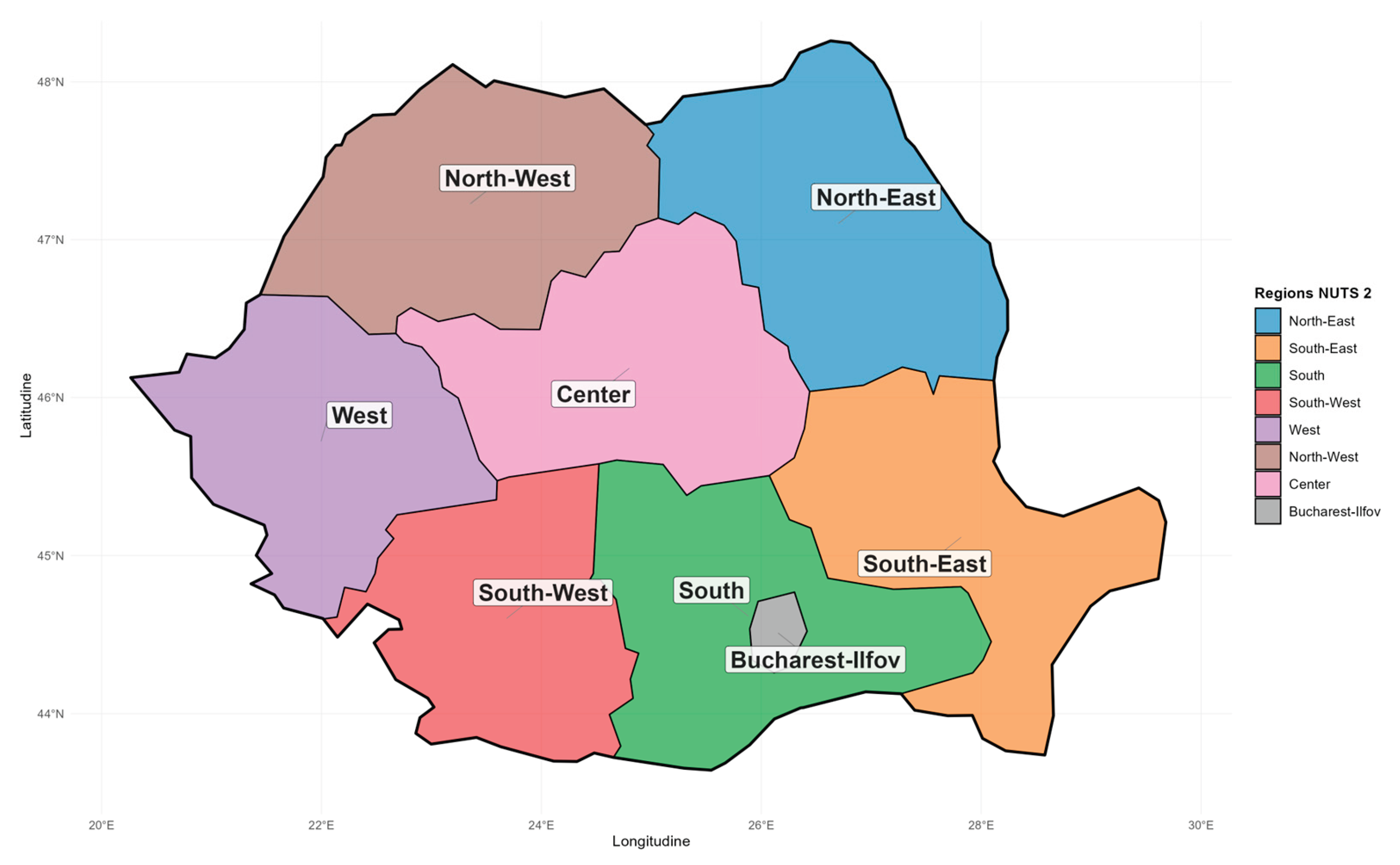
Figure 2.
Moran’s I index for rook and KNN weighted matrix.
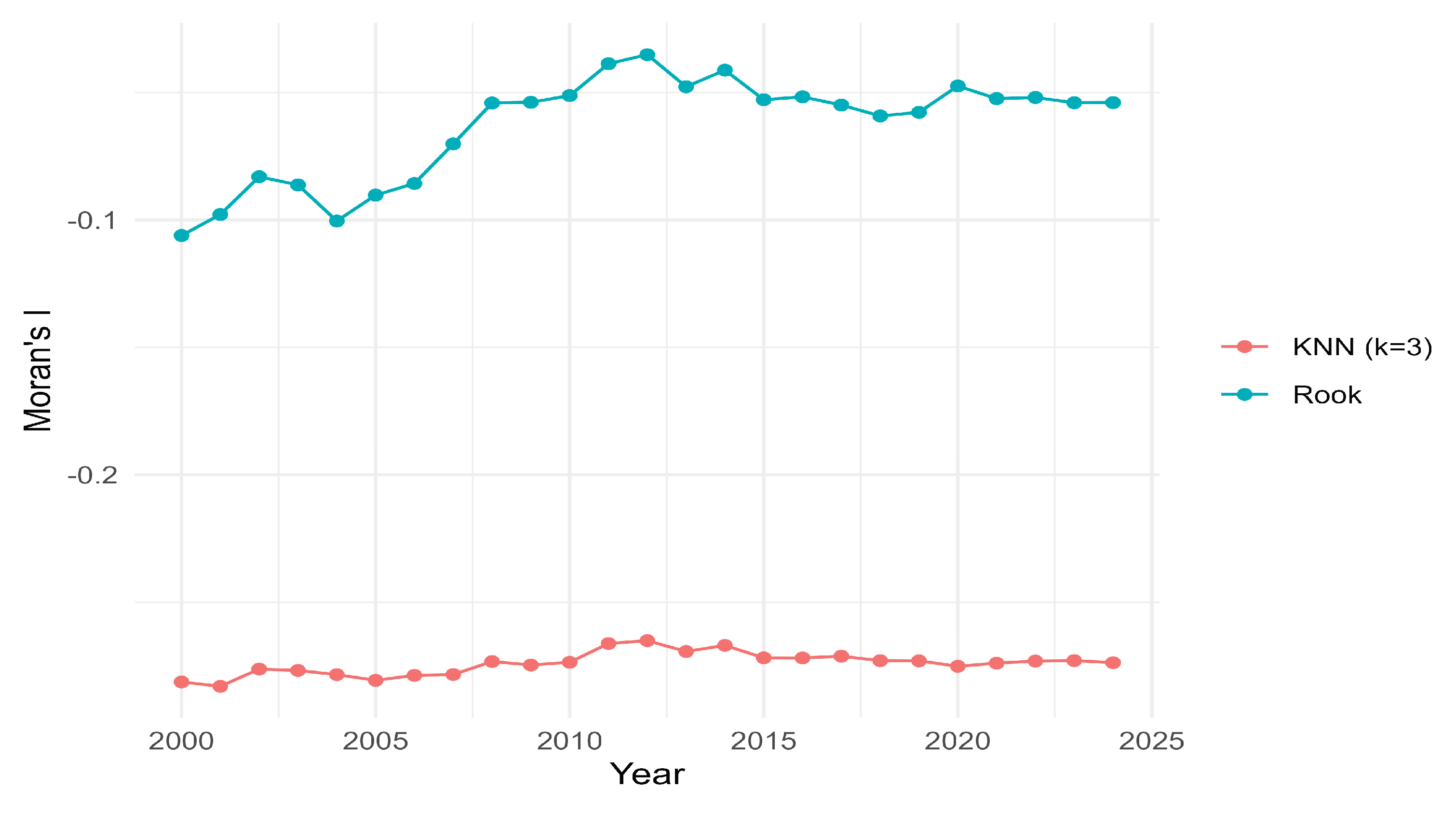
Figure 3.
Direct, indirect and total effects in SAR model.
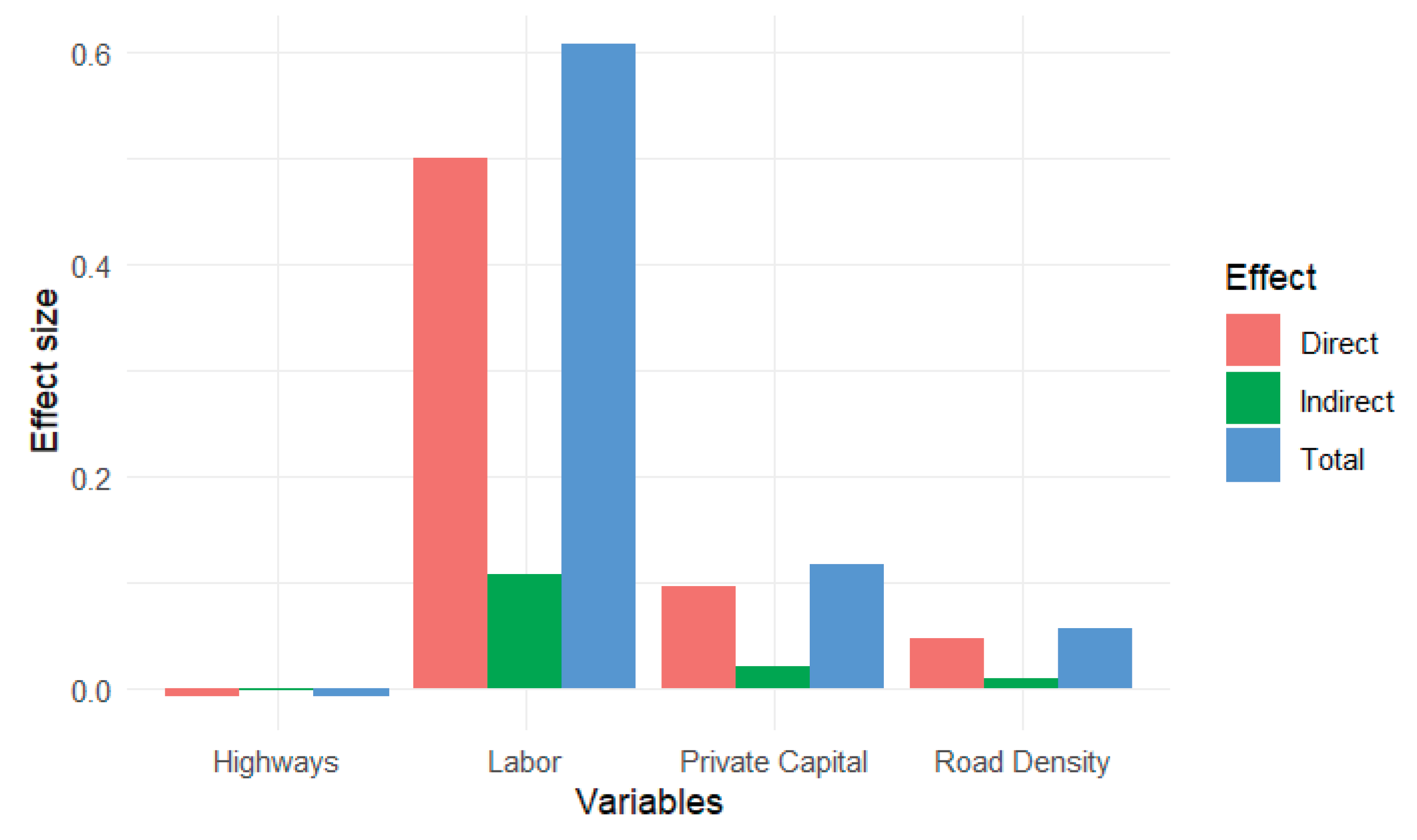

Table 1.
Definition and role of intended variables.
| Variable Name | Description | Role in the Model |
|---|---|---|
| GDPPC | Regional GDP per capita [EUR] |
Dependent variable capturing the level of regional economic performance. It reflects both productivity and income effects and serves as the main outcome influenced by infrastructure and spillover mechanisms. |
| ROADD | Road density [km / 100 km2] |
Core infrastructure variable representing the spreading of road transport networks. It depicts direct effects on regional growth through enhanced mobility of goods. It still represents the major road transport infrastructure. |
| HWAYD | Highway density [km / 1000 km2] |
Key infrastructure variable representing the availability of highway networks. It captures direct effects on regional growth through reduced transport costs and improved mobility of goods and people across national and international territory and represents the backbone for connecting to the European TEN-T network. |
| RAILD | Rail density [km / 1000 km2] |
Complementary infrastructure variable reflecting rail-based connectivity. Its effect captures alternative transport channels, particularly relevant for freight and long-distance mobility, though expected to be heterogeneous across regions. |
| PCAPIT | Private gross fixed capital formation [106 EUR] |
Private production factor control, capturing physical capital accumulation. It controls for regional investment dynamics that directly influence output and productivity. It is a major driver of development, trade flows and level of life increasing. |
| LABOR | Total regional employment | Labor input variable, representing the scale of economic activity. It accounts for differences in workforce size and supports a production-function interpretation of the model. |
| R&D | Research and development expenditure [106 EUR] |
Innovation and knowledge variable, capturing technological progress and long-term growth potential. It may also generate spatial knowledge spillovers across regions. |
| URB | Share of urban population in total population | Agglomeration proxy, capturing urban concentration effects such as economies of scale, knowledge spillovers, and labor market pooling. |
Table 2.
Regions’ data characteristics.
| Variable | Mean | Standard deviation |
Median | Min | Max | Skewness |
|---|---|---|---|---|---|---|
| GDPPC | 8014 | 7230 | 5960 | 1078 | 48,604 | 2.71 |
| ROADD | 51 | 43.1 | 36.2 | 30.7 | 178 | 2.27 |
| HWAYD | 4.52 | 8.16 | 1.52 | 0 | 57.1 | 3.10 |
| RAILD | 59.3 | 36.5 | 44.9 | 37.5 | 155 | 2.14 |
| PCAPIT | 1532 | 1745 | 970 | 185 | 12,450 | 3.45 |
| LABOR | 1015 | 161 | 947 | 785 | 1420 | 0.638 |
| R&D | 112 | 211 | 48.2 | 5.4 | 1495 | 4.23 |
| URB | 0.563 | 0.148 | 0.538 | 0.402 | 0.918 | 1.25 |
Table 3.
Variance inflation factors.
| Variable | VIF |
|---|---|
| ROADD | 10.63 |
| HWAYD | 4.59 |
| RAILD | 42.92 |
| PCAPIT | 26.82 |
| LABOR | 2.26 |
| R&D | 30.12 |
| URB | 22.30 |
Table 4.
Results of the ordinary econometric regression models.
| Variable | OLS | Fixed effects | Two-way fixed effects |
|---|---|---|---|
| ROADD | 6.435*** | 0.117*** | 0.040 |
| HWAYD | 0.128*** | - 0.032* | - 0.008 |
| LABOR | - 1.336*** | - 0.668*** | 0.508*** |
| PCAPIT | 0.771*** | 0.692*** | 0.104** |
| Adjusted R2 | 0.952 | 0.956 | 0.557 |
Significance: *** p < 0.001, ** p < 0.01, * p < 0.05.
Table 5.
LM test results.
| Model specification | LM Statistic | p-value |
|---|---|---|
| Rook-contiguity | 5.101 | 0.024 |
| KNN | 3.210 | 0.073 |
Table 6.
Spatial model selection tests.
| Test | Statistic | p-value | Interpretation |
|---|---|---|---|
| LM-Lag | 217.67 | < 0.001 | Strong spatial lag dependence |
| LM-Error | 204.75 | < 0.001 | Strong |
| Robust LM-Lag | 18.024 | < 0.001 | Lag dependence remains significant |
| Robust LM-Error | 5.101 | 0.024 | Weak but significant error dependence |
Table 7.
Spatial Autoregressive Model results.
| Variable | Coefficient |
|---|---|
| ROADD | 0.047 |
| HWAYD | - 0.006 |
| PCAPIT | 0.095* |
| LABOR | 0.496*** |
| λ | 0.185* |
Significance: *** p < 0.001, * p < 0.05.
Disclaimer/Publisher’s Note: The statements, opinions and data contained in all publications are solely those of the individual author(s) and contributor(s) and not of MDPI and/or the editor(s). MDPI and/or the editor(s) disclaim responsibility for any injury to people or property resulting from any ideas, methods, instructions or products referred to in the content. |
© 2026 by the authors. Licensee MDPI, Basel, Switzerland. This article is an open access article distributed under the terms and conditions of the Creative Commons Attribution (CC BY) license (http://creativecommons.org/licenses/by/4.0/).
Copyright: This open access article is published under a Creative Commons CC BY 4.0 license, which permit the free download, distribution, and reuse, provided that the author and preprint are cited in any reuse.


