

Submitted:
08 May 2026
Posted:
13 May 2026
You are already at the latest version
Abstract
Precise assessment of landslide potential in tectonically active mountain areas like Darjeeling Sikkim Himalaya (DSH) is a scientific challenge due to the complexity of different landslide conditioning factors that control the slope stability. Despite several studies for landslide susceptibility mapping, most of the conventional methods struggle to capture the nonlinear relationships and spatial heterogeneity that characterize landslides. Besides, the current use of pixel-based methods is insufficient to depict geomorphological units and slope-scale processes, thus limiting their effectiveness in boundary demarcation of landslide-prone areas. These limitations highlight the need for more robust machine learning frameworks that integrate geomorphology-based terrain segmentation with advanced machine learning models, which would not only facilitate modeling the multifaceted interactions among environmental components but also improve the understanding of the landslide driving forces. In this study, we have used slope unit based landslide susceptibility mapping with 4380 slope units integrated with 17 conditioning factors, and 8373 total updated inventories using six models Random Forest (RF), Generalized Additive Model (GAM), Categorical Boosting (CatBoost), Tabular Neural Network (TabNet), Bayesian Additive Regression Trees (BART), and Convolutional Neural Network (CNN). The model hyperparameters were optimized using Bayesian optimization, except for the BART model. Among the six models, RF (AUC = 0.848) and CatBoost (AUC = 0.846) were the best two performing models. Furthermore, SHAP analysis reveals that elevation, aspect, slope, distance to faults, NDVI, and proximity to roads and drainage networks are the main landslide controlling factors in DSH. The interaction analysis using SHAP indicates that the occurrence of landslides is controlled by nonlinear and threshold-dependent relations, especially among slope-rainfall, rainfall-soil moisture, and slope-distance to roads and faults, which represents a complex interaction between the hydrological triggering factor, geomorphic processes, tectonic activity, and human interventions.
Keywords:
Darjeeling Sikkim Himalaya
; slope units
; machine learning
; Bayesian optimization
; SHAP
1. Introduction
Landslides are natural phenomena in which soil, rock, or debris slides downslope under the action of gravity, resulting in significant human casualties, infrastructural damage, and ecological degradation (Alexander et al., 2005). Their initiation can be natural, such as rainfall, seismic activity, other geologic processes, and anthropogenic, such as the destabilisation of a slope by construction, mining and unplanned urbanisation, or sometimes combination of all these processes (Hungr et al., 2005). Landslides are characterized into different types such as rockfalls, debris flows, translational slides, rotational slides, and earth flows based on the type of material and movement (Varnes et al., 1978; Cruden et al., 1996).
Landslides have been considered one of the most dangerous natural processes in the world because of their high mortality rate as well as significant losses in terms of economic values. As per the International Disaster Database (EM-DAT) and the United Nations Office for Disaster Risk Reduction (UNISDR), landslides accounted for approximately 4.9% of global natural disasters, including 346 disaster events causing 66.5 billion USD global economic loss, affecting 98.6 million people, resulting in 22770 fatalities in a single 2015 year (Froude et al., 2018). From 1998 to 2017, landslides affected approximately 4.8 million people worldwide, resulting in 18,410 fatalities and approximately USD 8 billion in economic losses (Guha-Sapir et al., 2017).
The Himalayan belt of India, such as Jammu and Kashmir, Himachal Pradesh, Kumaon, Darjeeling, Sikkim, and areas of the northeast, is one of the most susceptible to landslides because the young fragile geology, the gradient is steep, the seismic activity is active, and the intensity of rainfall is high (Bhandari et al., 2006; Sidle et al., 2006). The Darjeeling Sikkim Himalaya (DSH), northeast India, is prone to landslides due to highly fractured lithology, presence of thrust belts, rapidly changing land use due to increasing tourism and population resulting in infrastructure development, and further promoting slope instability, with most of the landslides occurring in the monsoon season. Due to these reasons, it is necessary for landslide assessment, particularly in tectonically active mountain regions like the Darjeeling Sikkim Himalaya (DSH).
Landslide susceptibility mapping (LSM) is the most important step in landslide assessment because it assists in identifying the spatial likelihood of landslides by using different conditioning factors such as geological, geomorphological, topographic, hydrological, climatic, and anthropogenic. (Guzzetti et al., 2005; Reichenbach et al., 2018). Landslide susceptibility mapping (LSM) is an important tool for land-use planning, infrastructure construction, environmental management, slope stabilization, and reducing disaster risks in mountainous areas, like the Himalayas (Borrelli et al., 2018; Nsengiyumva et al., 2018).
Several mapping units are used for landslide assessment, including grid cells (pixels), terrain units, slope units, topographic units, and administrative units (Kalia, 2018; Sassa et al., 2005; Vranes et al., 1984; Reichenbach et al., 2018). However, most of the studies in the LSM are based on grid cells and slope units (Liu et al., 2023; Reichenbach et al., 2018). Of the two techniques, grid-based techniques are mostly used, which are characterized by the spatial resolution of the Digital Elevation Model (DEM), and are commonly applied in landslide susceptibility mapping because of their simplicity and ease of implementation. However, in many cases, pixel-based methods are not sufficiently able to resolve geomorphological boundaries and slope-scale processes, giving fragmented susceptibility maps that have limited physical interpretability, especially with large and complex landslides (Martinello et al., 2021). Whereas Slope units are more suitable for hydrological and geomorphological studies as they reflect the natural divisions in the topography, characterized by ridges and valleys. These units effectively capture slope-scale processes, including landslide initiation, runout, and material accumulation, along with the underlying geological environment (Alvioli et al., 2016; Martinello et al., 2021).
Recent studies on LSM have demonstrated numerous methodologies and paradigms based on deterministic, heuristic, and data-driven approaches (van Westen et al., 2006; Fell et al., 2008). The deterministic approaches are based on physical, hydrological, and geotechnical parameters to estimate the slope failure process. Although these models are meaningful, they are only applicable at a regional to national scale and sometimes confined to site-specific rather than large-scale susceptibility zonation due to the limited availability of continuous geotechnical data, which also demands high computational resources, and are strongly sensitive to uncertainty and boundary conditions (Lu et al., 2013). Heuristic approaches are mainly based on expert knowledge, geomorphological interpretation, and field-based experience, and assign weights to landslide conditioning factors based on causal relationships. Such techniques are especially beneficial in a situation where the data are scarce, the inventory quantities are limited, and for reconnaissance-level landslide assessment. However, the main weakness of these methods is that they rely on the judgment of experts and, therefore, may not allow spatial transferability when used in different physiographic and tectonic contexts (van Westen et al., 2006). Whereas, data-supported methods utilize statistical and machine-learning algorithms to define the landslide predisposition models and determine potential hazard zones by incorporation of numerous conditioning variables with landslide inventories (Pourghasemi et al., 2012; Kanungo et al., 2006; Singh et al., 2024; Ji et al., 2026).
Traditional statistical models of LSM are the Analytical Hierarchy Process, frequency ratio, the weight of evidence, logistic regression, and other approaches (Pradhan, 2010a; Bui et al., 2011; Althuwaynee et al., 2014; Chen et al., 2019; Nohani et al., 2019, Nath et al., 2021, Gupta et al., 2022, Sonker et al., 2022). Nevertheless, these techniques are limited to complex, nonlinear, threshold based and scale sensitive landslides in active mountains.
Over the past years, landslide susceptibility mapping (LSM) has shifted towards hybrid and ensemble based methods in order to address the weaknesses of individual models. Such approaches incorporate machine learning algorithms with optimization approaches or multiple learners to enhance predictive accuracy, robustness, and generalization, especially in complex mountainous environments (Tien Bui et al., 2016; Merghadi et al., 2020; Chen et al., 2020, Arabameri et al., 2019; Sahin et al., 2020; Wang et al., 2021, Pradhan et al., 2010b; Fang et al., 2021; Zhou et al., 2022; Mihu et al., 2026). According to recent literature, hybrid models such as CNN-LSTM and ensemble-based models outperform traditional techniques in modeling non-linear relationships among conditioning factors (Moghimi et al., 2024; Khouzani et al., 2025; Mao et al., 2024; Abgrami et al., 2025). Geospatial, climatic, and terrain-based variables have been identified as critical factors in improving susceptibility prediction in tectonically and geomorphologically active areas (Kainthura et al., 2021; Dutta et al., 2024; Islam et al., 2025; Birjandi et al., 2025; Rahimi et al., 2025; Dehghananari et al., 2025). Moreover, the articles based on ANN, fuzzy logic, and GIS-based models demonstrate the importance of slope gradient, lithology, rainfall, and distance to faults and infrastructure as the most influential controlling factors in landslides (Ebadati et al., 2025; Nanehkaran et al., 2023).
Although landslide susceptibility mapping (LSM) has made tremendous progress, several challenges remain, especially in difficult mountainous areas such as the Darjeeling Sikkim Himalaya (DSH). Most of the current research studies still rely on pixel-based models, which are often insufficient to describe slope-scale geomorphological and hydrological processes. Since landslides are fundamentally terrain-based processes determined by ridges, valleys, and slope morphology, pixel-based processes can result in patchy patterns of susceptibility with minimal physical meaning. Second, the accuracy of LSM relies on the quality of landslide inventories. Numerous studies depend on inventories from government organizations, and these datasets are outdated and does not contain recent landslide events which can affect the accuracy and quality of LSM. The absence of multi-source and updated inventories can have a significant impact on model performance, particularly in hilly areas where data updates are necessary. Third, even though advanced machine learning and deep learning models can make predictions much more accurately, they are usually designed to work well and are often seen as black-box systems, which makes them hard to understand and use in land use planning and hazard mitigation. Moreover, the appropriateness of various machine learning models for slope-unit representations remains under-researched, which is a crucial problem of model-data compatibility. However, slope-unit-based landslide susceptibility assessment is poorly explored in the Sikkim area, although the area is highly susceptible to landslides and has a complicated geomorphological and tectonic setting. Moreover, despite the recent studies starting to use model interpretability methods like SHapley Additive exPlanations (SHAP), the majority of them are restricted to the analysis of feature importance but do not explain the interaction effects between conditioning factors. Landslide processes are highly multivariate, arising from non-linear interactions among topographic, hydrological, structural, and anthropogenic variables, yet these interactions are often not accounted for in conventional landslide studies. The absence of SHAP-based interaction analysis limits the interpretation of threshold-dependent behavior and confounding effects between variables essential to a physically meaningful interpretation of landslide processes. Thus, it is evident that slope-unit-based modeling needs to be combined with the most recent developments in machine learning and SHAP-based interaction analysis to account for the intricate interdependencies among conditioning factors and enhance the reliability and interpretability of landslide susceptibility estimates.
To address the limitations, this work introduces a slope-unit-based landslide susceptibility mapping in the DSH relying on a high-resolution, multi-source landslide inventory and 17 conditioning factors using various machine learning algorithms, such as Random Forest (RF), Generalized Additive Model (GAM), TabNet, Bayesian Additive Regression Trees (BART) and Convolutional Neural Network (CNN) are systematically compared within a consistent modelling framework. Bayesian optimization was used to optimize the hyperparameters of these models to improve their performance. Furthermore, SHapley Additive exPlanations (SHAP) are also used to understand how conditioning factors contribute and interact with each other and allow a single model prediction to be directly related to underlying geomorphological processes. The proposed framework is expected to improve the predictive accuracy and interpretability, offering a more trustworthy and physically relevant method for assessing landslide susceptibility in complex mountainous landscapes such as the Himalayas.
2. Study Area
The Himalayan belts are among the youngest and most tectonically active mountain belts worldwide. From north to south, these active belts are characterized by a series of major tectonic discontinuities, including the South Tibetan Detachment (STD), which separates the Tethyan Himalayan Sequence from the Greater Himalayan Crystalline; the Main Central Thrust (MCT), separating the Greater Himalayan Crystalline from the Lesser Himalayan Sequence; the Main Boundary Thrust (MBT), separating the Lesser Himalayan Sequence from the Sub-Himalayan Sequence; and the Main Frontal Thrust (MFT), which separates the Sub-Himalayan Sequence from the Indo-Gangetic Plain shown in Figure. 1a (Gansser et al., 1964; Valdiya et al., 2015; Yin et al., 2006).
Darjeeling Sikkim Himalaya (DSH) is a young and tectonically active Himalayan sequence between Nepal and Bhutan (see Figure 1b). It has a topography level of between 286 m and 8586 m and an aerial cover of about 9,000km2 (Mukherjee et al., 2013). The DSH landscape is also rugged, with steep to very steep slopes, deep-cut valleys, sharp ridges, and strong gully erosion, which makes it highly vulnerable to landslides (Mandal et al., 2021). The Himalayan belt is physically subdivided into the Sub-Himalayan belt, the Lesser Himalaya, and the Higher Himalayan Crystalline belt; all of them exhibit an extremely complex tectonic regime and a rapid increase or decrease in the slope and relief (Acharyya et al., 2007; Basu et al., 2013). Geologically, all these litho-tectonic units are separated by different crustal-scale thrusts such as the Main Frontal Thrust (MFT), Main Boundary Thrust (MBT), Ramgarh Thrust, Main Central Thrust (MCT), and the South Tibetan Detachment (STD) (Beaumont et al., 2001; Mukul et al., 2000). The Lesser Himalayan Sequence primarily consists of low to medium-grade metasedimentary rocks of the Dailing Group, such as chlorite schist, phyllite, phyllitic quartzite, quartzite, dolomitic sandstone, and shale, which are fragile and weathered.
The Greater Himalayan Crystalline consists predominantly of Kanchenjunga gneiss and the Chungtang formation, which comprises high-grade metamorphic rocks such as biotite gneiss, sillimanite-garnet gneiss, and kyanite-bearing mica schist (Neogi et al., 1998; Dasgupta et al., 2004). The Southern part of the DSH consists of the Gondwana and Siwalik formations, which are predominantly composed of Sedimentary rocks such as sandstones, conglomerates, and shale (Mukul et al., 2000), whereas the Quaternary deposits of sand, silt, and clay occur along valley floors and lower slopes (Mukherjee et al., 2013).
The DSH has a humid monsoon climate, with an average precipitation of 2000-4000 mm, including 70-80% rain in the period between June and October (Govt. of West Bengal, 2017; Mandal et al., 2021). The major fluvial system of the DSH is the Tista River with its tributaries Relli, Ranikhola, and Rorochu.
As per the Indian seismic zonation map, the northern part of the DSH belongs to Zone V, but the rest of the regions are generally within Zone IV, where shallow-focus earthquakes with magnitudes ranging between Mw 4.5 and 5.5 are more frequent and a major earthquake with a magnitude of Mw 6.9 occurred on 18 September 2011, triggering landslides and reactivating the slope failures (Mukul et al., 2014, Chakraborty et al., 2011; Kellett et al., 2014).
Altogether, DSH falls under a complex tectonic regime, with a fragile geomorphology, a densely populated, infrastructurally critical landscape, steep topography, mechanically weak and weathered lithology, reactivating structural discontinuities, and intense rainfall with rapidly changing land use often produce destructive landslides (Mandal et al., 2021).
3. Dataset Used
The dataset used in the present research is presented in Table 1. We have used the PlanetScope dataset with 3m resolution from Planet Labs to generating landslide inventories. Furthermore, the previous landslide inventory was downloaded from the GSI Bhukosh portal as a point shapefile. The slope units were generated using ALOS PALSAR DEM with 12.5m resolution using GRASS GIS software downloaded from the Alaska Satellite Facility (ASF). All 17 conditioning factor maps were generated in ArcGIS Pro, using data derived from the ALOS PALSAR DEM, Bhukosh, and Google Earth Engine.
3.1. Landslide inventory
The landslide inventory dataset is the fundamental required data for the LSM, showing the information where the landslides have already occurred (Broeckx et al. 2018; Bera et al. 2021). The first landslide inventory for the DSH was obtained from the Geological Survey of India (GSI) portal (https://bhukosh.gsi.gov.in/) in point and polygon shapefile format, comprising 3,741 landslides. To maintain spatial consistency, all the landslide polygons were converted to point shapefile. To update the landslide inventory, new landslides were manually mapped using PlanetScope imagery (3 m spatial resolution) from Planet Labs (https://www.planet.com) dated 3 October 2024 under post-monsoon conditions, when landslides are best observed. The visual interpretation of geomorphological indicators, including scarps, displaced materials, bare soil, and disturbed vegetation patterns, was used to identify landslides. Further, field-based observations were used to validate the landslides and add the new landslide locations to improve the accuracy and minimize misclassification. The newly mapped landslides were also converted into point format to maintain spatial consistency. A final consolidated inventory of 8,373 landslides was prepared for the Darjeeling Sikkim Himalaya (DSH), as shown in Figure 2.
3.2. Slope Units
A slope unit is a geomorphological unit of the terrain marking out regions with homogenous slope gradient and orientation. These units are demarcated around morphological features like ridges and valleys, hence making it more precise in representing geomorphological features (Carrara et al., 1995; Alvioli et al., 2016). Slope units are more advantageous than grid-based models for landslide susceptibility mapping because they can capture the spatial heterogeneity of landslide conditioning factors (Guzzetti et al., 1999; Reichenbach et al., 2018). We generated 4830 slope units from DEM in GRASS GIS by partitioning the terrain based on slope gradient and aspect, which automatically delineated slope units (Figure 2). Out of these, 1599 slope units were consists of landslides, whereas 3231 were without landslides.
3.3. Landslide Conditioning Factors
In the present study, we have selected 17 landslide conditioning factors, including: Elevation, Aspect, Slope, Earthquake Intensity, normalized difference vegetation index (NDVI), mean annual rainfall, Lithology, Distance to Drainage, Distance to Road, Distance to Lineaments, Distance to Faults, Soil Moisture, Profile Curvature, Plan Curvature, TRI, TPI, and TWI as shown in Table 2. Furthermore, all these conditioning factors were added to slope units using zonal statistics in ArcGIS 10.8 software, where the mean values of all continuous conditioning factors were assigned to each slope unit, while for lithology, the majority class within each slope unit was considered. ALOS PALSAR DEM (12.5 m resolution) was used for the LSM, and all other conditioning factors were derived from the DEM and other platforms and further resampled to the same 12.5 m spatial resolution (Meena et al., 2022).
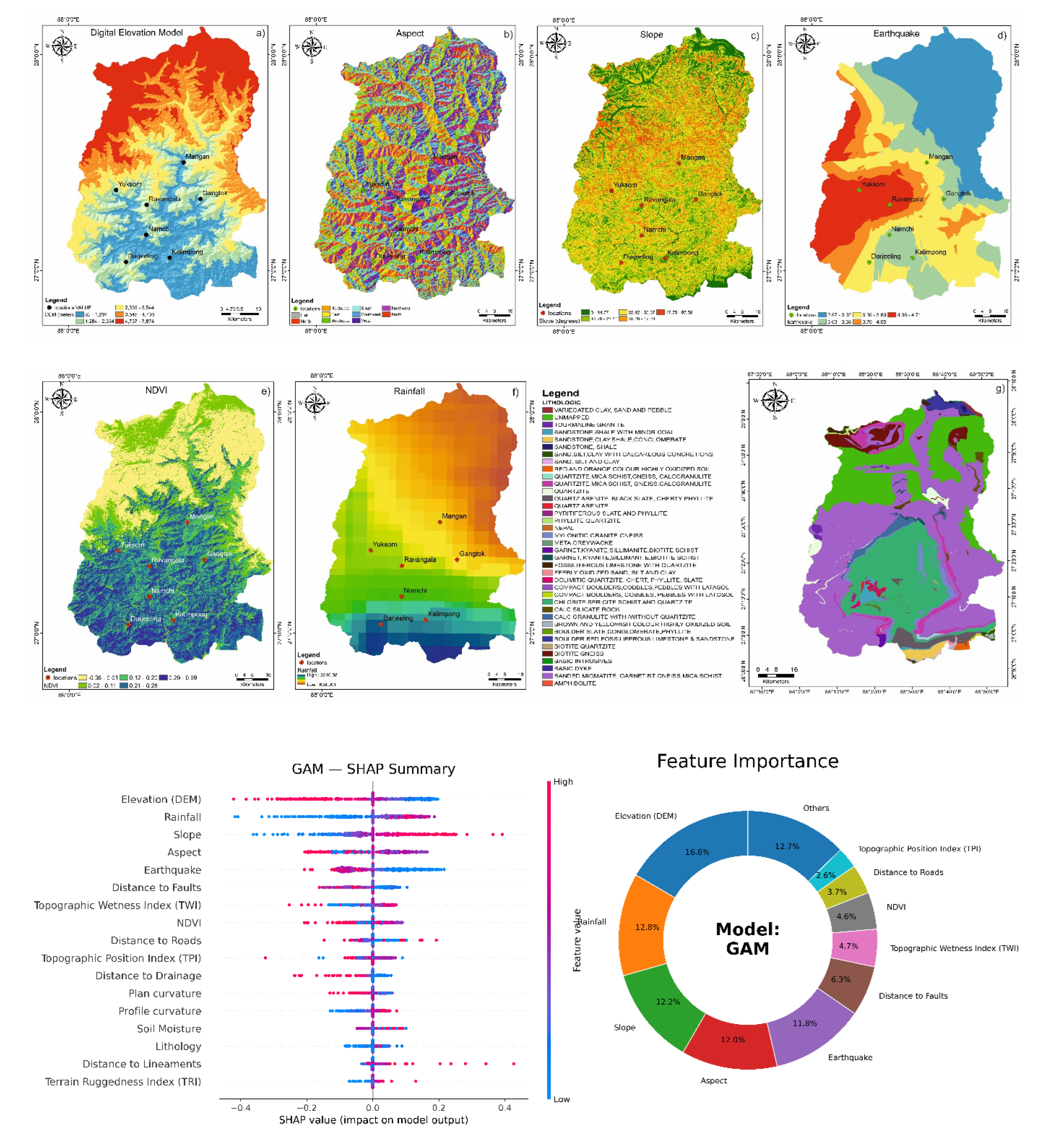
- DEM: Elevation is one of the most crucial conditioning factors of landslides because it determines weather, geomorphic processes, and terrain control which, in their turn, impacts the slope stability (Figure 3a).
- Aspect: Aspect refers to the direction of the slope face. It may have an impact on the environment, including the distribution of moisture, sunlight, and plant growth, hence a direct effect on landslides (Figure 3b).
- Slope: Slope is the inclination of the land surface, which is measured by the angle of inclination or the ratio of the shear stress to shear strength. It is a major factor that affects slope stability. The shear stress increases and stability decreases, making the landslides more susceptible (Figure 3c).
- Earthquake: Sudden seismic activities can reduce the cohesion between the rock particles by releasing sudden energy on the earth’s surface, which can also reactivate the faults, which can reduce their stability and increase the chances of landslides. Considering earthquake as one of the important conditioning factors, we downloaded earthquake data from the United States Geological Survey (USGS) and the International Seismological Centre (ISC), and with the help of the kriging process, we have generated an earthquake intensity map on the ArcGIS software by combining both of the data into a single raster layer. In this study, we have considered earthquake magnitude (Mw) values for landslide susceptibility mapping (LSM) (Figure 3d).
-
NDVI: NDVI shows the vegetation index of the area, ranging from -1 to 1. Areas with values near 1 show high vegetation zones where the likelihood of landslides is very low, as tree roots hold the soil, making it more compact and stronger, whereas NDVI values near 0 indicate very little vegetation and hence a higher likelihood of landslides. To generate the NDVI map, we used Sentinel 2 data from March 2024 with a 10-meter spatial resolution (Figure 3e). The formula for calculating NDVI is as follows:
- Rainfall: Rainfall is climate driven conditioning factors which directly influences the landslides. The water infiltrates and reduces the shear strength of rock and soil particles by increasing pore water pressure, resulting in higher chances of landslides. For LSM, we have generated mean annual precipitation data from 1980 to January 2025, downloaded from the CHIRPS (Climate Hazards Group InfraRed Precipitation with Station data) dataset, and prepared in the Google Earth Engine platform to examine the long-term mean annual rainfall. The average annual rainfall over this region is estimated at about 1575.29 mm (Figure 3f).
- Lithology: Lithology shows the source material from where landslide can occur. The DSH consists of different lithological units with different materials, mechanical strengths, and weathering characteristics. The rocks with higher shear strength resist landslides, whereas rocks with lower shear strength act as a catalyst for landslides. The lithology map was downloaded from the Geological Survey of India (GSI) Bhukosh portal. The data was prepared at a scale of 1:50,000. The study area comprised a total of 38 lithological units (Figure 3g).
- Distance to Drainage: The presence of a drainage networks, roads, faults, and lineaments increases the probability of landslides. Rivers in the mountain regions are of high erosive capacity when get in contacts with the soil and rocks, reduces their grip capacity and strength making the slope prone to failure. Selecting distance to the river we have divided the river into five categories based on the distance from the river channel to the landslide at an interval of 250m, viz. 0-250m, 250-500m, 500-750m, 750-1000m, and 1000-1250m using ArcGIS Pro (Figure 3h).
- Distance to Roads: Engineering activities, particularly road construction, disturb the natural slope conditions through excavation, cutting, and modification of drainage patterns, which reduces slope stability and induces landslides. Accordingly, the distance to roads was classified using the same 250 m interval scheme adopted for drainage proximity. The distance to road data was extracted from DivaGIS platform (Figure 3i).
- Distance to Faults and Lineaments: Faults and lineaments represent zones of weakness with high in-situ stress; due to this, the water may percolate to these weak zones, reducing their strength, and also, sometimes due to seismic activities, these zones are also the site of major slope failure as the gets reactivated. The GSI Bhukosh portal was used to acquire faults and lineaments. In case of the fault and lineament, we applied the Euclidean distance with an interval of 250m, which is equal to the distance to drainage in ArcGIS (Figure 3 j,k).
- Soil Moisture: Soil moisture is the amount of water present in the soil which can directly influence the landslide occurrence. The increase in soil moisture causes an increase in porewater pressure and reduces soil cohesion and shear strength. In the present work, we have downloaded soil moisture data from the Soil Moisture Active Passive (SMAP) satellite mission at a spatial resolution of 9 km (Figure 3l).
- Profile curvature: Profile Curvature is the inclination of the ground surface towards the downhill direction. It influences landslides by varying the surface runoff and mass movements, controlling the erosional process and slope stability of the terrain (Figure 3m).
- Plan Curvature: Plan curvature can be defined as the curvature perpendicular to the direction of slope, which controls the intersection and segregation of water runoff by controlling convergence and divergence of water flow. The area with convergent flow conditions directly controls the probability of landslides (Figure 3n).
- Topographic Roughness Index (TRI): TRI shows the surface variations by analysing the neighbouring elevation difference between different terrains. TRI values are directly proportional to landslide frequency, as the higher TRI value shows a rugged terrain surface, which increases landslide probabilities (Figure 3o).
- Topographic Position Index (TPI): TPI shows the vertical position of the terrain unit in the landscape. It differentiates between valley bottoms, slope faces, and ridgetops. Flattened topography is a common feature in low elevated places where water is likely to accumulate, making the whole area more prone to landslides (Figure 3p).
- Topographic Wetness Index (TWI): TWI shows the wetness condition of the soil at different areas. The higher value of TWI shows higher water accumulation, causing increased chances of landslides (Figure 3q). The formula for calculating TWI are as follows:
Where TCA represents Total Catchment Area.
4. Methodology
4.1. Methodology Overview
For the LSM, we selected 17 landslide conditioning factors, as shown in Figure 4, using ArcGIS software. We also selected 6 models, including RF, GAM, CatBoost, TabNet, BART, and CNN. To improve the predictive performance of all the models, we have used Bayesian Optimization to tune the hyperparameters selected for our models. For LSM slope unit based landslide inventory was used, where slope units that contained at least one landslide points were considered as landslide units and the slope units with no landslides were considered as non-landslide units. Further, the dataset with landslide and non-landslide units was divided into training and testing datasets using a stratified simple approach. The trained models generated continuous landslide susceptibility mapping values for all slope units. Further, the LSM was classified into five classes ranging from very low to very high using the natural breaks classification scheme. To determine the predictive capability of the models, we have used various statistical measures, such as confusion matrix, ROC curve, and AUC values, to determine the predictive capability of each model.
4.1.1. Random Forest (RF)
Random forest (RF) is an ensemble machine learning model that can be used for classification and regression (Breiman et al., 2001). This method is very popular and has been utilized in many remote sensing-based studies for various applications (Melville et al., 2018). RF can generate many decision trees, which can resolve the overfitting problem by using training data, resulting in more complex datasets and better performance compared to other decision trees. In the RF model, each decision tree produces an estimate, and the overall result is calculated by a voting scheme, which represents the summation of all the constituent trees; this eventually serves to build the landslide susceptibility map. The random forest is considered to be one of the most reliable and effective non-parametric ensemble learners because of its strong classification performance (Chen et al., 2017; Raju et al., 2025). The training data were further sub-divided by using the bootstrap-aggregating (bagging) method to obtain several sub-sets that had about 1/3 of the training examples. A decision tree was developed on each subset and the sum of votes of all the trees were combined to determine landslide susceptibility.
4.1.2. Generalized Additive Model (GAM)
GAM is a statistical learning model that is an extension of the generalized linear model, whereby it allows nonlinear relationships between a response variable and predictor variables (Hastie et al., 2017). Under landslide susceptibility mapping, the dependent variable is binary, which shows whether there has been a landslide event or not. Therefore, the model provides an estimation of the possibility of occurrence of landslides based on a series of environmental predictor variables.
In the landslide susceptibility analysis of Darjeeling-Sikkim Himalaya (DSH) a logistic Generalized Additive Model (GAM) was adopted which was used to explore the association between landslide occurrence and the conditioning variables selected to develop a slope-unit based susceptibility map. Under the GAM model, the smooth functions relate the response variable and the predictor variables, and hence the model is able to represent the complicated and nonlinear relationships between landslide occurrence and environmental conditions. The missing data in the dataset were imputed using median imputation before model training.
In the model specification, nonlinear relationships between the predictor variables and the occurrence of landslides were captured in smooth components The logit link function was used to estimate the chances of occurrence of landslides. To enable categorization of slope units, a decision level of 0.32 was used to differentiate landslide and non-landslide classifications. The smoothing parameter was optimized using Bayesian Optimization, and the final selected value was 0.4 to control the smoothness of the fitted functions and reduce overfitting.
4.1.3. Categorical Boosting (CatBoost)
CatBoost is a machine learning algorithm based on gradient boosting and decision trees in which many simple trees are combined to increase the predictive accuracy (Prokhorenkova et al., 2018). Unlike with many other machine learning models, the algorithm can process many different types of data including categorical variables and can give satisfactory performance even when trained with relatively small data. Another important advantage of CatBoost is the ability to reduce overfitting with the help of ordered boosting and effective preprocessing of features (Prokhorenkova et al., 2018).
The model was trained using slope-unit conditioning factors as predictors and a binary landslide presence-absence label (0 = non-landslide slope unit; 1 = landslide slope unit) and tuned it using the Bayesian optimization algorithm to improve predictive accuracy. The optimal CatBoost model had 1,703 iterations, learning rate of 0.039 and the tree depth of eight. The L2 leaf regularization was adjusted to 20.92 in order to reduce overfitting. The loss function adopted was logloss, and equal weights relating to classes were used to overcome the imbalance between the landslide and non-landslide samples. Other parameters used in the model were a random strength of 0.93, a bagging temperature of 0.80 and a count of 179 border used in discretizing the features and enhancing the stability of the model. The detailed methodology is described in Azizi and Hu (2020).
4.1.4. Tabular neural Network (TabNet)
TabNet is a deep learning architecture designed to work effectively with tabular data, combining the feature selection and representation learning properties of neural networks with the feature selection mechanisms of tree-based models. This architecture allows the model to both represent complex nonlinear relations and at the same time the most salient input features. Since landslide susceptibility mapping involves the use of structured datasets, which include several conditioning factors, TabNet is especially suited in this analysis situation.
The model carries out predictions in a series of decision steps, during which salient features are selected and transformed, through the process. Training was done using Adam optimiser and binary cross- entropy loss. The main hyperparameters have been defined as n_d=40, n_a=48, and n_steps=7, which indicate the dimensionality of features representation, as well as the number of decision steps respectively.
The sparsity regularisation parameter was adjusted to 0.0006 in order to encourage feature selection. The learning rate was set to 0.02; the batch size was 512 and the virtual batch size was 256. The gamma parameter was set to 1.74 and the mask type was taken to be Sparsemax used to select the features.
4.1.5. Bayesian Additive Regression Tree (BART)
Bayesian Additive Regression Trees (BART) is a tree-based machine learning approach, a Bayesian approach, combining a set of shallow decision trees to estimate the response to predictor variables (Marrel et al., 2009; Chipman et al., 2010; Kapelner et al., 2016; Hill et al., 2020). Within the BART paradigm, forecasts are made by summing the outputs of several trees and thus allow the model to reflect non-linear and complex relationships between landslides conditioning factors and landslide occurrence. The contribution of each of the trees to the ultimate prediction is small and encourages a check on complexity in models and reduces overfitting.
The BART model has been used to examine the association between the landslide occurrence and the chosen conditioning factors in the present study of slope-unit-based landslide susceptibility mapping. The Bayesian model parameters are estimated using the Markov Chain Monte Carlo (MCMC) sampling technique and hence enable the model to capture predictive uncertainty.
The selection of the main hyperparameters in this study was the number of trees 200 (n_trees 200), the burn-in 200 (n_burn 200), the number of posterior draws 800 (n_samples 800) and the number of parallel chains 4 (n_chains 4) to improve the stability and convergence of the estimation. These hyperparameters were chosen based on commonly adopted values reported in the literature, ensuring stable MCMC convergence and reliable posterior estimation.
4.1.6. Convolutional Neural Network (CNN)
The convolutional neural network (CNN) technique is one of the most famous deep learning models. This model can rapidly process diverse data types, such as tabular and sequential data (LeCun et al., 2015; Yamashita et al., 2018). Sometimes, CNN-based models often outperform ensemble learning models (Perol et al., 2018). In this study, a one-dimensional (1D) CNN was selected, in which each slope unit was considered as one-dimensional, containing all the conditioning factors. The 1D convolutional neural network model consisted of two convolutional layers which had 32 and 96 filters respectively and used a kernel size of 3. One pooling layer and a fully connected layer that consisted of 64 units were added to identify the feature pattern related to the presence of landslides. The pooling operation decreases the size of the feature maps thus, increasing the efficiency in computation (LeCun et al., 2015). To add nonlinearity to the model, Rectified Linear Unit (ReLU) activations was introduced (Wang et al., 2019). To minimize overfitting, dropout with a rate of 0.599 was added to the fully connected layer. For model training, we have implemented a learning rate of 0.00136, with a batch size of 128 and a weight decay of 3.22 × 10⁻⁵. For input preparation mean value of all the conditioning factors were added to each slope unit. In the case of lithology, we have used the dominant class for each slope unit.
4.2. SHAP
In the study, we used SHapley Additive exPlanations (SHAP) to understand how the models make predictions for landslide susceptibility mapping. SHAP is a model interpretation method based on cooperative game theory that explains the role of each conditioning factor’s contribution to the prediction of the model (Wen et al., 2024). SHAP calculates the Shapley values that show how much each factor contributes to the model’s prediction by including and excluding the variables (Li et al., 2024).
In the model, if the prediction changes significantly, the factor is considered important, whereas if the prediction changes very little, then that factor is considered less important. SHAP repeats this process by testing all factors together in many different combinations of factors, resulting in getting the average contribution of these factors for LSM.
SHAP assigns the contribution value to each conditioning factor used in the model for each slope unit. SHAP with positive values reflects that the factor strongly influences the landslide susceptibility, whereas a negative SHAP value influences the landslide susceptibility less (Meng et al., 2020).
This method provides better understanding of complex models by analyzing different landslide conditioning factors. Implementation of SHAP can be helpful to the scientific community and government bodies for landslide assessment, landuse planning and landslide risk reduction.
The SHAP value for a feature can be expressed as:
Where represents the Shapley value of the feature , is the set of all features, is a subset of features excluding feature , and represents the model prediction using the subset of features.
4.3. Hyperparameter Extraction Using Bayesian Optimization
For LSM using different methods, it is crucial to configure hyperparameters in order to improve the model’s predictive performance (Morales-Hern’andez et al., 2023). In the present study, we have used the Bayesian Optimization (BO) method to find out the optimal hyperparameter values for the selected models. BO was applied to all models except the BART model, as it was implemented without any external hyperparameter tuning, as the BART model controls its complexity through its built-in Bayesian framework. BO efficiently searches the hyperparameter space by testing different combinations of parameters and selecting the best set for the models. Unlike the conventional methods of hyperparameter optimization such as grid search and random search, the method gives a focus on potential ranges of parameters that are promising and thus increases the overall optimization procedure. Bayesian optimization was performed using the Optuna framework to optimize the models’ hyperparameters.
The model performance was measured using five-fold stratified cross-validation, and the optimization metric was ROC-AUC. The best hyperparameter settings produced in this process were then used to train the final models. The resultant values of hyperparameters of each algorithm are presented in Table 3.
4.4. Model Accuracy Evaluation Metrics
The present study quantifies the LSM model’s performance using metrics such as the confusion matrix, the ROC curve, and the AUC. The confusion matrix shows the visual summary of the performance of the model at different categories showing classifying accuracy by classifying it into true positives (TP), true negatives (TN), false positives (FP), and false negatives (FN) (Riehl et al., 2023). These are important for determining the model’s performance on validation sets.
Whereas ROC curve shows the model’s capacity to differentiate landslide and non-landslide zones by plotting true positive rate (TPR) and the false positive rate (FPR).
When the ROC curve is near top left side indicates the better performance of the model with higher accuracy. The AUC value close to 1 indicates higher classification performance at different threshold values (Roumeliotis et al., 2024). We have also validated the model’s performance using Precision, Recall, and F1-score methods have been employed to validate the model’s performance (Nadim et al., 2023).
5. Results
5.1. Feature Importance of Landslide Conditioning Factors
Landslides are driven by different conditioning factors that are need to be determined to assess their role in relation to landslides. In the present work, we have used SHAP to establish the contextual relationship between landslides and its conditioning factors, which is most popular for interpretability of different machine learning models for LSM (Hu et al., 2023). Figure 5 represents the beeswarm plot showing all 17 conditioning factors on left side in decreasing order from top to bottom, with the donut showing the top 10 most contributing conditioning factors by quantity on the right side.
The RF model showed strong relationship with individual predictors: precent wise contribution of top ten factors are as follows: DEM (18%), aspect (14.5%), NDVI (13.5%), distance to faults (11.4%), slope (8%), soil moisture (5.6%), distance to roads and drainage (5.1%, 4.9%), rainfall (3%), TWI (2.7%), and rest of the factors contributed 13.4% among all the 17 conditioning factors, indicating that the landslides are mostly controlled by topographic, and anthropogenic factors (Figure 5a).
Whereas top ten feature importance using CatBoost are as follows: DEM (13.5%), aspect (13.3%), distance to faults (11.4%), slope (10.2%), distance to roads (6.5%), distance to drainage (6.5%), NDVI (6.4%), TPI (4.9%), Rainfall (2.9%), soil moisture (4.5%), and rest of the factors contributed 19.3% indicating landslides are mostly influenced by topographic, structural as well as anthropogenic factors (Figure 5b).
The relationship between landslides and conditioning factors in the GAM model was quite smooth, as expected of a semi-parametric model. The feature contributions suggest that the dominant factors are elevation (DEM) (16.6%), rainfall (12.8%), slope (12.2%) and aspect (12.0%). Earthquake (11.8%) and distance to faults (6.3%) are also important, followed by TWI (4.7%), NDVI (4.6%) and distance to roads (3.7%). The other factors collectively contribute about 12.7% of the total contribution. The findings indicate that the GAM model accounts for a balanced contribution of topographic, hydrologic and structural features, with a gradual change of feature contributions compared to tree-based models (Figure 5c).
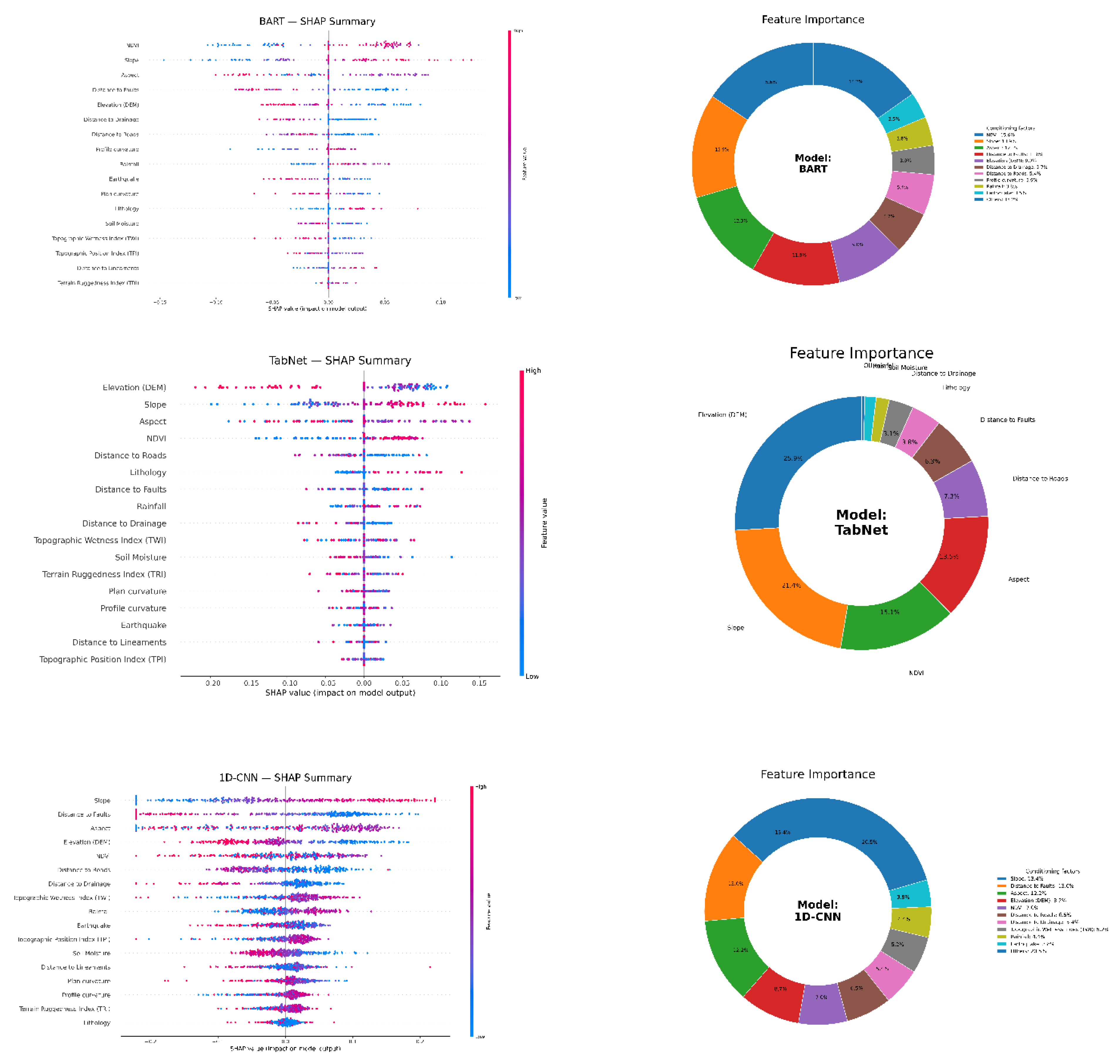
The BART model exhibits a distinct feature contribution, reflecting its nature as a probabilistic ensemble model. The dominant factors include NDVI (15.2%), slope (13.8%), and aspect (12.7%), followed by distance to faults (11.8%) and elevation (DEM) (11.5%). Distance to drainage (6.7%), rainfall (5.7%) and curvature factors are also important. Other factors account for approximately 13.7%. The findings suggest that the BART model gives more weight to vegetation and slope related factors, and hence comparatively larger clustering of the susceptibility patterns (Figure 5d).
The TabNet model shows strong reliance on a handful of important features based on its attentive feature selection. Elevation (DEM) (25.8%) and slope (21.4%) contribute the most, followed by NDVI (15.1%) and aspect (13.3%). Distance to roads (7.1%) and distance to faults (6.3%) are moderately significant, with rainfall, curvature and other factors less significant. The rest of the factors contribute to a small fraction. This suggests that TabNet considers major geomorphological and vegetation factors, while downplaying other features (Figure 5e).
The CNN model has a relatively even distribution of factor importance, which is consistent with the feature extraction power of deep learning models. Elevation (DEM) (16.6%), slope (14.4%), and aspect (12.3%) are the most influential factors, followed by NDVI (9.7%) and distance to faults (7.6%). Distance to drainage (6.5%), rainfall (6.3%) and TWI (5.7%) also play a moderate role. Other factors contribute a total of 14.9%. This suggests that CNN accounts for complex interactions between multiple conditioning factors, leading to a more equal contribution pattern than the other models (Figure 5f).
Based on the result, it is observed that both the model shows significant differences in their dependence on each landslide controlling factors. The landslides in DSH are controlled by morphometric, anthropogenic, and structural factors. All the model performed well, showing their strong feature selection capabilities for LSM prediction.
5.2. SHAP Interaction Analysis of Landslide Conditioning Factors
To further explain how the conditioning factors interact to cause landslide susceptibility, SHapley Additive exPlanations (SHAP) interaction analysis was performed using the Random Forest (RF) model, which performed best among the tested models and was further used to explain the combination effect of the conditioning factors (See Figure 6). In contrast to individual feature importance, interaction analysis can reveal how the contribution of one variable is conditioned by another, providing insight into the nonlinear and coupled processes that control landslide susceptibility.
The pairs of conditioning factors selected for interaction analysis were based on a combination of SHAP rankings from the top two models, RF and CatBoost, and the geomorphological interpretability of the interactions. Even though variables such as elevation, aspect, and distance to faults had higher SHAP importance, they are mainly indirect or proxy controls and are less applicable to interaction-based physical interpretation. In Contrast, slope was consistently found to be an effective variable in both models, and it is the most unambiguous predisposing factor governing gravitational instability. SHAP dependence patterns also suggest that several variables, such as rainfall, soil moisture, and proximity-based variables, exhibit significant effects in most cases when conditioned with slope. So, slope was chosen as the main interaction variable to study how triggering and modifying factors affect landslide occurrence.
The findings indicate that landslide susceptibility in the study area is governed by highly nonlinear, threshold-sensitive interactions, with slope as a determinant of terrain stability and other variables as conditional triggers or modifiers.
5.2.1. Slope–Rainfall Interaction
The slope-rainfall relationship shows a clear nonlinear trend, in which landslide susceptibility is influenced by both rainfall and slope (Figure 6a). At lower slope angles (<15°), SHAP values are predominantly negative, regardless of high precipitation intensity, indicating stable conditions even under high precipitation. However, at ~20–30°, increasing rainfall is associated with positive SHAP values, indicating a rapid rise in instability. This trend shows that rainfall is the primary triggering factor, with its effect significant when the slope angle is moderate to high. The observed interaction is consistent with geomorphological processes, in which intense precipitation increases pore-water pressure and reduces effective shear strength, resulting in landslides along steep slopes.
5.2.2. Slope–Distance to Roads Interaction
The slope-distance to roads interaction highlights the contribution of anthropogenic disturbances to the fluctuation of slope stability (Figure 6b). Regions near roads have higher SHAP contributions, especially on moderate to steep slope gradients, but road proximity has less impact in low-slope regions. This pattern indicates that terrain steepness strongly controls the destabilizing effect of roads. Road construction activities, such as slope cutting and toe removal, increase the instability of steep slopes, indicating that anthropogenic factors are secondary triggers rather than independent controls.
5.2.3. Slope–Distance to Drainage Interaction
The slope-distance to drainage interaction shows a moderate yet consistent trend, where slope units near drainage channels have a slightly higher SHAP contribution at moderate to high slope values (Figure 6c). This indicates that the effect of the fluvial processes, such as toe erosion and undercutting, reduces slope stability and increases the landslide susceptibility.
However, the effect of drainage is comparatively less than that of rainfall and road-related interactions, indicating that it is a secondary geomorphic modifier.
5.2.4. Rainfall–Soil Moisture Interaction
The interaction between precipitation and soil moisture shows that the precipitation effect is strongly dependent on the antecedent moisture conditions. Rainfall shows a stronger relationship at higher soil moisture levels, as indicated by higher SHAP values (Figure 6d).
This trend highlights hydrological preconditioning, in which already saturated soils are more prone to slope failure with an increase in rainfall. It indicates that the onset of landslides is not only governed by the precipitation rate at a particular time but also by the state of the moisture, which weakens the terrain.
5.2.5. Slope-Distance to Fault Interaction
The relationship between slope and distance to faults is nonlinear. SHAP contributions are higher in areas closer to faults, especially when the slope is moderate to high (Figure 6e). SHAP values are inversely proportional to distance to faults; as distance to faults increases, landslide susceptibility decreases. This implies that tectonic structures significantly affect the landslide occurrence by weakening the rock mass due to the presence of fractures and structural discontinuities. Whereas slope remains the primary factor that controls landslides. Being close to faults makes landslides more likely by making materials weaker and making them more likely to fail on steep terrain. Overall, the interaction analysis shows that topographic, hydrological, anthropogenic, and structural factors interact to control landslide susceptibility in the study area. The main control is the slope, which determines the stability of the baseline, whereas rainfall is the primary triggering factor. This baseline condition is modulated by other factors such as soil moisture, proximity to roads, drainage, and faults under certain conditions. These findings indicate that landslide processes are inherently multivariate, nonlinear, and threshold-sensitive, necessitating the consideration of interaction effects to improve susceptibility modeling and risk assessment in mountainous environments.
5.3. Comparison of Landslide Susceptibility Models
The landslide susceptibility map (LSM) using Random Forest (RF), Generalized Additive Model (GAM), CatBoost, TabNet, BART and CNN for DSH based on a slope unit was developed in the Visual Studio platform and the map was prepared in ArcGIS 10.8. The results of all six LSM models were classified into five classes using equal interval classification (Figure 7). The LSM maps were classified into very low to very high zones, coloured dark green, green, yellow, orange, and red, respectively.
The results indicated that the high zones of susceptibility are more prominent in the central-southern part of DSH (Darjeeling, Kalimpong, Gangtok, Namchi, Ravangla, Pelling, Yuksom, Mangan, Dikchu, Jorethang and surrounding region) and the low susceptibility is mostly observed in the northern part. The high susceptibility pattern is associated with the presence of roads and the erosive capacity of the Tista River as well as the high rainfall in these areas, suggesting that landslides are due to the combination of both hydrologic and anthropogenic interference. On the other hand, the northern part remains mostly snow-covered with minimal human activities, hence low susceptibility.
The models have well predicted the landslide susceptible slope units. All models have shown a similar but with a certain level of variation in susceptibility pattern. A majority of the slope units are in very low to low classes, which are very few in landslide occurrence (Figure 6), whereas high to very high slope units are more in occurrence of landslides.
The northern part of the area was reported as the least affected in literature due to a lack of inventory. But in this study, all models have identified landslide areas in the northern part along the river beds due to the inclusion of new landslides along with historical inventories, which indicates the importance of updated inventories.
Figure 8 illustrates the number of landslides for different susceptibility zones, the number of slope units (blue bars) and the percentage of landslides for each unit (orange bars). The blue bars represent the number of slope units, orange bars indicate the percentage of landslides, and the green dashed line indicates the percentage of area of each susceptibility zone. All the models follow a trend of most landslides being located in the high to very high susceptibility classes, even though the percentage of area under this class is lower. This suggests that the models have well separated landslide and non-landslide slope units.
The RF model indicated that the highest number of slope units was in the very low class (1712), followed by low (992), moderate (679), high (797) and very high (650). The distribution pattern of landslides shows that only 1.0% and 3.6% of landslides are found in the very low and low classes, respectively, 13.0% in the moderate class, and the largest percentage of landslides in the high (42.7%) and very high (39.6%) classes.
The CatBoost model indicates the highest number of landslides in the very high class. The very low class has the highest number of slope units (2166), followed by very high (1388), low (782), moderate (253) and high (241). The very high class has the highest concentration of landslides (82.6%), while the very low, low, moderate, and high classes have just 1.6%, 3.2%, 4.8%, and 7.8% of landslides, respectively.
The GAM model reveals a gradual increase from lower to higher classes, with the very low (1890) being the most predominant class, followed by low (877), moderate (856), high (754), and very high (453). The proportion of landslides increases from lower to higher classes, 5.8% in very low, 15.1% in low, 24.3% in moderate, 31.9% in high and 22.8% in very high class.
The TabNet model indicates 1557 slope units in very low class, 1222 in high, 843 in moderate, 743 in very high and 465 in low class. The landslide distribution shows that 3.8% and 5.8% of landslides are in very low and low classes, respectively, 17.5% in moderate class, while high and very high classes have the highest number of landslides, 39.5% and 33.5% respectively.
The landslide distribution in the BART model is different with a higher proportion of landslides falling in moderate to high classes, showing lower spatial discrimination. The greatest number of slope units was observed in high class (1643), followed by moderate (1486), low (1034), very low (338) and very high (329). The highest percentage of landslides are found in high class (58.4%), moderate (22.5%) and very high (16.9%) classes, while the very low and low class contain 0.0% and 2.2% of landslides, respectively.
The CNN model indicates that the highest number of slope units is observed in very low class (2228), followed by low (786), moderate (789), high (673) and very high (354). The landslide distribution shows that 7.1% and 14.4% of landslides are in very low and low class, respectively, 25.9% in moderate class, and the highest proportion in high (31.8%) and very high (20.8%) class.
In general, the high proportion of landslides in high to very high susceptibility classes in all the models indicates the suitability of the slope unit-based LSM approach and the conditioning factors selected in this study.
5.4. Model Accuracy Evaluation
For LSM in DSH, we selected six models: Random Forest (RF), Generalized Additive Model (GAM), CatBoost, TabNet, Bayesian Additive Regression Trees (BART), and Convolutional Neural Network (CNN). All these models were analyzed using an independent slope unit based test data set. The AUC-ROC curve indicating model accuracy is shown in Figure 8 for all the selected models. All six models performed well in differentiating between landslides and non-landslide slope units with an AUC value ranging from 0.82 to 0.848. In DSH, among all six models, RF scored the highest AUC value (0.848), CatBoost scored the second with an AUC value of 0.846, followed by GAM (0.837), CNN (0.831), BART (0.831), and TabNet (0.82) scored the least among all six models. However, all the models have achieved AUC values greater than 0.80, indicating better discrimination and slope-unit-based landslide prediction. The classification performance metrics highlight differences in model behavior.
Random forest achieved the most balanced performance (precision = 0.606, recall = 0.808) and the highest F1 score (0.691) among the six models. CatBoost (0.682) and CNN (0.673) showed stable performance. The confusion matrix of each model is presented in Table 5. Random Forest correctly classified 388 landslide units and 717 stable slope units, with 252 false positives and 92 false negatives, indicating balanced performance. Whereas, GAM and TabNet detected the largest number of landslide units with higher recall values but also higher false positives. CatBoost and BART classified the largest number of stable slope units, showing more conservative predictions. However, CNN showed intermediate behaviour between these approaches.
These results suggest that although individual performance measures vary across models, all models provide reliable landslide susceptibility estimates, with RF and CatBoost being the most effective approaches for slope-unit-based landslide susceptibility mapping.

Table 4.
Comparative performance of landslide susceptibility models at the slope-unit scale.
| Model | AUC-ROC | Accuracy | Precision | Recall | F1-score |
|---|---|---|---|---|---|
| Random Forest | 0.848 | 0.761 | 0.606 | 0.808 | 0.691 |
| GAM | 0.837 | 0.742 | 0.576 | 0.843 | 0.684 |
| CatBoost | 0.845 | 0.746 | 0.583 | 0.822 | 0.682 |
| TabNet | 0.82 | 0.719 | 0.549 | 0.852 | 0.668 |
| BART | 0.831 | 0.756 | 0.667 | 0.527 | 0.589 |
| CNN | 0.831 | 0.746 | 0.587 | 0.787 | 0.673 |
Table 5.
Confusion matrix results showing the classification performance of the six models for landslide susceptibility mapping, including true negatives (TN), false positives (FP), false negatives (FN), and true positives (TP).
Table 5.
Confusion matrix results showing the classification performance of the six models for landslide susceptibility mapping, including true negatives (TN), false positives (FP), false negatives (FN), and true positives (TP).
| Model | TN | FP | FN | TP |
|---|---|---|---|---|
| Random Forest | 717 | 252 | 92 | 388 |
| GAM | 671 | 298 | 75 | 405 |
| CatBoost | 780 | 189 | 150 | 330 |
| TabNet | 634 | 335 | 72 | 408 |
| BART | 779 | 190 | 152 | 328 |
| CNN | 704 | 265 | 102 | 378 |
6. Discussions
The current paper developed a slope-unit-based landslide susceptibility model (LSM) for the Darjeeling-Sikkim Himalaya (DSH) using six machine learning and deep learning models (Figure 7); all of these models performed well with AUC values greater than 0.80 (see Table 4,5). Among the selected models, Random Forest (AUC = 0.848) and CatBoost (AUC = 0.846) were the best performing model as shown in Figure 9, because of their ability to capture nonlinear relationships and higher order interactions between the landslide conditioning factors. In contrast, the transition to susceptibility was smoother in GAM and TabNet, since they are more likely to generalize relationships. BART showed a conservative predictive behavior, and CNN also under performed due to their inability to extract slope-unit-based tabular data when spatial features were limited. The SHAP based feature importance shows that in DSH, the landslide is affected by DEM (18%), aspect (14.5%), NDVI (13.5%), distance to faults (11.4%), slope (8%), soil moisture (5.6%), distance to roads and drainage (5.1%, 4.9%), rainfall (3%), TWI (2.7%) (see Figure 5).
Figure 4.
SHAP summary plots and corresponding feature importance charts for (c) GAM, (d) BART, (e) TabNet, (f) 1D-CNN used in landslide susceptibility mapping.
Figure 4.
SHAP summary plots and corresponding feature importance charts for (c) GAM, (d) BART, (e) TabNet, (f) 1D-CNN used in landslide susceptibility mapping.
In RF, around 30% of slope units fall under high to very high zones, whereas CatBoost detected 40% of slope units under high and very high zones (Figure 5). RF showed that among the 17 factors, elevation, aspect, NDVI, distance to faults, and slope are the five most controlling factors for landslides.
The LSM result shows that most of the landslide susceptibility zones were concentrated in the southern and central parts of DSH, as shown in Figure 7, which experiences the most intense monsoonal rainfall and fluvial dominated processes, and the northern area is mostly affected by glacial and cryogenic processes with very little anthropogenic activity (Starkel et al., 2014; Kashyap et al., 2021; Biswakarma et al., 2023; Prasad et al., 2021; Sonker et al. 2021; Kashyap et al., 2024). The Darjeeling, Kalimpong, South Sikkim and adjacent areas also receives very high monsoon rainfall (up to 5000-6000 mm/year) and frequent short duration high intensity rainfall (200-400 mm/few hours), which may cause debris flows and slope failures (Nath et al., 2021; Singh et al., 2021; Ram et al., 2022; Riaz et al., 2023).
However, from south to north, rainfall decreases, but landslides still take place across the region except the glacier covered norther parts, suggesting that rainfall is one of the most important factor triggering landslides (Bhandari et al., 2021; Sonker et al., 2021; Kashyap et al., 2024). Due to the updated landslide inventory, we have also observed landslide susceptible zones in the northern part of the study area along the river corridors which were lacking in the previous studies.
The SHAP-based interaction provides a better understanding of the physical processes that determine landslide occurrence and shows that nonlinear, threshold-dependent interactions, rather than individual factor effects, control susceptibility. Slope is the primary predisposing variable that governs the instability of the terrain at the base, while the other variables are conditioning triggers or modifiers. The slope-rainfall interaction exhibits a distinct threshold behavior, in which moderate slope gradients (~20–30°) and steeper gradients significantly increase landslide susceptibility to rainfall (see Figure 6a). Such behavior reflects the physical mechanism of pore-water pressure buildup and rapid reduction in effective shear strength under saturated conditions.
Moreover, the interaction of rainfall and soil moisture emphasizes the significance of hydrological preconditioning, which is consistent with the high infiltration rate of sandy and silty regolith in the area, and thus slopes are highly susceptible to mass movements during the duration or even the intensive rainfall (Figure 6d) (Chowdhuri et al., 2020; Saleem et al., 2020; Nath et al., 2021). The presence of the Tista River also contributes to slope instability in DSH. The river is in the youth stage, where it is capable of high erosion capacity and comprises deeply incised valleys (∼1000–3000 m) and steep gradient channel, which increases lateral erosion, resulting in frequent undercutting of slope toes, thereby increasing slope instability in the DSH (Scherler et al., 2015; Ghimire et al., 2020).
Seasonal fluctuations in the increase or decrease in river discharge especially in heavy rainfall and snowmelt conditions, increase the pore water pressure and reduce the shear strength, resulting in landslides (Pathak et al., 2016; Ghimire et al., 2024). Moreover, geomorphic processes such as alluvial fans, channel migration, and sediment aggradation indicate ongoing landscape realignment, which further increases the vulnerability of drainage-proximate areas. These are the processes that are directly related to the high SHAP contributions near drainage networks.
Anthropogenic factors contribute to natural instability, which is seen in the slope-distance to roads interaction (Figure 6b). Road construction and deforestation, along with changes in land use, have intensified geomorphic processes by altering natural drainage patterns, increasing surface runoff, and destabilizing slopes through excavation and toe removal. Consequently, high-susceptibility zones are consistently aligned along road corridors, implying interaction between geomorphic and human-generated disturbances.
The slope-distance to faults interaction demonstrates the significance of tectonic controls (Figure 6d), with proximity to faults and thrusts weakening the rock mass through fracturing and structural discontinuities, suggesting that the Himalayan region is tectonically active with continuous uplift and under a complex surface deformation process, increasing landslide frequencies. The major structural discontinuities that affect the landslides are Geilkhola fault, Martam fault, Munsiari thrust, Ramgarh thrust.
All this evidence suggests that a combination of topographic, hydrological, structural, and anthropogenic factors determines landslides in the DSH. The Himalaya is under a complex tectonic regime, which is active and continuously uplifting, with deformations causing slope instabilities. All these results support the argument that the landslides in the DSH are indeed a complex interaction of topographic, hydrological, structural, and anthropogenic factors.
The results of the current research are consistent with the results of the previous works which show that the influence of rainfall, geology, and geomorphology are the most significant factors causing landslides in the Himalayan scenery (Mandal et al., 2018; Das et al., 2019; Nath et al., 2021), and also allow affirming that the impact of monsoonal precipitation Nevertheless, unlike the literature, which emphasizes the predominance of individual factors, the present study confirms that the effects of interaction are predominant in landslide susceptibility that can be better captured by both slope unit-based models and landslide ensemble machine learning approaches.
Past literature suggested conflicting findings on the predictive accuracy of bivariate and machine learning models, with some studies presenting superiority of statistical models and others showing the superior performance of machine learning models (Kadavi et al., 2018; Lee et al., 2018; Huang et al., 2020; Zhang et al., 2020; Barbosa et al., 2021; Bera et al. 2021; Rahaman et al. 2021; Bachri et al. 2021). Our current study shows that ensemble based machine learning models like Random Forest and CatBoost have better predictive capability because they non-linearly relate and interact with conditioning factors.
The overall findings suggest that the multivariate, nonlinear, and threshold-dependent processes govern the landslide susceptibility in the DSH with slope being one of the most important determinants of landslide base stability, rainfall being the most important triggering factor, and soil moisture, drainage, roads, and tectonic structure as modulators of susceptibility in certain circumstances. Combining slope unit-based modeling with SHAP-based interpretability is a physically meaningful and sound framework for understanding landslide processes and provides valuable information for effective landslide risk management in complex mountainous terrain.
7. Limitations and Constraints
Landslides in the DSH are complex phenomena that are triggered by multiple factors, and our study provides valuable insights into LSM. However, these factors are driven by static as well as dynamic conditioning factors, whereas in the present approach, we have considered static conditioning factors only, which can limit the quality of LSM. All these conditioning factors were sourced from freely available multi-sensor data with different resolutions and data types (raster and vector), which can cause problem in data compatibility and model validation. The inventories were manually mapped and were not automatically determined, which can add human error in the generation of a precise inventory, and LSM quality can be compromised (Singh et al., 2025; Chandra et al., 2025a; Chandra et al., 2025b). The delineation of slope units is dependent on the selection of threshold parameters controlling flow accumulation and contributing area, which may influence the number and size of the resulting units. Although multiple threshold values were tested and the final configuration was selected based on geomorphological consistency, a detailed quantitative sensitivity analysis was not performed. This limitation may introduce some uncertainty in the spatial configuration of susceptibility zones and is considered a scope for future work. Even though the slope unit-based method minimizes the clustering effect of landslide inventory points, residual spatial autocorrelation may still persist among adjacent slope units. Conventional cross-validation might be used instead of spatially explicit validation methods, and, as such, it may introduce some level of optimistic bias into model performance estimates. The best way forward is to implement spatial cross-validation structures to better represent spatial dependency and increase model reliability.
The integration of InSAR-based results can detect and provide the current deformation rates of the area at a higher precision (Singh et al., 2022; Bhasin et al., 2023). In the present work, we have considered all the landslide in point shapefile format of the same intensity, whereas they may have different magnitude and types. The present work is totally based on multi-sensor data which can only tell us about the probability of landslides, and it lacks field-based measurement data such as soil strength, arrangements of cracks and joints, and other measurement data that can be used to determine the slope stability and failure mechanism of an area. Moreover, the SHAP shows the feature importance of conditioning factors controlling landslide prediction, but some of the conditioning factors are also correlated to each other and can often exist together, showing that these conditioning factors do not individually influence landslides.
Although this paper has some limitations, our study is reliable for LSM in complex terrain like the Himalayas, where these landslides are stochastic and sometimes inaccessible for fieldwork. Although landslides work on the same process at every place they can be influenced by different geological, hydrological, anthropogenic factors which can directly control landslide probabilities, which shows that the results obtained from our selected models at different hyperparameters cannot be directly used in other terrains without optimization.
In future studies, LSM can be improved with help of high-resolution data such as LiDAR, integration of InSAR based deformation data, and other multi temporal data, and updated landslide inventories. In cases where LSM is based on dynamic condition factors, models such as Long Short-Term Memory (LSTM) networks and spatio-temporal convolutional neural networks can improve LSM, which can be helpful for policymakers and in disaster risk reduction.
8. Conclusions
The present work was done to determine the unstable and stable slope units in DSH, using six machine learning and deep learning models RF, GAM, CatBoost, TabNet, BART, and CNN. After selection of the models, all these selected model’s hyperparameters were evaluated using the Bayesian Optimization method except BART. Among these selected models, Random Forest and CatBoost show superior predictive performance, indicating the effectiveness of ensemble-based approaches in capturing complex nonlinear relationships and interactions among landslide conditioning factors.
Most of the slope units prone to landslides were present in the central and southern parts of DSH, which are driven by intense monsoonal rainfall, active fluvial processes, and anthropogenic processes, whereas the northern parts were mostly snow-covered and had less human interference resulting in less susceptible zones. However, due to the updated landslide inventory, we have also seen that some of the northern slope units were prone to landslides along the rivers reflecting the need for time to time updating of these inventories to increase the accuracy of LSM.
In DSH mostly landslides are driven by the combined influence of topographic, hydrological, structural, and anthropogenic factors. Where slope acts as a primary predisposing factor by increasing gravitational stress, while proximity to faults weakens the rock mass through structural discontinuities. Hydrological variables such as rainfall, soil moisture, and drainage enhance instability through pore-water pressure buildup, whereas human activities such as road construction further amplify slope failure. Importantly, SHAP-based interpretation reveals that these factors do not operate independently but interact in a nonlinear, threshold-dependent manner to control landslide occurrence.
These results can be helpful to policymakers in the mitigation of landslides by creating cost effective safer infrastructure developments. The use of SHAP can be used to determine which factors affect the most to the landslides which can be helpful for factor-based mitigation strategies by improving drainage system, proper road construction planning, slope stabilization which can reduce the damage rate created by the landslides.
Author Contributions
Saurabh Singh: Writing-Original Draft, Writing-Review & Editing, Conceptualization, Validation, Investigation, Visualization, Software, Formal analysis. Ashwani Raju: Conceptualization, Supervision, Software, Validation, Writing-Original Draft, Formal analysis, Investigation, Visualization. Ascanio Rosi: Conceptualization, Methodology, Writing-review and editing. Ramesh P Singh: Validation, Investigation, Writing-Review & Editing. Mario Floris: Validation, Investigation, Writing-Review & Editing. Sansar Raj Meena: Conceptualization, Methodology, Writing-review and editing, Software, Validation, Formal analysis, Investigation, Visualization, Funding Acquisition.
Funding
This research work is financially supported by the Banaras Hindu University International Visiting Student Program (Grant No. R/Dev/D/IoE/International Visiting Student Program/2023-24/78243).
Institutional Review Board Statement
I declare that this submission follows the policies outlined in the guide for authors and the Ethical Statement.
Data Availability Statement
The sources of the multisensory satellite publicly available data used in the present study are given below: ALOS PALSAR DEM (https://search.asf.alaska.edu), Sentinel 2 (https://livingatlas.arcgis.com); CHRIPS, Open Street Map (www.openstreetmap.org); BHUKOSH (https://bhukosh.gsi.gov.in); Soil Moisture (https://smap.jpl.nasa.gov/data), Earthquake (https://earthquake.usgs.gov/earthquakes, https://seismo.gov.in).
Acknowledgments
The authors would like to thank the Alaska Satellite Facility-Distributed Active Archive Center (ASF-DAAC) and the NASA Giovanni team. SS thanks the International Visiting Scholar Program (IVSP) (Grant No. R/Dev/D/IoE/International Visiting Student Program/2023-24/78243) and the Institute of Eminence (IoE), Banaras Hindu University, for providing the necessary support to conduct this research. The authors also acknowledge the Institute of Eminence (IoE), Banaras Hindu University (BHU), for extending the financial and administrative support through seed grant to conduct this work.
Conflicts of Interest
The authors reported no potential competing interests.
References
- Abgrami, A.; Zhang, W. F.; Mao, H.; Wang, L. GIS-based comparative landslide susceptibility mapping for Kelardasht county with ANN, SVM and RF models. 2025. [Google Scholar]
- Acharyya, S. K. Evolution of the Himalayan Paleogene foreland basin, influence of its litho-packet on the formation of thrust-related domes and windows in the Eastern Himalayas-A review. J. Asian Earth Sci. 2007, 31(1), 1–17.1. [Google Scholar]
- Alexander, D. Vulnerability to landslides. Landslide Hazard Risk 2005, 175–198. [Google Scholar]
- Althuwaynee, O. F.; Pradhan, B.; Park, H. J.; Lee, J. H. A novel ensemble decision tree-based CHi-squared Automatic Interaction Detection (CHAID) and multivariate logistic regression models in landslide susceptibility mapping. Landslides 2014, 11(6), 1063–1078. [Google Scholar]
- Alvioli, M.; Marchesini, I.; Reichenbach, P.; Rossi, M.; Ardizzone, F.; Fiorucci, F.; Guzzetti, F. Automatic delineation of geomorphological slope units with r. slopeunits v1. 0 and their optimization for landslide susceptibility modeling. Geosci. Model Dev. 2016, 9(11), 3975–3991. [Google Scholar] [CrossRef]
- Arabameri, A.; Pradhan, B.; Rezaei, K.; Lee, C. W. Assessment of landslide susceptibility using statistical-and artificial intelligence-based FR-RF integrated model and multiresolution DEMs. Remote Sens. 2019, 11(9), 999. [Google Scholar] [CrossRef]
- Azizi, V.; Hu, G. Machine learning methods for revenue prediction in google merchandise store. INFORMS International Conference on Service Science, 2019, June; Springer International Publishing: Cham; pp. 65–75. [Google Scholar]
- Bachri, S.; Shrestha, R. P.; Yulianto, F.; Sumarmi, S.; Utomo, K. S. B.; Aldianto, Y. E. Mapping landform and landslide susceptibility using remote sensing, gis and field observation in the southern cross road, Malang regency, East Java, Indonesia. Geosciences 2020, 11(1), 4. [Google Scholar] [CrossRef]
- Barbosa, N.; Andreani, L.; Gloaguen, R.; Ratschbacher, L. Window-based morphometric indices as predictive variables for landslide susceptibility models. Remote Sens. 2021, 13(3), 451. [Google Scholar]
- Basu, S. K. Geology of Sikkim state and Darjeeling district of West Bengal; Geological Society of India: Bangalore, 2013. [Google Scholar]
- Beaumont, C.; Jamieson, R. A.; Nguyen, M. H.; Lee, B. Himalayan tectonics explained by extrusion of a low-viscosity crustal channel coupled to focused surface denudation. Nature 2001, 414(6865), 738–742. [Google Scholar] [CrossRef]
- Bera, S.; Upadhyay, V. K.; Guru, B.; Oommen, T. Landslide inventory and susceptibility models considering the landslide typology using deep learning: Himalayas, India. Nat. Hazards 2021, 108(1), 1257–1289. [Google Scholar] [CrossRef]
- Bhandari, B. P.; Dhakal, S. A multidisciplinary approach of landslide characterization: A case of the Siwalik zone of Nepal Himalaya. J. Asian Earth Sci. X 2021, 5, 100061. [Google Scholar] [CrossRef]
- Bhandari, R. K. The Indian landslide scenario, strategic issues and action points. India disaster management congress, New Delhi, 2006, November; Vol. 4, pp. 29–30. [Google Scholar]
- Bhasin, R.; Aslan, G.; Dehls, J. Ground investigations and detection and monitoring of landslides using SAR interferometry in Gangtok, Sikkim Himalaya. GeoHazards 2023, 4(1), 25–39. [Google Scholar] [CrossRef]
- Birjandi, D.; Derakhshani, R. Landslide hazard assessment induced by active tectonics in the Golpayegan region using AHP. 2025. [Google Scholar] [CrossRef]
- Biswakarma, P.; Joshi, V.; Abdo, H. G.; Almohamad, H.; Abdullah Al Dughairi, A.; Al-Mutiry, M. An integrated quantitative and qualitative approach for landslide susceptibility mapping in West Sikkim district, Indian Himalaya. Geomat. Nat. Hazards Risk 2023, 14(1), 2273781. [Google Scholar] [CrossRef]
- Borrelli, L.; Ciurleo, M.; Gullà, G. Shallow landslide susceptibility assessment in granitic rocks using GIS-based statistical methods: The contribution of the weathering grade map. Landslides 2018, 15(6), 1127–1142. [Google Scholar] [CrossRef]
- Breiman, L. Random Forests, Mach. Learn. 2001, 45, 5–32. [Google Scholar] [CrossRef]
- Broeckx, J.; Vanmaercke, M.; Duchateau, R.; Poesen, J. A data-based landslide susceptibility map of Africa. Earth-Sci. Rev. 2018, 185, 102–121. [Google Scholar] [CrossRef]
- Bui, D. T.; Lofman, O.; Revhaug, I.; Dick, O. Landslide susceptibility analysis in the Hoa Binh province of Vietnam using statistical index and logistic regression. Nat. Hazards 2011, 59(3), 1413–1444. [Google Scholar] [CrossRef]
- Carrara, A.; Cardinali, M.; Guzzetti, F.; Reichenbach, P. GIS technology in mapping landslide hazard. In Geographical information systems in assessing natural hazards; Springer Netherlands: Dordrecht, 1995; pp. 135–175. [Google Scholar]
- Chakraborty, I.; Ghosh, S.; Bhattacharya, D.; Bora, A. Earthquake induced landslides in the Sikkim-Darjeeling Himalayas—An aftermath of the 18th September 2011 Sikkim earthquake. Rep. Geol. Surv. India Kolkata 2011, 8. [Google Scholar]
- Chandra, N.; Vaidya, H.; Koch, M.; Bhookya, R.; Singh, S.; Meena, S. R. Optimized YOLOv8 with multi-level attention for satellite image-based landslide detection. Adv. Space Res. 2025a, 76(4), 2072–2085. [Google Scholar] [CrossRef]
- Chandra, N.; Vaidya, H.; Satyam, N.; Tang, X.; Singh, S.; Meena, S. R. A novel multi-layer attention boosted YOLOv10 network for landslide mapping using remote sensing data. Trans. GIS 2025b, 29(2), e70023. [Google Scholar] [CrossRef]
- Chen, T.; Trinder, J. C.; Niu, R. Object-oriented landslide mapping using ZY-3 satellite imagery, random forest and mathematical morphology, for the Three-Gorges Reservoir, China. Remote Sens. 2017, 9(4), 333. [Google Scholar] [CrossRef]
- Chen, W.; Li, Y. GIS-based evaluation of landslide susceptibility using hybrid computational intelligence models. Catena 2020, 195, 104777. [Google Scholar] [CrossRef]
- Chen, W.; Zhao, X.; Shahabi, H.; Shirzadi, A.; Khosravi, K.; Chai, H.; Li, R. Spatial prediction of landslide susceptibility by combining evidential belief function, logistic regression and logistic model tree. Geocarto Int. 2019, 34(11), 1177–1201. [Google Scholar] [CrossRef]
- Chipman, H. A.; George, E. I.; McCulloch, R. E. BART: Bayesian additive regression trees. 2010. [Google Scholar] [CrossRef]
- Chowdhuri, I.; Pal, S. C.; Arabameri, A.; Ngo, P. T. T.; Chakrabortty, R.; Malik, S.; Roy, P. Ensemble approach to develop landslide susceptibility map in landslide dominated Sikkim Himalayan region, India. Environ. Earth Sci. 2020, 79(20), 476. [Google Scholar] [CrossRef]
- Cruden, D.M.; Varnes, D.J. Landslide Types and Processes in Turner, A.K. In Landslides: Investigation and Mitigation, U.S. Transportation Research Board, Special Report; Schuster, R.L., Ed.; 1996; Volume 247, pp. 36–75. [Google Scholar]
- Das, G.; Lepcha, K. Application of logistic regression (LR) and frequency ratio (FR) models for landslide susceptibility mapping in Relli Khola river basin of Darjeeling Himalaya, India. SN Appl. Sci. 2019, 1(11), 1453. [Google Scholar] [CrossRef]
- Dasgupta, S.; Ganguly, J.; Neogi, S. Inverted metamorphic sequence in the Sikkim Himalayas: crystallization history, P-T gradient and implications. J. Metamorph. Geol. 2004, 22(5), 395–412. [Google Scholar] [CrossRef]
- Dehghananari, M. Seismic Hazard Mapping of Southern Kerman Using GIS: Integrating Active Geostructural Features. 2025. [Google Scholar]
- Dhal, P.; Azad, C. A comprehensive survey on feature selection in the various fields of machine learning. Appl. Intell. 2022, 52(4), 4543–4581. [Google Scholar] [CrossRef]
- Dutta, K.; Wanjari, N.; Misra, A. K. Landslide susceptibility assessment in Sikkim Himalaya with RS & GIS, augmented by improved statistical methods. Arab. J. Geosci. 2024, 17(4), 138. [Google Scholar] [CrossRef]
- Dutta, L.; Jana, N.; Pulpadan, Y. A. Towards synergistic AI-driven ensemble framework for earthquake and rainfall induced landslide risks in Sikkim Himalayas. Nat. Hazards 2025, 121(8), 9043–9066. [Google Scholar] [CrossRef]
- Ebadati, M.; Sun, F. H.; Lee, Y.; Jabbari, M. M. Landslide Susceptibility Analysis using Artificial Neural Networks for Chalus County, Iran. 2025. [Google Scholar]
- Fang, Z.; Wang, Y.; Peng, L.; Hong, H. A comparative study of heterogeneous ensemble-learning techniques for landslide susceptibility mapping. Int. J. Geogr. Inf. Sci. 2021, 35(2), 321–347. [Google Scholar] [CrossRef]
- Fell, R.; Corominas, J.; Bonnard, C.; Cascini, L.; Leroi, E.; Savage, W. Z.; JTC-1 Joint Technical Committee on Landslides and Engineered Slopes. Guidelines for landslide susceptibility, hazard and risk zoning for land use planning. Eng. Geol. 2008, 102(3-4), 85–98. [Google Scholar] [CrossRef]
- Froude, M. J.; Petley, D. N. Global fatal landslide occurrence from 2004 to 2016. Nat. Hazards Earth Syst. Sci. 2018, 18(8), 2161–2181. [Google Scholar] [CrossRef]
- Gansser, A. Geology of the Himalayas. In Wiley London; 1964. [Google Scholar]
- Ghimire, M. L. Basin characteristics, river morphology, and process in the Chure-Terai landscape: A case study of the Bakraha river, East Nepal. Geogr. J. Nepal 2020, 13, 107–142. [Google Scholar] [CrossRef]
- Ghimire, S.; Singh, U.; Panthi, K. K.; Bhattarai, P. K. Suspended sediment source and transport mechanisms in a Himalayan river. Water 2024, 16(7), 1063. [Google Scholar] [CrossRef]
- Guha-Sapir, D.; Hoyois, P.; Wallemacq, P.; Below, R. Annual disaster statistical review 2016. Numbers Trends 2017, 1–91. [Google Scholar]
- Gupta, N.; Pal, S. K.; Das, J. GIS-based evolution and comparisons of landslide susceptibility mapping of the East Sikkim Himalaya. Ann. GIS 2022, 28(3), 359–384. [Google Scholar] [CrossRef]
- Gupta, V.; Chauhan, N.; Penna, I.; Hermanns, R.; Dehls, J.; Sengupta, A.; Bhasin, R. K. Geomorphic evaluation of landslides along the Teesta river valley, Sikkim Himalaya, India. Geol. J. 2022, 57(2), 611–621. [Google Scholar] [CrossRef]
- Guzzetti, F.; Carrara, A.; Cardinali, M.; Reichenbach, P. Landslide hazard evaluation: a review of current techniques and their application in a multi-scale study, Central Italy. Geomorphology 1999, 31(1-4), 181–216. [Google Scholar] [CrossRef]
- Guzzetti, F.; Stark, C. P.; Salvati, P. Evaluation of flood and landslide risk to the population of Italy. Environ. Manag. 2005, 36(1), 15–36. [Google Scholar] [CrossRef]
- Hastie, T. J. Generalized additive models. Stat. Model. S 2017, 249–307. [Google Scholar]
- Hill, J.; Linero, A.; Murray, J. Bayesian additive regression trees: A review and look forward. Annu. Rev. Stat. Its Appl. 2020, 7(1), 251–278. [Google Scholar] [CrossRef]
- Hu, L.; Wang, K. Computing SHAP efficiently using model structure information. arXiv 2023, arXiv:2309.02417. [Google Scholar] [CrossRef]
- Hu, X.; Mei, H.; Zhang, H.; Li, Y.; Li, M. Performance evaluation of ensemble learning techniques for landslide susceptibility mapping at the Jinping county, Southwest China. Nat. Hazards 2021, 105(2), 1663–1689. [Google Scholar] [CrossRef]
- Huang, G.; Wu, L.; Ma, X.; Zhang, W.; Fan, J.; Yu, X.; Zhou, H. Evaluation of CatBoost method for prediction of reference evapotranspiration in humid regions. J. Hydrol. 2019, 574, 1029–1041. [Google Scholar] [CrossRef]
- Huang, F.; Zhang, J.; Zhou, C.; Wang, Y.; Huang, J.; Zhu, L. A deep learning algorithm using a fully connected sparse autoencoder neural network for landslide susceptibility prediction. Landslides 2020, 17(1), 217–229. [Google Scholar] [CrossRef]
- Landslide risk management; Hungr, O., Fell, R., Couture, R., Eberhardt, E., Eds.; CRC Press, 2005. [Google Scholar]
- Islam, M. R.; Hosen, M. B.; Hossain, M. M.; Ayejoto, D. A.; Ali Khan, M. Y. Future projections of landslide susceptibility in the hill tracts of Bangladesh: an AHP-based approach. Earth Syst. Environ. 2025, 9(4), 3017–3041. [Google Scholar] [CrossRef]
- Ji, J.; Deng, J.; Cui, H.; Tong, B.; Tang, X.; Pei, T. Comparison of different machine learning models coupling with logistic regression for landslide susceptibility mapping. In Gondwana Research; 2026. [Google Scholar]
- Kadavi, P. R.; Lee, C. W.; Lee, S. Application of ensemble-based machine learning models to landslide susceptibility mapping. Remote Sens. 2018, 10(8), 1252. [Google Scholar] [CrossRef]
- Kainthura, P.; Sharma, N. Machine learning driven landslide susceptibility prediction for the Uttarkashi region of Uttarakhand in India. Georisk Assess. Manag. Risk Eng. Syst. Geohazards 2022, 16(3), 570–583. [Google Scholar] [CrossRef]
- Kalia, A. C. Classification of landslide activity on a regional scale using persistent scatterer interferometry at the moselle valley (Germany). Remote Sens. 2018, 10(12), 1880. [Google Scholar] [CrossRef]
- Kang, Y.; Jang, E.; Im, J.; Kwon, C.; Kim, S. Developing a new hourly forest fire risk index based on catboost in South Korea. Appl. Sci. 2020, 10(22), 8213. [Google Scholar] [CrossRef]
- Kanungo, D. P.; Arora, M. K.; Sarkar, S.; Gupta, R. P. A comparative study of conventional, ANN black box, fuzzy and combined neural and fuzzy weighting procedures for landslide susceptibility zonation in Darjeeling Himalayas. Eng. Geol. 2006, 85(3-4), 347–366. [Google Scholar] [CrossRef]
- Kapelner, A.; Bleich, J. bartMachine: Machine learning with Bayesian additive regression trees. J. Stat. Softw. 2016, 70, 1–40. [Google Scholar] [CrossRef]
- Kashyap, R.; Pandey, A. C.; Parida, B. R. Spatio-temporal variability of monsoon precipitation and their effect on precipitation triggered landslides in relation to relief in Himalayas. Spat. Inf. Res. 2021, 29(6), 857–869. [Google Scholar] [CrossRef]
- Kashyap, A.; Behera, M. D. The influence of landslide morphology on erosion rate variability across western Himalayan catchments: Role of westerlies and summer monsoon interaction in the landscape characterization. Geol. J. 2024, 59(3), 1112–1125. [Google Scholar] [CrossRef]
- Kellett, D.; Grujic, D.; Mot-Tram, C.; Mukul, M.; Larson, K. P. Virtual field guide for the Darjeeling-Sik-kim Himalaya India. Geological field trips in the Himalaya Kar-akoram and Tibet. J. Virtual Explor. Electron. Ed. 2014, ISSN, 1441–8142. [Google Scholar]
- Khouzani, A. H.; Singha, C.; Moghimi, A.; Delavar, M. R. GeoRisk Intelligence: Hybrid Ensemble Data-Driven Models with Recursive Feature Elimination for Landslide Susceptibility and Infrastructure Vulnerability in Uttarakhand. Earth Syst. Environ. 2025, 1–31. [Google Scholar] [CrossRef]
- LeCun, Y.; Bengio, Y.; Hinton, G. Deep learning. nature 2015, 521(7553), 436–444. [Google Scholar] [CrossRef] [PubMed]
- Lee, S.; Lee, M. J.; Lee, S. Spatial prediction of urban landslide susceptibility based on topographic factors using boosted trees. Environ. Earth Sci. 2018, 77(18), 656. [Google Scholar] [CrossRef]
- Li, M.; Sun, H.; Huang, Y.; Chen, H. Shapley value: from cooperative game to explainable artificial intelligence. Auton. Intell. Syst. 2024, 4(1), 2. [Google Scholar] [CrossRef]
- Liu, Y.; Chen, W.; Zhao, T. Advancing dynamic landslide susceptibility models with 822 geospatial AI: A case study from Italy. Landslides 2023, 20, 987–1001. 823. [Google Scholar] [CrossRef]
- Lu, N.; Godt, J. W. Hillslope hydrology and stability; Cambridge University Press, 2013. [Google Scholar]
- Mandal, P.; Sarkar, S. Estimation of rainfall threshold for the early warning of shallow landslides along National Highway-10 in Darjeeling Himalayas. Nat. Hazards 2021, 105(3), 2455–2480. [Google Scholar] [CrossRef]
- Mandal, S.; Mandal, K. Modeling and mapping landslide susceptibility zones using GIS based multivariate binary logistic regression (LR) model in the Rorachu river basin of eastern Sikkim Himalaya, India. Model. Earth Syst. Environ. 2018, 4(1), 69–88. [Google Scholar] [CrossRef]
- Mao, Y.; Li, Y.; Teng, F.; Sabonchi, A. K.; Azarafza, M.; Zhang, M. Utilizing hybrid machine learning and soft computing techniques for landslide susceptibility mapping in a drainage basin. Water 2024, 16(3), 380. [Google Scholar] [CrossRef]
- Marrel, A.; Iooss, B.; Laurent, B.; Roustant, O. Calculations of Sobol indices for the Gaussian process metamodel. Reliab. Eng. Syst. Saf. 2009, 94(3), 742–751. [Google Scholar] [CrossRef]
- Martinello, C.; Cappadonia, C.; Conoscenti, C.; Agnesi, V.; Rotigliano, E. Optimal slope units partitioning in landslide susceptibility mapping. J. Maps 2021, 17(3), 152–162. [Google Scholar] [CrossRef]
- Meena, S. R.; Puliero, S.; Bhuyan, K.; Floris, M.; Catani, F. Assessing the importance of conditioning factor selection in landslide susceptibility for the province of Belluno (region of Veneto, northeastern Italy). Nat. Hazards Earth Syst. Sci. 2022, 22(4), 1395–1417. [Google Scholar] [CrossRef]
- Melville, B.; Lucieer, A.; Aryal, J. Object-based random forest classification of Landsat ETM+ and WorldView-2 satellite imagery for mapping lowland native grassland communities in Tasmania, Australia. Int. J. Appl. Earth Obs. Geoinf. 2018, 66, 46–55. [Google Scholar] [CrossRef]
- Meng, Y.; Yang, N.; Qian, Z.; Zhang, G. What makes an online review more helpful: an interpretation framework using XGBoost and SHAP values. J. Theor. Appl. Electron. Commer. Res. 2020, 16(3), 466–490. [Google Scholar] [CrossRef]
- Merghadi, A.; Sahana, M.; Zhu, Z.; Chen, C. W.; Han, Z.; Han, Z.; Pham, B. T. Improved landslide assessment using support vector machine with bagging, boosting, and stacking ensemble machine learning framework in a mountainous watershed, Japan. 2020. [Google Scholar]
- Mihu, S.; Tomar, K. K. S.; Kumar, A.; Choudhari, P. P.; Raju, A.; Gentilucci, M.; Rongpi, R. Machine Learning-based Landslide Susceptibility Modeling in the Dibang Valley, NE India. Earth Syst. Environ. 2026, 1–25. [Google Scholar] [CrossRef]
- Moghimi, A.; Singha, C.; Fathi, M.; Pirasteh, S.; Mohammadzadeh, A.; Varshosaz, M.; Li, H. Hybridizing genetic random forest and self-attention based CNN-LSTM algorithms for landslide susceptibility mapping in Darjiling and Kurseong, India. Quat. Sci. Adv. 2024, 14, 100187. [Google Scholar] [CrossRef]
- Morales-Hernández, A.; Van Nieuwenhuyse, I.; Rojas Gonzalez, S. A survey on multi-objective hyperparameter optimization algorithms for machine learning. Artif. Intell. Rev. 2023, 56(8), 8043–8093. [Google Scholar] [CrossRef]
- Mukherjee, A.; Sharma, P. K. Geology and mineral resources of West Bengal; Report, Geological Survey of India, West Bengal, Kolkata.; 2013. [Google Scholar]
- Mukul, M. The geometry and kinematics of the Main Boundary Thrust and related neotectonics in the Darjiling Himalayan fold-and-thrust belt, West Bengal, India. J. Struct. Geol. 2000, 22(9), 1261–1283. [Google Scholar] [CrossRef]
- Mukul, M.; Jade, S.; Ansari, K.; Matin, A. Seismotectonic implications of strike-slip earthquakes in the Darjiling-Sikkim Himalaya. Curr. Sci. 2014, 198–210. [Google Scholar]
- Nadim, M. Machine learning for empowering community applications and security. Doctoral dissertation, The University of Texas at San Antonio, 2023. [Google Scholar]
- Nanehkaran, Y. A.; Chen, B.; Cemiloglu, A.; Chen, J.; Anwar, S.; Azarafza, M.; Derakhshani, R. Riverside landslide susceptibility overview: leveraging artificial neural networks and machine learning in accordance with the United Nations (UN) sustainable development goals. Water 2023, 15(15), 2707. [Google Scholar] [CrossRef]
- Nath, S. K.; Sengupta, A.; Srivastava, A. Remote sensing GIS-based landslide susceptibility & risk modeling in Darjeeling-Sikkim Himalaya together with FEM-based slope stability analysis of the terrain. Nat. Hazards 2021, 108(3), 3271–3304. [Google Scholar]
- Neogi, S.; Dasgupta, S.; Fukuoka, M. High P-T polymetamorphism, dehydration melting, and generation of migmatites and granites in the Higher Himalayan Crystalline Complex, Sikkim, India. J. Petrol. 1998, 39(1), 61–99. [Google Scholar] [CrossRef]
- Nohani, E.; Moharrami, M.; Sharafi, S.; Khosravi, K.; Pradhan, B.; Pham, B. T.; M. Melesse, A. Landslide susceptibility mapping using different GIS-based bivariate models. Water 2019, 11(7), 1402. [Google Scholar] [CrossRef]
- Nsengiyumva, J. B.; Luo, G.; Nahayo, L.; Huang, X.; Cai, P. Landslide susceptibility assessment using spatial multi-criteria evaluation model in Rwanda. Int. J. Environ. Res. Public Health 2018, 15(2), 243. [Google Scholar] [CrossRef]
- Pathak, D. Knowledge based landslide susceptibility mapping in the Himalayas. Geoenvironmental Disasters 2016, 3(1), 8. [Google Scholar] [CrossRef]
- Perol, T.; Gharbi, M.; Denolle, M. Convolutional neural network for earthquake detection and location. Sci. Adv. 2018, 4(2), e1700578. [Google Scholar] [CrossRef]
- Pourghasemi, H. R.; Pradhan, B.; Gokceoglu, C. Application of fuzzy logic and analytical hierarchy process (AHP) to landslide susceptibility mapping at Haraz watershed, Iran. Nat. Hazards 2012, 63(2), 965–996. [Google Scholar] [CrossRef]
- Pradhan, B. Landslide susceptibility mapping of a catchment area using frequency ratio, fuzzy logic and multivariate logistic regression approaches. J. Indian Soc. Remote Sens. 2010, 38(2), 301–320. [Google Scholar] [CrossRef]
- Pradhan, B.; Lee, S. Delineation of landslide hazard areas on Penang Island, Malaysia, by using frequency ratio, logistic regression, and artificial neural network models. Environ. Earth Sci. 2010, 60(5), 1037–1054. [Google Scholar] [CrossRef]
- Prokhorenkova, L.; Gusev, G.; Vorobev, A.; Dorogush, A. V.; Gulin, A. CatBoost: unbiased boosting with categorical features. Adv. Neural Inf. Process. Syst. 2018, 31. [Google Scholar]
- Rahimi, F.; Ebrahimi, M.; Farzi, M. R. Assessment of Landslide Susceptibility Using Fuzzy Logic: A Case Study of Nur County. 2025. [Google Scholar]
- Rahaman, A.; Venkatesan, M. S.; Ayyamperumal, R. GIS-based landslide susceptibility mapping method and Shannon entropy model: a case study on Sakaleshapur Taluk, Western Ghats, Karnataka, India. Arab. J. Geosci. 2021, 14(20), 2154. [Google Scholar] [CrossRef]
- Raju, A.; Sinha, M.; Singh, S.; Kannojiya, P. K.; Sinha, M.; Singh, R. P. Machine learning approach for detection of land subsidence induced by underground coal fire using multi-sensor satellite data. Georisk Assess. Manag. Risk Eng. Syst. Geohazards 2025, 19(2), 285–306. [Google Scholar] [CrossRef]
- Ram, P.; Gupta, V. Landslide hazard, vulnerability, and risk assessment (HVRA), Mussoorie township, lesser himalaya, India. Environ. Dev. Sustain. 2022, 24(1), 473–501. [Google Scholar] [CrossRef]
- Reichenbach, P.; Rossi, M.; Malamud, B. D.; Mihir, M.; Guzzetti, F. A review of statistically-based landslide susceptibility models. Earth-Sci. Rev. 2018, 180, 60–91. [Google Scholar] [CrossRef]
- Riehl, K.; Neunteufel, M.; Hemberg, M. Hierarchical confusion matrix for classification performance evaluation. J. R. Stat. Soc. Ser. C Appl. Stat. 2023, 72(5), 1394–1412. [Google Scholar] [CrossRef]
- Riaz, M. T.; Basharat, M.; Brunetti, M. T.; Riaz, M. T. Semi-quantitative landslide risk assessment of district Muzaffarabad, northwestern Himalayas, Pakistan. Stoch. Environ. Res. Risk Assess. 2023, 37(9), 3551–3570. [Google Scholar] [CrossRef]
- Roumeliotis, S.; Schurgers, J.; Tsalikakis, D. G.; D’Arrigo, G.; Gori, M.; Pitino, A.; Liakopoulos, V. ROC curve analysis: a useful statistic multi-tool in the research of nephrology. Int. Urol. Nephrol. 2024, 56(8), 2651–2658. [Google Scholar] [CrossRef]
- Sahin, E. K. Assessing the predictive capability of ensemble tree methods for landslide susceptibility mapping using XGBoost, gradient boosting machine, and random forest. SN Appl. Sci. 2020, 2(7), 1308. [Google Scholar] [CrossRef]
- Saleem, J.; Ahmad, S. S.; Butt, A. Hazard risk assessment of landslide-prone sub-Himalayan region by employing geospatial modeling approach. Nat. Hazards 2020, 102(3), 1497–1514. [Google Scholar] [CrossRef]
- Sassa, K.; Wang, G. H. Mechanism of landslide-triggered debris flows: Liquefaction phenomena due to the undrained loading of torrent deposits. In Debris-flow hazards and related phenomena; Springer Berlin Heidelberg: Berlin, Heidelberg, 2005; pp. 81–104. [Google Scholar]
- Scherler, D.; Bookhagen, B.; Wulf, H.; Preusser, F.; Strecker, M. R. Increased late Pleistocene erosion rates during fluvial aggradation in the Garhwal Himalaya, northern India. Earth Planet. Sci. Lett. 2015, 428, 255–266. [Google Scholar] [CrossRef]
- Sidle, R.; Ochiai, H. Processes, prediction, and land use. In Water resources monograph; American Geophysical Union: Washington, 2006; Volume 525, p. 870. [Google Scholar]
- Singh, A.; Pal, S.; Kanungo, D. P. An integrated approach for landslide susceptibility–vulnerability–risk assessment of building infrastructures in hilly regions of India: A. Singh et al. Environ. Dev. Sustain. 2021, 23(4), 5058–5095. [Google Scholar] [CrossRef]
- Singh, S.; Raju, A. Measuring landslides around Ravangala Sikkim, India and establishing contextual relationship with its causative factors. 45th COSPAR Scientific Assembly. Held 13-21 July, 2024; 45, p. 53. [Google Scholar]
- Singh, S.; Raju, A.; Banerjee, S. Detecting slow-moving landslides in parts of Darjeeling-Sikkim Himalaya, NE India: quantitative constraints from PSInSAR and its relation to the structural discontinuities. Landslides 2022, 19(10), 2347–2365. [Google Scholar] [CrossRef]
- Singh, S.; Raju, A.; Meena, S. R. Adaptive Deep Learning Framework for Rapid Landslide Mapping Using HR-GLDD. EGU General Assembly Conference Abstracts, 2025, April; pp. EGU25–1348. [Google Scholar]
- Sonker, I.; Tripathi, J. N. Remote sensing and GIS-based landslide susceptibility mapping using frequency ratio method in Sikkim Himalaya. Quat. Sci. Adv. 2022, 8, 100067. [Google Scholar] [CrossRef]
- Starkel, L.; Sarkar, S. The Sikkim-Darjeeling Himalaya: landforms, evolutionary history and present-day processes. In Landscapes and landforms of India; Springer Netherlands: Dordrecht, 2014; pp. 157–164. [Google Scholar]
- Tien Bui, D.; Tuan, T. A.; Klempe, H.; Pradhan, B.; Revhaug, I. Spatial prediction models for shallow landslide hazards: a comparative assessment of the efficacy of support vector machines, artificial neural networks, kernel logistic regression, and logistic model tree. Landslides 2016, 13(2), 361–378. [Google Scholar] [CrossRef]
- Valdiya, K. S. The making of India: geodynamic evolution; Springer, 2015. [Google Scholar]
- Van Westen, C. J.; Van Asch, T. W.; Soeters, R. Landslide hazard and risk zonation—why is it still so difficult? Bull. Eng. Geol. Environ. 2006, 65(2), 167–184. [Google Scholar] [CrossRef]
- Varnes, D. J. Slope movement types and processes. Spec. Rep. 1978, 176(11), e33. [Google Scholar]
- Varnes, D. J. Landslide hazard zonation: a review of principles and practice; 1984; Volume No. 3. [Google Scholar]
- Wang, H.; Zhang, L.; Luo, H.; He, J.; Cheung, R. W. M. AI-powered landslide susceptibility assessment in Hong Kong. Eng. Geol. 2021, 288, 106103. [Google Scholar] [CrossRef]
- Wang, J.; Zhang, Z.; Wang, Y. Utilizing feature selection techniques for AI-driven tumor subtype classification: enhancing precision in cancer diagnostics. Biomolecules 2025, 15(1), 81. [Google Scholar] [CrossRef]
- Wang, Y.; Fang, Z.; Hong, H. Comparison of convolutional neural networks for landslide susceptibility mapping in Yanshan County, China. Sci. Total Environ. 2019, 666, 975–993. [Google Scholar] [CrossRef]
- Wen, H.; Liu, B.; Di, M.; Li, J.; Zhou, X. A SHAP-enhanced XGBoost model for interpretable prediction of coseismic landslides. Adv. Space Res. 2024, 74(8), 3826–3854. [Google Scholar] [CrossRef]
- Yamashita, R.; Nishio, M.; Do, R. K. G.; Togashi, K. Convolutional neural networks: an overview and application in radiology. Insights Into Imaging 2018, 9(4), 611–629. [Google Scholar] [CrossRef]
- Ye, P.; Yu, B.; Chen, W.; Liu, K.; Ye, L. Rainfall-induced landslide susceptibility mapping using machine learning algorithms and comparison of their performance in Hilly area of Fujian Province, China. Nat. Hazards 2022, 113(2), 965–995. [Google Scholar] [CrossRef]
- Yin, A. Cenozoic tectonic evolution of the Himalayan orogen as constrained by along-strike variation of structural geometry, exhumation history, and foreland sedimentation. Earth-Sci. Rev. 2006, 76(1-2), 1–131. [Google Scholar] [CrossRef]
- Zhang, Y. X.; Lan, H. X.; Li, L. P.; Wu, Y. M.; Chen, J. H.; Tian, N. M. Optimizing the frequency ratio method for landslide susceptibility assessment: A case study of the Caiyuan Basin in the southeast mountainous area of China. J. Mt. Sci. 2020, 17(2), 340–357. [Google Scholar] [CrossRef]
- Zhou, C.; Cao, Y.; Hu, X.; Yin, K.; Wang, Y.; Catani, F. Enhanced dynamic landslide hazard mapping using MT-InSAR method in the Three Gorges Reservoir Area. Landslides 2022, 19(7), 1585–1597. [Google Scholar] [CrossRef]
Figure 1.
Location map showing the study area in Darjeeling-Sikkim Himalaya, India. b. Geological map of Darjeeling-Sikkim Himalaya.
Figure 1.
Location map showing the study area in Darjeeling-Sikkim Himalaya, India. b. Geological map of Darjeeling-Sikkim Himalaya.
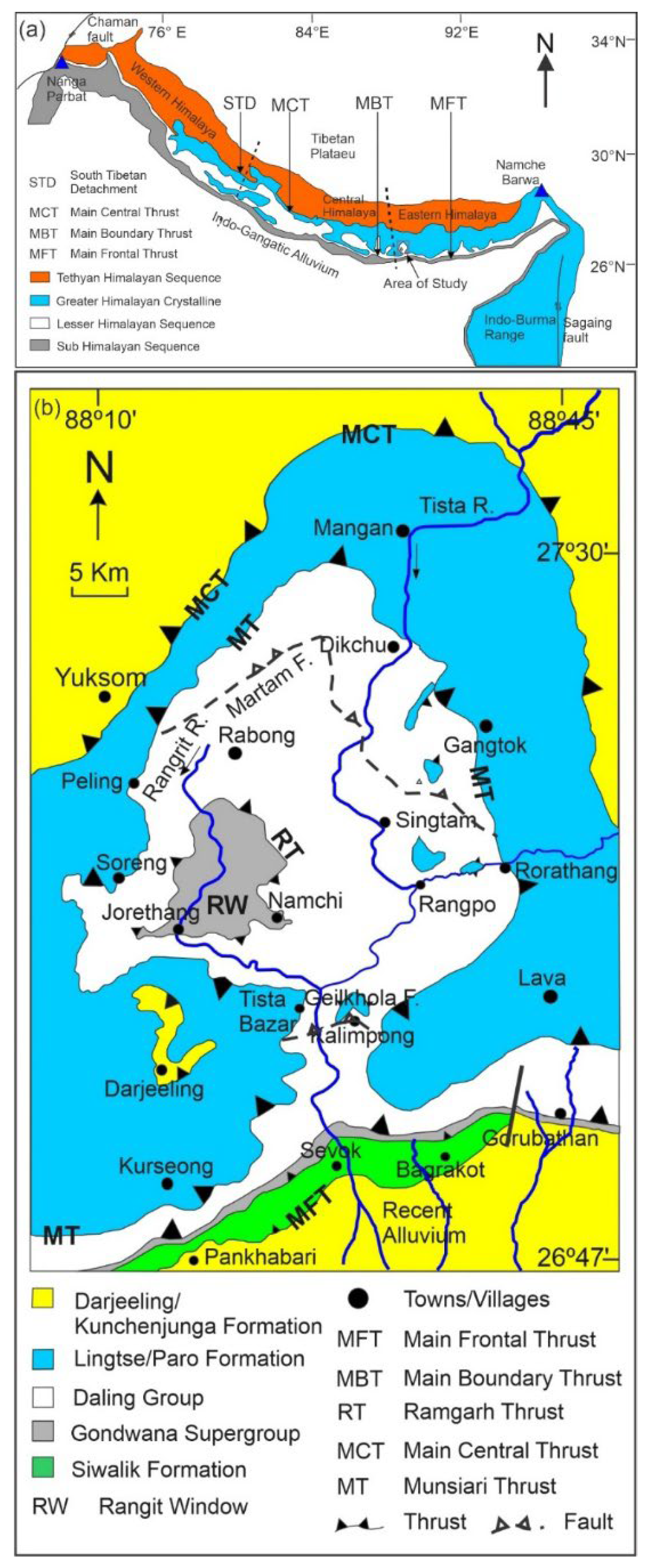
Figure 2.
Slope units and Landslide inventory overlaid on the Digital Elevation Model (DEM), showing the spatial relationship between terrain morphology and landslide occurrence.
Figure 2.
Slope units and Landslide inventory overlaid on the Digital Elevation Model (DEM), showing the spatial relationship between terrain morphology and landslide occurrence.
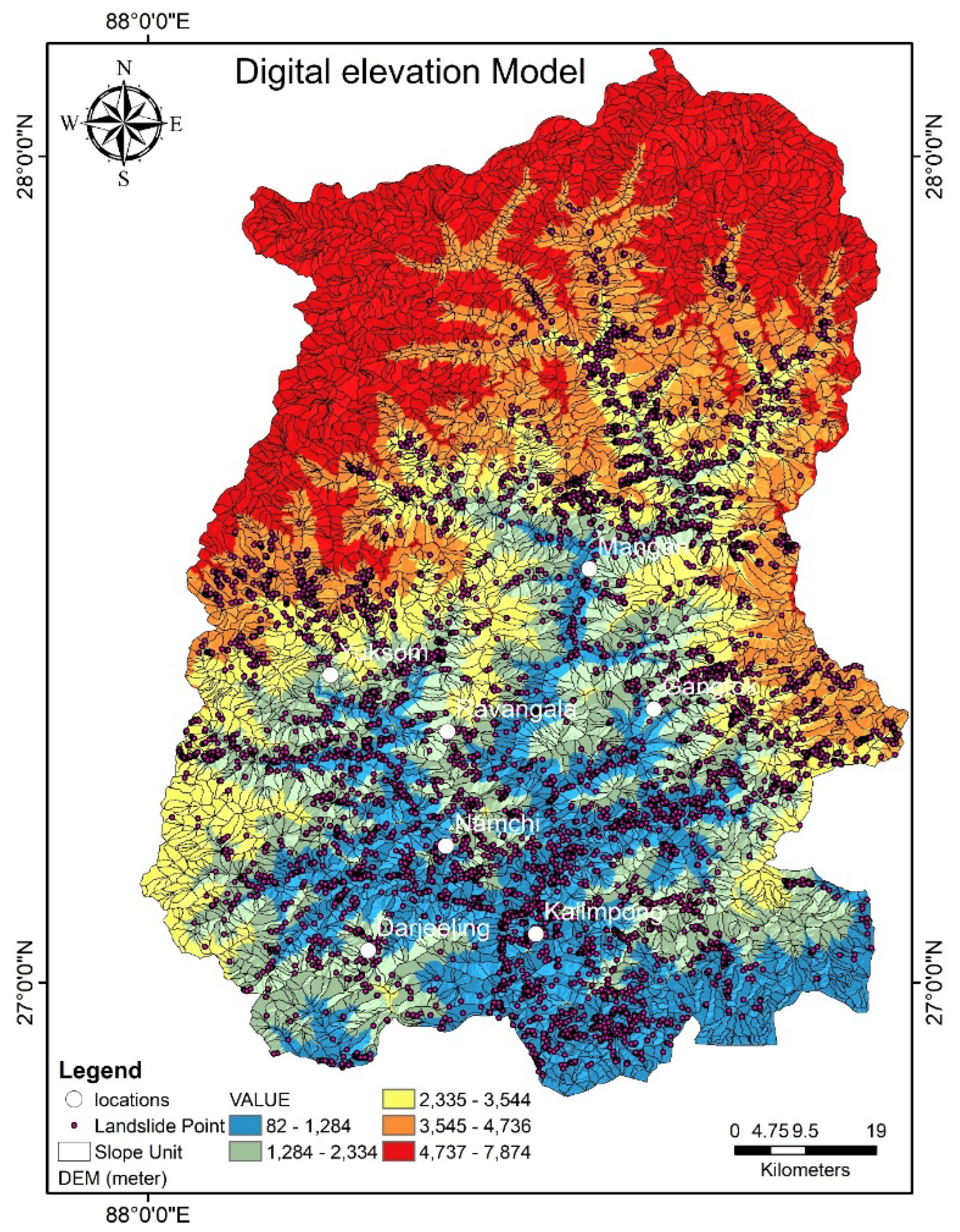
Figure 3.
Representation of the selected landslide conditioning factors and their classification used for modelling: (a) Elevation (DEM); (b) Aspect; (c) Slope; (d) Earthquake Intensity; (e) Normalized Difference Vegetation Index (NDVI); (f) Rainfall; (g) Lithology; (h) Distance to Streams; (i) Distance to Roads; (j) Distance to Lineaments; (k) Distance to Faults; (l) Soil Moisture; (m) Profile Curvature; (n) Plan Curvature; (o) Terrain Ruggedness Index (TRI); (p) Topographic Position Index (TPI); and (q) Topographic Wetness Index (TWI).
Figure 3.
Representation of the selected landslide conditioning factors and their classification used for modelling: (a) Elevation (DEM); (b) Aspect; (c) Slope; (d) Earthquake Intensity; (e) Normalized Difference Vegetation Index (NDVI); (f) Rainfall; (g) Lithology; (h) Distance to Streams; (i) Distance to Roads; (j) Distance to Lineaments; (k) Distance to Faults; (l) Soil Moisture; (m) Profile Curvature; (n) Plan Curvature; (o) Terrain Ruggedness Index (TRI); (p) Topographic Position Index (TPI); and (q) Topographic Wetness Index (TWI).
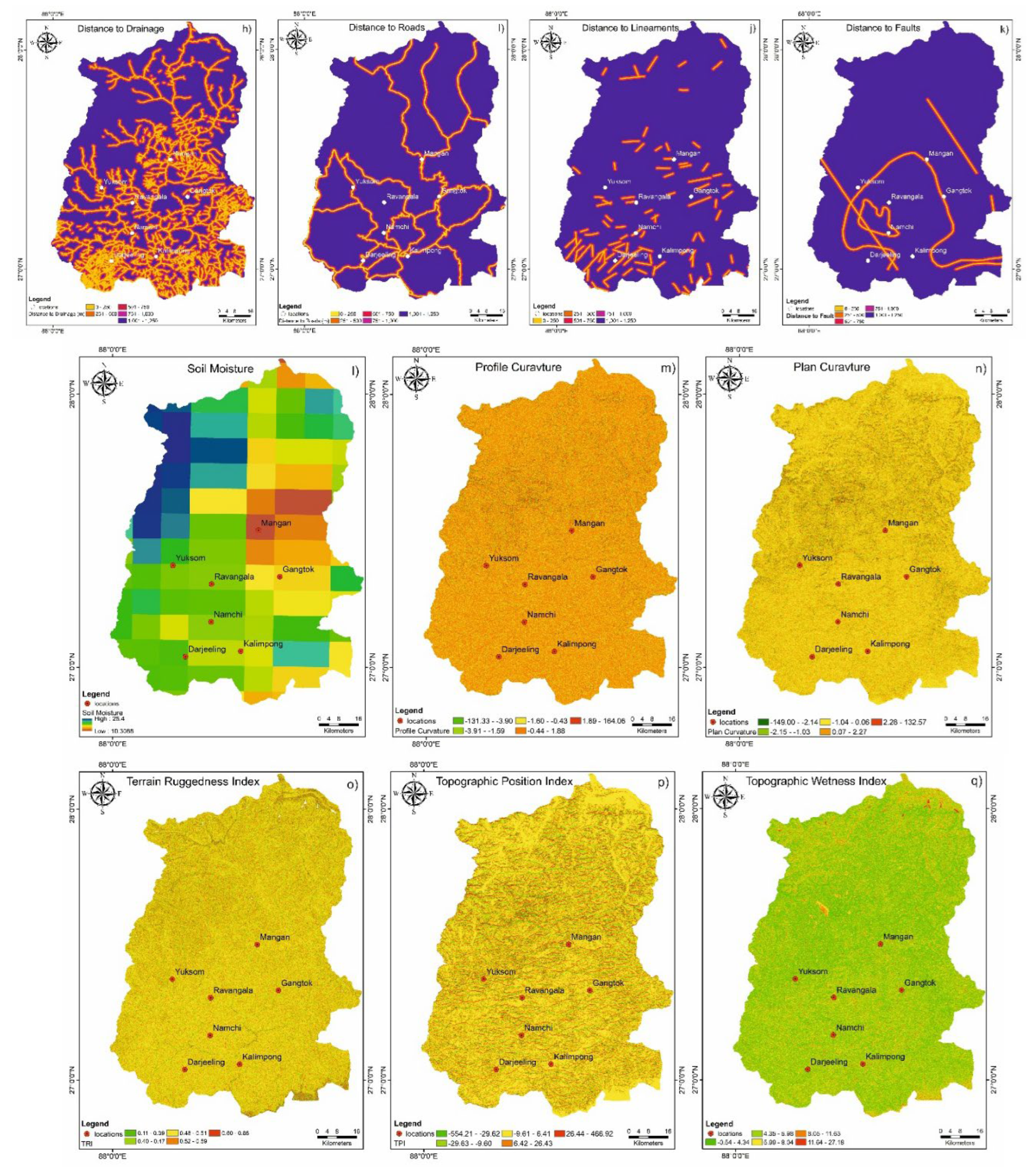
Figure 4.
The methodological workflow for slope-unit-based Landslide Susceptibility Mapping.
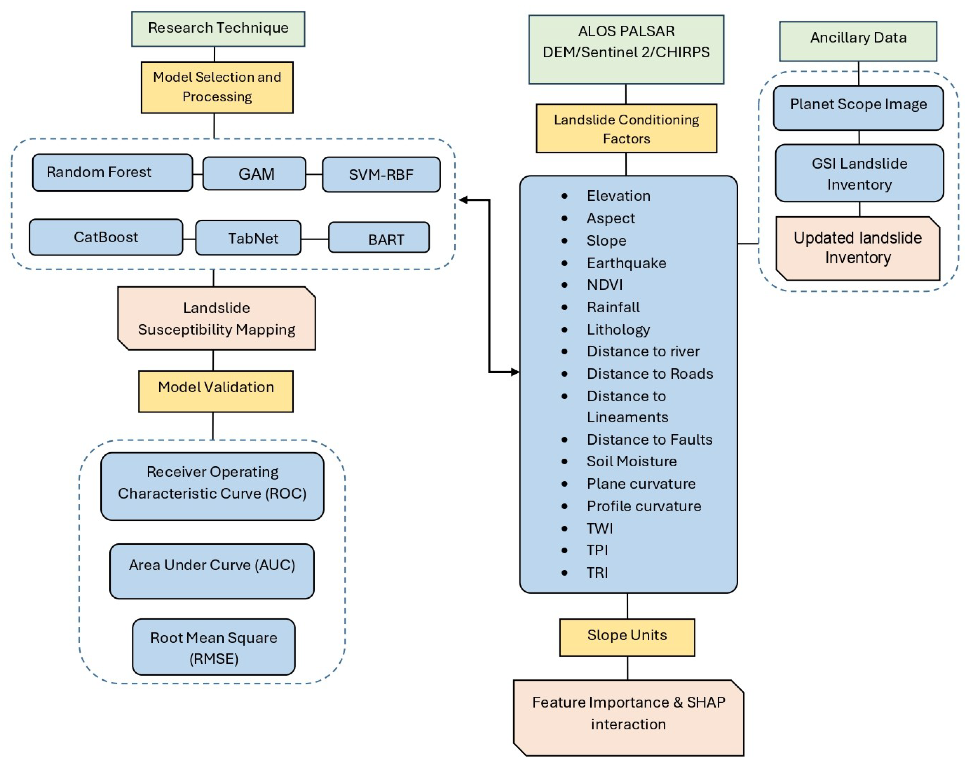
Figure 5.
SHAP summary plots and corresponding feature importance charts for (a) Random Forest (RF) and (b) CatBoost models used in landslide susceptibility mapping.
Figure 5.
SHAP summary plots and corresponding feature importance charts for (a) Random Forest (RF) and (b) CatBoost models used in landslide susceptibility mapping.
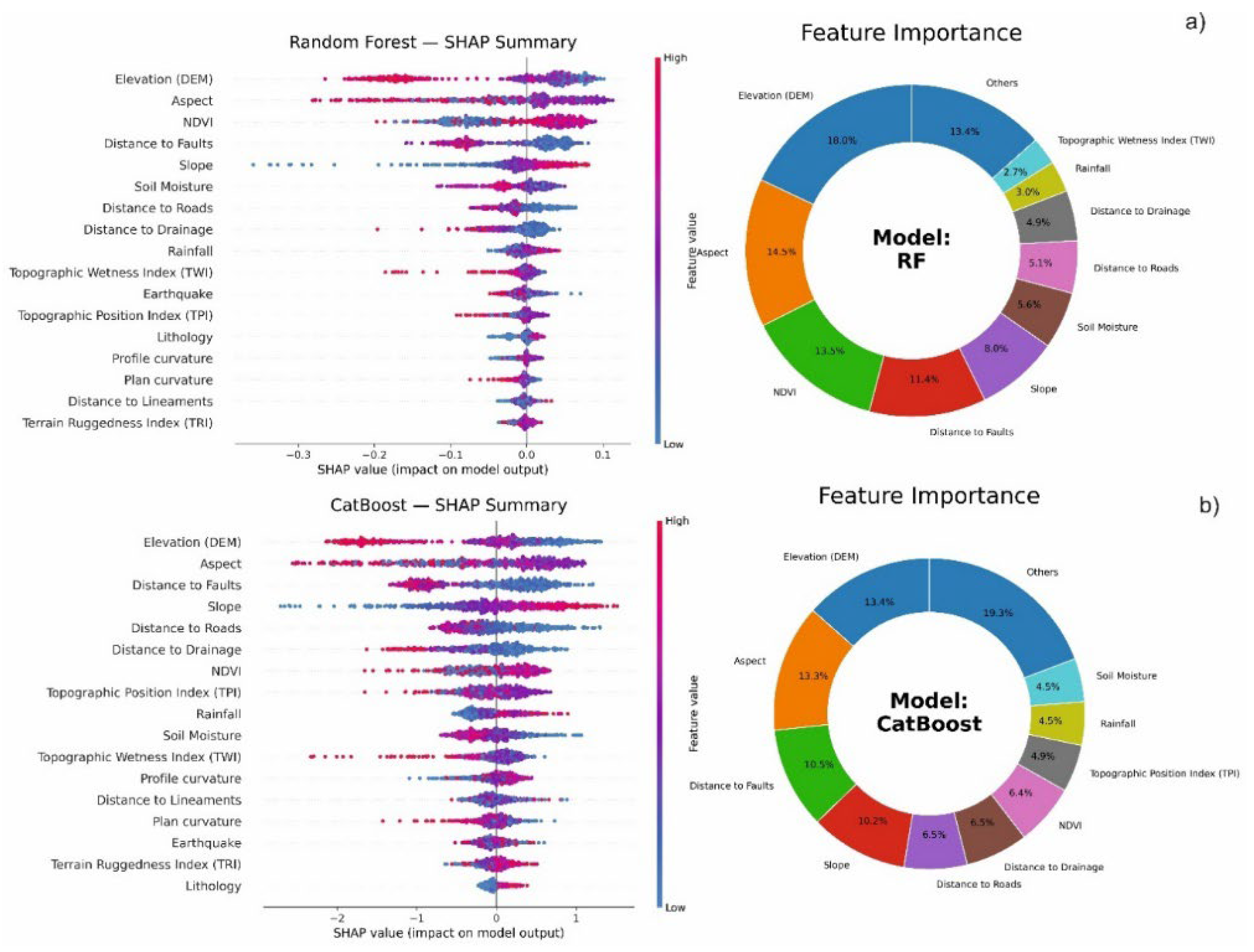
Figure 6.
SHAP-based interaction analysis illustrating the combined influence of key conditioning factors on landslide susceptibility. The dependence plots show the relationship between feature values (x-axis) and their SHAP contributions (y-axis), with color representing the interacting variable. (a) Slope × Rainfall, (b) Slope × Distance to Roads, (c) Slope × Distance to Drainage, (d) Rainfall × Soil Moisture, and (e) Slope × Distance to Faults.
Figure 6.
SHAP-based interaction analysis illustrating the combined influence of key conditioning factors on landslide susceptibility. The dependence plots show the relationship between feature values (x-axis) and their SHAP contributions (y-axis), with color representing the interacting variable. (a) Slope × Rainfall, (b) Slope × Distance to Roads, (c) Slope × Distance to Drainage, (d) Rainfall × Soil Moisture, and (e) Slope × Distance to Faults.
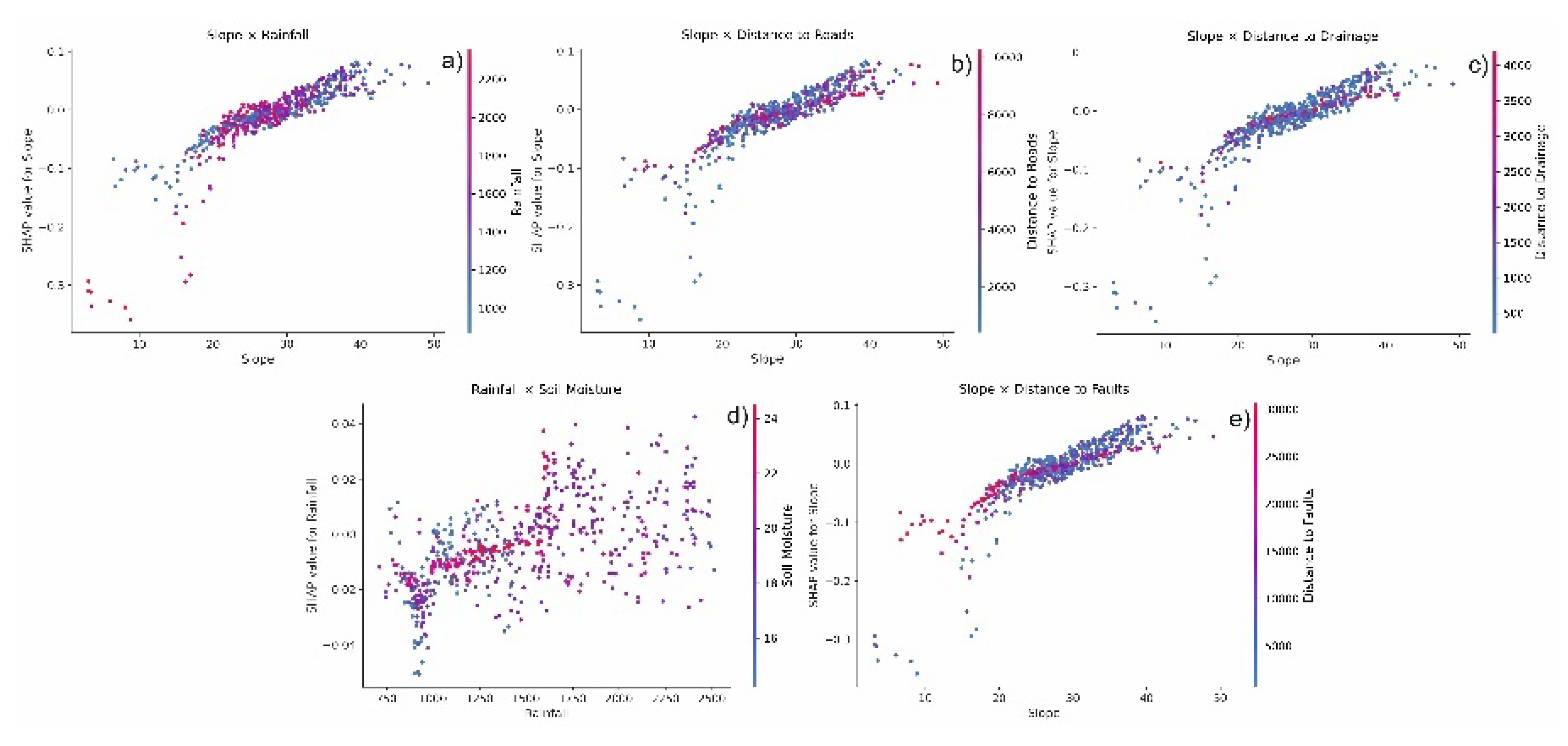
Figure 7.
Comparative Slope-unit-based landslide susceptibility maps produced using a. Random Forest (RF), b. Generalized Additive Model (GAM), c. CatBoost, d. TabNet, e. BART, and f. CNN are presented for visual comparison.
Figure 7.
Comparative Slope-unit-based landslide susceptibility maps produced using a. Random Forest (RF), b. Generalized Additive Model (GAM), c. CatBoost, d. TabNet, e. BART, and f. CNN are presented for visual comparison.
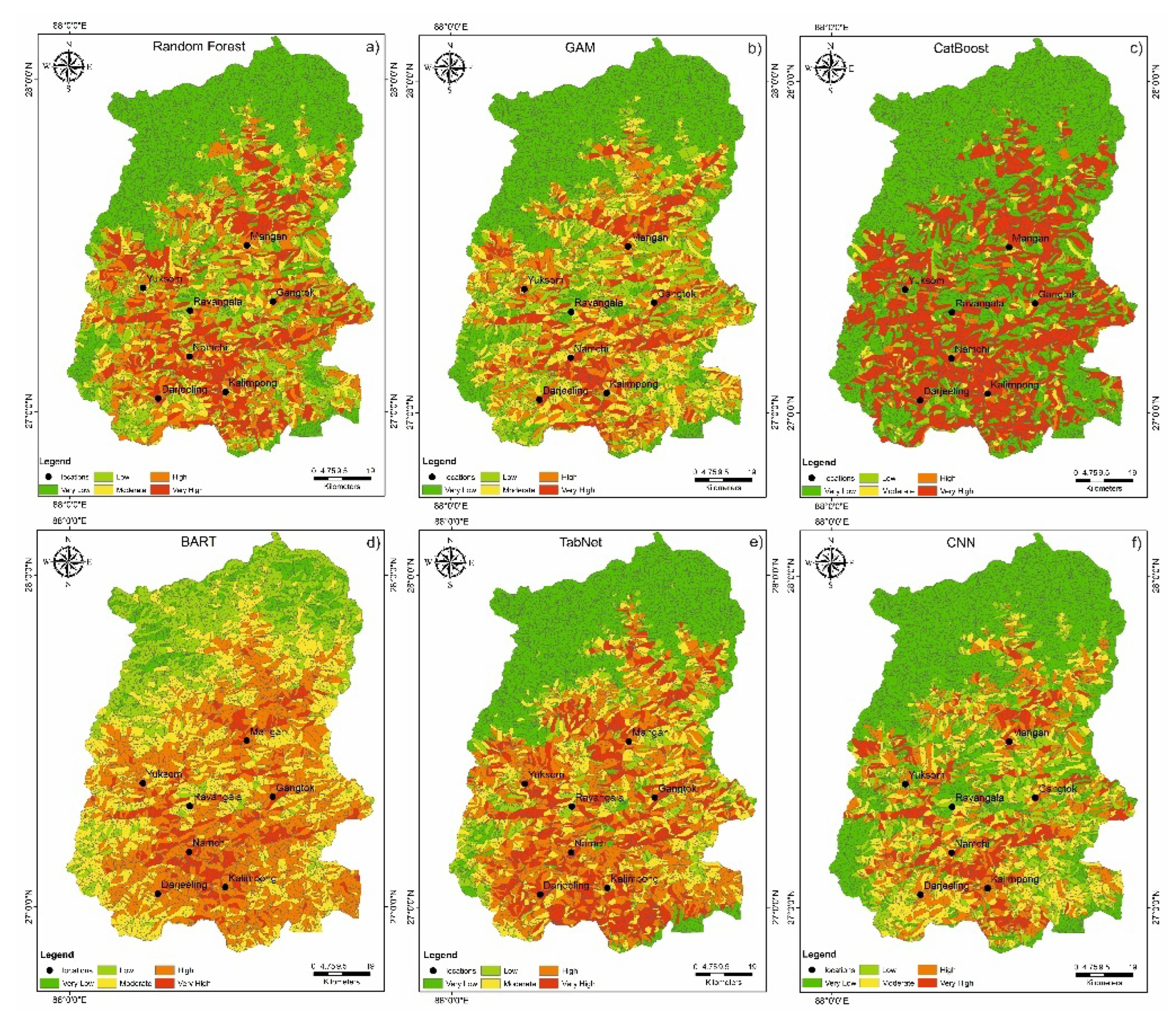
Figure 8.
Distribution of slope units, landslide occurrence, and area percentage across landslide susceptibility classes derived using model-specific natural breaks using six machine-learning models: (a) Random Forest (RF), (b) Generalized Additive Model (GAM), (c) CatBoost, (d) TabNet, (e) Bayesian Additive Regression Trees (BART), and (f) Convolutional Neural Network (CNN).
Figure 8.
Distribution of slope units, landslide occurrence, and area percentage across landslide susceptibility classes derived using model-specific natural breaks using six machine-learning models: (a) Random Forest (RF), (b) Generalized Additive Model (GAM), (c) CatBoost, (d) TabNet, (e) Bayesian Additive Regression Trees (BART), and (f) Convolutional Neural Network (CNN).
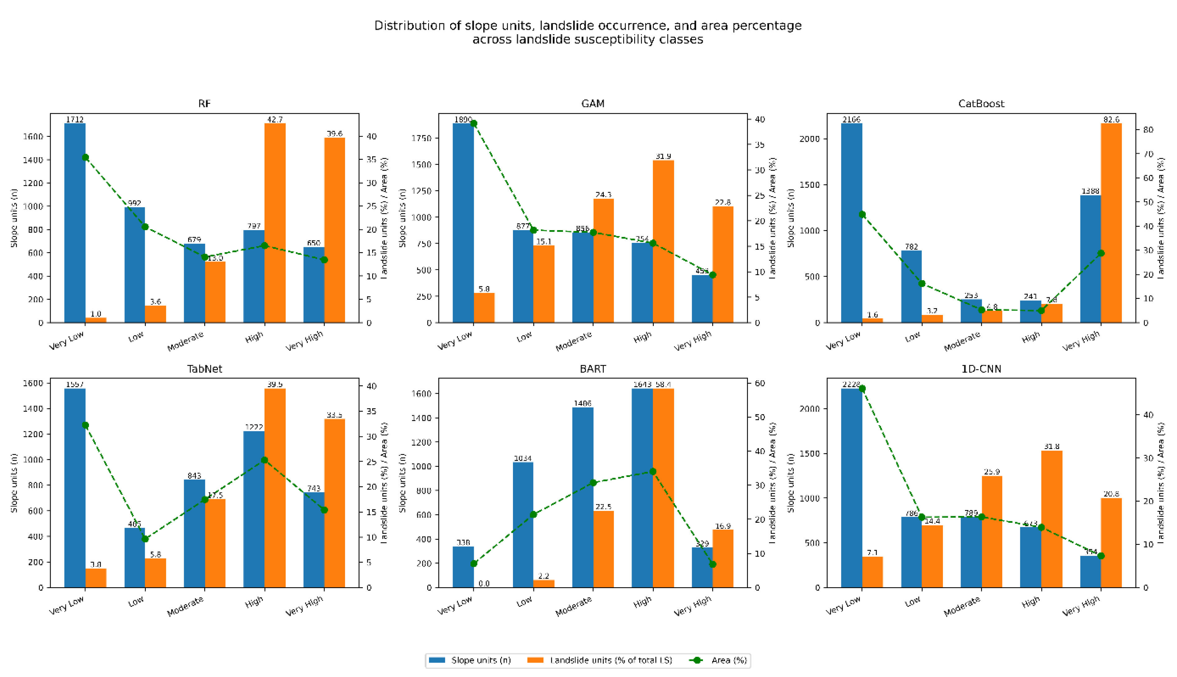
Figure 9.
Receiver Operating Characteristic (ROC) curves of all landslide susceptibility models. ROC curves for RF, GAM, CatBoost, TabNet, BART, and CNN, and Area Under the Curve (AUC) values quantify the discriminative ability of each model.
Figure 9.
Receiver Operating Characteristic (ROC) curves of all landslide susceptibility models. ROC curves for RF, GAM, CatBoost, TabNet, BART, and CNN, and Area Under the Curve (AUC) values quantify the discriminative ability of each model.
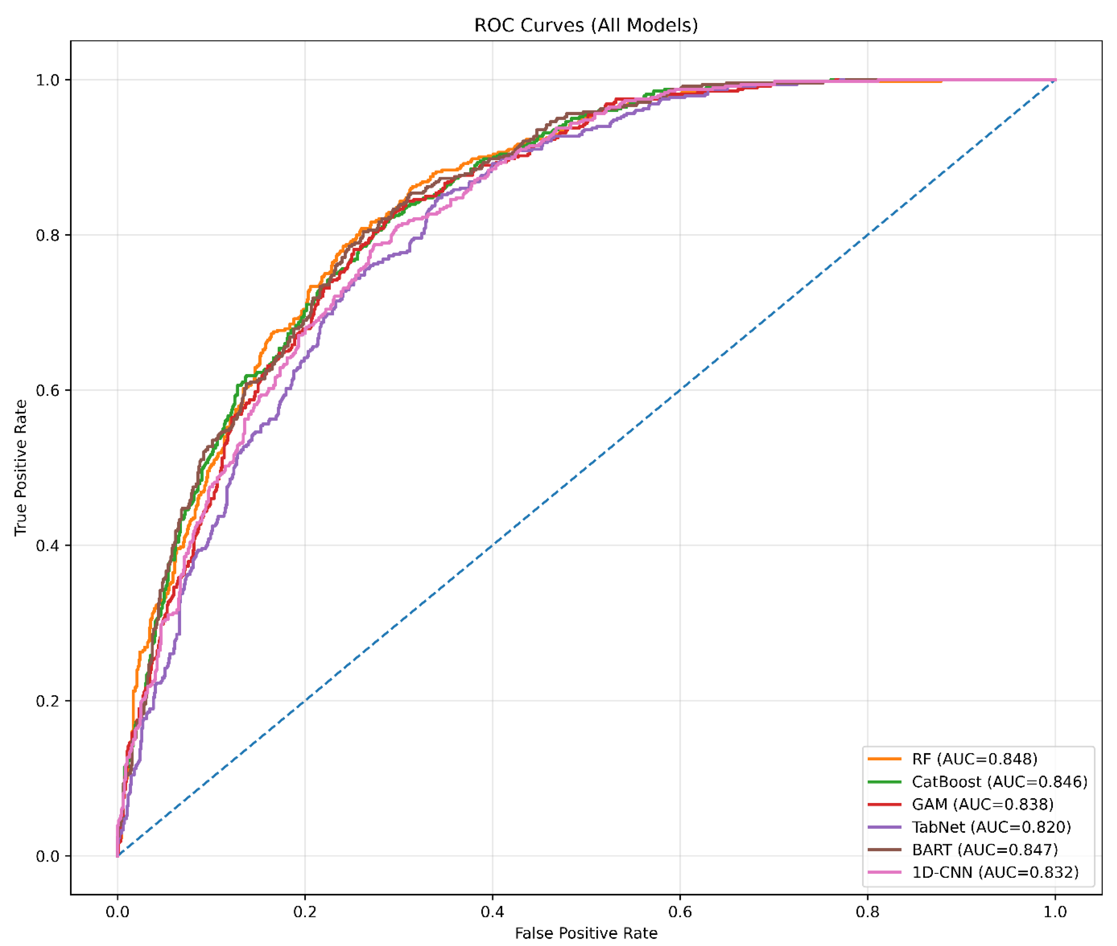
Table 1.
Summary of the complete landslide inventory used in the study.
| Attribute | Description |
|---|---|
| Inventory type | Multi-temporal landslide inventory |
| Total number of landslides | 8373 |
| Landslide representation | Point |
| Mapping method | GSI inventory, Manual Mapping, field validation |
| Temporal coverage | 1974 to 2024 |
| Total Number of Slope Units | 4830 |
| Slope units with non-landslides | 3231 |
| Slope units with landslides | 1599 |
Table 2.
Conditioning factors selected for slope-unit-based landslide susceptibility modelling and their data sources.
Table 2.
Conditioning factors selected for slope-unit-based landslide susceptibility modelling and their data sources.
| S.No | Conditioning Factors | Data Source | Spatial Resolution |
|---|---|---|---|
| 1. | Elevation (DEM) | ALOS PALSAR DEM | 12.5 m |
| 2. | Slope | ALOS PALSAR DEM | 12.5 m |
| 3. | Aspect | ALOS PALSAR DEM | 12.5 m |
| 4. | NDVI | Sentinel 2 | 10 m |
| 5. | Rainfall | CHIRPS | 5 km (resampled to 12.5 m) |
| 6. | Earthquake | USGS Earthquake Catalog and National Centre for Seismology | Point-based data |
| 7. | Soil Moisture | SMAP (Soil Moisture Active Passive, NASA) | ~9 km (resampled to 12.5 m) |
| 8. | Distance to Drainage | Open Street Map | Vector data |
| 9. | Distance to Faults | Geological Survey of India | Vector data |
| 10. | Distance to Lineaments | Geological Survey of India | Vector data |
| 11. | Distance to Roads | Open Street Map | Vector data |
| 12. | Lithology | Geological Survey of India | 1:50,000 |
| 13. | Topographic Wetness Index (TWI) | ALOS PALSAR DEM | 12.5 m |
| 14. | Terrain Ruggedness Index (TRI) | ALOS PALSAR DEM | 12.5 m |
| 15. | Topographic Position Index (TPI) | ALOS PALSAR DEM | 12.5 m |
| 16. | Profile curvature | ALOS PALSAR DEM | 12.5 m |
| 17. | Plan curvature | ALOS PALSAR DEM | 12.5 m |
Table 3.
Bayesian Optimization based hyperparameters used in all six models for Landslide Susceptibility Mapping.
Table 3.
Bayesian Optimization based hyperparameters used in all six models for Landslide Susceptibility Mapping.
| Model | Hyperparameter | Optimal value |
|---|---|---|
| Random Forest | n_estimators Max depth Min Samples leaf Min samples split Max features Bootstrap |
1262 33 4 2 Log2 True |
| GAM | Model Type Smooth terms Decision threshold Link function Imputation Smoothing parameter (Y) |
Logistic GAM s(0)-s(16) 0.32 logit median 0.4 |
| CatBoost | Number of iterations Learning rate Tree depth L2 regularization Loss function Class weights Random Strength Bagging temperature Border count |
1703 0.039 8 20.92 Logloss Balanced 0.93 0.80 179 |
| TabNet | n_d n_a n_steps Lambda_sparse Optimiser Learning_rate Batch_size Gamma mask_type virtual_batch_size |
40 48 7 0.0006 Adam 0.02 512 1.74 Sparsemax 256 |
| BART | n_trees n_burn n_samples n_chains |
200 200 800 4 |
| CNN | Conv1 filters Conv2 filters Kernel size Dense units Dropout Learning rate Batch size Weight decay |
32 96 3 64 0.599 0.00136 128 3.22x10⁻⁵ |
Disclaimer/Publisher’s Note: The statements, opinions and data contained in all publications are solely those of the individual author(s) and contributor(s) and not of MDPI and/or the editor(s). MDPI and/or the editor(s) disclaim responsibility for any injury to people or property resulting from any ideas, methods, instructions or products referred to in the content. |
© 2026 by the authors. Licensee MDPI, Basel, Switzerland. This article is an open access article distributed under the terms and conditions of the Creative Commons Attribution (CC BY) license (http://creativecommons.org/licenses/by/4.0/).
Copyright: This open access article is published under a Creative Commons CC BY 4.0 license, which permit the free download, distribution, and reuse, provided that the author and preprint are cited in any reuse.